title regeneration cycle and the covariant lyapunov
TRANSCRIPT
RIGHT:
URL:
CITATION:
AUTHOR(S):
ISSUE DATE:
TITLE:
Regeneration cycle and thecovariant Lyapunov vectors in aminimal wall turbulence.
Inubushi, Masanobu; Takehiro, Shin-Ichi; Yamada,Michio
Inubushi, Masanobu ...[et al]. Regeneration cycle and the covariant Lyapunov vectors in aminimal wall turbulence.. Physical review E 2015, 92(2): 023022.
2015-08-24
http://hdl.handle.net/2433/201954
©2015 American Physical Society
PHYSICAL REVIEW E 92, 023022 (2015)
Regeneration cycle and the covariant Lyapunov vectors in a minimal wall turbulence
Masanobu Inubushi,* Shin-ichi Takehiro,† and Michio Yamada‡
Research Institute for Mathematical Sciences, Kyoto University, Kyoto, Japan(Received 21 January 2013; revised manuscript received 9 June 2015; published 24 August 2015)
Considering a wall turbulence as a chaotic dynamical system, we study regeneration cycles in a minimal wallturbulence from the viewpoint of orbital instability by employing the covariant Lyapunov analysis developedby F. Ginelli et al. [Phys. Rev. Lett. 99, 130601 (2007)]. We divide the regeneration cycle into two phases andcharacterize them with the local Lyapunov exponents and the covariant Lyapunov vectors of the Navier-Stokesturbulence. In particular, we show numerically that phase (i) is dominated by instabilities related to the sinuousmode and the streamwise vorticity, and there is no instability in phase (ii). Furthermore, we discuss a mechanismof the regeneration cycle, making use of an energy budget analysis.
DOI: 10.1103/PhysRevE.92.023022 PACS number(s): 47.52.+j, 05.45.−a, 47.27.N−
I. INTRODUCTION
Toward an understanding of wall turbulence based on theNavier-Stokes equations, we characterize a wall turbulencein terms of orbital instability of chaos. The orbital instabilityis quantified by Lyapunov exponents and Lyapunov vectors.While the Lyapunov exponent λ is an exponential growth rateof the norm of the perturbation vector added to a chaotic orbit,the Lyapunov vector y is the perturbation vector whose normgrows exponentially as || y(t)|| ∝ eλt . The Lyapunov expo-nents and vectors characterize stabilities of a chaotic attractor,just as eigenvalues and eigenvectors characterize stabilitiesof a fixed point attractor. Ginelli et al. [1] developed thecovariant Lyapunov analysis, proposing a numerical algorithmto calculate both Lyapunov exponents and vectors. Whilethe covariant Lyapunov analysis has been applied to variousdynamical systems to study their chaotic properties suchas hyperbolicity, effective dimension, and inertial manifold[2–7] (see review papers [8–10] and references therein), ithas not been applied to the three-dimensional Navier-Stokesequations. In this paper, by using this algorithm, we studythe orbital instability of the regeneration cycle in the wallturbulence governed by the Navier-Stokes equations.
Wall turbulence has been studied as a typical turbulenceassociated with the wall boundary. To find out a “minimal”mechanism producing wall turbulence, Jimenez and Moin [11]and Hamilton et al. [12] searched numerically the minimalsize of the periodic box (minimal flow unit) in which we canobserve turbulence. As a result, in the minimal flow units,they found regeneration cycles consisting of breakdown andreformation of the coherent structures such as streamwisevortices and streaks which are high or low streamwise velocityregions in Poiseuille turbulence [11] and in Couette turbulence[12]. The regeneration cycle has been observed in many typesof wall turbulence (Panton [13]) and was recently observed inexperiments of boundary layer turbulence by Duriez et al. [14].
In order to describe the regeneration cycle, Hamilton et al.[12] and Waleffe [15] proposed a mechanism (which they call
*[email protected]; Present address: NTT Commu-nication Science Laboratories, NTT Corporation.†[email protected]‡[email protected]
self-sustaining process) which consists of streak instability,regeneration of the streamwise vortices, and reformation ofthe streaks, by modeling the streaks and the streamwisevortices. On the streak instability, Schoppa and Hussain [16]investigated linear stability of model streaks numerically andfound that these models are linearly unstable to the sinuousinstability mode (see Fig. 9 in [16]) which causes meanderingof the straight streak as observed by Hamilton et al. [12]. Linearstability of a corrugated vortex sheet, which is an inviscidmodel of the streak, was studied by Kawahara et al. [17].They found the vortex sheet is linearly unstable to the sinuousdisturbance in a long-wave limit. There are numerous studieson linear stability of model streaks including the above models(see [17] and references therein) and most of them suggest thatthe sinuous mode is the most unstable perturbation.
Following the meanderings of the straight streaks, the flowchanges into fully three-dimensional turbulence, and stream-wise vortices are expected to be generated. To understandthis process, many mechanisms have been proposed such asWaleffe [15] and Jimenez and Moin [11] (see [18]). Once thestreamwise vortices are generated, these vortices advect thegradient of the streamwise velocity in the cross-streamwiseplane, which forms the streak structures. Kawahara [18]showed that an analytical model of the streamwise vortexforms the streak structures by the above mechanism. Waleffe[15] derived a low-dimensional ODE model for understandingof the regeneration cycle. While these models and their resultsare suggestive, the mechanisms of the regeneration cycleshould be clarified based on the full Navier-Stokes equations.
One of the crucial steps toward understanding of theregeneration cycle on the basis of the full Navier-Stokesequation is finding of the unstable periodic orbit (UPO)by Kawahara and Kida [19] which approximates turbulentstatistics very well. Recently, a lot of invariant solutionsof the full Navier-Stokes equation and the (homoclinic andheteroclinic) connections between them have been foundnumerically and used to clarify the state space structures forunderstanding mechanisms of the regeneration cycle [20–24](see Kawahara [25] for the detailed review).
The main questions we study here are as follows: Can weclarify the mechanisms underlying the regeneration cycle with-out using the ad hoc models? How does the orbital instabilitiesplay roles in the regeneration cycle? To answer these questions,we characterize the regeneration cycle in the minimal Couette
1539-3755/2015/92(2)/023022(14) 023022-1 ©2015 American Physical Society
A Self-archived copy inKyoto University Research Information Repository
https://repository.kulib.kyoto-u.ac.jp
INUBUSHI, TAKEHIRO, AND YAMADA PHYSICAL REVIEW E 92, 023022 (2015)
turbulence with the covariant Lyapunov analysis applied tothe full Navier-Stokes equation. We formulate the problemin Sec. II, and describe the covariant Lyapunov analysis andthe numerical method in Sec. III. We show the turbulentbehaviors of the minimal Couette turbulence, particular theregeneration cycle in Sec. IV. In Sec. V, we show the mainresult of this paper: the orbital instability of the regenerationcycle in the minimal Couette turbulence. In order to discuss thestreak reformation, we study the energy budget of the minimalCouette turbulence in Sec. VI. Finally, we give our conclusionand discussion in Sec. VII.
II. MINIMAL COUETTE FLOW SYSTEM
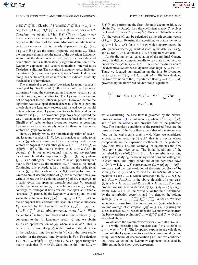
Plane Couette flow is a fluid system where incompressibleviscous fluid is in between upper and lower walls and the fluidmotion is driven by the walls moving in the opposite directionas shown in Fig. 1. We set the streamwise flux and the spanwisemean pressure gradient to be zero.
The nondimensionalized Navier-Stokes equation and theincompressible condition is
∂u∂t
+ (u · ∇)u = −∇p + 1
Re∇2u,
(1)∇ · u = 0,
where u = (ux,uy,uz) is the velocity, and p is the pressuredefined in the domain (x,y,z) ∈ [0,Lx] × [0,Ly] × [−1,1].We use the nonslip boundary condition on the walls (z = ±1):
ux(x,y, ± 1) = ±1, (2)
uz(x,y, ± 1) = uy(x,y, ± 1) = 0, (3)
and the periodic boundary condition in a horizontal direction:
u(x,y,z) = u(x + Lx,y,z) = u(x,y + Ly,z), (4)
∇p(x,y,z) = ∇p(x + Lx,y,z) = ∇p(x,y + Ly,z). (5)
The Reynolds number is set to be Re = 400 and the domainsize is the minimal flow unit size: Lx = 1.755π,Ly = 1.2π .Decomposing the flow field into the toroidal and poloidalpotentials, we compute the time evolution of the potentials.
FIG. 1. Illustration of the plane Couette flow system. x, y, z
directions are referred to as streamwise, spanwise, wall-normaldirections, respectively.
The de-aliased Fourier expansions (2/3 rule) are employed inthe horizontal (x-y) directions, and the Chebyshev tau methodsare employed in the wall-normal (z) direction: ψ(x,y,z) =∑KM
k=−KM
∑LMl=−LM
∑MMm=0 ψ(k,l,m)e
i(αkx+βly)Tm(z), whereψ(k,l,m) is the expansion coefficient, α = 2π/Lx andβ = 2π/Ly are the fundamental streamwise and spanwisewave numbers, respectively, and Tm(z) is the mth-orderChebyshev polynomial. We set the truncation mode numbersKM = 8 (x direction), LM = 8 (y direction), MM = 32 (zdirection), and the computational grid points are 32 × 32 × 33(x,y,z directions). The dimension of the dynamical systemN is N = 2[(2KM + 1)(2LM + 1) − 1](MM + 1) +2(MM + 1) = 19 074. The time integration is performedwith the second-order Adams-Bashforth method with atime step width �t = 1.0 × 10⁻³. The CFL number is lessthan 0.1 which is less than Philip and Manneville [26]use in the similar setting. The friction Reynolds numberReτ (= uτh/ν) is Reτ = 34.0 and the periods of the domainin the streamwise and spanwise directions normalized bylτ = ν/uτ are L+
x = Lx/lτ = 187 and L+y = Ly/lτ = 128,
respectively, which is in good agreement with the valuesreported in Kawahara [19]. The grid spacing in the x,y, andz directions normalized by lτ is �x+ = 5.9, �y+ = 4.0,and �z+ = 0.16–3.3 (the minimum-maximum grid spacing),which is comparable to those in most direct numericalsimulations [12]. We used the library for spectral transformISPACK [27], its Fortran90 wrapper library the SPMODELlibrary [28], and the subroutine of LAPACK. For drawing thefigures, the products of the Dennou Ruby project [29] andgnuplot were used.
III. COVARIANT LYAPUNOV ANALYSIS
In this section we describe in some detail the computationalmethod for covariant Lyapunov analysis proposed by Ginelliet al. (2007) [1], and for its application to the present Navier-Stokes wall turbulence.
Let us consider a discrete dynamical system f : RN →RN , and we write time evolution of a state point xn ∈ RN
as xn+1 = f (xn). Infinitesimal perturbation vectors y(j )n (j =
1,2, . . . ,N ) added to a state point xn on the orbit evolve asy(j )n+1 = D f n y(j )
n where D f n is a N × N Jacobian matrix atxn. Then, the j th Lyapunov exponent λj (λ1 � λ2 � · · · �λN ) and its corresponding covariant Lyapunov vector y(j )
0 at astate point x0 are defined as follows:
λj = limk→±∞
1
kln
∣∣∣∣D f k y(j )0
∣∣∣∣, (6)
where D f k = D f k−1 ◦ D f k−2 ◦ · · · ◦ D f 0. A set of Lya-punov exponents {λ1,λ2, · · · ,λN } is referred to as a Lyapunovspectrum.
The definition of the Lyapunov exponents and the covariantLyapunov vectors (6) does not depend on the choice of thenorm. The state space is finite dimensional and thus allnorms are equivalent; i.e., for arbitrary norms || · ||A,|| · ||B ,there exist positive real numbers αi (i = 1,2) such thatα1||x||A � ||x||B � α2||x||A for all x ∈ RN . If we consider||D f k y(j )
0 ||A and ||D f k y(j )0 ||B in the definition (6), there
exist α1 and α2 such that α1||D f k y(j )0 ||A � ||D f k y(j )
0 ||B �
023022-2
A Self-archived copy inKyoto University Research Information Repository
https://repository.kulib.kyoto-u.ac.jp
REGENERATION CYCLE AND THE COVARIANT LYAPUNOV . . . PHYSICAL REVIEW E 92, 023022 (2015)
α2||D f k y(j )0 ||A. Clearly, if 1/k ln(||D f k y(j )
0 ||A) → λj (k →∞), then 1/k ln(αi ||D f k y(j )
0 ||A) → λj (k → ∞) for i = 1,2.Therefore, we obtain 1/k ln(||D f k y(j )
0 ||B) → λj (k → ∞)from the above inequality, implying the definition (6) does notdepend on the choice of the norm. Moreover, an infinitesimalperturbation vector that is linearly dependent on y(j )
0 (i.e.,a y(j )
0 ,a ∈ R) gives the same Lyapunov exponent λj . Thus,the important thing is not the norm of the covariant Lyapunovvector, but the direction of it. See [8–10] for more detaileddescriptions and a mathematically rigorous definition of theLyapunov exponents and vectors (sometimes referred to asOseledets’ splitting). The covariant Lyapunov vector indicatesthe intrinsic (i.e., norm-independent) stable/unstable directionalong the chaotic orbit, which is expected to indicate instabilitymechanisms of turbulence.
The numerical algorithm of covariant Lyapunov analysisdeveloped by Ginelli et al. (2007) gives both the Lyapunovexponents λj and the corresponding Lyapunov vectors y(j )
n ata state point xn on the attractor. The Lyapunov vectors arenot orthogonal to each other in general. However, before thealgorithm was developed, there had been no efficient algorithmto calculate the Lyapunov vectors, and instead we just couldobtain orthogonalized Lyapunov vectors which depend on thenorm we use [30]. The covariant Lyapunov analysis paved theway to calculate the Lyapunov vectors as defined above. WhileGinelli et al. refer to these Lyapunov vectors as covariantLyapunov vectors, we simply refer to them as Lyapunovvectors or Lyapunov modes.
Here, we briefly review the numerical algorithm of covari-ant Lyapunov analysis [1,9]. Let us consider an orthogonalmatrix Q0 whose column vectors are arbitrary perturbationvectors orthogonal to each other qi
0 (i = 1,2, . . . ,N ) as Q0 =(q1
0|q20| · · · |qN
0 ). The matrix evolves as Qi+1 = D f iQi . Ingeneral, Qi is not an orthogonal matrix, and we performthe Gram-Schmidt decomposition as Qi+1 = Qi+1Ri+1 whereQi+1 is an orthogonal matrix and Ri is an upper-triangularmatrix. For later use, the matrices Qi,Ri have to be stored.Continuing this procedure, i.e., transferring the orthogonalmatrix Qi by the Jacobian matrix D f i and performing theGram-Schmidt decomposition of Qi for sufficient times (wewrite n � 0), the first column vector q1
n of Qn converges toa basis vector that spans an unstable subspace V 1
n spannedby the Lyapunov vector y1
n, the column vectors q1n and q2
n
converge to orthogonal basis vectors that span an unstablesubspace V 2
n spanned by the Lyapunov vectors y1n and y2
n, andso on; the column vectors q1
n,q2n, . . . ,q
jn (j = 1,2, . . . ,N ) are
the orthogonal basis vectors that span an unstable subspaceV
jn spanned by the Lyapunov vectors y1
n, y2n, . . . ,yj
n. Letv
j
l ∈ Vj
l \V j−1l be an arbitrary vector, where l � n. When
the vector vj
l is transferred backward in time sufficiently, vj
l
converges to the j th Lyapunov vector yj
l , and we obtainv
jm as an approximation of yj
m where n � m � l. This isbecause a direction along yj
m is the most unstable directionin the backward time dynamics in V
jm (i.e., the most stable
direction in the forward time dynamics in Vjm). To calculate
vjm, let Ul = (v1
l |v2l | · · · |vN
l ) and Cl be an upper-triangularmatrix such that Ul = QlCl . Substituting this into Ul+1 =
D f lUl and performing the Gram-Schmidt decomposition, weobtain Cl+1 = Rl+1Cl ; i.e., the coefficient matrix Cl evolvesbackward in time as Cl−1 = R−1
l Cl . Once we obtain the matrixCm, the vector v
jm can be calculated as the j th column vector
of Um = QmCm. By using this algorithm, we obtain the vectorv
j
i (j = 1,2, . . . ,N ) for n < i < m which approximates thej th Lyapunov vector yj
i , while discarding the data such as Qi
and Ui for 0 � i � n and m � i � l as the transient data.As for the numerical calculation of the minimal Couette
flow, it is difficult computationally to calculate all of the Lya-punov vectors y(j )(t) (j = 1,2, . . . ,N ) since the dimension ofthe dynamical system we study here is too high (N = 19 074).Thus, we focused our attention on the first 30 Lyapunovvectors, i.e., y(j )(t) (j = 1,2, . . . ,M; M = 30). We calculatedthe time evolution of the j th perturbed flow (j = 1,2, . . . ,M)governed by the linearized Navier-Stokes equation:
∂uj
∂t+ (uj · ∇)u + (u · ∇)uj = −∇pj + 1
Re∇2uj ,
(7)∇ · uj = 0,
while calculating the base flow u governed by the Navier-Stokes equations (1) simultaneously, where uj = (uj
x,ujy,u
jz )
and pj are the velocity and pressure field of the perturbedflow. The boundary conditions of the perturbed flows are thesame as those of the base flow except that of the streamwiseflow on the walls: u
jx(x,y, ± 1) = 0. Here, we considered
a perturbation vector qj (t) ∈ RN that is a vector whosecomponents are the expansion coefficients of the perturbedflow field uj (t); i.e., the vector qj (t) determines the flowfield uj (t) and vice versa. The initial conditions of theperturbed flows uj (0) (j = 1,2, . . . ,M) are arbitrary as longas they are satisfying the boundary conditions and orthogonalto each other. The initial conditions of the perturbed flowsuj (0) (j = 1,2, . . . ,M) correspond to Q0 = (q1
0|q20| · · · |qM
0 ).We calculated the time evolution of the perturbed flow uj bysolving the Eq. (7), and performed the Gram-Schmidt decom-position at each T = 1, which correspond to Qi+1 = D f iQi
and Qi+1 = Qi+1Ri+1 in the above algorithm. In our case,Qi is a N × M matrix and Ri is a M × M matrix. The innerproduct we use here is defined by ( y1, y2)E = 1
2 〈ω1 · ω2〉Vwhere ωi(i = 1,2) is the vorticity vector field determinedby the perturbation vector yi and 〈·〉V denotes the volumeaverage: 〈·〉V = 1
2LxLy
∫ z=+1z=−1
∫ y=Ly
y=0
∫ x=Lx
x=0 ·dxdydz. We usedan induced norm from the inner product (·,·)E which is avolume average of enstrophy: || y||2 = ( y, y)E . By using thestored matrices Qi,Ri , we obtained the Lyapunov vectors fromthe backward time evolution Ci−1 = R−1
i Ci and Ui = QiCi asdescribed above.
We obtained the Lyapunov vectors for T = 23 000 (= m −n − 1) while discarding the transient data for T = 5000 (=n + 1 = m − l + 1). The Lyapunov exponents are calculatedfrom both the Lyapunov vectors and the conventional methodusing Gram-Schmidt decomposition [30], and we confirmedthat these values of the Lyapunov exponents calculated bydifferent methods show good agreement.
023022-3
A Self-archived copy inKyoto University Research Information Repository
https://repository.kulib.kyoto-u.ac.jp
INUBUSHI, TAKEHIRO, AND YAMADA PHYSICAL REVIEW E 92, 023022 (2015)
-0.04
-0.03
-0.02
-0.01
0
0.01
0.02
0.03
5 10 15 20 25 30
index
T=14 000T=17 000T=20 000T=23 000
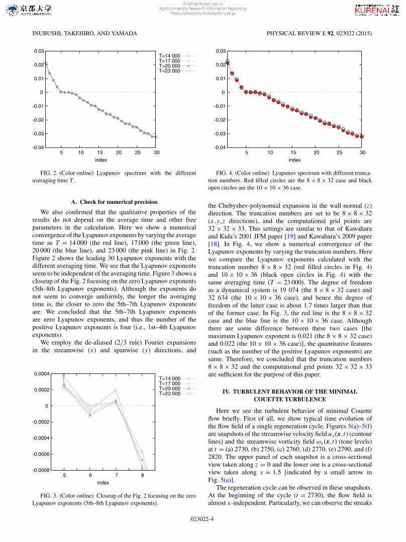
FIG. 2. (Color online) Lyapunov spectrum with the differentaveraging time T .
A. Check for numerical precision
We also confirmed that the qualitative properties of theresults do not depend on the average time and other freeparameters in the calculation. Here we show a numericalconvergence of the Lyapunov exponents by varying the averagetime as T = 14 000 (the red line), 17 000 (the green line),20 000 (the blue line), and 23 000 (the pink line) in Fig. 2.Figure 2 shows the leading 30 Lyapunov exponents with thedifferent averaging time. We see that the Lyapunov exponentsseem to be independent of the averaging time. Figure 3 shows acloseup of the Fig. 2 focusing on the zero Lyapunov exponents(5th–8th Lyapunov exponents). Although the exponents donot seem to converge uniformly, the longer the averagingtime is, the closer to zero the 5th–7th Lyapunov exponentsare. We concluded that the 5th–7th Lyapunov exponentsare zero Lyapunov exponents, and thus the number of thepositive Lyapunov exponents is four (i.e., 1st–4th Lyapunovexponents).
We employ the de-aliased (2/3 rule) Fourier expansionsin the streamwise (x) and spanwise (y) directions, and
-0.0008
-0.0006
-0.0004
-0.0002
0
0.0002
0.0004
5 6 7 8
index
T=14 000T=17 000T=20 000T=23 000
FIG. 3. (Color online) Closeup of the Fig. 2 focusing on the zeroLyapunov exponents (5th–8th Lyapunov exponents).
-0.04
-0.03
-0.02
-0.01
0
0.01
0.02
0.03
5 10 15 20 25 30
index
FIG. 4. (Color online) Lyapunov spectrum with different trunca-tion numbers. Red filled circles are the 8 × 8 × 32 case and blackopen circles are the 10 × 10 × 36 case.
the Chebyshev-polynomial expansion in the wall-normal (z)direction. The truncation numbers are set to be 8 × 8 × 32(x,y,z directions), and the computational grid points are32 × 32 × 33. This settings are similar to that of Kawaharaand Kida’s 2001 JFM paper [19] and Kawahara’s 2009 paper[18]. In Fig. 4, we show a numerical convergence of theLyapunov exponents by varying the truncation numbers. Herewe compare the Lyapunov exponents calculated with thetruncation number 8 × 8 × 32 (red filled circles in Fig. 4)and 10 × 10 × 36 (black open circles in Fig. 4) with thesame averaging time (T = 23 000). The degree of freedomas a dynamical system is 19 074 (the 8 × 8 × 32 case) and32 634 (the 10 × 10 × 36 case), and hence the degree offreedom of the latter case is about 1.7 times larger than thatof the former case. In Fig. 3, the red line is the 8 × 8 × 32case and the blue line is the 10 × 10 × 36 case. Althoughthere are some difference between these two cases [themaximum Lyapunov exponent is 0.021 (the 8 × 8 × 32 case)and 0.022 (the 10 × 10 × 36 case)], the quantitative features(such as the number of the positive Lyapunov exponents) aresame. Therefore, we concluded that the truncation numbers8 × 8 × 32 and the computational grid points 32 × 32 × 33are sufficient for the purpose of this paper.
IV. TURBULENT BEHAVIOR OF THE MINIMALCOUETTE TURBULENCE
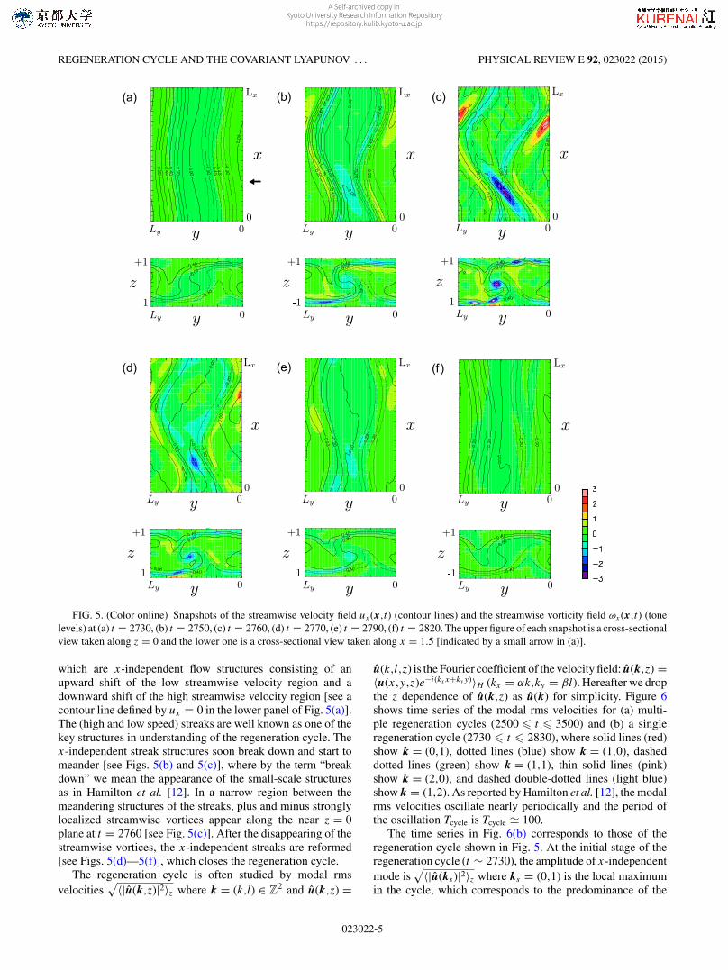
Here we see the turbulent behavior of minimal Couetteflow briefly. First of all, we show typical time evolution ofthe flow field of a single regeneration cycle. Figures 5(a)–5(f)are snapshots of the streamwise velocity field ux(x,t) (contourlines) and the streamwise vorticity field ωx(x,t) (tone levels)at t = (a) 2730, (b) 2750, (c) 2760, (d) 2770, (e) 2790, and (f)2820. The upper panel of each snapshot is a cross-sectionalview taken along z = 0 and the lower one is a cross-sectionalview taken along x = 1.5 [indicated by a small arrow inFig. 5(a)].
The regeneration cycle can be observed in these snapshots.At the beginning of the cycle (t = 2730), the flow field isalmost x-independent. Particularly, we can observe the streaks
023022-4
A Self-archived copy inKyoto University Research Information Repository
https://repository.kulib.kyoto-u.ac.jp
REGENERATION CYCLE AND THE COVARIANT LYAPUNOV . . . PHYSICAL REVIEW E 92, 023022 (2015)
(a) (b) (c)
(d) (e) (f)
FIG. 5. (Color online) Snapshots of the streamwise velocity field ux(x,t) (contour lines) and the streamwise vorticity field ωx(x,t) (tonelevels) at (a) t = 2730, (b) t = 2750, (c) t = 2760, (d) t = 2770, (e) t = 2790, (f) t = 2820. The upper figure of each snapshot is a cross-sectionalview taken along z = 0 and the lower one is a cross-sectional view taken along x = 1.5 [indicated by a small arrow in (a)].
which are x-independent flow structures consisting of anupward shift of the low streamwise velocity region and adownward shift of the high streamwise velocity region [see acontour line defined by ux = 0 in the lower panel of Fig. 5(a)].The (high and low speed) streaks are well known as one of thekey structures in understanding of the regeneration cycle. Thex-independent streak structures soon break down and start tomeander [see Figs. 5(b) and 5(c)], where by the term “breakdown” we mean the appearance of the small-scale structuresas in Hamilton et al. [12]. In a narrow region between themeandering structures of the streaks, plus and minus stronglylocalized streamwise vortices appear along the near z = 0plane at t = 2760 [see Fig. 5(c)]. After the disappearing of thestreamwise vortices, the x-independent streaks are reformed[see Figs. 5(d)—5(f)], which closes the regeneration cycle.
The regeneration cycle is often studied by modal rmsvelocities
√〈|u(k,z)|2〉z where k = (k,l) ∈ Z2 and u(k,z) =
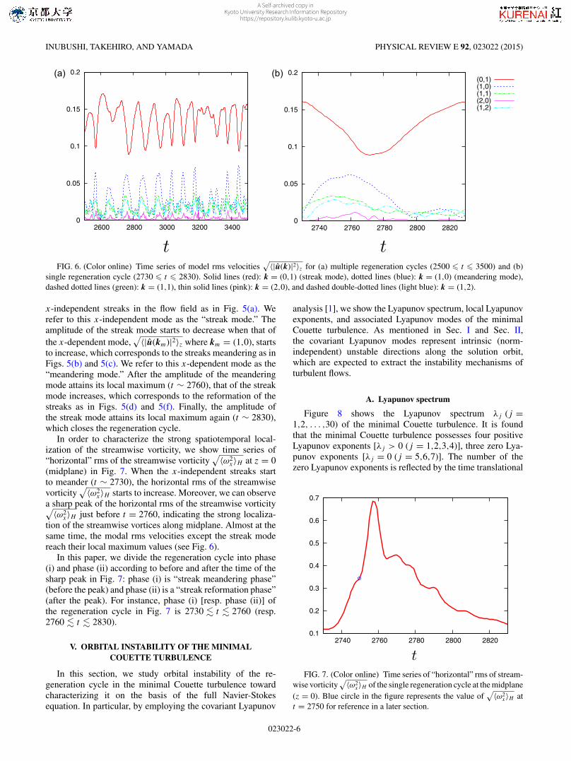
u(k,l,z) is the Fourier coefficient of the velocity field: u(k,z) =〈u(x,y,z)e−i(kxx+kyy)〉H (kx = αk,ky = βl). Hereafter we dropthe z dependence of u(k,z) as u(k) for simplicity. Figure 6shows time series of the modal rms velocities for (a) multi-ple regeneration cycles (2500 � t � 3500) and (b) a singleregeneration cycle (2730 � t � 2830), where solid lines (red)show k = (0,1), dotted lines (blue) show k = (1,0), dasheddotted lines (green) show k = (1,1), thin solid lines (pink)show k = (2,0), and dashed double-dotted lines (light blue)show k = (1,2). As reported by Hamilton et al. [12], the modalrms velocities oscillate nearly periodically and the period ofthe oscillation Tcycle is Tcycle � 100.
The time series in Fig. 6(b) corresponds to those of theregeneration cycle shown in Fig. 5. At the initial stage of theregeneration cycle (t ∼ 2730), the amplitude of x-independentmode is
√〈|u(ks)|2〉z where ks = (0,1) is the local maximum
in the cycle, which corresponds to the predominance of the
023022-5
A Self-archived copy inKyoto University Research Information Repository
https://repository.kulib.kyoto-u.ac.jp
INUBUSHI, TAKEHIRO, AND YAMADA PHYSICAL REVIEW E 92, 023022 (2015)
0
0.05
0.1
0.15
0.2
2600 2800 3000 3200 3400 0
0.05
0.1
0.15
0.2
2740 2760 2780 2800 2820
(0,1)(1,0)(1,1)(2,0)(1,2)
(a) (b)
FIG. 6. (Color online) Time series of model rms velocities√〈|u(k)|2〉z for (a) multiple regeneration cycles (2500 � t � 3500) and (b)
single regeneration cycle (2730 � t � 2830). Solid lines (red): k = (0,1) (streak mode), dotted lines (blue): k = (1,0) (meandering mode),dashed dotted lines (green): k = (1,1), thin solid lines (pink): k = (2,0), and dashed double-dotted lines (light blue): k = (1,2).
x-independent streaks in the flow field as in Fig. 5(a). Werefer to this x-independent mode as the “streak mode.” Theamplitude of the streak mode starts to decrease when that ofthe x-dependent mode,
√〈|u(km)|2〉z where km = (1,0), starts
to increase, which corresponds to the streaks meandering as inFigs. 5(b) and 5(c). We refer to this x-dependent mode as the“meandering mode.” After the amplitude of the meanderingmode attains its local maximum (t ∼ 2760), that of the streakmode increases, which corresponds to the reformation of thestreaks as in Figs. 5(d) and 5(f). Finally, the amplitude ofthe streak mode attains its local maximum again (t ∼ 2830),which closes the regeneration cycle.
In order to characterize the strong spatiotemporal local-ization of the streamwise vorticity, we show time series of“horizontal” rms of the streamwise vorticity
√〈ω2x〉H at z = 0
(midplane) in Fig. 7. When the x-independent streaks startto meander (t ∼ 2730), the horizontal rms of the streamwisevorticity
√〈ω2x〉H starts to increase. Moreover, we can observe
a sharp peak of the horizontal rms of the streamwise vorticity√〈ω2x〉H just before t = 2760, indicating the strong localiza-
tion of the streamwise vortices along midplane. Almost at thesame time, the modal rms velocities except the streak modereach their local maximum values (see Fig. 6).
In this paper, we divide the regeneration cycle into phase(i) and phase (ii) according to before and after the time of thesharp peak in Fig. 7: phase (i) is “streak meandering phase”(before the peak) and phase (ii) is a “streak reformation phase”(after the peak). For instance, phase (i) [resp. phase (ii)] ofthe regeneration cycle in Fig. 7 is 2730 � t � 2760 (resp.2760 � t � 2830).
V. ORBITAL INSTABILITY OF THE MINIMALCOUETTE TURBULENCE
In this section, we study orbital instability of the re-generation cycle in the minimal Couette turbulence towardcharacterizing it on the basis of the full Navier-Stokesequation. In particular, by employing the covariant Lyapunov
analysis [1], we show the Lyapunov spectrum, local Lyapunovexponents, and associated Lyapunov modes of the minimalCouette turbulence. As mentioned in Sec. I and Sec. II,the covariant Lyapunov modes represent intrinsic (norm-independent) unstable directions along the solution orbit,which are expected to extract the instability mechanisms ofturbulent flows.
A. Lyapunov spectrum
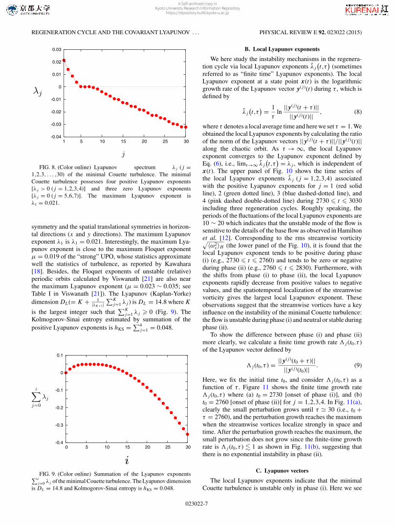
Figure 8 shows the Lyapunov spectrum λj (j =1,2, . . . ,30) of the minimal Couette turbulence. It is foundthat the minimal Couette turbulence possesses four positiveLyapunov exponents [λj > 0 (j = 1,2,3,4)], three zero Lya-punov exponents [λj = 0 (j = 5,6,7)]. The number of thezero Lyapunov exponents is reflected by the time translational
0.1
0.2
0.3
0.4
0.5
0.6
0.7
2740 2760 2780 2800 2820
FIG. 7. (Color online) Time series of “horizontal” rms of stream-wise vorticity
√〈ω2x〉H of the single regeneration cycle at the midplane
(z = 0). Blue circle in the figure represents the value of√〈ω2
x〉H att = 2750 for reference in a later section.
023022-6
A Self-archived copy inKyoto University Research Information Repository
https://repository.kulib.kyoto-u.ac.jp
REGENERATION CYCLE AND THE COVARIANT LYAPUNOV . . . PHYSICAL REVIEW E 92, 023022 (2015)
-0.04
-0.03
-0.02
-0.01
0
0.01
0.02
0.03
5 10 15 20 25 30 1
FIG. 8. (Color online) Lyapunov spectrum λj (j =1,2,3, . . . ,30) of the minimal Couette turbulence. The minimalCouette turbulence possesses four positive Lyapunov exponents[λj > 0 (j = 1,2,3,4)] and three zero Lyapunov exponents[λj = 0 (j = 5,6,7)]. The maximum Lyapunov exponent isλ1 = 0.021.
symmetry and the spatial translational symmetries in horizon-tal directions (x and y directions). The maximum Lyapunovexponent λ1 is λ1 = 0.021. Interestingly, the maximum Lya-punov exponent is close to the maximum Floquet exponentμ = 0.019 of the “strong” UPO, whose statistics approximatewell the statistics of turbulence, as reported by Kawahara[18]. Besides, the Floquet exponents of unstable (relative)periodic orbits calculated by Viswanath [21] are also nearthe maximum Lyapunov exponent (μ = 0.023 ∼ 0.035; seeTable I in Viswanath [21]). The Lyapunov (Kaplan-Yorke)dimension DL(= K + 1
|λK+1|∑K
j=1 λj ) is DL = 14.8 where K
is the largest integer such that∑K
j=1 λj � 0 (Fig. 9). TheKolmogorov-Sinai entropy estimated by summation of thepositive Lyapunov exponents is hKS = ∑4
j=1 = 0.048.
-0.4
-0.3
-0.2
-0.1
0
0.1
0 5 10 15 20 25 30
FIG. 9. (Color online) Summation of the Lyapunov exponents∑i
j=0 λj of the minimal Couette turbulence. The Lyapunov dimensionis DL = 14.8 and Kolmogorov-Sinai entropy is hKS = 0.048.
B. Local Lyapunov exponents
We here study the instability mechanisms in the regenera-tion cycle via local Lyapunov exponents λj
(t,τ
)(sometimes
referred to as “finite time” Lyapunov exponents). The localLyapunov exponent at a state point x(t) is the logarithmicgrowth rate of the Lyapunov vector y(j )(t) during τ , which isdefined by
λj
(t,τ
) = 1
τln
|| y(j )(t + τ )|||| y(j )(t)|| , (8)
where τ denotes a local average time and here we set τ = 1. Weobtained the local Lyapunov exponents by calculating the ratioof the norm of the Lyapunov vectors || y(j )(t + τ )||/|| y(j )(t)||along the chaotic orbit. As τ → ∞, the local Lyapunovexponent converges to the Lyapunov exponent defined byEq. (6), i.e., limτ→∞ λj
(t,τ
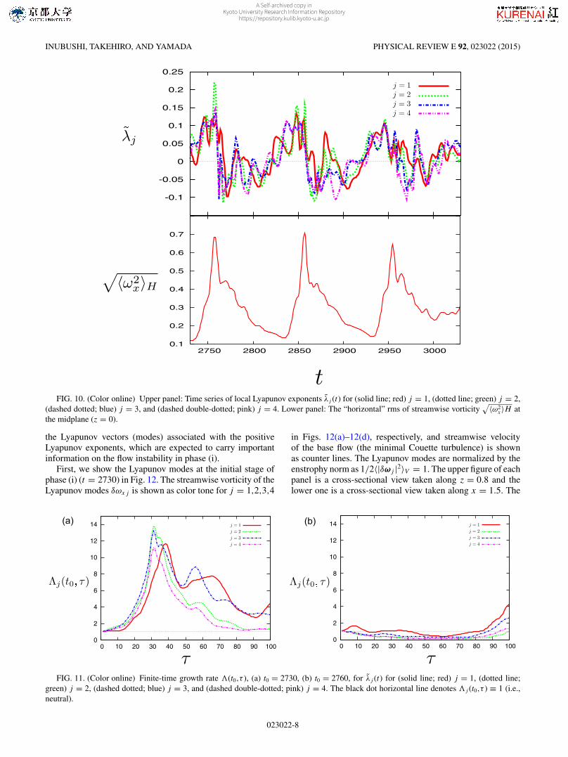
) = λj , which is independent ofx(t). The upper panel of Fig. 10 shows the time series ofthe local Lyapunov exponents λj (j = 1,2,3,4) associatedwith the positive Lyapunov exponents for j = 1 (red solidline), 2 (green dotted line), 3 (blue dashed-dotted line), and4 (pink dashed double-dotted line) during 2730 � t � 3030including three regeneration cycles. Roughly speaking, theperiods of the fluctuations of the local Lyapunov exponents are10 ∼ 20 which indicates that the unstable mode of the flow issensitive to the details of the base flow as observed in Hamiltonet al. [12]. Corresponding to the rms streamwise vorticity√〈ω2
x〉H (the lower panel of the Fig. 10), it is found that thelocal Lyapunov exponent tends to be positive during phase(i) (e.g., 2730 � t � 2760) and tends to be zero or negativeduring phase (ii) (e.g., 2760 � t � 2830). Furthermore, withthe shifts from phase (i) to phase (ii), the local Lyapunovexponents rapidly decrease from positive values to negativevalues, and the spatiotemporal localization of the streamwisevorticity gives the largest local Lyapunov exponent. Theseobservations suggest that the streamwise vortices have a keyinfluence on the instability of the minimal Couette turbulence:the flow is unstable during phase (i) and neutral or stable duringphase (ii).
To show the difference between phase (i) and phase (ii)more clearly, we calculate a finite time growth rate �j (t0,τ )of the Lyapunov vector defined by
�j (t0,τ ) = || y(j )(t0 + τ )|||| y(j )(t0)|| . (9)
Here, we fix the initial time t0, and consider �j (t0,τ ) as afunction of τ . Figure 11 shows the finite time growth rate�j (t0,τ ) where (a) t0 = 2730 [onset of phase (i)], and (b)t0 = 2760 [onset of phase (ii)] for j = 1,2,3,4. In Fig. 11(a),clearly the small perturbation grows until τ � 30 (i.e., t0 +τ = 2760), and the perturbation growth reaches the maximumwhen the streamwise vortices localize strongly in space andtime. After the perturbation growth reaches the maximum, thesmall perturbation does not grow since the finite-time growthrate is �j (t0,τ ) � 1 as shown in Fig. 11(b), suggesting thatthere is no exponential instability in phase (ii).
C. Lyapunov vectors
The local Lyapunov exponents indicate that the minimalCouette turbulence is unstable only in phase (i). Here we see
023022-7
A Self-archived copy inKyoto University Research Information Repository
https://repository.kulib.kyoto-u.ac.jp
INUBUSHI, TAKEHIRO, AND YAMADA PHYSICAL REVIEW E 92, 023022 (2015)
-0.1
-0.05
0
0.05
0.1
0.15
0.2
0.25
0.1
0.2
0.3
0.4
0.5
0.6
0.7
2750 2800 2850 2900 2950 3000
FIG. 10. (Color online) Upper panel: Time series of local Lyapunov exponents λj (t) for (solid line; red) j = 1, (dotted line; green) j = 2,(dashed dotted; blue) j = 3, and (dashed double-dotted; pink) j = 4. Lower panel: The “horizontal” rms of streamwise vorticity
√〈ω2x〉H at
the midplane (z = 0).
the Lyapunov vectors (modes) associated with the positiveLyapunov exponents, which are expected to carry importantinformation on the flow instability in phase (i).
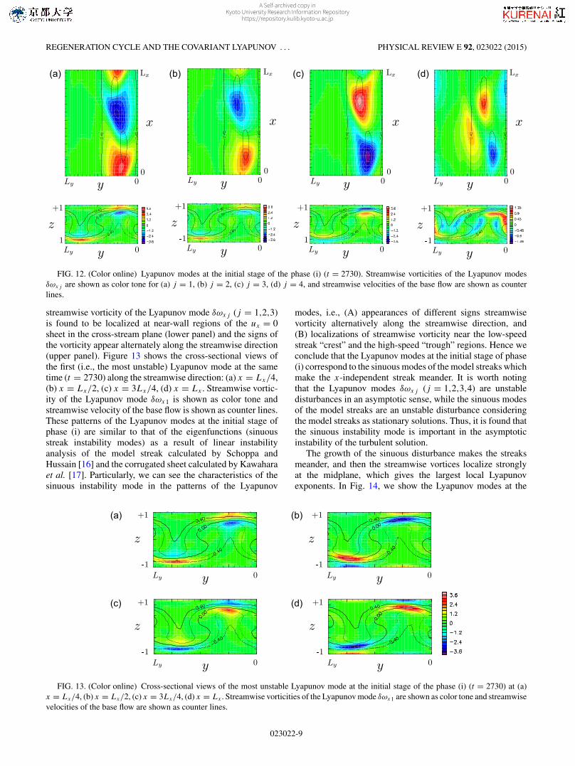
First, we show the Lyapunov modes at the initial stage ofphase (i) (t = 2730) in Fig. 12. The streamwise vorticity of theLyapunov modes δωxj is shown as color tone for j = 1,2,3,4
in Figs. 12(a)–12(d), respectively, and streamwise velocityof the base flow (the minimal Couette turbulence) is shownas counter lines. The Lyapunov modes are normalized by theenstrophy norm as 1/2〈|δωj |2〉V = 1. The upper figure of eachpanel is a cross-sectional view taken along z = 0.8 and thelower one is a cross-sectional view taken along x = 1.5. The
0
2
4
6
8
10
12
14
0 10 20 30 40 50 60 70 80 90 100 0
2
4
6
8
10
12
14
0 10 20 30 40 50 60 70 80 90 100
(a) (b)
FIG. 11. (Color online) Finite-time growth rate �(t0,τ ), (a) t0 = 2730, (b) t0 = 2760, for λj (t) for (solid line; red) j = 1, (dotted line;green) j = 2, (dashed dotted; blue) j = 3, and (dashed double-dotted; pink) j = 4. The black dot horizontal line denotes �j (t0,τ ) ≡ 1 (i.e.,neutral).
023022-8
A Self-archived copy inKyoto University Research Information Repository
https://repository.kulib.kyoto-u.ac.jp
REGENERATION CYCLE AND THE COVARIANT LYAPUNOV . . . PHYSICAL REVIEW E 92, 023022 (2015)
(a) (b) (c) (d)
FIG. 12. (Color online) Lyapunov modes at the initial stage of the phase (i) (t = 2730). Streamwise vorticities of the Lyapunov modesδωxj are shown as color tone for (a) j = 1, (b) j = 2, (c) j = 3, (d) j = 4, and streamwise velocities of the base flow are shown as counterlines.
streamwise vorticity of the Lyapunov mode δωxj (j = 1,2,3)is found to be localized at near-wall regions of the ux = 0sheet in the cross-stream plane (lower panel) and the signs ofthe vorticity appear alternately along the streamwise direction(upper panel). Figure 13 shows the cross-sectional views ofthe first (i.e., the most unstable) Lyapunov mode at the sametime (t = 2730) along the streamwise direction: (a) x = Lx/4,(b) x = Lx/2, (c) x = 3Lx/4, (d) x = Lx . Streamwise vortic-ity of the Lyapunov mode δωx1 is shown as color tone andstreamwise velocity of the base flow is shown as counter lines.These patterns of the Lyapunov modes at the initial stage ofphase (i) are similar to that of the eigenfunctions (sinuousstreak instability modes) as a result of linear instabilityanalysis of the model streak calculated by Schoppa andHussain [16] and the corrugated sheet calculated by Kawaharaet al. [17]. Particularly, we can see the characteristics of thesinuous instability mode in the patterns of the Lyapunov
modes, i.e., (A) appearances of different signs streamwisevorticity alternatively along the streamwise direction, and(B) localizations of streamwise vorticity near the low-speedstreak “crest” and the high-speed “trough” regions. Hence weconclude that the Lyapunov modes at the initial stage of phase(i) correspond to the sinuous modes of the model streaks whichmake the x-independent streak meander. It is worth notingthat the Lyapunov modes δωxj (j = 1,2,3,4) are unstabledisturbances in an asymptotic sense, while the sinuous modesof the model streaks are an unstable disturbance consideringthe model streaks as stationary solutions. Thus, it is found thatthe sinuous instability mode is important in the asymptoticinstability of the turbulent solution.
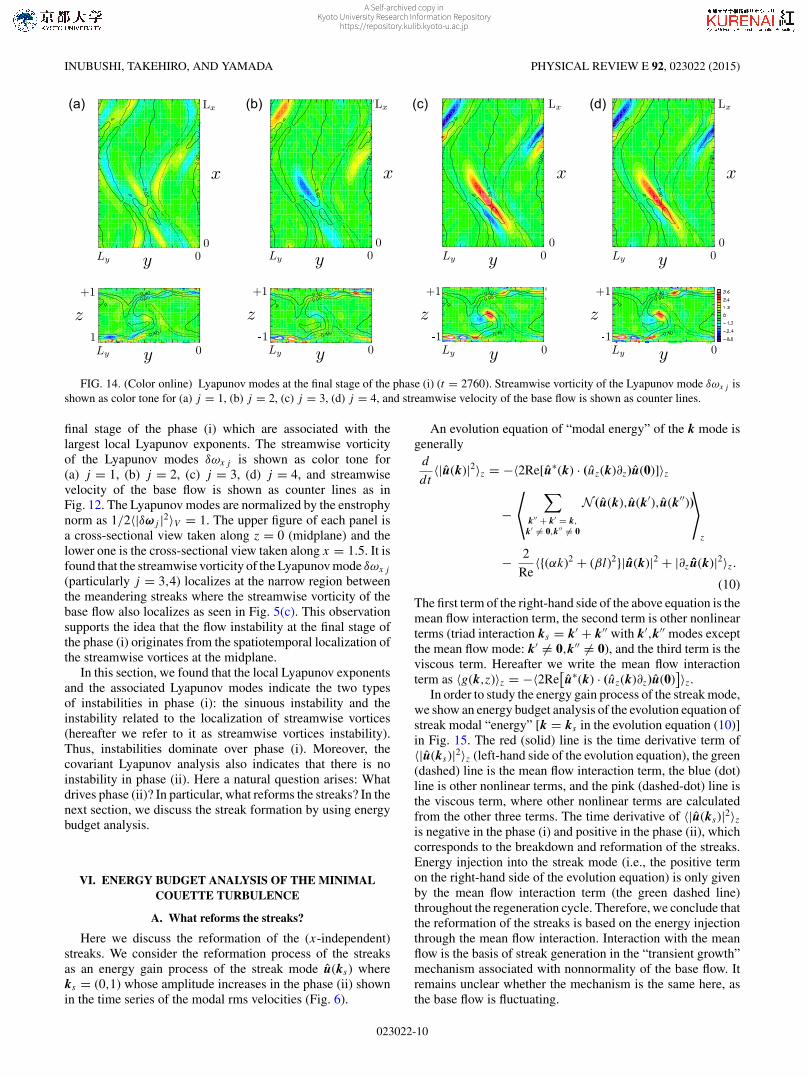
The growth of the sinuous disturbance makes the streaksmeander, and then the streamwise vortices localize stronglyat the midplane, which gives the largest local Lyapunovexponents. In Fig. 14, we show the Lyapunov modes at the
(a) (b)
(c) (d)
FIG. 13. (Color online) Cross-sectional views of the most unstable Lyapunov mode at the initial stage of the phase (i) (t = 2730) at (a)x = Lx/4, (b) x = Lx/2, (c) x = 3Lx/4, (d) x = Lx . Streamwise vorticities of the Lyapunov mode δωx1 are shown as color tone and streamwisevelocities of the base flow are shown as counter lines.
023022-9
A Self-archived copy inKyoto University Research Information Repository
https://repository.kulib.kyoto-u.ac.jp
INUBUSHI, TAKEHIRO, AND YAMADA PHYSICAL REVIEW E 92, 023022 (2015)
(a) (b) (c) (d)
FIG. 14. (Color online) Lyapunov modes at the final stage of the phase (i) (t = 2760). Streamwise vorticity of the Lyapunov mode δωxj isshown as color tone for (a) j = 1, (b) j = 2, (c) j = 3, (d) j = 4, and streamwise velocity of the base flow is shown as counter lines.
final stage of the phase (i) which are associated with thelargest local Lyapunov exponents. The streamwise vorticityof the Lyapunov modes δωxj is shown as color tone for(a) j = 1, (b) j = 2, (c) j = 3, (d) j = 4, and streamwisevelocity of the base flow is shown as counter lines as inFig. 12. The Lyapunov modes are normalized by the enstrophynorm as 1/2〈|δωj |2〉V = 1. The upper figure of each panel isa cross-sectional view taken along z = 0 (midplane) and thelower one is the cross-sectional view taken along x = 1.5. It isfound that the streamwise vorticity of the Lyapunov mode δωxj
(particularly j = 3,4) localizes at the narrow region betweenthe meandering streaks where the streamwise vorticity of thebase flow also localizes as seen in Fig. 5(c). This observationsupports the idea that the flow instability at the final stage ofthe phase (i) originates from the spatiotemporal localization ofthe streamwise vortices at the midplane.
In this section, we found that the local Lyapunov exponentsand the associated Lyapunov modes indicate the two typesof instabilities in phase (i): the sinuous instability and theinstability related to the localization of streamwise vortices(hereafter we refer to it as streamwise vortices instability).Thus, instabilities dominate over phase (i). Moreover, thecovariant Lyapunov analysis also indicates that there is noinstability in phase (ii). Here a natural question arises: Whatdrives phase (ii)? In particular, what reforms the streaks? In thenext section, we discuss the streak formation by using energybudget analysis.
VI. ENERGY BUDGET ANALYSIS OF THE MINIMALCOUETTE TURBULENCE
A. What reforms the streaks?
Here we discuss the reformation of the (x-independent)streaks. We consider the reformation process of the streaksas an energy gain process of the streak mode u(ks) whereks = (0,1) whose amplitude increases in the phase (ii) shownin the time series of the modal rms velocities (Fig. 6).
An evolution equation of “modal energy” of the k mode isgenerallyd
dt〈|u(k)|2〉z = −〈2Re[u∗(k) · (uz(k)∂z)u(0)]〉z
−˝ ∑
k′′ + k′ = k,
k′ �= 0,k′′ �= 0
N (u(k),u(k′),u(k′′))˛
z
− 2
Re〈{(αk)2 + (βl)2}|u(k)|2 + |∂zu(k)|2〉z.
(10)
The first term of the right-hand side of the above equation is themean flow interaction term, the second term is other nonlinearterms (triad interaction ks = k′ + k′′ with k′,k′′ modes exceptthe mean flow mode: k′ �= 0,k′′ �= 0), and the third term is theviscous term. Hereafter we write the mean flow interactionterm as 〈g(k,z)〉z = −〈2Re
[u∗(k) · (uz(k)∂z)u(0)
]〉z.In order to study the energy gain process of the streak mode,
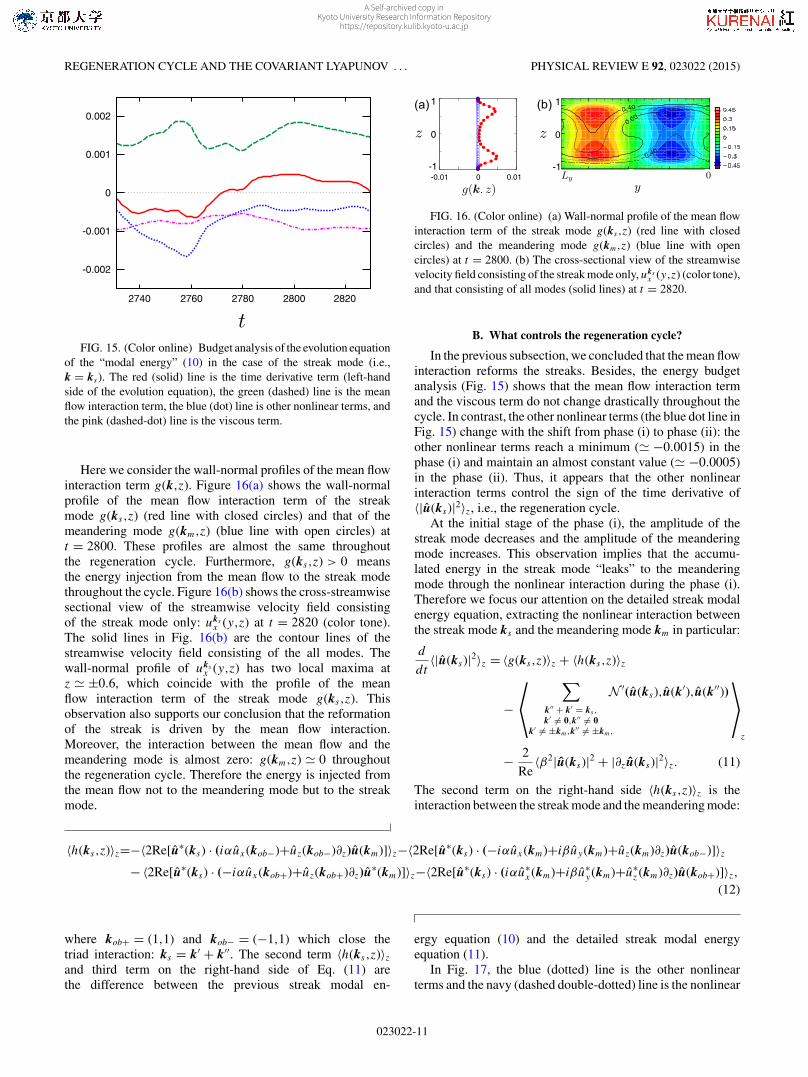
we show an energy budget analysis of the evolution equation ofstreak modal “energy” [k = ks in the evolution equation (10)]in Fig. 15. The red (solid) line is the time derivative term of〈|u(ks)|2〉z (left-hand side of the evolution equation), the green(dashed) line is the mean flow interaction term, the blue (dot)line is other nonlinear terms, and the pink (dashed-dot) line isthe viscous term, where other nonlinear terms are calculatedfrom the other three terms. The time derivative of 〈|u(ks)|2〉zis negative in the phase (i) and positive in the phase (ii), whichcorresponds to the breakdown and reformation of the streaks.Energy injection into the streak mode (i.e., the positive termon the right-hand side of the evolution equation) is only givenby the mean flow interaction term (the green dashed line)throughout the regeneration cycle. Therefore, we conclude thatthe reformation of the streaks is based on the energy injectionthrough the mean flow interaction. Interaction with the meanflow is the basis of streak generation in the “transient growth”mechanism associated with nonnormality of the base flow. Itremains unclear whether the mechanism is the same here, asthe base flow is fluctuating.
023022-10
A Self-archived copy inKyoto University Research Information Repository
https://repository.kulib.kyoto-u.ac.jp
REGENERATION CYCLE AND THE COVARIANT LYAPUNOV . . . PHYSICAL REVIEW E 92, 023022 (2015)
-0.002
-0.001
0
0.001
0.002
2740 2760 2780 2800 2820
FIG. 15. (Color online) Budget analysis of the evolution equationof the “modal energy” (10) in the case of the streak mode (i.e.,k = ks). The red (solid) line is the time derivative term (left-handside of the evolution equation), the green (dashed) line is the meanflow interaction term, the blue (dot) line is other nonlinear terms, andthe pink (dashed-dot) line is the viscous term.
Here we consider the wall-normal profiles of the mean flowinteraction term g(k,z). Figure 16(a) shows the wall-normalprofile of the mean flow interaction term of the streakmode g(ks ,z) (red line with closed circles) and that of themeandering mode g(km,z) (blue line with open circles) att = 2800. These profiles are almost the same throughoutthe regeneration cycle. Furthermore, g(ks ,z) > 0 meansthe energy injection from the mean flow to the streak modethroughout the cycle. Figure 16(b) shows the cross-streamwisesectional view of the streamwise velocity field consistingof the streak mode only: uks
x (y,z) at t = 2820 (color tone).The solid lines in Fig. 16(b) are the contour lines of thestreamwise velocity field consisting of the all modes. Thewall-normal profile of uks
x (y,z) has two local maxima atz � ±0.6, which coincide with the profile of the meanflow interaction term of the streak mode g(ks ,z). Thisobservation also supports our conclusion that the reformationof the streak is driven by the mean flow interaction.Moreover, the interaction between the mean flow and themeandering mode is almost zero: g(km,z) � 0 throughoutthe regeneration cycle. Therefore the energy is injected fromthe mean flow not to the meandering mode but to the streakmode.
-1
0
1
-0.01 0 0.01
(a) (b)
0
1
-1
FIG. 16. (Color online) (a) Wall-normal profile of the mean flowinteraction term of the streak mode g(ks ,z) (red line with closedcircles) and the meandering mode g(km,z) (blue line with opencircles) at t = 2800. (b) The cross-sectional view of the streamwisevelocity field consisting of the streak mode only, uks
x (y,z) (color tone),and that consisting of all modes (solid lines) at t = 2820.
B. What controls the regeneration cycle?
In the previous subsection, we concluded that the mean flowinteraction reforms the streaks. Besides, the energy budgetanalysis (Fig. 15) shows that the mean flow interaction termand the viscous term do not change drastically throughout thecycle. In contrast, the other nonlinear terms (the blue dot line inFig. 15) change with the shift from phase (i) to phase (ii): theother nonlinear terms reach a minimum (� −0.0015) in thephase (i) and maintain an almost constant value (� −0.0005)in the phase (ii). Thus, it appears that the other nonlinearinteraction terms control the sign of the time derivative of〈|u(ks)|2〉z, i.e., the regeneration cycle.
At the initial stage of the phase (i), the amplitude of thestreak mode decreases and the amplitude of the meanderingmode increases. This observation implies that the accumu-lated energy in the streak mode “leaks” to the meanderingmode through the nonlinear interaction during the phase (i).Therefore we focus our attention on the detailed streak modalenergy equation, extracting the nonlinear interaction betweenthe streak mode ks and the meandering mode km in particular:
d
dt〈|u(ks)|2〉z = 〈g(ks ,z)〉z + 〈h(ks ,z)〉z
−
� ∑
k′′ + k′ = ks ,
k′ �= 0,k′′ �= 0k′ �= ±km,k′′ �= ±km,
N ′(u(ks),u(k′),u(k′′))�
z
− 2
Re〈β2|u(ks)|2 + |∂zu(ks)|2〉z. (11)
The second term on the right-hand side 〈h(ks ,z)〉z is theinteraction between the streak mode and the meandering mode:
〈h(ks ,z)〉z=−〈2Re[u∗(ks) · (iαux(kob−)+uz(kob−)∂z)u(km)]〉z−〈2Re[u∗(ks) · (−iαux(km)+iβuy(km)+uz(km)∂z)u(kob−)]〉z− 〈2Re[u∗(ks) · (−iαux(kob+)+uz(kob+)∂z)u∗(km)]〉z−〈2Re[u∗(ks) · (iαu∗
x(km)+iβu∗y(km)+u∗
z (km)∂z)u(kob+)]〉z,(12)
where kob+ = (1,1) and kob− = (−1,1) which close thetriad interaction: ks = k′ + k′′. The second term 〈h(ks ,z)〉zand third term on the right-hand side of Eq. (11) arethe difference between the previous streak modal en-
ergy equation (10) and the detailed streak modal energyequation (11).
In Fig. 17, the blue (dotted) line is the other nonlinearterms and the navy (dashed double-dotted) line is the nonlinear
023022-11
A Self-archived copy inKyoto University Research Information Repository
https://repository.kulib.kyoto-u.ac.jp
INUBUSHI, TAKEHIRO, AND YAMADA PHYSICAL REVIEW E 92, 023022 (2015)
-0.002
-0.001
0
0.001
0.002
2740 2760 2780 2800 2820
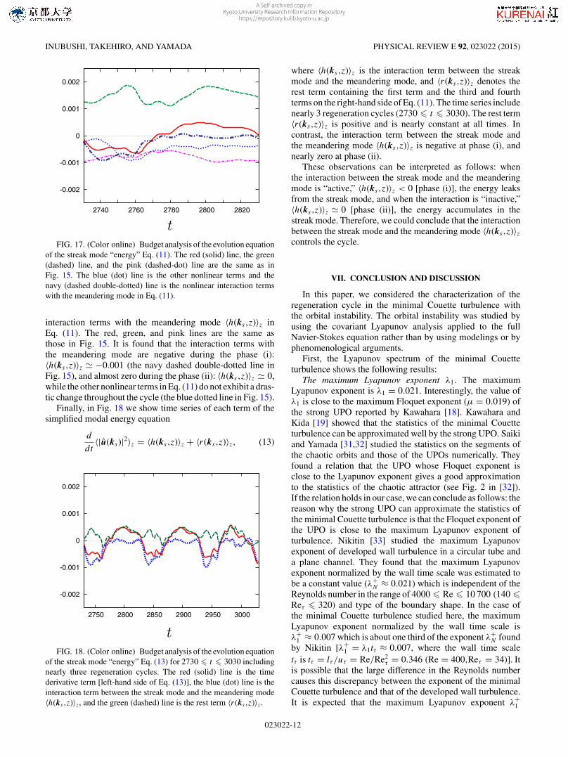
FIG. 17. (Color online) Budget analysis of the evolution equationof the streak mode “energy” Eq. (11). The red (solid) line, the green(dashed) line, and the pink (dashed-dot) line are the same as inFig. 15. The blue (dot) line is the other nonlinear terms and thenavy (dashed double-dotted) line is the nonlinear interaction termswith the meandering mode in Eq. (11).
interaction terms with the meandering mode 〈h(ks ,z)〉z inEq. (11). The red, green, and pink lines are the same asthose in Fig. 15. It is found that the interaction terms withthe meandering mode are negative during the phase (i):〈h(ks ,z)〉z � −0.001 (the navy dashed double-dotted line inFig. 15), and almost zero during the phase (ii): 〈h(ks ,z)〉z � 0,while the other nonlinear terms in Eq. (11) do not exhibit a dras-tic change throughout the cycle (the blue dotted line in Fig. 15).
Finally, in Fig. 18 we show time series of each term of thesimplified modal energy equation
d
dt〈|u(ks)|2〉z = 〈h(ks ,z)〉z + 〈r(ks ,z)〉z, (13)
-0.002
-0.001
0
0.001
0.002
2750 2800 2850 2900 2950 3000
FIG. 18. (Color online) Budget analysis of the evolution equationof the streak mode “energy” Eq. (13) for 2730 � t � 3030 includingnearly three regeneration cycles. The red (solid) line is the timederivative term [left-hand side of Eq. (13)], the blue (dot) line is theinteraction term between the streak mode and the meandering mode〈h(ks ,z)〉z, and the green (dashed) line is the rest term 〈r(ks ,z)〉z.
where 〈h(ks ,z)〉z is the interaction term between the streakmode and the meandering mode, and 〈r(ks ,z)〉z denotes therest term containing the first term and the third and fourthterms on the right-hand side of Eq. (11). The time series includenearly 3 regeneration cycles (2730 � t � 3030). The rest term〈r(ks ,z)〉z is positive and is nearly constant at all times. Incontrast, the interaction term between the streak mode andthe meandering mode 〈h(ks ,z)〉z is negative at phase (i), andnearly zero at phase (ii).
These observations can be interpreted as follows: whenthe interaction between the streak mode and the meanderingmode is “active,” 〈h(ks ,z)〉z < 0 [phase (i)], the energy leaksfrom the streak mode, and when the interaction is “inactive,”〈h(ks ,z)〉z � 0 [phase (ii)], the energy accumulates in thestreak mode. Therefore, we could conclude that the interactionbetween the streak mode and the meandering mode 〈h(ks ,z)〉zcontrols the cycle.
VII. CONCLUSION AND DISCUSSION
In this paper, we considered the characterization of theregeneration cycle in the minimal Couette turbulence withthe orbital instability. The orbital instability was studied byusing the covariant Lyapunov analysis applied to the fullNavier-Stokes equation rather than by using modelings or byphenomenological arguments.
First, the Lyapunov spectrum of the minimal Couetteturbulence shows the following results:
The maximum Lyapunov exponent λ1. The maximumLyapunov exponent is λ1 = 0.021. Interestingly, the value ofλ1 is close to the maximum Floquet exponent (μ = 0.019) ofthe strong UPO reported by Kawahara [18]. Kawahara andKida [19] showed that the statistics of the minimal Couetteturbulence can be approximated well by the strong UPO. Saikiand Yamada [31,32] studied the statistics on the segments ofthe chaotic orbits and those of the UPOs numerically. Theyfound a relation that the UPO whose Floquet exponent isclose to the Lyapunov exponent gives a good approximationto the statistics of the chaotic attractor (see Fig. 2 in [32]).If the relation holds in our case, we can conclude as follows: thereason why the strong UPO can approximate the statistics ofthe minimal Couette turbulence is that the Floquet exponent ofthe UPO is close to the maximum Lyapunov exponent ofturbulence. Nikitin [33] studied the maximum Lyapunovexponent of developed wall turbulence in a circular tube anda plane channel. They found that the maximum Lyapunovexponent normalized by the wall time scale was estimated tobe a constant value (λ+
N ≈ 0.021) which is independent of theReynolds number in the range of 4000 � Re � 10 700 (140 �Reτ � 320) and type of the boundary shape. In the case ofthe minimal Couette turbulence studied here, the maximumLyapunov exponent normalized by the wall time scale isλ+
1 ≈ 0.007 which is about one third of the exponent λ+N found
by Nikitin [λ+1 = λ1tτ ≈ 0.007, where the wall time scale
tτ is tτ = lτ /uτ = Re/Re2τ = 0.346 (Re = 400,Reτ = 34)]. It
is possible that the large difference in the Reynolds numbercauses this discrepancy between the exponent of the minimalCouette turbulence and that of the developed wall turbulence.It is expected that the maximum Lyapunov exponent λ+
1
023022-12
A Self-archived copy inKyoto University Research Information Repository
https://repository.kulib.kyoto-u.ac.jp
REGENERATION CYCLE AND THE COVARIANT LYAPUNOV . . . PHYSICAL REVIEW E 92, 023022 (2015)
(i) (ii)
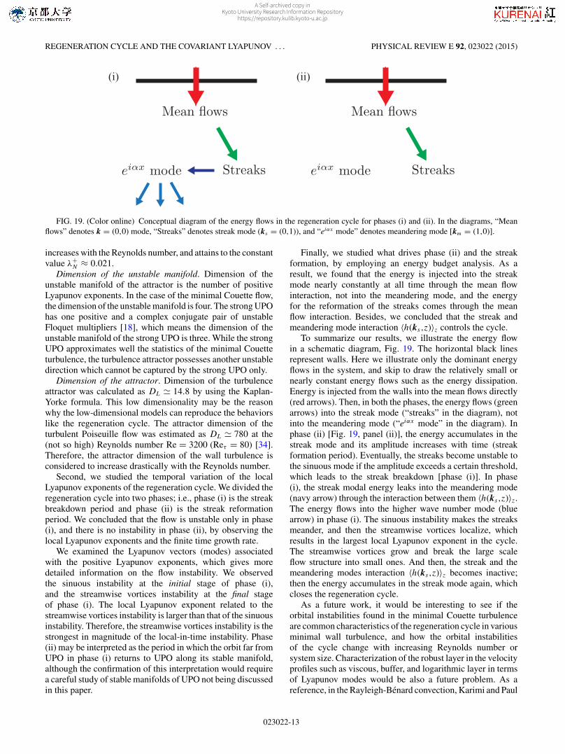
FIG. 19. (Color online) Conceptual diagram of the energy flows in the regeneration cycle for phases (i) and (ii). In the diagrams, “Meanflows” denotes k = (0,0) mode, “Streaks” denotes streak mode (ks = (0,1)), and “eiαx mode” denotes meandering mode [km = (1,0)].
increases with the Reynolds number, and attains to the constantvalue λ+
N ≈ 0.021.Dimension of the unstable manifold. Dimension of the
unstable manifold of the attractor is the number of positiveLyapunov exponents. In the case of the minimal Couette flow,the dimension of the unstable manifold is four. The strong UPOhas one positive and a complex conjugate pair of unstableFloquet multipliers [18], which means the dimension of theunstable manifold of the strong UPO is three. While the strongUPO approximates well the statistics of the minimal Couetteturbulence, the turbulence attractor possesses another unstabledirection which cannot be captured by the strong UPO only.
Dimension of the attractor. Dimension of the turbulenceattractor was calculated as DL � 14.8 by using the Kaplan-Yorke formula. This low dimensionality may be the reasonwhy the low-dimensional models can reproduce the behaviorslike the regeneration cycle. The attractor dimension of theturbulent Poiseuille flow was estimated as DL � 780 at the(not so high) Reynolds number Re = 3200 (Reτ = 80) [34].Therefore, the attractor dimension of the wall turbulence isconsidered to increase drastically with the Reynolds number.
Second, we studied the temporal variation of the localLyapunov exponents of the regeneration cycle. We divided theregeneration cycle into two phases; i.e., phase (i) is the streakbreakdown period and phase (ii) is the streak reformationperiod. We concluded that the flow is unstable only in phase(i), and there is no instability in phase (ii), by observing thelocal Lyapunov exponents and the finite time growth rate.
We examined the Lyapunov vectors (modes) associatedwith the positive Lyapunov exponents, which gives moredetailed information on the flow instability. We observedthe sinuous instability at the initial stage of phase (i),and the streamwise vortices instability at the final stageof phase (i). The local Lyapunov exponent related to thestreamwise vortices instability is larger than that of the sinuousinstability. Therefore, the streamwise vortices instability is thestrongest in magnitude of the local-in-time instability. Phase(ii) may be interpreted as the period in which the orbit far fromUPO in phase (i) returns to UPO along its stable manifold,although the confirmation of this interpretation would requirea careful study of stable manifolds of UPO not being discussedin this paper.
Finally, we studied what drives phase (ii) and the streakformation, by employing an energy budget analysis. As aresult, we found that the energy is injected into the streakmode nearly constantly at all time through the mean flowinteraction, not into the meandering mode, and the energyfor the reformation of the streaks comes through the meanflow interaction. Besides, we concluded that the streak andmeandering mode interaction 〈h(ks ,z)〉z controls the cycle.
To summarize our results, we illustrate the energy flowin a schematic diagram, Fig. 19. The horizontal black linesrepresent walls. Here we illustrate only the dominant energyflows in the system, and skip to draw the relatively small ornearly constant energy flows such as the energy dissipation.Energy is injected from the walls into the mean flows directly(red arrows). Then, in both the phases, the energy flows (greenarrows) into the streak mode (“streaks” in the diagram), notinto the meandering mode (“eiαx mode” in the diagram). Inphase (ii) [Fig. 19, panel (ii)], the energy accumulates in thestreak mode and its amplitude increases with time (streakformation period). Eventually, the streaks become unstable tothe sinuous mode if the amplitude exceeds a certain threshold,which leads to the streak breakdown [phase (i)]. In phase(i), the streak modal energy leaks into the meandering mode(navy arrow) through the interaction between them 〈h(ks ,z)〉z.The energy flows into the higher wave number mode (bluearrow) in phase (i). The sinuous instability makes the streaksmeander, and then the streamwise vortices localize, whichresults in the largest local Lyapunov exponent in the cycle.The streamwise vortices grow and break the large scaleflow structure into small ones. And then, the streak and themeandering modes interaction 〈h(ks ,z)〉z becomes inactive;then the energy accumulates in the streak mode again, whichcloses the regeneration cycle.
As a future work, it would be interesting to see if theorbital instabilities found in the minimal Couette turbulenceare common characteristics of the regeneration cycle in variousminimal wall turbulence, and how the orbital instabilitiesof the cycle change with increasing Reynolds number orsystem size. Characterization of the robust layer in the velocityprofiles such as viscous, buffer, and logarithmic layer in termsof Lyapunov modes would be also a future problem. As areference, in the Rayleigh-Benard convection, Karimi and Paul
023022-13
A Self-archived copy inKyoto University Research Information Repository
https://repository.kulib.kyoto-u.ac.jp
INUBUSHI, TAKEHIRO, AND YAMADA PHYSICAL REVIEW E 92, 023022 (2015)
[35] showed statistically that a transition from “boundary-dominated” dynamics to “bulk-dominated” dynamics occursas the system size is increased by employing the Lyapunovmode associated with the largest Lyapunov exponent.
In this paper, we studied the regeneration cycle only.However, as well as the regeneration cycle, the so-calledbursting event also occurs infrequently in wall turbulence,and is considered as an important phenomenon [24,36,37].It is challenging to characterize the bursting event from thestandpoint of the orbital instability and clarify the burstingmechanism. For instance, Kobayashi and Yamada [38] studiedintermittency in the GOY shell model and they characterizedthe bursting phenomenon in the GOY shell model with stableand unstable manifold structures via the covariant Lyapunov
analysis. It would also be interesting to study the burstingphenomenon in wall turbulence in terms of such manifoldstructures.
ACKNOWLEDGMENTS
This work was supported by JSPS KAKENHI Grants No.24340016, No. 15K13458, No. 22654014, No. 25610139,and No. 26103706 and by Grant-in-Aid for JSPS FellowsNo. 24-3995. The numerical calculations were performedon the computer systems of the Institute for InformationManagement and Communication (IIMC) of Kyoto Universityand of the Research Institute for Mathematical Sciences, KyotoUniversity.
[1] F. Ginelli, P. Poggi, A. Turchi, H. Chate, R. Livi, and A. Politi,Phys. Rev. Lett. 99, 130601 (2007).
[2] H.-L. Yang, K. A. Takeuchi, F. Ginelli, H. Chate, and G. Radons,Phys. Rev. Lett. 102, 074102 (2009).
[3] P. V. Kuptsov and S. P. Kuznetsov, Phys. Rev. E 80, 016205(2009).
[4] K. A. Takeuchi, H.-l. Yang, F. Ginelli, G. Radons, and H. Chate,Phys. Rev. E 84, 046214 (2011).
[5] M. Inubushi, M. U. Kobayashi, S.-i. Takehiro, and M. Yamada,Phys. Rev. E 85, 016331 (2012).
[6] M. Inubushi, M. U. Kobayashi, S. Takehiro, and M. Yamada,Procedia IUTAM 5, 244 (2012).
[7] H.-L. Yang and G. Radons, Phys. Rev. Lett. 108, 154101(2012).
[8] P. V. Kuptsov and U. Parlitz, J. Nonlinear Sci. 22, 727 (2012).[9] F. Ginelli, H. Chate, R. Livi, and A. Politi, J. Phys. A: Math.
Theor. 46, 254005 (2013).[10] G. Froyland, T. Huls, G. P. Morriss, and T. M. Watson, Physica
D 247, 18 (2013).[11] J. Jimenez and P. Moin, J. Fluid Mech. 225, 213 (1991).[12] J. M. Hamilton, J. Kim, and F. Waleffe, J. Fluid Mech. 287, 317
(1995).[13] R. L. Panton, Prog. Aerospace Sci. 37, 341 (2001).[14] T. Duriez, J.-L. Aider, and J. E. Wesfreid, Phys. Rev. Lett. 103,
144502 (2009).[15] F. Waleffe, Phys. Fluids 9, 883 (1997).[16] W. Schoppa and F. Hussain, J. Fluid Mech. 453, 57 (2002).[17] G. Kawahara, J. Jimenez, M. Uhlmann, and A. Pinelli, J. Fluid
Mech. 483, 315 (2003).[18] G. Kawahara, Fluid Dyn. Res. 41, 064001 (2009).
[19] G. Kawahara and G. Kida, J. Fluid Mech. 449, 291 (2001).[20] F. Waleffe, J. Fluid Mech. 435, 93 (2001).[21] D. Viswanath, J. Fluid Mech. 580, 339 (2007).[22] J. F. Gibson, J. Halcrow, and P. Cvitanovic, J. Fluid Mech. 611,
107 (2008).[23] J. Halcrow, J. F. Gibson, P. Cvitanovic, and D. Viswanath,
J. Fluid Mech. 621, 365 (2009).[24] L. van Veen and G. Kawahara, Phys. Rev. Lett. 107, 114501
(2011).[25] G. Kawahara, Annu. Rev. Fluid Mech. 44, 203 (2012).[26] J. Philip and P. Manneville, Phys. Rev. E 83, 036308 (2011).[27] K. Ishioka, ispack-0.95, http://www.gfd-dennou.org/arch/
ispack, GFD Dennou Club.[28] S. Takehiro, M. Odaka, K. Ishioka, M. Ishiwatari, and Y.
Hayashi, SPMODEL: A series of Hierarchical Spectral Modelsfor Geophysical Fluid Dynamics, Nagare Multimedia, 2006.Available online at http://www.nagare.or.jp/mm/2006/spmodel.
[29] See http://www.gfd-dennou.org/library/ruby.[30] I. Shimada and T. Nagashima, Prog. Theor. Phys. 61, 1605
(1979).[31] Y. Saiki and M. Yamada, Phys. Rev. E 79, 015201 (2009).[32] Y. Saiki and M. Yamada, RIMS Kokyuroku 1768, 143 (2011).[33] N. V. Nikitin, Fluid Dyn. 44, 652 (2009).[34] L. Keefe, P. Moin, and J. Kim, J. Fluid Mech. 242, 1 (1992).[35] A. Karimi and M. R. Paul, Phys. Rev. E 85, 046201 (2012).[36] T. Itano and S. Toh, J. Phys. Soc. Jpn. 70, 703 (2001).[37] J. Jimenez, G. Kawahara, M. P. Simens, M. Nagata, and M.
Shiba, Phys. Fluids 17, 015105 (2005).[38] M. U. Kobayashi and M. Yamada, J. Phys. A: Math. Theor. 46,
254008 (2013).
023022-14
A Self-archived copy inKyoto University Research Information Repository
https://repository.kulib.kyoto-u.ac.jp