departament d'arquitectura de computadors i sistemes ... · inyección de fallos que cambian...
TRANSCRIPT

Departament d'Arquitectura de
Computadors i Sistemes Operatius
Màster en Computació d'Altes Prestacions
2 0 0 9
Analyzing the
effects of transient
faults into
applications
Memoria del trabajo de investigación
del “Máster en Computación de Altas
Prestaciones”, realizada por João
Gramacho, bajo la dirección de Dolores
Rexachs presentada en la Escuela
Técnica Superior de Ingeniería
(Departamento de Arquitectura de
Computadores y Sistemas Operativos)

41746 - Iniciació a la recerca i treball fi de màster
Máster en Computación de Altas Prestaciones
Curso 2008-09
Analyzing the effects of transient faults into applications
Autor: João Gramacho
Director: Dolores Rexachs
Departamento Arquitectura de Computadores y Sistemas
Operativos
Escuela Técnica Superior de Ingeniería (ETSE)
Universidad Autónoma de Barcelona
Firmado
Autor Director
João Gramacho Dolores Rexachs

v
Acknowledgments
I am very thankful to the HP Labs team for the opportunity of
working with COTSon and for their patience in explaining how
those complex computers simulation stuff works. I also want to
thank the AMD SimNow team by their attention during the
development phase of this work.
I would like to thank all fellows of CAOS (always helping each
other), especially my working group (always helping each other
even more), and, in particular, I thank Dolores Rexachs and
Emilio Luque for their trust in my work.
Thank you, Dona Ana, Sérgio, Gabi, Anamel, Laís and all my
family and friends that, even far away, have always been by my
side.
To my friend Eduardo, that since 2004 was turning my dream of
being part of academic research into a real plan, for his support
in this first year living abroad.
Finally, I want to thank Graziela for her understanding, patience
and the motivation she gave me to finish this work.

vi

vii
Abstract
As computer chips implementation technologies evolve to obtain more performance, those
computer chips are using smaller components, with bigger density of transistors and working
with lower power voltages. All these factors turn the computer chips less robust and increase the
probability of a transient fault.
Transient faults may occur once and never more happen the same way in a computer system
lifetime. There are distinct consequences when a transient fault occurs: the operating system
might abort the execution if the change produced by the fault is detected by bad behavior of the
application, but the biggest risk is that the fault produces an undetected data corruption that
modifies the application final result without warnings (for example a bit flip in some crucial
data).
With the objective of researching transient faults in computer system’s processor registers and
memory we have developed an extension of HP’s and AMD joint full system simulation
environment, named COTSon. This extension allows the injection of faults that change a single
bit in processor registers and memory of the simulated computer.
The developed fault injection system makes it possible to: evaluate the effects of single bit flip
transient faults in an application, analyze an application robustness against single bit flip
transient faults and validate fault detection mechanism and strategies.
Key words: transient faults, fault injection, full system simulator.

viii
Resum
L'evolució dels processadors en cerca de millors prestacions fa que els xips duguin transistors
més petits i incloguin major quantitat y densitat de transistors, a més d'operar amb un voltatge
més baix. Tots aquests factors fan que els processadors siguin menys robusts i augmenten la
probabilitat de fallades transitòries.
Les fallades transitòries poden ocórrer una vegada i no tornar a passar de la mateixa forma en la
vida útil d'un sistema. Quan ocorren poden passar diferents conseqüències: el sistema operatiu
pot avortar l'execució quan el canvi produït per la fallada és detectat per mal comportament de
l'aplicació, però el risc major és que, amb el canvi produït, ocasioni una corrupció de dades que
no sigui detectada i canviï el resultat final de l'aplicació sense que ningú ho sàpiga.
Per a investigar sobre els efectes que les fallades transitòries poden ocasionar en els registres
d'un processador i en les memòries d'un computador, hem desenvolupat una extensió del
simulador d'ordinadors complet de HP (COTSon). L'extensió realitzada permet la injecció de
fallades que canvien un bit en registres i en les memòries del computador simulat.
La injecció de fallades permet: avaluar els efectes de les fallades transitòries que ocasionen el
canvi d'un bit en una aplicació, analitzar la robustesa d'una aplicació després de fallades
transitòries de canvis del valor d'un bit i validar mecanismes i estratègies de detecció de
fallades.
Paraules clau: Fallades transitòries, injecció de fallades, simulador d'ordinadors complet

ix
Resumen
La evolución de los procesadores en busca de prestaciones mejores hace que los circuitos lleven
transistores más pequeños e incluyan mayor cantidad y densidad de transistores, además de
operar con un voltaje menor. Todos estos factores hacen que los procesadores sean menos
robustos y aumenta la probabilidad de fallos transitorios.
Los fallos transitorios pueden ocurrir una vez y no volver a pasar, de la misma forma, en la vida
útil de un sistema. Cuando ocurren, pueden pasar distintas consecuencias: el sistema operativo
puede abortar la ejecución cuando el cambio producido por el fallo es detectado por mal
comportamiento de la aplicación, pero el riesgo mayor es que, con el cambio producido, se
produzca una corrupción de datos que no sea detectada y cambie el resultado final de la
aplicación sin que sea detectado.
Para investigar sobre los efectos que los fallos transitorios pueden ocasionar en los registros de
un procesador y en las memorias de un computador, hemos desarrollado una extensión del
simulador de ordenadores completo de HP (COTSon). La extensión realizada permite la
inyección de fallos que cambian un bit en registros y en las memorias del computador simulado.
La inyección de fallos permite: evaluar los efectos de los fallos transitorios que ocasionan
cambio de un bit en una aplicación, analizar la robustez de una aplicación tras fallos transitorios
de cambios del valor de un bit y validar mecanismos y estrategias de detección de fallos.
Palabras clave: Fallos transitorios, inyección de fallos, simulador de ordenadores completo.

x

xi
Contents
Chapter 1 Introduction ............................................................................................................... 1
1.1 Introduction ................................................................................................................... 1
1.2 Objective ....................................................................................................................... 2
1.3 Organization of this dissertation.................................................................................... 2
Chapter 2 Transient faults .......................................................................................................... 5
2.1 What is a transient fault? ............................................................................................... 5
2.2 The faults effect ............................................................................................................. 6
2.3 Metrics used in transient faults studies.......................................................................... 6
2.4 Evidence of soft errors .................................................................................................. 8
2.5 Possible outcomes of a transient fault ........................................................................... 9
2.6 Possible outcomes of soft errors .................................................................................. 11
2.6.1 Invalid instruction exception ............................................................................... 11
2.6.2 Parity error during read cycle .............................................................................. 12
2.6.3 Memory access violation ..................................................................................... 13
2.6.4 Change on a value ............................................................................................... 13
2.7 Studying transient faults .............................................................................................. 13
Chapter 3 Fault injection .......................................................................................................... 15
3.1 Introduction ................................................................................................................. 15
3.2 Fault injection tools main requirements ...................................................................... 15
3.3 Fault injection techniques ............................................................................................ 16
3.3.1 Physical fault injection ........................................................................................ 17
3.3.2 Fault emulation .................................................................................................... 17
3.3.3 Hardware emulation ............................................................................................ 18
3.3.4 Software simulation ............................................................................................. 18
3.4 Fault injection level of abstraction .............................................................................. 19
3.5 The environment type selected to our design .............................................................. 19
Chapter 4 Full system simulator .............................................................................................. 21
4.1 Introduction ................................................................................................................. 21
4.2 COTSon ....................................................................................................................... 21
4.2.1 COTSon configuration file .................................................................................. 22
Chapter 5 The fault injection framework ................................................................................. 25
5.1 Introduction ................................................................................................................. 25
5.2 WWW ......................................................................................................................... 25
5.2.1 Fault trigger (when) ............................................................................................. 25
xii
5.2.2 Fault location (where) ......................................................................................... 26
5.2.3 Fault operation (what) ......................................................................................... 26
5.3 The implementation of the fault injection framework ................................................. 26
5.3.1 Fault triggers ....................................................................................................... 27
5.3.2 Fault locations ..................................................................................................... 28
5.3.3 Fault operations ................................................................................................... 29
5.3.4 Using LUA .......................................................................................................... 30
5.4 How the framework works .......................................................................................... 31
5.5 Logging all information about the fault injection ....................................................... 32
Chapter 6 Experimental evaluation .......................................................................................... 35
6.1 Introduction ................................................................................................................. 35
6.2 Validation of the fault injection framework ................................................................ 38
6.3 Analyze the fault propagation in an application .......................................................... 38
6.3.1 Generating correct result ..................................................................................... 40
6.3.2 Generating system detected condition and incorrect result ................................. 41
6.3.3 Experiment conclusions ...................................................................................... 41
6.4 Analyze an application robustness .............................................................................. 41
6.4.1 Experiment setup ................................................................................................. 42
6.4.2 Experiment results ............................................................................................... 43
6.4.3 Experiment conclusions ...................................................................................... 44
6.5 Test fault detection mechanisms ................................................................................. 45
6.5.1 Experiment setup ................................................................................................. 46
6.5.2 Experiment results ............................................................................................... 46
6.5.3 Experiment conclusions ...................................................................................... 50
6.6 Analyzing all non-deterministic experiments together................................................ 51
Chapter 7 Conclusion and future work .................................................................................... 53
7.1 Conclusion ................................................................................................................... 53
7.2 Future work ................................................................................................................. 54
References ................................................................................................................................... 55

xiii
List of figures
Figure 1 – Radiation particle strike. .............................................................................................. 5
Figure 2 – Fault, error and failure states. ...................................................................................... 6
Figure 3 – Metrics and its relationships. ....................................................................................... 7
Figure 4 – Evidence of soft errors. ................................................................................................ 8
Figure 5 – Example IBM Power 4 hypothetical supercomputer MTTF. ...................................... 9
Figure 6 – Classification of possible outcomes of a transient fault. ............................................ 10
Figure 7 – Possible outcomes of soft errors. ............................................................................... 11
Figure 8 – Difference between "jump if grater" and "jump if less or equal" instructions. .......... 12
Figure 9 – Hardware-based and software based fault injection techniques. ............................... 16
Figure 10 – COTSon's architecture. ............................................................................................ 22
Figure 11 – A four CPU computer system memory hierarchy. ................................................... 22
Figure 12 – Described four CPU memory hierarchy. ................................................................. 23
Figure 13 – Programming language based four CPU memory hierarchy. .................................. 24
Figure 14 – When, where, what. ................................................................................................. 27
Figure 15 – Headers of the base classes of the fault injection framework. ................................. 27
Figure 16 – A fault injection description using LUA. ................................................................. 30
Figure 17 – How the framework works....................................................................................... 31
Figure 18 – Logging the fault injection initialization parameters. .............................................. 32
Figure 19 – Operation and location standard logging. ................................................................ 33
Figure 20 – Dump of processor registers and state. .................................................................... 33
Figure 21 – Possible results of a simulation with fault injection. ............................................... 35
Figure 22 – Simulated computer interconnection architecture in SimNow. ............................... 37
Figure 23 – Simulated computer memory hierarchy in COTSon................................................ 37
Figure 24 – Fault injection framework logging for validation. ................................................... 38
Figure 25 – The computational part of the matrix multiplication application............................. 39
Figure 26 – Assembly dump of the computational part of the application ................................. 40
Figure 27 – Fault injection simulation outcomes. ....................................................................... 44
Figure 28 – Per register simulation outcomes. ............................................................................ 44
Figure 29 – Per nibble simulation outcomes. .............................................................................. 44
Figure 30 – Duplication of the intermediate computation. ......................................................... 45
Figure 31 – Double verification of the conditional instructions.................................................. 45
Figure 32 – Computational part of the application changed to detect faults. .............................. 46
Figure 33 – Assembly code of the region where the SDC was produced. .................................. 47
Figure 34 – Fault injection simulation outcomes. ....................................................................... 48
Figure 35 – Per register simulation outcomes. ............................................................................ 48
Figure 36 – Per nibble simulation outcomes. .............................................................................. 48
Figure 37 – Fault injection simulation outcomes. ....................................................................... 49
Figure 38 – Per register simulation outcomes. ............................................................................ 50
Figure 39 – Per nibble simulation outcomes. .............................................................................. 50

xiv

xv
List of equations
Equation 1 – MTTF of a system. ................................................................................................... 7
Equation 2 – FIT of a system. ....................................................................................................... 7
Equation 3 – Relation between FIT and MTTF. ........................................................................... 7
Equation 4 – Amount of simulations per application compiled version. .................................... 42

xvi

xvii
List of tables
Table 1 – IBM Power 4 FIT per system effect. ............................................................................. 8
Table 2 – Implemented fault trigger classes. ............................................................................... 28
Table 3 – Implemented fault location classes. ............................................................................ 29
Table 4 – Implemented fault operation classes. .......................................................................... 30
Table 5 – Implemented debugging classes. ................................................................................. 33
Table 6 – X64 general purpose integer registers. ........................................................................ 42
Table 7 – All non-deterministic experiment results. ................................................................... 51

xviii

1
Chapter 1 Introduction
1.1 Introduction
With the evolution of computer processors for better performance, computer chips are using
smaller components, having more transistors with higher density and operating at lower voltage.
All these factors turn computer processors less robust against transient faults [1].
Transient faults are those faults that might occur once and may not happen again the same way
in a system lifetime. Transient faults in computer systems may occur in processors, memory,
internal buses and devices, often resulting in an inversion of a bit state (i.e. single bit flip) on the
faulty location [2]. Transient faults in computer systems commonly are effect of cosmic
radiation, high operating temperature and variations in the power supply subsystem [3].
A transient fault may cause an application to misbehave (e.g. write into an invalid memory
position; attempt to execute an inexistent instruction). Such an misbehaved application will then
be abruptly interrupted by the operating system fail-stop mechanism. Nevertheless, the biggest
risk happens when the transient fault bit-flip causes an undetected data corruption, resulting in
an incorrect application final result that might not be ever noticed [4].
In High Performance Computing (HPC), the risk of having a transient fault grows with the
amount of computer processors working together [5]. So, the more computational power a HPC
system has by adding more processors, the bigger is the risk of an unnoticed data corruption
produced by a transient fault [6].
Research about transient faults started with computers in hostile environments like outer space
[7], but official reports of transient faults’ effects in large computer installations became public
since year 2000. Those reports evidence the risk of having transient fault in HPC because of its
large number of components working together. With the risk of having transient faults affecting
computation results, researchers needed the occurrence of those faults to study its effects and
also to test their work.
Since transient faults occur in a very unpredictable way, an environment with fault injection
capabilities is needed to study the effects of these faults in computers, operating systems and
applications [8].
There are different ways to inject faults depending on the purpose of the fault injection: to test
hardware robustness [3][9][10][11], to test applications on grid computing [12], test real-time
systems [13], to verify the effects on applications [14], to substitute physical fault injection [15]
and others but mostly to verify dependability of systems and applications [8]
[16][17][18][19][20].
To study the effects in applications of transient faults into computer system processors and
memory, these fault injections can be made by changing states of the processor registers or
changing data in memory, either randomly or based on a specific design, depending on the
purpose of injection.

2
To produce fault injections based on specific design and precision, it is necessary to have high
level control of the system in which faults are injected. Additionally is desired that the fault
injection didn’t influence the tested system more than producing the changes of the injected
fault [21], but we didn’t found an actual fault injection environment capable of using actual
operating systems (such as Linux or Windows) and applications, with full control of the
computer system tested and with low influence in the tested application.
In this master thesis we present an environment able to study transient faults effects into
simulated computer systems running actual operating systems and actual applications both
deterministically, with a very specific fault injection strategy, and non-deterministically, with
randomly configured fault injection strategies.
1.2 Objective
Our objective in this master thesis is to have an environment to help us to analyze the effects of
transient faults into applications. By designing this environment, we will be able to do fault
injection experiments to:
a) Evaluate the effects in applications of single bit flip transient faults into processor
registers and memory;
b) Analyze an application robustness against single bit flip transient faults on processor
registers and memory;
c) Test fault detection mechanisms.
A starting point of the environment designing is to define how to describe a way to reproduce
transient faults: when to reproduce, where to affect and what to change.
In order to evaluate the effects of transient faults in applications, we want to reproduce the
common outcomes handled by computer processors and operating systems using very specific
fault injection strategies. We also want to able to generate data corruption in the application.
In order to analyze an application robustness against transient faults, we want to do a fault
injection campaign using non-deterministic fault injection strategy. To enhance the analysis, as
the use of processor registers may change depending on compiler options to achieve more
performance, we also want to use the studied application compiled with and without compiler
optimizations and compare their outcomes.
To verify the effectiveness of a fault detection mechanism, we want to change an application
source code using a purely software based mechanism to hardening applications against
transient faults by duplicating the intermediate computation [22].
1.3 Organization of this dissertation
This dissertation contains seven chapters. In the next chapter, we present an overview about
transient faults, concepts related to transient faults research and explain why is important to
study about transient faults.
Chapter 3 describes common fault injection environment types, its characteristics and also
present related works. This chapter also explains the fault injection environment type selected to
design our purposed environment.
3
In Chapter 4 we present an overview about full system simulators and also present COTSon: the
full system simulator used to simulate the computer systems running the operating system and
the applications analyzed in this work.
Chapter 5 describes the implementation of the fault injection framework as an extension of the
COTSon full system simulator. This chapter also presents how we proposed the description of
the transient fault to be reproduced by the purposed environment and how we made the
integration with the full system simulator.
In Chapter 6 we validate the implementation of the fault injection framework and evaluate an
application according to the three main objectives of this work: evaluate the effects of transient
faults, analyze an application robustness against transient faults and test fault detection
mechanisms.
Finally, in Chapter 7 we state our conclusions and purpose some future works.

4
5
Chapter 2 Transient faults
2.1 What is a transient fault?
Transient faults are faults that do not reflect a permanent malfunction. A permanent fault in
some component will produce faults, errors or unexpected behavior every time this faulty
component is used. Transient faults, on the other hand, may occur only once on the whole
component lifetime because they are a result of external sources influences, such as high-energy
particles that cause voltage pulses in digital circuits, or some internal sources like power supply
noise and temperature variation, for example [1].
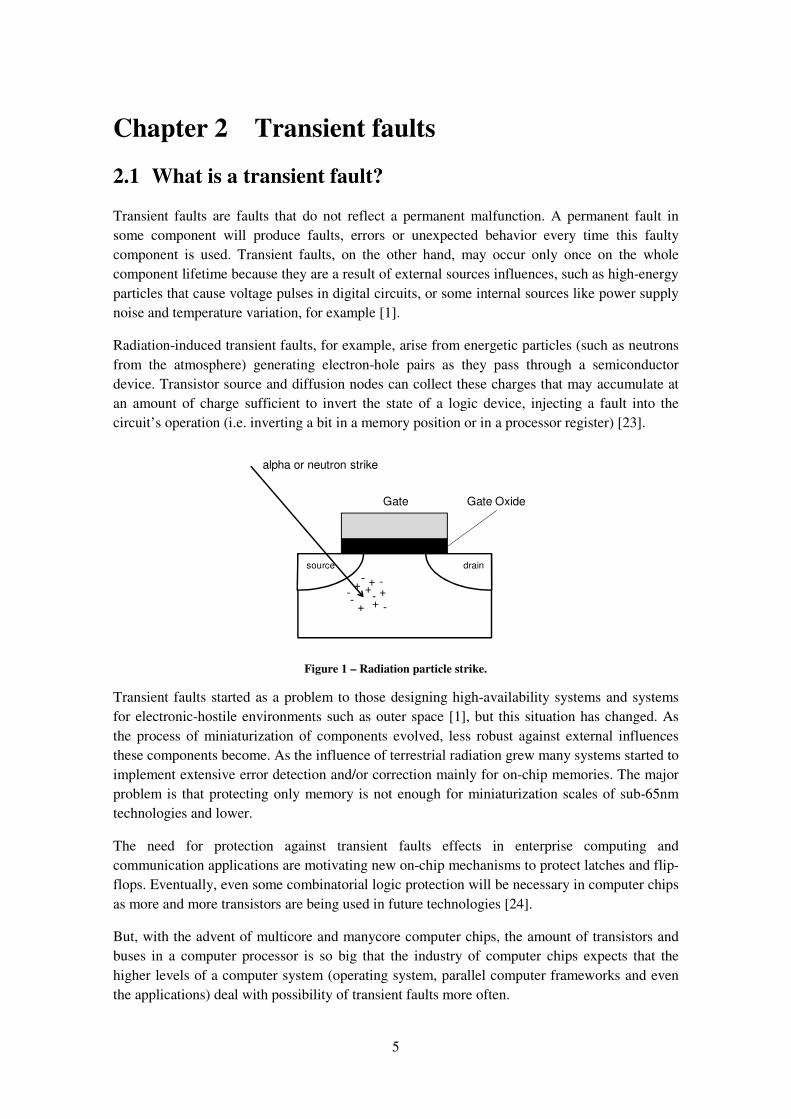
Radiation-induced transient faults, for example, arise from energetic particles (such as neutrons
from the atmosphere) generating electron-hole pairs as they pass through a semiconductor
device. Transistor source and diffusion nodes can collect these charges that may accumulate at
an amount of charge sufficient to invert the state of a logic device, injecting a fault into the
circuit’s operation (i.e. inverting a bit in a memory position or in a processor register) [23].
Figure 1 – Radiation particle strike.
Transient faults started as a problem to those designing high-availability systems and systems
for electronic-hostile environments such as outer space [1], but this situation has changed. As
the process of miniaturization of components evolved, less robust against external influences
these components become. As the influence of terrestrial radiation grew many systems started to
implement extensive error detection and/or correction mainly for on-chip memories. The major
problem is that protecting only memory is not enough for miniaturization scales of sub-65nm
technologies and lower.
The need for protection against transient faults effects in enterprise computing and
communication applications are motivating new on-chip mechanisms to protect latches and flip-
flops. Eventually, even some combinatorial logic protection will be necessary in computer chips
as more and more transistors are being used in future technologies [24].
But, with the advent of multicore and manycore computer chips, the amount of transistors and
buses in a computer processor is so big that the industry of computer chips expects that the
higher levels of a computer system (operating system, parallel computer frameworks and even
the applications) deal with possibility of transient faults more often.
Gate Gate Oxide
alpha or neutron strike
source drain
+-+
-+
-+
- +-
+ -
6
2.2 The faults effect
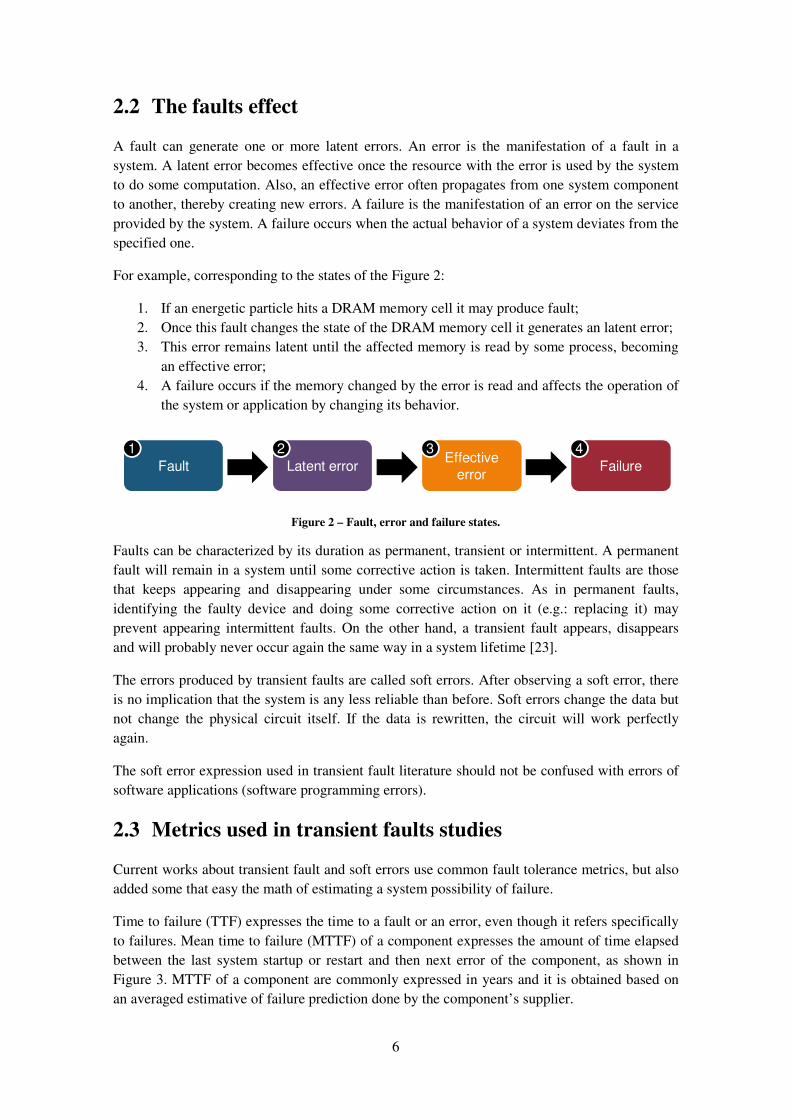
A fault can generate one or more latent errors. An error is the manifestation of a fault in a
system. A latent error becomes effective once the resource with the error is used by the system
to do some computation. Also, an effective error often propagates from one system component
to another, thereby creating new errors. A failure is the manifestation of an error on the service
provided by the system. A failure occurs when the actual behavior of a system deviates from the
specified one.
For example, corresponding to the states of the Figure 2:
1. If an energetic particle hits a DRAM memory cell it may produce fault;
2. Once this fault changes the state of the DRAM memory cell it generates an latent error;
3. This error remains latent until the affected memory is read by some process, becoming
an effective error;
4. A failure occurs if the memory changed by the error is read and affects the operation of
the system or application by changing its behavior.
Figure 2 – Fault, error and failure states.
Faults can be characterized by its duration as permanent, transient or intermittent. A permanent
fault will remain in a system until some corrective action is taken. Intermittent faults are those
that keeps appearing and disappearing under some circumstances. As in permanent faults,
identifying the faulty device and doing some corrective action on it (e.g.: replacing it) may
prevent appearing intermittent faults. On the other hand, a transient fault appears, disappears
and will probably never occur again the same way in a system lifetime [23].
The errors produced by transient faults are called soft errors. After observing a soft error, there
is no implication that the system is any less reliable than before. Soft errors change the data but
not change the physical circuit itself. If the data is rewritten, the circuit will work perfectly
again.
The soft error expression used in transient fault literature should not be confused with errors of
software applications (software programming errors).
2.3 Metrics used in transient faults studies
Current works about transient fault and soft errors use common fault tolerance metrics, but also
added some that easy the math of estimating a system possibility of failure.
Time to failure (TTF) expresses the time to a fault or an error, even though it refers specifically
to failures. Mean time to failure (MTTF) of a component expresses the amount of time elapsed
between the last system startup or restart and then next error of the component, as shown in
Figure 3. MTTF of a component are commonly expressed in years and it is obtained based on
an averaged estimative of failure prediction done by the component’s supplier.
Fault Latent errorEffective
errorFailure
1 2 3 4
7
The MTTF of a whole system (a group of components) can be obtained by combining the
MTTF of all its components, as shown in Equation 1 [23].
∑=
=
n
ii
0
system
MTTF
1
1MTTF
Equation 1 – MTTF of a system.
The use of the Failure In Time (FIT) term became more useful to engineers by its addictive
property. One FIT represent an error in a billion (910 ) hours. To compute a system FIT is only
necessary to add its components FIT, as shown in Equation 2 [23]:
∑=
=n
i isystem 0rate FITrate FIT
Equation 2 – FIT of a system.
FIT rate and MTTF of a component are inversely related under certain conditions:
days 365hours 24rate FIT
10yearsin MTTF
9
××
=
Equation 3 – Relation between FIT and MTTF.
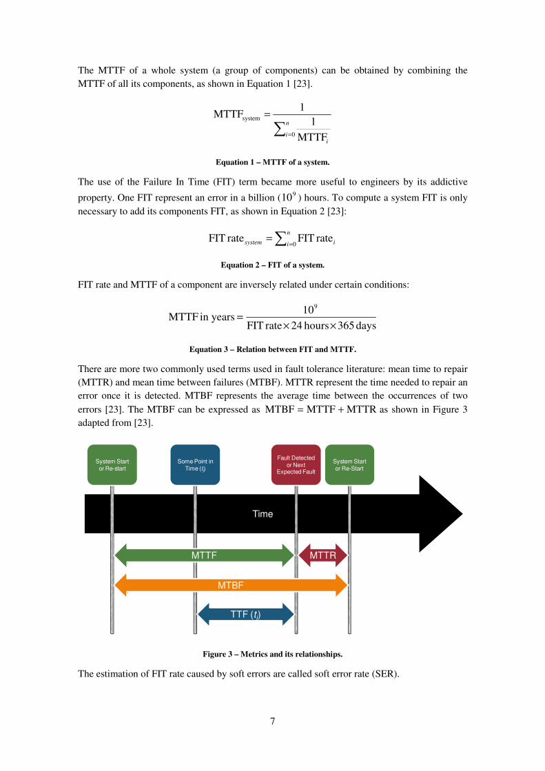
There are more two commonly used terms used in fault tolerance literature: mean time to repair
(MTTR) and mean time between failures (MTBF). MTTR represent the time needed to repair an
error once it is detected. MTBF represents the average time between the occurrences of two
errors [23]. The MTBF can be expressed as MTTRMTTFMTBF += as shown in Figure 3
adapted from [23].
Figure 3 – Metrics and its relationships.
The estimation of FIT rate caused by soft errors are called soft error rate (SER).
Time
System Start
or Re-start
Fault Detected
or Next Expected Fault
System Start
or Re-Start
MTTF MTTR
MTBF
Some Point in
Time (tj)
TTF (tj)

8
2.4 Evidence of soft errors
There are only few publications evidencing the occurrence of soft errors. As shown in Figure 4,
the first evidences of soft errors were caused by contamination in the chips production in late
70’s and 80’s.
Figure 4 – Evidence of soft errors.
Since 2000’s, the reports of soft errors in large computer installations such as supercomputers
and server farms are becoming more frequent. This happens because the number of components
in this kind of installations is very big (thousands of CPU and terabytes of memory). Also, in
this kind of installation it commonly has powerful and modern processors, with very high level
of miniaturization and high density of transistors (and potentially less robust against transient
faults).
For example, IBM has projected its Power 4 processor to be more robust against transient faults
than usual desktop processors. When usual desktop processors are supposed to have an MTTF
of 2 years, IBM Power 4 targets an MTTF of 7 years as shown in Table 1 [4].
Table 1 – IBM Power 4 FIT per system effect.
Even knowing that a seven years MTTF is a low probability of failure, when we start to analyze
this MTTF numbers in high performance computing, where we have hundreds or even
thousands of processors working together to solve a problem, the MTTF of an hypothetic
supercomputer lower as more processors are added, as show in Figure 5.
YEAR2
00
0
19
78
Intel first report:
Particle contamination
1986
IBM reported similar
problem with radioactive contamination
1984
IBM first report:
Cosmic radiation
2000
Sun Microsystems:
Transient faults in UltraSPARC-II SRAM chips
2004
Cypress:
Transient faults crashing a server farm
2005
HP:
2048 CPU HPC system crashed frequentlybecause of cosmic ray
strikes
19
80
19
90
2003
Cisco Systems:
Cisco 12000 line cards may reset after transient faults
FIT System effect Transient Fault Outcome MTTF (years)
114 Data corruption Silent Data Corruption 1000
4566 System-kill Detectable Unrecovered Error 25
11415 Process-kill Detectable Unrecovered Error 10
16095 7Total transient faults with some effect

9
Figure 5 – Example IBM Power 4 hypothetical supercomputer MTTF.
Soft errors in microprocessor logic will soon become more common. In particular, latches,
which are used in a variety of internal data structures, make up a large fraction of processor area
and are a potentially vulnerable part for transient faults [6].
Further, soft errors are a critical concern in the operation of real large systems. A 128k-node
BlueGene/L experiences one soft error in its L1 cache every 4-6 hours due to radioactive decay
in lead solder, the ASCI Q experienced 26.1 radiation induced CPU failures per week. A
similarly-sized Cray XD1 supercomputer is estimated to experience 109 soft errors per week in
CPUs, memory and FPGAs, if placed at the same altitude as the BlueGene/L [6].
2.5 Possible outcomes of a transient fault
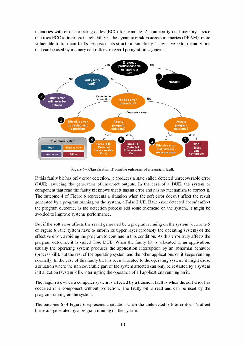
The Figure 6 was adapted from [4] and describes the possible outcomes of an energetic particle
hit in a computer processor or memory.
The outcome 1 of Figure 6 indicates that the energetic particle hit was not capable of generating
a fault.
The latent error happen when the energetic particle hit is capable of flipping a bit in a memory,
in a processor register or even in a latch used for some purpose.
If this faulty bit isn’t read by the system or it is overwritten at some point in time before using
the value changed by the fault, this latent error will never be noticed (outcome 2 of Figure 6).
When the faulty bit is read by the system or one of its components, the soft error becomes
effective.
The effective soft error can pass unnoticed by the upper layers of the component reading it if
this bit is protected with detection and correction (outcome 3 of Figure 6). This is the case of
3.727.866
931.966
232.992
58.248
14.562
3.640
910
228
57
14
1
10
100
1.000
10.000
100.000
1.000.000
10.000.000
1 4 16 64 256 1024 4096 16384 65536 262144
Min
ute
s
Processors
MTTF in minutes
10
memories with error-correcting codes (ECC) for example. A common type of memory device
that uses ECC to improve its reliability is the dynamic random access memories (DRAM), more
vulnerable to transient faults because of its structural simplicity. They have extra memory bits
that can be used by memory controllers to record parity of bit segments.
Figure 6 – Classification of possible outcomes of a transient fault.
If this faulty bit has only error detection, it produces a state called detected unrecoverable error
(DUE), avoiding the generation of incorrect outputs. In the case of a DUE, the system or
component that read the faulty bit knows that it has an error and has no mechanism to correct it.
The outcome 4 of Figure 6 represents a situation when the soft error doesn’t affect the result
generated by a program running on the system, a False DUE. If the error detected doesn’t affect
the program outcome, as the detection process add some overhead on the system, it might be
avoided to improve systems performance.
But if the soft error affects the result generated by a program running on the system (outcome 5
of Figure 6), the system have to inform its upper layer (probably the operating system) of the
effective error, avoiding the program to continue in this condition. As this error truly affects the
program outcome, it is called True DUE. When the faulty bit is allocated to an application,
usually the operating system produces the application interruption by an abnormal behavior
(process kill), but the rest of the operating system and the other applications on it keeps running
normally. In the case of this faulty bit has been allocated to the operating system, it might cause
a situation where the unrecoverable part of the system affected can only be restarted by a system
initialization (system kill), interrupting the operation of all applications running on it.
The major risk when a computer system is affected by a transient fault is when the soft error has
occurred in a component without protection. The faulty bit is read and can be used by the
program running on the system.
The outcome 6 of Figure 6 represents a situation when the undetected soft error doesn’t affect
the result generated by a program running on the system.
Faulty bit is read?
Bit has error protection?
Latent error will never be
noticed
Affects program
outcome?
Effective error corrected; not
a problem
Affects program
outcome?
Effective error not noticed;
not a problem
SDC(Silent
DataCorruption)
False DUE(Detected
Unrecoverable Error)
True DUE(Detected
Unrecoverable Error)
Energetic particle capable
of flipping a bit?
No fault
Color Classification
Fault
Latent error
Effective error
Failure
YES
YESNO NOYES
NO
NO
NO
YES
Detection only
Detection &correction
1
2
3
4 5 6 7
11
If the system uses the faulty bit in its operation without knowing that it was changed, this
system will have a silent data corruption (SDC), the most dangerous outcome of a transient
fault. The SDC (outcome 7 of Figure 6) will be processed by the application running on the
system or by the operating system and might cause unpredicted consequences on the overall
system behavior.
Currently, the industry specifies soft error rates of its components in terms of SDC and DUE
numbers. The total SER of a system or component can be expressed as a sum of its SDC FIT
and DUE FIT [23] as shown in Table 1 previously explained.
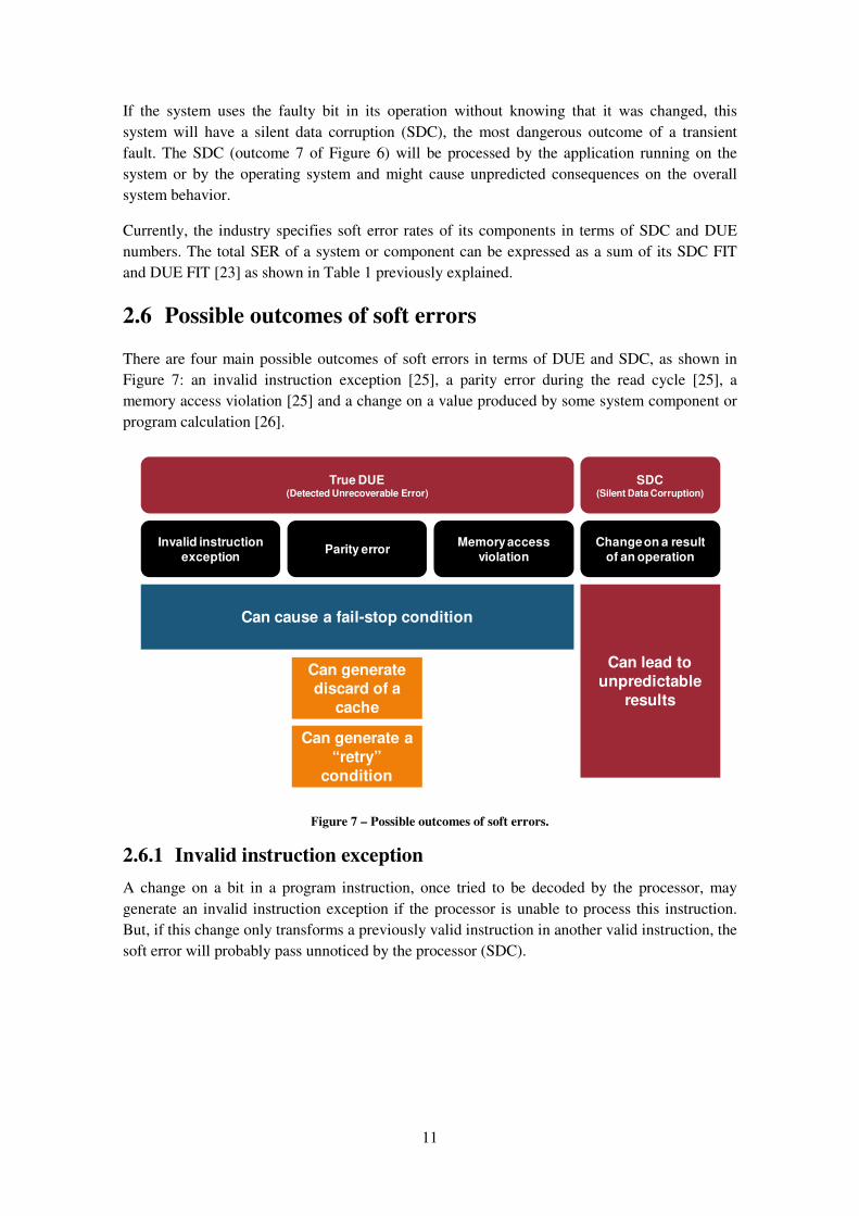
2.6 Possible outcomes of soft errors
There are four main possible outcomes of soft errors in terms of DUE and SDC, as shown in
Figure 7: an invalid instruction exception [25], a parity error during the read cycle [25], a
memory access violation [25] and a change on a value produced by some system component or
program calculation [26].
Figure 7 – Possible outcomes of soft errors.
2.6.1 Invalid instruction exception
A change on a bit in a program instruction, once tried to be decoded by the processor, may
generate an invalid instruction exception if the processor is unable to process this instruction.
But, if this change only transforms a previously valid instruction in another valid instruction, the
soft error will probably pass unnoticed by the processor (SDC).
Invalid instruction
exceptionParity error
Memory access
violation
Change on a result
of an operation
Can generate a
“retry”
condition
Can generate discard of a
cache
Can cause a fail-stop condition
Can lead to
unpredictable
results
SDC(Silent Data Corruption)
True DUE(Detected Unrecoverable Error)

12
Figure 8 – Difference between "jump if grater" and "jump if less or equal" instructions.
Even transforming a valid instruction in another valid instruction by changing a bit, it is
possible that the original instruction parameters in the bytes right after the instruction don’t fit
the fault generated instruction parameters, raising an invalid instruction exception.
Some processor architectures might be more vulnerable to changes in instructions than others.
In fact, for example, in the x86 architecture [27], the difference between a conditional jump
instruction where a tested value is greater than other and a conditional jump where a tested
value is less or equal other (inverse conditions) is only a bit, as shown in Figure 8.
2.6.2 Parity error during read cycle
A parity error generated by a transient fault may occur on memory devices (main computer
memory or caches) or in buses lines.
It is common that buses lines that implement parity check in transmissions also implement the
possibility of the retransmission of the affected portion of data. The effect of this situation on
computer systems is a small delay in the transmission, but the system keeps running normally.
When a soft error affects a memory position and the component affected uses parity to detect
such situation, the consequences of this error depends on where in the memory hierarchy is the
affected portion of memory.
If the parity error is in a portion of the main memory of the computer system it might be
possible to recover it in the following cases:
a) The operating system uses the virtual memory resources of the processor and has copy
of the affected portion of the memory stored in the swap file. If the portion affected
didn’t have been changed previously by normal computation, the operating system can
recover the affected page from the swap file, restoring the previously known state of it.
b) The affected portion of the memory is a code segment of an application and there are
binaries of the application in another device. In this case, is possible to the operating
system read again the application’s binaries on the other device and restore the affected
portion of the memory.
$01111111
$01111110

13
If there is no source of a possible copy of the affected portion of the memory, the operating
system has two options: stop the operation of the application or raise an error to the application,
allowing the application try to recover itself.
When the parity error is detected in a cache memory, the possible scenarios are very similar to
the previously explained when affected the main memory: if the portion of the cache memory
affected didn’t have been changed previously by normal computation, the memory controller
can ask for a new copy of it to the main memory (or to the upper cache level) and restore the
previously known state of it.
But, in the case of this portion of the cache memory has been changed by normal computation,
the operating system may stop the operation of the application or raise an error.
2.6.3 Memory access violation
A soft error affecting a memory pointer can make an application try to get or put data, or even to
jump into a memory space that isn’t valid in the application’s scope. Modern processors have
protection against this kind of behavior, raising access violation errors to the operating system.
Once noticed that an application is trying to access a memory location that doesn’t exist or is of
another process, the operating system stop the application execution avoiding propagating the
error to other parts of the system.
2.6.4 Change on a value
A single faulty bit is capable of generating a soft error that affect a component operation by
changing its expected result into an unexpected one.
This is the case of errors affecting internal processor components, for example. Registers,
pipeline, arithmetical logic unit (ALU), floating point unit (FPU), and almost all components of
a modern processor have some kind of memory portion (to store intermediary results of its
operations) and have some kind of buses to communicate to the other processor components.
All these auxiliary memories and internal buses are possible targets of a transient fault.
A soft error in an internal component of a processor may pass unnoticed in system’s operation if
the component didn’t have protection and if its result didn’t violate the application address-
space and didn’t produce an invalid operation.
The SDC, the most common effect in this kind of outcome of soft errors, won’t stop any
application execution and might only be noticed by the users if the final result generated by the
application differs significantly from the usual result.
2.7 Studying transient faults
The possibility of having unnoticed data corruption in applications execution leads the industry
to using very expensive computing environments to avoid this problem. By using triple modular
redundancy (executing every processor instruction in three different processors) and a voting
mechanism to verify if at least two of the results were equals, industries like banking institutions
can work with their application with almost no probable data corruption generated by transient
faults. But such expensive infrastructure is not feasible to everyone.

14
Processors designers are working more and more to obtain more performance of computer
processors and also they are explaining that they know about the growing trend of transient
faults but there are no major investment to solve this problem in processor architecture because
this probably implies in less processor performance, more circuitry to detect faults (and so more
processor area sensible to radiation) and more manufacturing costs. They are suggesting that the
upper levels (the operating system, application frameworks or even the application) should
know that faults may happen and should deal with this possibility.
To study about transient faults, their effects to deal with the upcoming problem informed by
computer processor designers, it is necessary to have an experimental environment capable of
reproducing the effects of transient faults in computer systems.

15
Chapter 3 Fault injection
3.1 Introduction
Fault injection is mostly used for system dependability evaluation [28]. It was by the need to
validate dependability properties of the fault tolerant systems that the research about fault
injection grew in importance [19].
A dependable computer system is capable of detect errors due to hardware or software faults,
isolate the errors cause (when possible) and recover from them [19]. In the case of the soft
errors, there is no need to isolate the errors cause because it is a transient situation that happened
sometime before the detection and probably won’t happen again the same way.
To obtain more confidence of the dependable properties of a system before its deployment is
important to do a validation by testing the system in the presence of faults.
As the faults expected by the system dependability properties may not happen often, it is a
common practice to put the system under testing (SUT) in fault injection campaigns. With fault
injection, the system under test can be evaluated in faulty conditions even if the real fault
doesn’t happen.
A fault injection campaign consists of a set of experiments on the target system with specific
workloads, injecting a specific fault (or set of faults) at specific trigger conditions. The target
system behavior can be monitored and information (such as results of application execution and
operating system logs) can be recorded as comprehensively as necessary and possible, to
understand and evaluate the effects of the injected faults [18].
3.2 Fault injection tools main requirements
There are four main features that a fault injection tool or environment should implement to
achieve the needs of those needing to inject faults into computer systems: be able to work with
multiple fault models, be able to setup multiple fault triggers, be able to target different
application models and to have versatile error reporting methods [29].
A fault injection tool or environment must be able to inject multiple fault models in its target
system. Bit-flips in processor’s registers, in memory used by the operating system kernel, in
applications virtual address space, in any physical memory address and I/O faults is some of
them.
A fault trigger is the condition expected by the fault injection tool to do the fault injection. It
might depend on the progress of the application under test (program counter), on time elapsed in
the test, on processor (and its registers) status and also on event-based triggers. As some fault
injection tools are used to test dependability on applications running on multiple computer
systems (such as clusters or grids), triggers based on event correlation of distinct nodes are a
very useful feature.
16
Fault injection campaigns can target a vast range of applications, such as distributed messaging
passing interface (MPI) applications, fault tolerance middleware and operating system
components. Also, those campaigns can be targeting some hardware prototypes or even
firmware implementations.
Extract information from a fault injection campaign and organize it to easily generate reports
and tracking information is also an important feature of a fault injection tool. Usually, those
fault injection campaigns have thousands of experiments to ensure that the most significant
situations of error where tested, generating a big amount of data to be analyzed.
There are also some desired requirements that we have selected because of its importance to the
transient fault research: reproducibility, fine graining, decoupling and low impact on target
application.
Every fault injection must be reproducible, even the non-deterministic ones. As a fault injection
campaign might have some unexpected results, the tool must be able to reproduce one specific
fault injection of the campaign, allowing the dependable system designers test its systems
detection/recovery features with a previously known injected fault.
It should be possible to inject faults for very specific cases (e.g. in a particular global state of the
application), even if it requires a better understanding of the tested application. With fine
graining it will be possible to test and observe very specific conditions during a fault injection
experiment.
Decoupling the fault injection platform from tested application is a desirable requirement too.
By injecting faults without source code modification of the tested application we could
guarantee that the fault injection tool didn’t change the application behavior (at least no more
than the fault injection itself).
The impact of the fault injection platform should be low. As some transient faults may affect
only the performance of an SUT, as lower as the impact of the fault injection platform in the
tested application more accurate can be possible working with fault injection without affecting
the tested application performance.
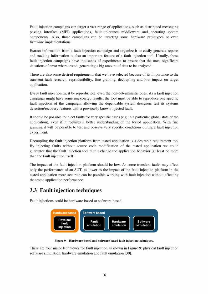
3.3 Fault injection techniques
Fault injections could be hardware-based or software-based.
Figure 9 – Hardware-based and software based fault injection techniques.
There are four major techniques for fault injection as shown in Figure 9: physical fault injection
software simulation, hardware emulation and fault emulation [30].
Hardware based Software based
Physical
fault injection
Software
simulation
Hardware
emulation
Fault
emulation

17
3.3.1 Physical fault injection
In the beginning of the studies about transient fault using fault injection, because of the nature
of the problem relative to energy particles striking processor and memories, the approach to do
the fault injection was using physical devices.
In the case of physical fault injection, the SUT is the actual tested fully functional computer
with its operating system and applications.
The fault injection device could be an electronic device that generates disturbances into
processor or memory pins or a device that exposes the SUT to radiation.
The problem with physical fault injection is that it is very unpredictable and probably
untraceable. Once made an injection, it is very difficult to verify what memory or part of the
processor was affected. Also, the necessary infrastructure to deal with physical fault injection
(like a radiation generator device) isn’t easy to obtain.
Perhaps, to test how shielded a computer system device is against radiation, for example, to
evaluate the computer system robustness in very hostile environments like the outer space, there
are space for physical fault injection campaigns.
For example, IBM has a published test with its Power 6 processor soft error tolerance using
proton irradiation [11]. In this analysis, the authors have listed the architectural characteristics
of IBM Power 6 processor and how those characteristics affect the robustness of the processor
against soft errors. The faults were injected using a proton beam and observing its effects using
an architectural verification program.
3.3.2 Fault emulation
In the case of the fault emulation, as in the case of the physical fault injection, the SUT is a fully
functional computer system.
Using processor and operating system debugging capabilities, the fault injector, usually a
concurrent software specially developed to this purpose, stops the execution of the application
being tested, do the fault injection by changing processor registers or the memory of the process
running the tested application and then let the process continue its operation.
One of the problems with the fault emulation approach is that the fault injector is a concurrent
process of the tested application. Because of this, it indirectly affects the application being
tested. As more complicated is the fault injection condition, tested frequently by the fault
injector to assure the correct moment to do the fault injection, more influence into the tested
application it generates.
A common approach using fault emulation is grid computing fault tolerance research, where in
major cases the fault injection is done by killing a working process after some time. A simple
operation (killing a process) with a simple trigger (after some time of application execution)
may not influence the application behavior significantly, but limit the scope of the fault
injection in transient faults studies.
For example, FAIL-FCI is a fault injection architecture designed for testing fault tolerance in
grid computing[12]. It is composed by three important parts: a compiler, that interprets the fault
injection scenario and generates a fault injection configuration file; a library, which distributes

18
the fault injection configuration file into the grid nodes; a daemon that interprets the fault
injection configuration file and compiles a fault injection tool specific for each grid node. The
fault injection scenario is described using FAIL, a language for fault description capable of
expressing complex and realistic fault scenarios.
3.3.3 Hardware emulation
Fault injection using hardware emulation is used when testing changes into processor and
memory hierarchy architecture.
In this case, an emulator of the desired architecture is used, and the SUT is a partial
implementation of a computer system, often without operating system, because those emulators
don’t perform to do full system emulation with actual operating system and actual applications.
Emulators based on VHDL models are used to propose techniques to let processors and memory
more robust against transient faults by changes in their internal architectures. The experiments
using those emulators and fault injection also often use precompiled benchmark applications
because of the difficulty to emulate an environment capable of compile actual applications.
For example, MEPHISTO is an environment for fault tolerance experiments based on VHDL
hardware description language [10]. MEPHISTO was designed to estimate the coverage of fault
tolerance mechanisms, to investigate different mechanisms for mapping results from one level
of abstraction to another and to validate fault and error models applied during fault injection
experiments. It uses changes into the VHDL model replacing some components to fault
injectable ones and interacts with the VHDL simulator to apply the fault injection.
3.3.4 Software simulation
The software simulation approach uses full system simulators to simulate a fully featured actual
computer system with all its components executing actual operating systems and applications.
In this case, the SUT is a simulated computer system with its operating system and applications.
As those full system simulators are fast enough to allow interactive execution, it is possible to
use a simulator to describe the SUT desired, install an actual operating system (like Linux or
Windows) into this simulated computer, install applications and frameworks into this operating
system.
As the fault injection using software simulation is done outside of the SUT, it doesn’t affect the
application being tested. The fault injector can stop the simulation, evaluate the trigger
condition, operate a fault injection and then restart the simulation. For the simulated computer
system is like the time didn’t stopped.
Dealing with a full system simulator implies that the fault injector can use lots of information to
evaluate fault trigger conditions: from processor registers state to memory hierarchy events, the
fault injector can even do a very detailed depuration of the fault injection conditions because it
won’t affect the tested application at all.

19
3.4 Fault injection level of abstraction
In addition to the method by which faults are injected, fault-injection techniques may also be
categorized by the level of abstraction at which the faults are injected. High level fault-detection
or fault-tolerant mechanisms may be verified by injecting faults at any lower level of abstraction
and allowing the errors to propagate to higher levels. In general, researchers prefer to inject
faults at the lowest levels to assure accuracy, the degree to which the injected faults reflect
actual faults. In practice, however, they are often forced to inject faults at higher levels to attain
a procedure that is tractable in terms of development cost and injection time.
3.5 The environment type selected to our design
By analyzing the current fault injection environment types and related works and also
evaluating common fault injection tools requirements with our objectives, we have selected to
use a software simulation with a full system simulator capable of simulating actual computer
architectures with actual operating systems and capable of running actual applications.
By using a full system simulator, we also could guarantee precision and accuracy in the fault
injection as we could have full control of the simulated computer.
Because of the nature of the computer system simulation, we can assume that a fault injection
environment added to a full system simulator will produce almost no impact into the tested
application, as the timing of the simulated computer can be manipulated by the simulator and
also because the fault injection mechanism will not be simulated with the tested application or
operating system.
About transparency, using a full system simulator with fault injection capabilities let us use
unchanged operating systems and applications. All the intelligence of the fault injection
mechanism is independent of adding code or changing the tested application.
Finally, by controlling the SUT using a full system simulator can let us generate very detailed
log information about what happens with the SUT during the simulation before and after an
injected fault.

20

21
Chapter 4 Full system simulator
4.1 Introduction
By the kind of transient fault research we desired, to use a full system simulator seemed to be a
good choice.
The complexity of computer system and cost constrains are turning simulators into a good
choice for design and analysis. Simulators are tools used by researchers, developers and system
designers to help understanding the impact of their decisions in a controlled environment that
can have its behavior extrapolated to real computer systems.
Computer system simulation in later 2004 had five important challenges: allow multiprocessor
and multithreaded simulation of operating systems and applications; improving sampling
techniques; achieve higher speeds instead of having a cycle-accurate simulation; possibility to
use representative and non-redundant benchmarks; increase the robustness of the simulation
methodology statistically to allow both independent validation and easy comparison between
simulators [31].
Computer system simulation can be decomposed in functional simulation and timing
simulation.
Functional simulators emulates the behavior of a target system (including operating system and
common devices) and normally is only concerned with functional correctness, giving an
imprecise notion of time on the simulated computer system.
Historically used to verify correctness of systems and do early software development, functional
simulators have recently become fast enough to approximate a native execution by using new
hypervisors and virtual machine characteristics of modern computer processors.
On the other hand, timing simulation is used to assess the performance of a computer system.
By adding latency to the operations of a functional simulator those timing simulators are
approximations of their real counterparts as absolute accuracy is not always necessary due to
high engineering costs.
Evaluating the full system simulators available and desiring to deal with simulation of high
performance computer systems we found COTSon. A full system simulator framework
developed by HP Labs and AMD, COTSon provides fast and accurate evaluation of current
computing systems, covering the full software stack and complete hardware models [32].
4.2 COTSon
COTSon is an x64 full system simulator able to simulate single core and manycore computer
systems running with actual operating systems (like Windows and Linux) and actual
applications.
COTSon extends the actual functionality of SimNow, AMD’s x64 functional simulator and it is
used to evaluate the functionality of the actual operating systems and applications in AMD
22
future processors. The simulator also helps in the development of BIOS to non-existing
processors before AMD have the real computer chip to test in a real computer.
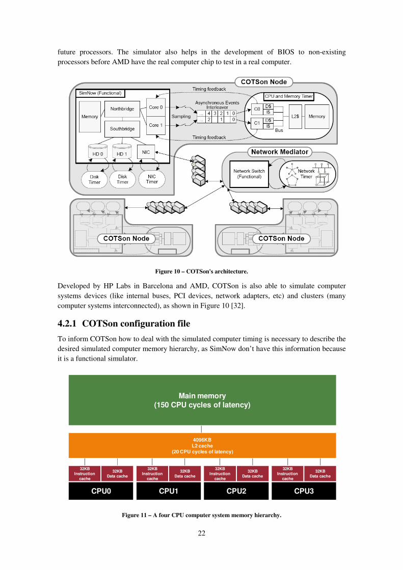
Figure 10 – COTSon's architecture.
Developed by HP Labs in Barcelona and AMD, COTSon is also able to simulate computer
systems devices (like internal buses, PCI devices, network adapters, etc) and clusters (many
computer systems interconnected), as shown in Figure 10 [32].
4.2.1 COTSon configuration file
To inform COTSon how to deal with the simulated computer timing is necessary to describe the
desired simulated computer memory hierarchy, as SimNow don’t have this information because
it is a functional simulator.
Figure 11 – A four CPU computer system memory hierarchy.
CPU0
32KB
Instruction
cache
32KB
Data cache
4096KBL2 cache
(20 CPU cycles of latency)
CPU1
32KB
Instruction
cache
32KB
Data cache
CPU2
32KB
Instruction
cache
32KB
Data cache
CPU3
32KB
Instruction
cache
32KB
Data cache
Main memory
(150 CPU cycles of latency)

23
In Figure 11 we show a hypothetic four CPU computer system memory hierarchy with latency
information for each level. The latencies are informed in CPU cycles and the latency for the
instruction and data caches of each CPU is zero.
Perhaps it should be possible to describe this memory hierarchy with some text syntax or even
XML, but the HP Labs team preferred to use LUA, a C++ like language, to describe the desired
simulation memory hierarchy and also every configuration aspects of the simulation.
With LUA it is possible to describe a computer memory hierarchy using a programming
language. The benefits of using a programming language are the possibility of using loops and
arithmetic in the simulated architecture description.
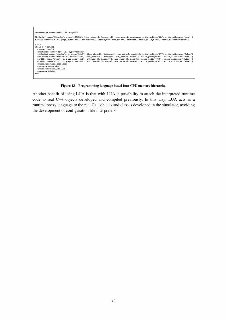
For example, to describe the memory hierarchy showed in Figure 11 it is possible to program a
loop to describe the processors memory hierarchy instead of describing each CPU memory
hierarchy alone, as can be seen comparing Figure 12 and Figure 13.
Figure 12 – Described four CPU memory hierarchy.
mem=Memory{ name="main", latency=150 }
l2=Cache{ name="l2cache", size="4096kB", line_size=16, latency=20, num_sets=4, next=mem, write_policy="WB", write_allocate="true" }
t2=TLB{ name="l2tlb", page_size="4kB", entries=512, latency=80, num_sets=4, next=mem, write_policy="WB", write_allocate="true" }
cpu=get_cpu(0)
cpu:timer{ name='cpu0', type="timer0” }
ic=Cache{ name="icache0", size="32kB", line_size=16, latency=0, num_sets=2, next=l2, write_policy="WT", write_allocate="false" }
dc=Cache{ name="dcache0", size="32kB", line_size=16, latency=0, num_sets=2, next=l2, write_policy="WT", write_allocate="false" }
it=TLB{ name="itlb0", page_size="4kB", entries=40, latency=0, num_sets=40, next=t2, write_policy="WT", write_allocate="false" }
dt=TLB{ name="dtlb0", page_size="4kB", entries=40, latency=0, num_sets=40, next=t2, write_policy="WT", write_allocate="false" }
cpu:instruction_cache(ic)
cpu:data_cache(dc)
cpu:instruction_tlb(it)
cpu:data_tlb(dt)
cpu=get_cpu(1)
cpu:timer{ name='cpu1', type="timer0” }
ic=Cache{ name="icache1", size="32kB", line_size=16, latency=0, num_sets=2, next=l2, write_policy="WT", write_allocate="false" }
dc=Cache{ name="dcache1", size="32kB", line_size=16, latency=0, num_sets=2, next=l2, write_policy="WT", write_allocate="false" }
it=TLB{ name="itlb1", page_size="4kB", entries=40, latency=0, num_sets=40, next=t2, write_policy="WT", write_allocate="false" }
dt=TLB{ name="dtlb1", page_size="4kB", entries=40, latency=0, num_sets=40, next=t2, write_policy="WT", write_allocate="false" }
cpu:instruction_cache(ic)
cpu:data_cache(dc)
cpu:instruction_tlb(it)
cpu:data_tlb(dt)
cpu=get_cpu(2)
cpu:timer{ name='cpu2', type="timer0” }
ic=Cache{ name="icache2", size="32kB", line_size=16, latency=0, num_sets=2, next=l2, write_policy="WT", write_allocate="false" }
dc=Cache{ name="dcache2", size="32kB", line_size=16, latency=0, num_sets=2, next=l2, write_policy="WT", write_allocate="false" }
it=TLB{ name="itlb2", page_size="4kB", entries=40, latency=0, num_sets=40, next=t2, write_policy="WT", write_allocate="false" }
dt=TLB{ name="dtlb2", page_size="4kB", entries=40, latency=0, num_sets=40, next=t2, write_policy="WT", write_allocate="false" }
cpu:instruction_cache(ic)
cpu:data_cache(dc)
cpu:instruction_tlb(it)
cpu:data_tlb(dt)
cpu=get_cpu(3)
cpu:timer{ name='cpu3', type="timer0” }
ic=Cache{ name="icache3", size="32kB", line_size=16, latency=0, num_sets=2, next=l2, write_policy="WT", write_allocate="false" }
dc=Cache{ name="dcache3", size="32kB", line_size=16, latency=0, num_sets=2, next=l2, write_policy="WT", write_allocate="false" }
it=TLB{ name="itlb3", page_size="4kB", entries=40, latency=0, num_sets=40, next=t2, write_policy="WT", write_allocate="false" }
dt=TLB{ name="dtlb3", page_size="4kB", entries=40, latency=0, num_sets=40, next=t2, write_policy="WT", write_allocate="false" }
cpu:instruction_cache(ic)
cpu:data_cache(dc)
cpu:instruction_tlb(it)
cpu:data_tlb(dt)
24
Figure 13 – Programming language based four CPU memory hierarchy.
Another benefit of using LUA is that with LUA is possibility to attach the interpreted runtime
code to real C++ objects developed and compiled previously. In this way, LUA acts as a
runtime proxy language to the real C++ objects and classes developed in the simulator, avoiding
the development of configuration file interpreters.
mem=Memory{ name="main", latency=150 }
l2=Cache{ name="l2cache", size="4096kB", line_size=16, latency=20, num_sets=4, next=mem, write_policy="WB", write_allocate="true" }
t2=TLB{ name="l2tlb", page_size="4kB", entries=512, latency=80, num_sets=4, next=mem, write_policy="WB", write_allocate="true" }
c = 0
while c < cpus()
cpu=get_cpu(c)
cpu:timer{ name='cpu'..c, type="timer0” }
ic=Cache{ name="icache"..c, size="32kB", line_size=16, latency=0, num_sets=2, next=l2, write_policy="WT", write_allocate="false"}
dc=Cache{ name="dcache".c, size="32kB", line_size=16, latency=0, num_sets=2, next=l2, write_policy="WT", write_allocate="false" }
it=TLB{ name="itlb"..c, page_size="4kB", entries=40, latency=0, num_sets=40, next=t2, write_policy="WT", write_allocate="false" }
dt=TLB{ name="dtlb"..c, page_size="4kB", entries=40, latency=0, num_sets=40, next=t2, write_policy="WT", write_allocate="false" }
cpu:instruction_cache(ic)
cpu:data_cache(dc)
cpu:instruction_tlb(it)
cpu:data_tlb(dt)
end

25
Chapter 5 The fault injection framework
5.1 Introduction
To achieve the objective of this master thesis, we have implemented a fault injection framework
into HP’s COTSon x64 full system simulator.
This fault injection framework added fault injection capabilities to COTSon, extending the
simulators purpose, as it can now be used also to evaluate de effects of transient-like faults into
processor registers and memory into applications.
Fully developed in C++, same programming language used in COTSon, our implementation
respects the COTSon coding style and also avoid the construction of structures that already
exists on COTSon.
5.2 WWW
A fault injection using our framework needs at least three information:
a) When the fault injection will be done. What is the condition that will trigger the fault
injection during the simulation;
b) Where the fault will be injected. In witch location the fault will be injected;
c) What will be done by the fault injector. What kind of operation will be done during the
fault injection.
5.2.1 Fault trigger (when)
When studying an application behavior in the presence of fault injection we may want to do a
fault injection in a deterministic or a non-deterministic way.
Non-deterministic fault triggers may inject a fault during a simulation after an amount of time,
for example. Is this case, we don’t know in which exact part of the application the fault is being
injected.
Other non-deterministic approach of fault trigger is by counting the amount of simulated
instructions. The fault will be injected after a specified amount of instructions simulated.
In the two previous presented situations (time-based and simulated instruction-based fault
injection triggers), the non-deterministic behavior is obtained by specifying the amount of time
or the amount of instructions simulated randomly.
A fault trigger may also limit the scope of the fault injection, by determining that the injection
will be done only if the processor RIP register (instruction pointer) is in a range we can assure
that the fault injection will be done only in a specific part of the application (the most relevant
one, for example).

26
The possibility to logically combine different trigger conditions can let us use non-deterministic
approaches but for a very specific situation, saving time by don’t generating undesired fault
injection triggers during fault injection campaigns.
5.2.2 Fault location (where)
In our research we are dealing with fault injection into a memory address or into a processor
register.
A fault occurring in a computer memory will affect the data stored in the address affected by the
injection. By changing a memory without noticing the simulated computer we obtain the same
effect of the occurrence of a fault into a computer memory.
A fault occurring into a computer processor may affect its internal storage (registers) and also
the storage used in the processor logic.
The effect of a fault into processor internal storage can be done by changing processor registers
states.
Faults into processor logic will affect or a processor register or a memory address, depending on
the output of the instruction using the affected logic. In all cases, changes in processor registers
or memory can represent a real possible fault.
A fault location is often described deterministically, but it can be also described in a non-
deterministic way if we let the fault injection framework choose randomly which processor
register to inject the fault.
5.2.3 Fault operation (what)
As already explained previously in this document, the most common effect of a transient fault
into a processor register or memory is an inversion in a state of a bit (single bit flip).
By flipping a bit in a processor register or in a memory address we can inject a fault as it occurs
in a real situation.
A deterministically fault operation can be done by specifying which bit to flip, but it can also be
done non-deterministically letting the fault injection framework randomly choose the bit to flip
in the fault operation.
5.3 The implementation of the fault injection framework
Our fault injection framework is managed by the FaultInjection class, the only fault injection
class seen by COTSon. This class is a container and is responsible for the fault injection setup
(configuration of the LUA environment to deal with fault injection parameters) and also for
calling the fault injection classes when needed.
To describe the three fault injection parameters (when, where and what), we’ve developed three
classes, each representing one fault injection parameter:
a) “When” is represented by the FaultTrigger class;
b) “Where” is represented by the FaultLocation class;
c) “What” is represented by the FaultOperation class;

27
Figure 14 – When, where, what.
Every type of fault trigger must extend the FaultTrigger class behavior to be used by the fault
injection framework. Also, every fault location must extend the FaultLocation class behavior
and every fault operation must extend the FaultOperation class behavior.
Figure 15 – Headers of the base classes of the fault injection framework.
5.3.1 Fault triggers
To represent the fault triggers we’ve implemented seven fault trigger classes as shown in Table
2.
W W WWHEN(trigger)
WHERE(location)
WHAT(operation)
At some point in time
In a specific instruction of the application
After a given number of conditions
Memory
Processor register
Bit flip

28
Table 2 – Implemented fault trigger classes.
The FTRIPEqual fault trigger will trigger when the processor register RIP be equal to the
address informed to the class. It is very useful to deterministic fault injection campaigns.
The FTRIPInRange fault trigger will trigger every time that the processor register RIP be more
than or equal to lowAddress parameter and also be less than or equal the higherAddress
parameter. It is useful to limit the scope of a non-deterministic fault injection campaign into a
desired application region.
The FTCountDown fault trigger will decrease its counter parameter every time that the trigger
specified as condition triggers. FTCountDown will trigger when its counter will be zero. For
example, it is possible to do a fault injection on the second time that the processor executes the
instruction in address 0x400100 by creating a trigger like:
myTrigger1 = FTCountDown(2, FTRIPEquals(0x400100))
The FTRandomCountDown acts the same way than FTCountDown, but the parameter
maxCounter specified in this case is the upper limit of a randomly chosen counter. This fault
trigger is useful to be used in with the FTRIPInRange to do non-deterministic fault injections
into a specific application region.
The FTAnd and FTOr fault triggers allows logically combinations of fault triggers.
FTAfterNanos fault trigger will trigger after an amount of simulation time determined in the
nanoseconds parameter. For example, if it is know that an application initializes in the first 5000
nanoseconds and then starts to compute it is possible to use a fault trigger like:
myTrigger2 = FTAfterNanos(5000)
To exemplify the use of logical combinations of fault triggers, we can assume that we want a
fault trigger after the first 5000 nanoseconds (myTrigger2 example) and also on the second time
that the processor executes the instruction in address 0x400100 (myTrigger1 example):
myTrigger1 = FTCountDown(2, FTRIPEquals(0x400100))
myTrigger2 = FTAfterNanos(5000)
myTrigger = FTAnd(MyTrigger2, myTrigger1)
5.3.2 Fault locations
To represent the fault locations we’ve implemented seven classes as shown in Table 3.
Class name Trigger condition Parameters
FTRIPEqual Register RIP equals UINT64 address
FTRIPInRange Register RIP in range UINT64 lowAddress, UINT64 higherAddress
FTCountDown Condition countdown UINT32 counter, FaultTrigger condition
FTRandomCountDown Condition random countdown UINT32 maxCounter, FaultTrigger condition
FTAnd Logical combination (And) FaultTrigger conditionA, FaultTrigger conditionB
FTOr Logical combination (Or) FaultTrigger conditionA, FaultTrigger conditionB
FTAfterNanos After some time UINT64 nanoseconds
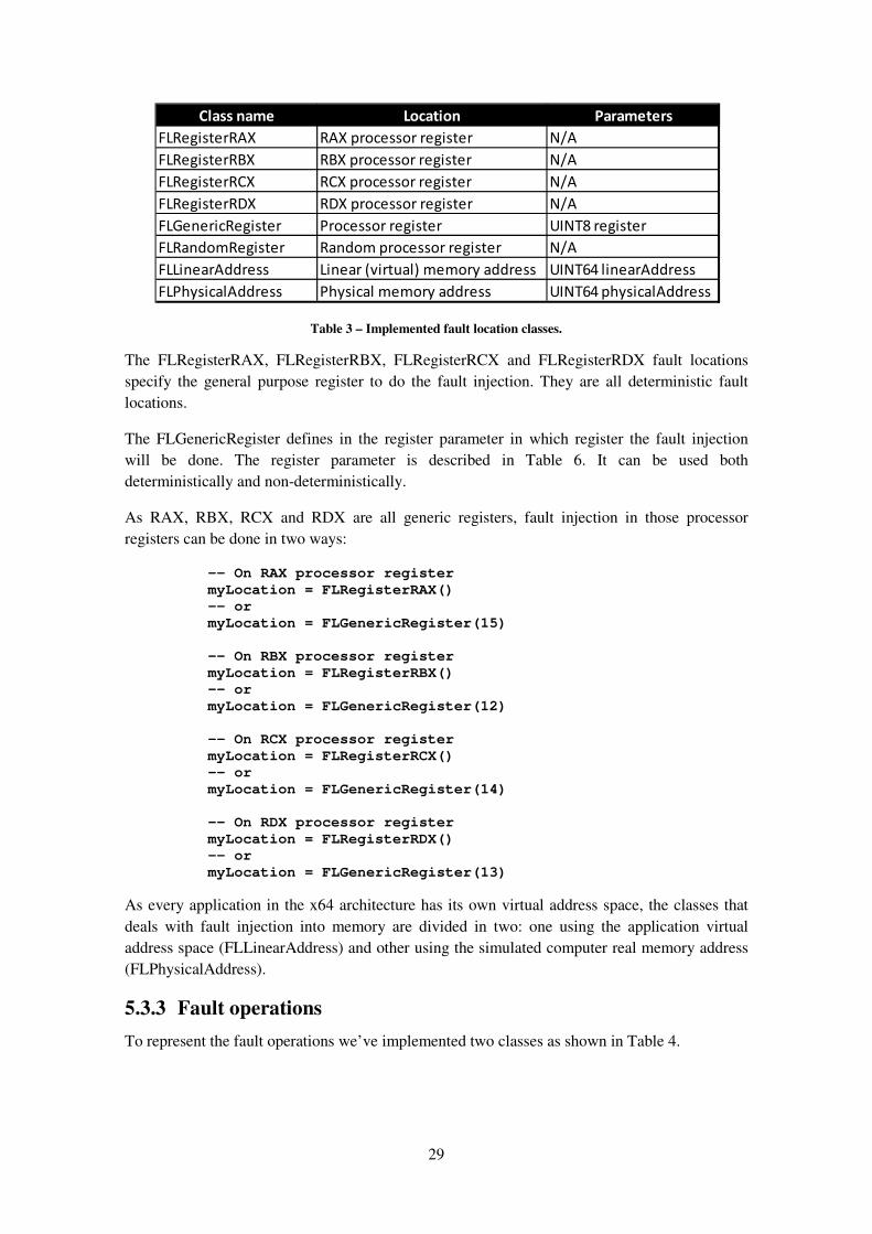
29
Table 3 – Implemented fault location classes.
The FLRegisterRAX, FLRegisterRBX, FLRegisterRCX and FLRegisterRDX fault locations
specify the general purpose register to do the fault injection. They are all deterministic fault
locations.
The FLGenericRegister defines in the register parameter in which register the fault injection
will be done. The register parameter is described in Table 6. It can be used both
deterministically and non-deterministically.
As RAX, RBX, RCX and RDX are all generic registers, fault injection in those processor
registers can be done in two ways:
-- On RAX processor register
myLocation = FLRegisterRAX()
-- or
myLocation = FLGenericRegister(15)
-- On RBX processor register
myLocation = FLRegisterRBX()
-- or
myLocation = FLGenericRegister(12)
-- On RCX processor register
myLocation = FLRegisterRCX()
-- or
myLocation = FLGenericRegister(14)
-- On RDX processor register
myLocation = FLRegisterRDX()
-- or
myLocation = FLGenericRegister(13)
As every application in the x64 architecture has its own virtual address space, the classes that
deals with fault injection into memory are divided in two: one using the application virtual
address space (FLLinearAddress) and other using the simulated computer real memory address
(FLPhysicalAddress).
5.3.3 Fault operations
To represent the fault operations we’ve implemented two classes as shown in Table 4.
Class name Location Parameters
FLRegisterRAX RAX processor register N/A
FLRegisterRBX RBX processor register N/A
FLRegisterRCX RCX processor register N/A
FLRegisterRDX RDX processor register N/A
FLGenericRegister Processor register UINT8 register
FLRandomRegister Random processor register N/A
FLLinearAddress Linear (virtual) memory address UINT64 linearAddress
FLPhysicalAddress Physical memory address UINT64 physicalAddress

30
Table 4 – Implemented fault operation classes.
The FOBitFlip operation inverts the state of the bit specified in the bitToFlip parameter. This
operation can be used deterministically or non-deterministically by assigning random values to
the bitToFlip parameter.
The FORandomBitFlip inverts the state of a randomly chosen bit. It can be used only for non-
deterministic fault injection purposes.
The FOAnd operation allows the use of two (or more) operations during a fault injection. It can
be used to generate a double (or multiple) bit change in the fault location or to generate more
than one fault injection in a single simulation by combining any bit flip operation with the
FOResetTrigger operation.
If it is desired to have multiple fault injections into a single simulation it could be done by using
the FOResetTrigger fault operation. Once operated, it increases an internal fault injection
counter (logging how many injections were made), and reset all fault triggers: the countdown
fault trigger loads its original value, the random countdown fault trigger randomly chooses other
counter and loads it and the timed based trigger starts counting a new timing based on the time
of the reset operation.
5.3.4 Using LUA
The framework was implemented in a way that the description of the fault injection is made
using the LUA programming language used in COTSon. There is no need of a distinct
configuration file or method to the simulation and the fault injection.
Figure 16 – A fault injection description using LUA.
Class name Operation Parameters
FOBitFlip Inversion of a specific bit state UINT8 bitToFlip
FORandomBitFlip Inversion of a random bit state N/A
FOAnd Do more than one operation FaultOperation operationA, FaultOperation operationB
FOResetTrigger Reset the fault trigger condition N/A
function faultinjection()
-- expcount is the experiment number informed to COSTon
expn = expcount - 1
addrRange = FTRIPInRange( 0x401260, 0x401346 )
trigger = FTRandomCountDown( 51660814, addrRange )
regToInject = expn % 16
location = FLGenericRegister( regToInject )
bitToFlip = (expn / 64)
operation = FOBitFlip(bitToFlip)
setFaultInjection(trigger, location, operation)
end
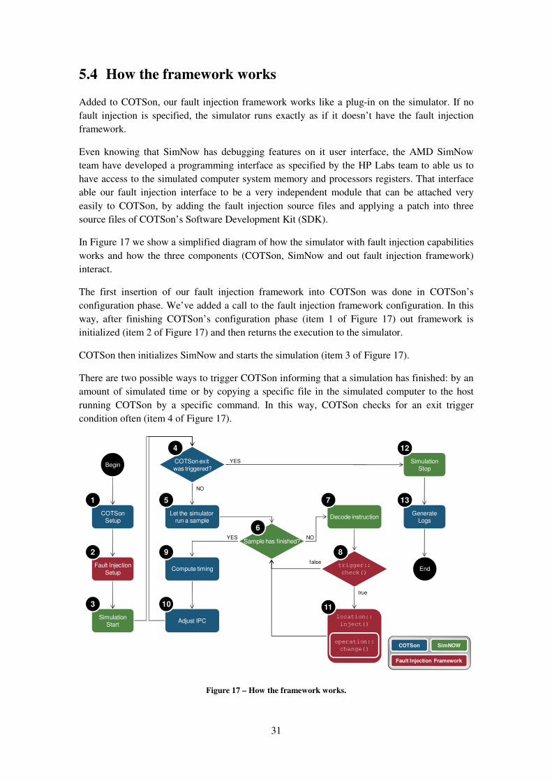
31
5.4 How the framework works
Added to COTSon, our fault injection framework works like a plug-in on the simulator. If no
fault injection is specified, the simulator runs exactly as if it doesn’t have the fault injection
framework.
Even knowing that SimNow has debugging features on it user interface, the AMD SimNow
team have developed a programming interface as specified by the HP Labs team to able us to
have access to the simulated computer system memory and processors registers. That interface
able our fault injection interface to be a very independent module that can be attached very
easily to COTSon, by adding the fault injection source files and applying a patch into three
source files of COTSon’s Software Development Kit (SDK).
In Figure 17 we show a simplified diagram of how the simulator with fault injection capabilities
works and how the three components (COTSon, SimNow and out fault injection framework)
interact.
The first insertion of our fault injection framework into COTSon was done in COTSon’s
configuration phase. We’ve added a call to the fault injection framework configuration. In this
way, after finishing COTSon’s configuration phase (item 1 of Figure 17) out framework is
initialized (item 2 of Figure 17) and then returns the execution to the simulator.
COTSon then initializes SimNow and starts the simulation (item 3 of Figure 17).
There are two possible ways to trigger COTSon informing that a simulation has finished: by an
amount of simulated time or by copying a specific file in the simulated computer to the host
running COTSon by a specific command. In this way, COTSon checks for an exit trigger
condition often (item 4 of Figure 17).
Figure 17 – How the framework works.
12
Begin
COTSonSetup
Fault Injection
Setup
SimulationStart
COTSon exit
was triggered?
Simulation
Stop
GenerateLogs
End
Let the simulator run a sample
Compute timing
Adjust IPC
Sample has finished?
Decode instruction
trigger::
check()
location::
inject()
operation::
change()
YES
NO
NO
false
true
YES
COTSon SimNOW
Fault Injection Framework
1
2
3
4
5
9
10
6
7
8
11
12
13
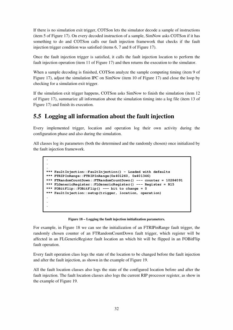
32
If there is no simulation exit trigger, COTSon lets the simulator decode a sample of instructions
(item 5 of Figure 17). On every decoded instruction of a sample, SimNow asks COTSon if it has
something to do and COTSon calls our fault injection framework that checks if the fault
injection trigger condition was satisfied (items 6, 7 and 8 of Figure 17).
Once the fault injection trigger is satisfied, it calls the fault injection location to perform the
fault injection operation (item 11 of Figure 17) and then returns the execution to the simulator.
When a sample decoding is finished, COTSon analyze the sample computing timing (item 9 of
Figure 17), adjust the simulation IPC on SimNow (item 10 of Figure 17) and close the loop by
checking for a simulation exit trigger.
If the simulation exit trigger happens, COTSon asks SimNow to finish the simulation (item 12
of Figure 17), summarize all information about the simulation timing into a log file (item 13 of
Figure 17) and finish its execution.
5.5 Logging all information about the fault injection
Every implemented trigger, location and operation log their own activity during the
configuration phase and also during the simulation.
All classes log its parameters (both the determined and the randomly chosen) once initialized by
the fault injection framework.
Figure 18 – Logging the fault injection initialization parameters.
For example, in Figure 18 we can see the initialization of an FTRIPinRange fault trigger, the
randomly chosen counter of an FTRandomCountDown fault trigger, which register will be
affected in an FLGenericRegister fault location an which bit will be flipped in an FOBitFlip
fault operation.
Every fault operation class logs the state of the location to be changed before the fault injection
and after the fault injection, as shown in the example of Figure 19.
All the fault location classes also logs the state of the configured location before and after the
fault injection. The fault location classes also logs the current RIP processor register, as show in
the example of Figure 19.
.
.
.
*** FaultInjection::FaultInjection() - Loaded with defaults
*** FTRIPInRange::FTRIPInRange(0x401260, 0x401346)
*** FTRandomCountDown::FTRandomCountDown() --- counter = 10284091
*** FLGenericRegister::FLGenericRegister() --- Register = R15
*** FOBitFlip::FOBitFlip() --- bit to change = 0
*** FaultInjection::setup(trigger, location, operation)
.
.
.

33
Figure 19 – Operation and location standard logging.
We have also developed two auxiliary classes with debugging purposes, as shown in Table 5.
These two auxiliary debugging classes can be associated to any fault trigger. When associated to
a fault trigger, those classes will provide additional information once the fault trigger class gets
a trigger state.
Table 5 – Implemented debugging classes.
The FDDumpRegisters debugging class dumps all x64 general purpose processor registers and
also some additional processor states that can be useful for evaluation of the state of the
application during the fault injection, as shown in Figure 20.
Figure 20 – Dump of processor registers and state.
In a deterministic approach, FDDumpRegisters can be used to ensure the desired fault injection
trigger (when to do the injection) by verifying all processor registers as a finger-print of the fault
trigger. In a non-deterministic approach, FDDumpRegisters can be used create a deterministic
condition capable of reproduce the non-deterministic fault injection configuration.
.
.
.
*** FaultInjection::check() --- injecting...
*** FLGenericRegister::inject()
*** FLGenericRegister::inject() --- cpuid = 0 ; RegisterRIP = 4012f6
*** FLGenericRegister::notice() --- Change in cpuid = 0 ; register R15 = 0
*** FOBitFlip::change() --- Changing bit #0 ... Original UINT64: 0 Changed UINT64: 1
*** FLGenericRegister::notice() --- Change in cpuid = 0 ; register R15 = 1
.
.
.
Class name Debug
FDDumpRegisters Dump all processor registers
FDDumpInstruction Dump the current RIP register and the assembly instruction pointed by the RIP
.
.
.
*** FLGenericRegister::inject() --- RegisterRIP:401594
*** FLGenericRegister::notice() --- Change in R14 = 0
*** FDDumpRegisters::dump() --- CurrentPL = 3, EFERRegister = d01, MachineState = 0, Revision = 30064,
SMMBase = a0000, CR4 = 6e0, CR3 = cd9a000, CR0 = 80050033, DR7 = 400, DR6 = ffff0ff0, EFLAGS = 216,
RIP = 401594, R15 = 0, R14 = 0, R13 = 7fffffbd6ba0, R12 = 401bb0, R11 = 2aaaaad74860, R10 = 0, R9 = 68ca8,
R8 = 6027a0, RDI = 0, RSI = 80, RBP = 7fffffbd6630, RSP = 7fffffbd6600, RBX = 0, RDX = 622a60, RCX = 0,
RAX = 13f60
*** FORandomBitFlip::getBitTiFlip() --- bit to flip = 29
*** FORandomBitFlip::change() --- Changing bit #29... Original UINT40: 0 Changed UINT40: 20000000000
*** FLGenericRegister::notice() --- Change in R14 = 20000000000
.
.
.

34

35
Chapter 6 Experimental evaluation
6.1 Introduction
To achieve the objectives of this master thesis we made three experimental evaluations using the
fault injection environment developed.
Each simulation with fault injection generates four log files that we use to analyze what
happened after the fault injection:
a) COTSon output log: have all information about the simulation, amount of instructions
simulated, memory hierarchy counters, simulated computer components and timing
information;
b) Application output: have the result of the execution of the application;
c) Simulated operating system log: have information about what kind of exception the
fault injected application may generate;
d) Fault injection framework log: have all information about the fault injection
configuration that was executed (when the injection was made, where the injection was
made and what operation was used). This log has also the processor registers state just
before and after the fault injection.
By analyzing these logs we can classify a simulation with fault injection in five different ways,
as show in Figure 21.
Figure 21 – Possible results of a simulation with fault injection.
In a correct experiment simulation with a fault injection the application runs normally, finishes
properly and the result provided by the application is the same as if the execution of the
application didn’t have fault injections. This situation of a correct result even doing a fault
injection is represented in Figure 6 (outcomes of a transient fault) by the items 2 (the bit
changed was never read by the application) and 6 (bit has been read but didn’t affected the
application outcome).
The application was executed until it’s end, finished properly and provided the correct result.
The application was executed, finished properly and provided
an incorrect result.
The machine/operating system detected an invalid operation
of the application. The application didn’t finished properly.
The simulation finished by a TIMEOUT trigger instead of by the
generation of the experiment result file.
The application’s fault detection mechanism was triggered.
Correct
Incorrect
System Detected
Timeout
Fault Detected

36
In an incorrect experiment simulation with a fault injection the application runs normally,
finishes properly and generates a result, but the result generated is different of the result
provided by the application is the same as if the execution of the application didn’t have fault
injections. This situation of incorrect result is represented in Figure 6 by the item 7 (SDC),
representing an unnoticed data corruption.
In a system detected experiment simulation with a fault injection the application runs normally
but didn’t finishes properly and also didn’t generate any result. Interrupted by the operating
system or by the simulated computer processor, the application didn’t achieve its objective, but
the running environment knows that something wrong happened. This situation of a system
detection of a transient fault is represented in Figure 6 by the items 4 (False DUE) and 5 (True
DUE), both representing a detected unrecoverable error.
As every simulation may have a configured limit of simulated execution time, if the simulation
keeps running until reach the configured limit because the application is still running, the
simulator will stop the simulation and this experiment will be classified as a timeout. This
situation of a timeout is represented in Figure 6 by the item 7 (SDC). A timeout condition is a
particular case of a silent data corruption. In this case, the silent data corruption affected
something in the application that makes the application run for more than the expected amount
of time.
If the tested application has some fault detection mechanism, the experiment may be classified
as fault detected if the application generates some information about a detected fault (or error).
This situation of a fault detected by application is represented in Figure 6 by the items 4 (False
DUE) and 5 (True DUE), both representing a detected unrecoverable error.
All simulations used in this work used the same simulated machine with a single core AMD
Opteron Processor 246 (Family 15, Model 5, Stepping 10) running at 2.2Ghz, with 512MB of
RAM, 16KB of instruction cache, 16KB of data cache and 512KB of L2 cache.
As explained previously in Chapter 4, SimNow as a functional simulator don’t deal with timing
and doesn’t have information about the simulated computer memory hierarchy. In this way,
Figure 22 has an overview of the simulated computer interconnection architecture in SimNow
and Figure 23 has the memory hierarchy of the simulated computer in COTSon.
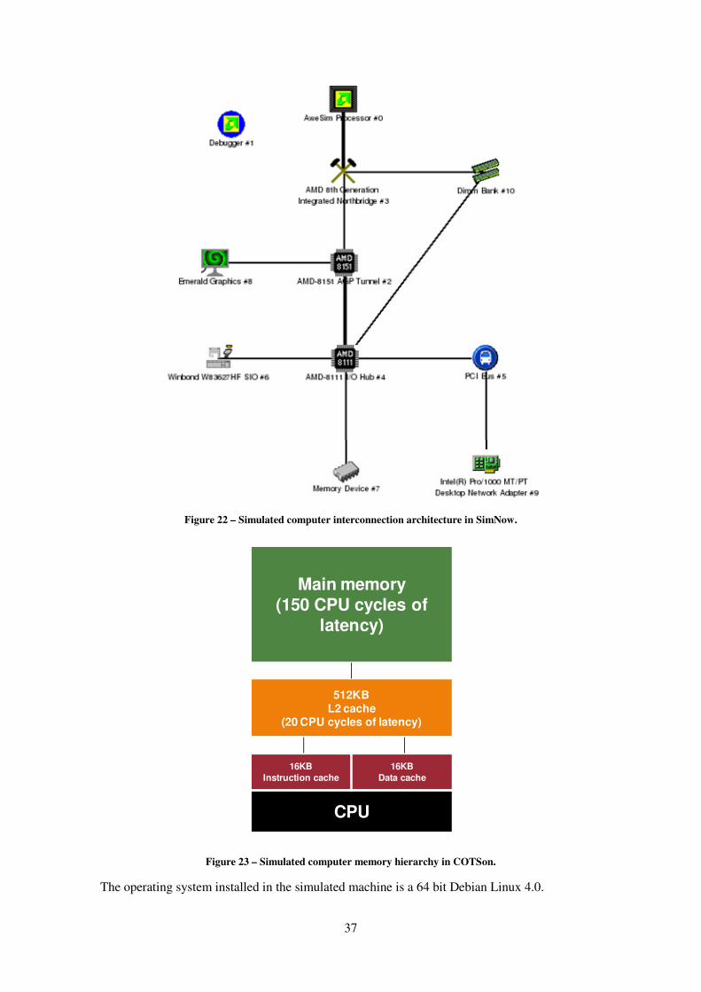
37
Figure 22 – Simulated computer interconnection architecture in SimNow.
Figure 23 – Simulated computer memory hierarchy in COTSon.
The operating system installed in the simulated machine is a 64 bit Debian Linux 4.0.
512KBL2 cache
(20 CPU cycles of latency)
CPU
16KB
Instruction cache
16KB
Data cache
Main memory
(150 CPU cycles of
latency)
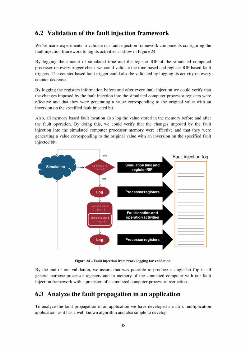
38
6.2 Validation of the fault injection framework
We’ve made experiments to validate our fault injection framework components configuring the
fault injection framework to log its activities as show in Figure 24.
By logging the amount of simulated time and the register RIP of the simulated computed
processor on every trigger check we could validate the time based and register RIP based fault
triggers. The counter based fault trigger could also be validated by logging its activity on every
counter decrease.
By logging the registers information before and after every fault injection we could verify that
the changes imposed by the fault injection into the simulated computer processor registers were
effective and that they were generating a value corresponding to the original value with an
inversion on the specified fault injected bit.
Also, all memory based fault location also log the value stored in the memory before and after
the fault operation. By doing this, we could verify that the changes imposed by the fault
injection into the simulated computer processor memory were effective and that they were
generating a value corresponding to the original value with an inversion on the specified fault
injected bit.
Figure 24 – Fault injection framework logging for validation.
By the end of our validation, we assure that was possible to produce a single bit flip in all
general purpose processor registers and in memory of the simulated computer with our fault
injection framework with a precision of a simulated computer processor instruction.
6.3 Analyze the fault propagation in an application
To analyze the fault propagation in an application we have developed a matrix multiplication
application, as it has a well known algorithm and also simple to develop.
trigger::
check()
location::
inject()
operation::
change()
true
__________________________________
_________________
_________________
_________________
__________________________________
_________________
_________________
_________________
__________________________________
_________________
_________________
_________________
__________________________________
_________________
_________________
_________________
__________________________________
_________________
_________________
_________________
Simulation
false
Simulation time and
register RIP
Fault injection log
Processor registers
Processor registers
Log
Log
Fault location and
operation activities
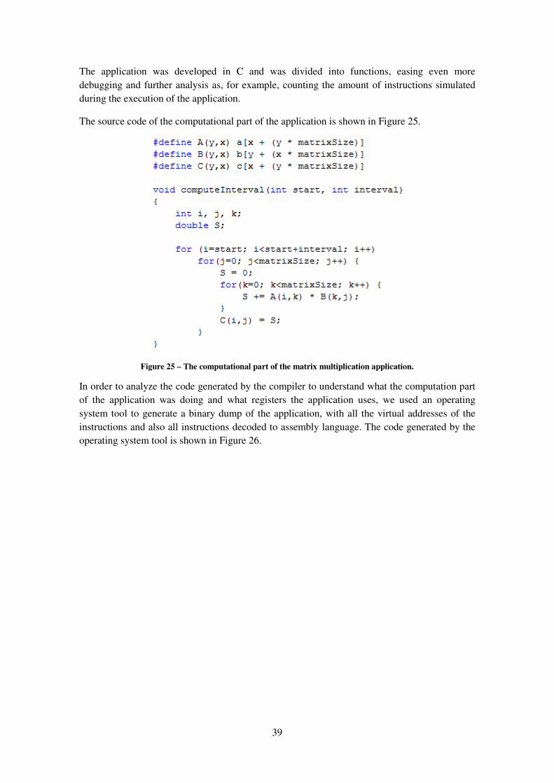
39
The application was developed in C and was divided into functions, easing even more
debugging and further analysis as, for example, counting the amount of instructions simulated
during the execution of the application.
The source code of the computational part of the application is shown in Figure 25.
Figure 25 – The computational part of the matrix multiplication application.
In order to analyze the code generated by the compiler to understand what the computation part
of the application was doing and what registers the application uses, we used an operating
system tool to generate a binary dump of the application, with all the virtual addresses of the
instructions and also all instructions decoded to assembly language. The code generated by the
operating system tool is shown in Figure 26.

40
Figure 26 – Assembly dump of the computational part of the application
6.3.1 Generating correct result
By analyzing the assembly dump of the computational part of the application Figure 26, we
noticed that the RAX general purpose register had its value over written in the instruction of the
address 0x4012ed and the last used of its previous value was in instruction 0x4012d3. In this
way, any change made in the RAX general purpose register after the instruction in address
0x4012d3 and before the instruction in address 0x4012ed will produce a latent error that never
will be noticed.

41
We have made 60 (ten per trigger address) simulated fault injection experiments using the RAX
general purpose register as fault location and random bit flip as fault operation but triggering the
fault injection between the addresses 0x4012d7 and 0x4012ed.
In all 60 injections we could attest the change in the randomly chosen bit by the simulation logs.
Also, all 64 simulations were classified as correct.
6.3.2 Generating system detected condition and incorrect result
By analyzing the assembly dump of the computational part of the application Figure 26, we
noticed that the RAX general purpose register was used in addresses 0x4012b1 and 0x4012d3
as a pointer to a data memory region. In this way, some changes made in the RAX general
purpose register in these addresses may produce a memory access violation for changes on
higher valued bits.
We have made 20 (ten per trigger address) fault injection experiments using the RAX general
purpose register as fault location and random bit flip as fault operation but triggering the fault
injection in the address 0x4012b1 or in the address 0x4012d3.
Those simulated fault injections that changed a bit higher than or equal 20 (it was 14
simulations) have generated a system detected DUE. The six simulations that changed the RAX
register in a bit less than 20 have generated five SDC (the RAX register pointed to a memory
address still valid to the application but with a different content) and one correct simulation as
in this case the RAX register pointed to a memory address still valid to the application and with
a content equal to the previously pointed one.
6.3.3 Experiment conclusions
Analyzing a well known application, with access to its source code and binary file it is possible
to understand how the application deals with the simulated computer.
In this way, it is possible to create very specific scenarios with well elaborated fault injection
strategies to generate the many different outcomes. As more knowledge about the application
we have, more we can refine our fault injection strategy saving time by reducing the amount of
experiments needed to obtain a desired condition.
6.4 Analyze an application robustness
To analyze an application robustness against transient faults in processor registers, we used the
same matrix multiplication application used in the previous experiment to do a fault injection
campaign using non-deterministic fault injection strategy.
Also, to enhance the analysis, we have compiled the application with and without compiler
optimizations and executed the simulations using the two compiled versions of the application.
As commonly strategies used to enhance the performance of applications tends to lower the
application robustness against faults, we wanted to analyze if improving application
performance by optimizing its compilation turns the application binary code also lowers the
application robustness against transient faults.

42
6.4.1 Experiment setup
We used two fault injection campaigns in this experiment: one with the non-optimized version
of the matrix multiplication application and other with the optimized one.
For each fault injection campaign, the fault injection was configured to inject the fault only
during the execution of the function that actually computes the multiplication. To do this, have
generated a dump of the binary code of each version of the application and looked for the
addresses of the function to program the fault trigger.
The fault trigger was also programmed to do the fault injection after a randomly chosen amount
of processor instructions simulated. To determine the range of this randomly chosen value, we
have counted the amount of instructions simulated in a simulation without fault injection.
Table 6 – X64 general purpose integer registers.
As we wanted to analyze the effect on every general purpose register of the simulated processor,
the fault location vary in a range from 0 to 15 as according with the target register as shown in
Table 6. The volatility of a register show in the table implies in that if a function intends to use
the register it show save the register original value and restore this value before finishing
computing.
As the simulated machine and the operating system installed are both 64 bit, the fault injection
campaign injected faults into each one of the 64 bits of each register.
409664164TriggersOperationsLocationsnsSilmulatio
64bits) 64each in flip(bit Operations
16)(registers Locations
4 simulated) nsinstructio ofamount (randomly Triggers
=××=××=
=
=
=
Equation 4 – Amount of simulations per application compiled version.
As shown in Equation 4, for each version of the compiled application we intended to do 4096
simulations. The total amount of simulations to do this experiment was 8192.
Index Register Volatile Purpose
0 R15 No Must be preserved by called function
1 R14 No Must be preserved by called function
2 R13 No Must be preserved by called function
3 R12 No Must be preserved by called function
4 R11 Yes Used in syscall/sysret instructions
5 R10 Yes Used in syscall/sysret instructions
6 R9 Yes Fourth integer argument
7 R8 Yes Third integer argument
8 RDI No Must be preserved by called function
9 RSI No Must be preserved by called function
10 RBP No Can be used as a frame pointer and must be preserved by called function.
11 RSP No Stack Pointer
12 RBX No Must be preserved by called function
13 RDX Yes Second integer argument
14 RCX Yes First integer argument
15 RAX Yes Return value register

43
6.4.2 Experiment results
After executing all simulations of this experiment, for each compiled version of the application
there was a directory tree with all simulations logs.
A script was developed to summarize all general information contained on the logs and generate
a comma separated value file that is imported to a Microsoft Excel template worksheet that
generates three charts:
a) Fault injection simulation outcomes;
b) Per registers simulation outcomes;
c) Per nibble simulation outcomes.
The results of the two versions of the application were very different. The optimized version of
the application had less than half of correct results of the non-optimized one, as shown in Figure
27. Also, the amount of incorrect (SDC) results of the optimized version was more than 16
times the amount of incorrect results of the non-optimized version. The amount of system detect
results of the optimized version was more than four times the amount of system detected results
of the experiments with the non-optimized version of the application.
By analyzing the information in Figure 28 we can notice that the non-optimized version is only
affected by changes in three processor registers: RBP, RDX and RAX. The optimized version of
the application had more registers that once changed by the fault injection produced results
others than correct. The experiments of the optimized version were not affected only by changes
in R15 and R14 processor registers.
The information in Figure 29 shows that in both experiments there were incorrect results only
when the operation of the fault injection was a flip on a bit lower than 32. By analyzing the
assembly code of the applications we noticed that in many cases the processor registers are used
as pointers to memory regions in instruction that only uses the less significant 32 bits of the
processor registers.
We could also notice in Figure 29 that as greater is the bit operated by the fault injection, the
amount of incorrect result lows and the amount of system detected results rises. By analyzing
this situation we noticed that as some registers are used as pointers to memory regions, the
changes in less significant bits of the registers made that registers still pointing to valid memory
regions to the tested application. This let the application read an undesired value on it operations
producing incorrect experiment results (SDC). On the other hand, the changes in more
significant bits of the registers made that registers pointing to invalid memory regions to the
tested application. Once trying to access these invalid memory regions, instead of obtaining an
undesired value, the protection mechanism of the processor architecture triggered to the
operating system an access violation. The operating system then aborted the application
execution producing a system detected result to the experiment.

44
Without compiler optimization With compiler optimization
Figure 27 – Fault injection simulation outcomes.
Without compiler optimization With compiler optimization
Figure 28 – Per register simulation outcomes.
Without compiler optimization With compiler optimization
Figure 29 – Per nibble simulation outcomes.
6.4.3 Experiment conclusions
Compiler optimized applications are less robust against transient faults as more registers are
used due to compiler optimization.
89,18%
1,44%
9,28%
0,10%
33,59%
23,68%
39,79%
2,93%
Correct App DetectedSys Detected TimeoutIncorrect
4
245
88
47
29
30
256 256 256 256 256 256 256 256 256 256
7
256 256
139
256
179
0%
10%
20%
30%
40%
50%
60%
70%
80%
90%
100%
R15 R14 R13 R12 R11 R10 R9 R8 RDI RSI RBP RSP RBX RDX RCX RAX
72
43
1 4
162 164
4
36
164
184166 164
256
4
163 163
90
8
92
110
49
39
71
64
91
108120
64 64
256 256
4
176
142128
53
261
144132
29 29
0%
10%
20%
30%
40%
50%
60%
70%
80%
90%
100%
R15 R14 R13 R12 R11 R10 R9 R8 RDI RSI RBP RSP RBX RDX RCX RAX
Correct App DetectedSys Detected TimeoutIncorrect
416 15 12 16 18 25 27 33 30 27 32 27 25 27 27 23
167 3 6
1410 3
224234 237 234
224 221 226 223 226 229 224 229 231 229 229 233
0%
10%
20%
30%
40%
50%
60%
70%
80%
90%
100%
0-3 4-7 8-11 12-15 16-19 20-23 24-27 28-31 32-35 36-39 40-43 44-47 48-51 52-55 56-59 60-63
1 3
28 32 24 16 1616 16 16
2027
95
132
164
143 143 143 144 142 144 142 143
163150 151
132
153
102
75
44
7690 86
76
4435 33 32
113 113 113 112 114 112 114 113
0%
10%
20%
30%
40%
50%
60%
70%
80%
90%
100%
0-3 4-7 8-11 12-15 16-19 20-23 24-27 28-31 32-35 36-39 40-43 44-47 48-51 52-55 56-59 60-63
Correct App DetectedSys Detected TimeoutIncorrect

45
It is important to have strict memory allocation as some registers are used as pointers and
reserving more memory than the application needs may let changes in register point to valid
memory addresses after a transient fault.
6.5 Test fault detection mechanisms
To verify if a fault detection mechanism detects the faults injected with our fault injection
framework, we changed the matrix multiplication application source code using two of the three
purely software based mechanism to hardening applications against transient faults [22]:
duplicating the intermediate computations and verifying twice the conditional control
instructions.
Figure 30 – Duplication of the intermediate computation.
With the objective of preventing the use of a faulty variable, the authors of [22] suggest that all
intermediary computation should be doubled and verified as described in Figure 30.
Also, with the same strategy of doubling computation to ensure fault detection, the authors of
[22] suggest that every time that a condition is verified, it should be checked again in order to
prevent that a faulty condition be used during the application execution. The method used for
verify twice the conditional instructions is described in Figure 31.
Figure 31 – Double verification of the conditional instructions.
The Figure 32 shows the previously showed computational part of the matrix multiplication
application changed to detect faults using the previously mentioned detection mechanisms.
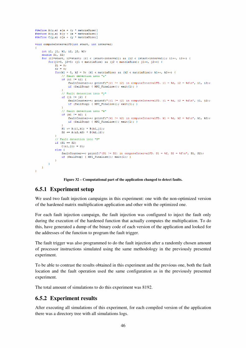
46
Figure 32 – Computational part of the application changed to detect faults.
6.5.1 Experiment setup
We used two fault injection campaigns in this experiment: one with the non-optimized version
of the hardened matrix multiplication application and other with the optimized one.
For each fault injection campaign, the fault injection was configured to inject the fault only
during the execution of the hardened function that actually computes the multiplication. To do
this, have generated a dump of the binary code of each version of the application and looked for
the addresses of the function to program the fault trigger.
The fault trigger was also programmed to do the fault injection after a randomly chosen amount
of processor instructions simulated using the same methodology in the previously presented
experiment.
To be able to contrast the results obtained in this experiment and the previous one, both the fault
location and the fault operation used the same configuration as in the previously presented
experiment.
The total amount of simulations to do this experiment was 8192.
6.5.2 Experiment results
After executing all simulations of this experiment, for each compiled version of the application
there was a directory tree with all simulations logs.

47
The same script developed to the previously presented experiment was used to summarize all
general information contained on the logs and generate a comma separated value file that was
imported to a Microsoft Excel template worksheet to generate the charts.
6.5.2.1 Comparing without and with the fault detection mechanism
In this comparison, we used the results of the non-optimized version of the application without
the fault detection mechanism obtained in the previously presented experiment and the non-
optimized version of the application with the fault detection mechanism.
The first difference noticed between the results obtained with the experiments without fault
detection and with fault detection, shown in Figure 34, is that in the second one we had
application detected results.
The second difference is that in the experiment with fault detection we had almost no SDC
results (only one).
Figure 33 – Assembly code of the region where the SDC was produced.
This one SDC produced was result of a fault injected happened with a fault injected into the
register RAX location, operating a flip in the bit 31, just after the simulator had simulated the
instruction pointed by register RIP in address 0x401527.
Analyzing the assembly code of the region where the fault was injected shown in Figure 33 we
noticed that the fault was injected just after a comparison for fault detection in the register RAX
and just before an attribution using the verified value. As presented in [22], we already knew
that using the fault detection mechanism selected for in this experiment could produce some
SDC cases if the fault occurs just after the test for fault detection and just before the used of the
tested value.
In Figure 35 and in Figure 36 is possible to observe the almost substitution of the incorrect
results in the experiment without fault detection mechanism by the application detected results
in the experiment with fault detection mechanism.

48
Without fault detection mechanism With fault detection mechanism
Figure 34 – Fault injection simulation outcomes.
Without fault detection mechanism With fault detection mechanism
Figure 35 – Per register simulation outcomes.
Without fault detection mechanism With fault detection mechanism
Figure 36 – Per nibble simulation outcomes.
6.5.2.2 Comparing without and with compiler optimization
In this comparison, we used the results of the non-optimized and the optimized versions of the
application with the fault detection mechanism.
As observed in the experiment described previously in session 6.4, the optimized version of the
application was more affected to the faults injected than the non-optimized one. But, in this
89,18%
1,44%
9,28%
0,10%
89,97%
0,02%
7,76%
0,15%2,10%
Correct App DetectedSys Detected TimeoutIncorrect
4
245
88
47
29
30
256 256 256 256 256 256 256 256 256 256
7
256 256
139
256
179
0%
10%
20%
30%
40%
50%
60%
70%
80%
90%
100%
R15 R14 R13 R12 R11 R10 R9 R8 RDI RSI RBP RSP RBX RDX RCX RAX
4023 23
6
210
67
41
1
256 256 256 256 256 256 256 256 256 256 256 256
166
256
191
0%
10%
20%
30%
40%
50%
60%
70%
80%
90%
100%
R15 R14 R13 R12 R11 R10 R9 R8 RDI RSI RBP RSP RBX RDX RCX RAX
Correct App DetectedSys Detected TimeoutIncorrect
416 15 12 16 18 25 27 33 30 27 32 27 25 27 27 23
167 3 6
1410 3
224234 237 234
224 221 226 223 226 229 224 229 231 229 229 233
0%
10%
20%
30%
40%
50%
60%
70%
80%
90%
100%
0-3 4-7 8-11 12-15 16-19 20-23 24-27 28-31 32-35 36-39 40-43 44-47 48-51 52-55 56-59 60-63
17 21 14 9 165 3 1
65
1 6 1015
21 31 31 25 23 20 26 27 26 26 25
1
228 234 236 237225 230 222 223 231 233 236 230 229 230 230 231
0%
10%
20%
30%
40%
50%
60%
70%
80%
90%
100%
0-3 4-7 8-11 12-15 16-19 20-23 24-27 28-31 32-35 36-39 40-43 44-47 48-51 52-55 56-59 60-63
Correct App DetectedSys Detected TimeoutIncorrect

49
case, the difference was less significant than in the comparison of the applications without fault
detection mechanism.
By analyzing the information in Figure 38 we can notice that the non-optimized version is only
affected by changes in three processor registers: RBP, RDX and RAX. The optimized version of
the application had more registers that once changed by the fault injection produced results
others than correct. The experiments of the optimized version were not affected only by changes
in R15, R14, R13 and R11 processor registers.
In the Figure 37 we noticed that the optimized version of the application had no application
detected results and presented more than 13% of the results as incorrect. By analyzing the logs
of the fault injection campaign and the assembly code of the application with fault detection
mechanism and compiled with optimizations we noticed that the compiler has changed the order
of the instructions in a way that didn’t change the application results in a faultless execution, but
may change in presence of faults. Also, the compiler has removed the code that it assumed to be
unnecessary to obtain the desired result in a faultless execution.
By doing the optimization in the hardened version of the application, the compiler almost
removed the fault detection mechanism of the compiled application by assuming the redundant
execution an expensive unnecessary code
Also, as in session 6.4, we could notice in Figure 39 that as greater is the bit operated by the
fault injection, the amount of incorrect result lows and the amount of system detected results
rises. This is the same situation we noticed previously that as some registers are used as pointers
to memory regions.
Without compiler optimization With compiler optimization
Figure 37 – Fault injection simulation outcomes.
89,97%
0,02%
7,76%
0,15%2,10%
61,87%
13,65%
22,73%
1,76%
Correct App DetectedSys Detected TimeoutIncorrect
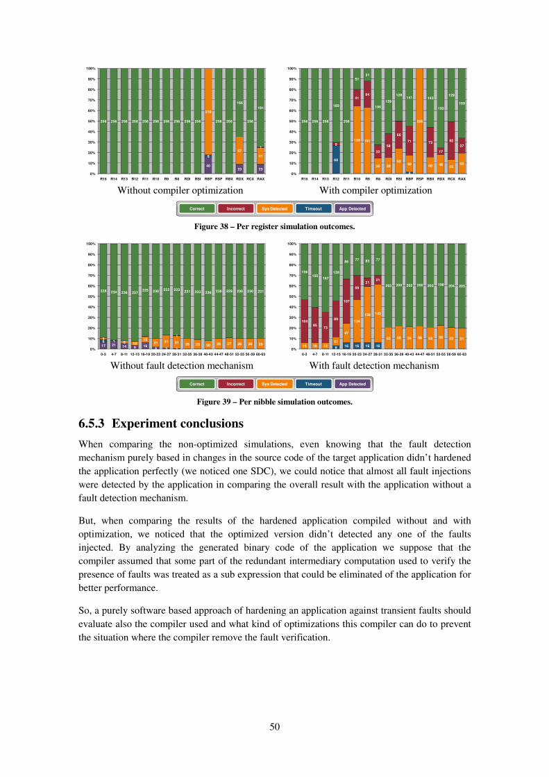
50
Without compiler optimization With compiler optimization
Figure 38 – Per register simulation outcomes.
Without fault detection mechanism With fault detection mechanism
Figure 39 – Per nibble simulation outcomes.
6.5.3 Experiment conclusions
When comparing the non-optimized simulations, even knowing that the fault detection
mechanism purely based in changes in the source code of the target application didn’t hardened
the application perfectly (we noticed one SDC), we could notice that almost all fault injections
were detected by the application in comparing the overall result with the application without a
fault detection mechanism.
But, when comparing the results of the hardened application compiled without and with
optimization, we noticed that the optimized version didn’t detected any one of the faults
injected. By analyzing the generated binary code of the application we suppose that the
compiler assumed that some part of the redundant intermediary computation used to verify the
presence of faults was treated as a sub expression that could be eliminated of the application for
better performance.
So, a purely software based approach of hardening an application against transient faults should
evaluate also the compiler used and what kind of optimizations this compiler can do to prevent
the situation where the compiler remove the fault verification.
4023 23
6
210
67
41
1
256 256 256 256 256 256 256 256 256 256 256 256
166
256
191
0%
10%
20%
30%
40%
50%
60%
70%
80%
90%
100%
R15 R14 R13 R12 R11 R10 R9 R8 RDI RSI RBP RSP RBX RDX RCX RAX
68
4
164 161
38 39
6240
256
40 4635
50
8
4164
32
58
66
71 73
17
92
37
256 256 256
180
256
5131
186
159
128141 143
193
129
169
0%
10%
20%
30%
40%
50%
60%
70%
80%
90%
100%
R15 R14 R13 R12 R11 R10 R9 R8 RDI RSI RBP RSP RBX RDX RCX RAX
Correct App DetectedSys Detected TimeoutIncorrect
17 21 14 9 165 3 1
65
1 6 1015
21 31 31 25 23 20 26 27 26 26 25
1
228 234 236 237225 230 222 223 231 233 236 230 229 230 230 231
0%
10%
20%
30%
40%
50%
60%
70%
80%
90%
100%
0-3 4-7 8-11 12-15 16-19 20-23 24-27 28-31 32-35 36-39 40-43 44-47 48-51 52-55 56-59 60-63
8 16 16 16 1616 16 16
21
47
104
136 142
53 56 54 56 53 58 52 51
10485
73
89
107
59
2121
136155
167
138
8677 83 77
203 200 202 200 203 198 204 205
0%
10%
20%
30%
40%
50%
60%
70%
80%
90%
100%
0-3 4-7 8-11 12-15 16-19 20-23 24-27 28-31 32-35 36-39 40-43 44-47 48-51 52-55 56-59 60-63
Correct App DetectedSys Detected TimeoutIncorrect
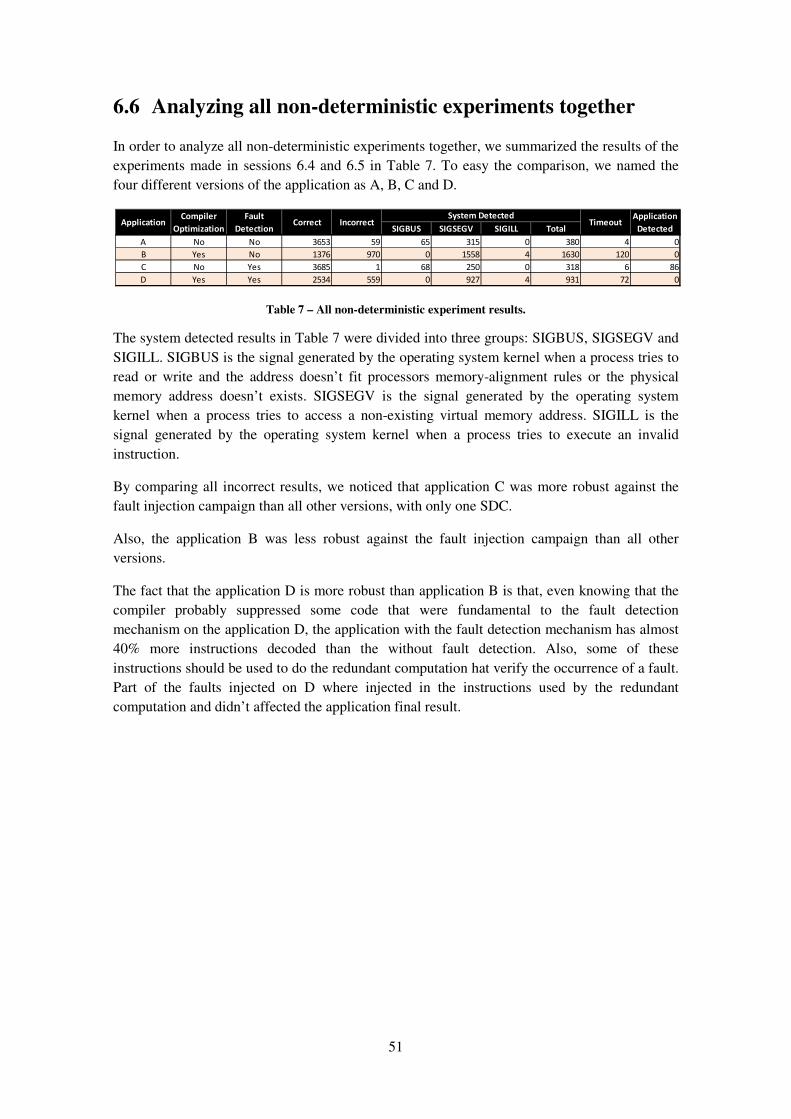
51
6.6 Analyzing all non-deterministic experiments together
In order to analyze all non-deterministic experiments together, we summarized the results of the
experiments made in sessions 6.4 and 6.5 in Table 7. To easy the comparison, we named the
four different versions of the application as A, B, C and D.
Table 7 – All non-deterministic experiment results.
The system detected results in Table 7 were divided into three groups: SIGBUS, SIGSEGV and
SIGILL. SIGBUS is the signal generated by the operating system kernel when a process tries to
read or write and the address doesn’t fit processors memory-alignment rules or the physical
memory address doesn’t exists. SIGSEGV is the signal generated by the operating system
kernel when a process tries to access a non-existing virtual memory address. SIGILL is the
signal generated by the operating system kernel when a process tries to execute an invalid
instruction.
By comparing all incorrect results, we noticed that application C was more robust against the
fault injection campaign than all other versions, with only one SDC.
Also, the application B was less robust against the fault injection campaign than all other
versions.
The fact that the application D is more robust than application B is that, even knowing that the
compiler probably suppressed some code that were fundamental to the fault detection
mechanism on the application D, the application with the fault detection mechanism has almost
40% more instructions decoded than the without fault detection. Also, some of these
instructions should be used to do the redundant computation hat verify the occurrence of a fault.
Part of the faults injected on D where injected in the instructions used by the redundant
computation and didn’t affected the application final result.
SIGBUS SIGSEGV SIGILL Total
A No No 3653 59 65 315 0 380 4 0
B Yes No 1376 970 0 1558 4 1630 120 0
C No Yes 3685 1 68 250 0 318 6 86
D Yes Yes 2534 559 0 927 4 931 72 0
ApplicationFault
Detection
Compiler
Optimization
System DetectedCorrect Incorrect Timeout
Application
Detected

52

53
Chapter 7 Conclusion and future work
7.1 Conclusion
With the evolution of computer processors for better performance, the computer chips are
becoming less robust against transient faults because of its size reduction and higher density of
components operating at lower voltages.
This reduction is computer chips robustness is evidencing the occurrence of transient fault and
their biggest risk: dealing with transient faults in computer processors that generates undetected
data corruption changing the final result of an application without noticing.
The risk of having an execution affected by a transient fault when running an application in a
high performance computer system is greater than running an application using a single
computer chip as the risk of having an execution affected by a transient fault in high
performance computers is multiplied by the amount of computer processors working together.
Since transient faults occur in a very unpredictable way, as purposed in the beginning of this
work, we now have an environment with fault injection capabilities able to help us to study the
effects of these faults in computers, operating systems and applications.
Our environment uses a full system simulator and allows both deterministic and non-
deterministic fault injections campaigns and generates enough information about the fault
injection to help in the further analysis necessary to a better understanding of the effects of a
transient fault.
By selecting a full system simulator as environment to inject faults we also could achieve both
precision and accuracy by having full control of the simulated computer processor.
Also, we can assume that our fault injection environment produce almost no impact into the
tested application. The fault injection mechanism isn’t simulated with the tested application or
operating system because it operates in a lower level of abstraction and the timing of the
simulated computer is manipulated by the simulator.
With our fault injection environment we achieve a very transparent fault injection environment,
as for dealing with fault injection isn’t necessary changes into the simulated computer operating
system or in the tested application.
Our environment uses a programming language to describe how to reproduce a transient fault
by informing when to reproduce the fault, where the fault will affect the simulated computer and
what to the produced fault will change.
With the environment developed, we were able to evaluate the effects of single bit flip transient
faults on processor registers into an application, analyze an application robustness against single
bit flip transient faults on processor registers and test a fault detection mechanism.

54
7.2 Future work
As future work, as COTSon allows the simulation of computer clusters, it should be interesting
to extend our fault injection framework to allow clustered coordinated fault injection
campaigns, where the trigger could be determined by a determined group of cluster nodes
conditions.
Also, as transient faults could lead to data corruption, it is very important to study fault
detection mechanisms and how to hardening applications against silent data corruptions and the
generation of incorrect results.
55
References [1] Wang, N. J., Quek, J., Rafacz, T. M., & Patel, S. J. (2004). Characterizing the Effects of
Transient Faults on a High-Performance Processor Pipeline. DSN '04: Proceedings of the 2004
International Conference on Dependable Systems and Networks , 61.
[2] Baumann, R. (2005). Soft errors in advanced computer systems. Design & Test of
Computers, IEEE , 22 (3), 258-266.
[3] Constantinescu, C. (2005, 24 27,). Dependability benchmarking using environmental test
tools. Reliability and Maintainability Symposium, 2005. Proceedings. Annual , 567-571.
[4] Mukherjee, S. S., Emer, J., & Reinhardt, S. K. (2005). The Soft Error Problem: An
Architectural Perspective. HPCA '05: Proceedings of the 11th International Symposium on
High-Performance Computer Architecture , 243-247.
[5] Oliner, A., & Stearley, J. (2007, June). What Supercomputers Say: A Study of Five System
Logs. Dependable Systems and Networks, 2007. DSN ’07. 37th Annual IEEE/IFIP International
Conference on , 575-584.
[6] Bronevetsky, G., & Supinski, B. d. (2008). Soft error vulnerability of iterative linear algebra
methods. ICS ’08: Proceedings of the 22nd annual international conference on Supercomputing
(pp. 155-164). New York: ACM.
[7] Dodd, P. E., & Massengill, L. W. (2003). Basic mechanisms and modeling of single-event
upset in digital microelectronics. Nuclear Science, IEEE Transactions on , 50 (3), 583-602.
[8] Arlat, J., Aguera, M., Amat, L., Crouzet, Y., Fabre, J. C., Laprie, J. C., et al. (1990). Fault
injection for dependability validation: a methodology and some applications. Software
Engineering, IEEE Transactions on , 16 (2), 166-182.
[9] Duba, P., & Iyer, R. K. (1988, Oct). Transient fault behavior in a microprocessor-A case
study. Computer Design: VLSI in Computers and Processors, 1988. ICCD ’88., Proceedings of
the 1988 IEEE International Conference on , 272-276.
[10] Jenn, E., Arlat, J., Rimen, M., & Ohlsson, J. &. (1994). Fault injection into VHDL models:
the MEFISTO tool. Twenty-Fourth International Symposium on Fault-Tolerant Computing , 66-
75 .
[11] Kudva, P., Kellington, J. W., Sanda, P. N., McBeth, R., Schumann, J., & Kalla, R. (2007).
Fault Injection Verification of IBM POWER6 Soft Error Resilience. Proceedings of the
Workshop on Architectural Support for Gigascale Integration .
[12] Hoarau, W., Tixeuil, S., & Vauchelles, F. (2007). FAIL-FCI: Versatile fault injection.
Future Generation Computer Systems , Vol 23 (Ed 7), 913-919.
[13] Barbosa, R., Silva, N., Duraes, J., & Madeira, H. (2007, 26 2007 March 2). Verification
and Validation of (Real Time) COTS Products using Fault Injection Techniques. Commercial-
off-the-Shelf (COTS)-Based Software Systems, 2007. ICCBSS ’07. Sixth International IEEE
Conference on , 233-242.

56
[14] Czeck, E. W., & Siewiorek, D. P. (1990, Jun). Effects of transient gate-level faults on
program behavior. Fault-Tolerant Computing, 1990. FTCS-20. Digest of Papers., 20th
International Symposium , 236-243.
[15] Faure, F., Velazco, R., & Peronnard, P. (2005). Single-event-upset-like fault injection: a
comprehensive framework. Nuclear Science, IEEE Transactions on , 52 (6), 2205-2209.
[16] Barton, J. H., Czeck, E. W., Segall, Z. Z., & Siewiorek, D. P. (1990). Fault injection
experiments using FIAT. Computers, IEEE Transactions on , 39 (4), 575-582.
[17] Buchacker, K., & Sieh, V. (2001). Framework for Testing the Fault-Tolerance of Systems
Including OS and Network Aspects. HASE ’01: The 6th IEEE International Symposium on
High-Assurance Systems Engineering (p. 0095). Washington, DC, USA: IEEE Computer
Society.
[18] Fidalgo, A. V., Alves, G. R., & Ferreira, J. M. (2006). Real time fault injection using a
modified debugging infrastructure. On-Line Testing Symposium, 2006. IOLTS 2006. 12th IEEE
International , 6.
[19] Kanawati, G. A., Kanawati, N. A., & Abraham, J. A. (1995). FERRARI: a flexible
software-based fault and error injection system. Computers, IEEE Transactions on , Vol 44 (Ed
2), 248-260.
[20] Some, R. R., Kim, W. S., Khanoyan, G., Callum, L., Agrawal, A., & Beahan, J. J. (2001,
July). A software-implemented fault injection methodology for design and validation of system
fault tolerance. Dependable Systems and Networks, 2001. DSN 2001. International Conference
on , 501-506.
[21] Gawkowski, P., & Sosnowski, J. (2005). Analysing system susceptibility to faults with
simulation tools. Conference Proceedings of XXI Autumn Meeting of Polish Information
Processing Society , 87-94.
[22] Nicolescu, B., & Velazco, R. (2003). Detecting soft errors by a purely software approach:
method, tools and experimental results. Design, Automation and Test in Europe Conference and
Exhibition, 2003 , 57-62.
[23] Mukherjee, S. (2008). Architecture Design for Soft Errors. Morgan Kaufmann.
[24] Mitra, S., Zhang, M., Seifert, N., Mak, T. M., & Kim, K. S. (2006, Oct. ). Soft Error
Resilient System Design through Error Correction. Very Large Scale Integration, 2006 IFIP
International Conference on , 332-337.
[25] Lesiak, A., Gawkowski, P., & Sosnowski, J. (2007). Error Recovery Problems.
Dependability of Computer Systems, 2007. DepCoS-RELCOMEX '07. 2nd International
Conference on , 270-277.
[26] Shivakumar, P., Kistler, M., Keckler, S. W., Burger, D., & Alvisi, L. (2002). Modeling the
Effect of Technology Trends on the Soft Error Rate of Combinational Logic. DSN '02:
Proceedings of the 2002 International Conference on Dependable Systems and Networks , 389-
398.
57
[27] Intel Architecture Software Developer’s Manual Volume 2: Instruction Set Reference (Vol.
2). (1999).
[28] Sosnowski, J., Gawkowski, P., Zygulski, P., & Tymoczko, A. (2006, May). Enhancing
Fault Injection Testbench. Dependability of Computer Systems, 2006. DepCos-RELCOMEX
’06. International Conference on , 76-83.
[29] Stott, D. T., Floering, B., Burke, D., Kalbarczpk, Z., & Iyer, R. K. (2000). NFTAPE: a
framework for assessing dependability in distributed systems with lightweight fault injectors.,
(pp. 91-100).
[30] Yount, C. R., & Siewiorek, D. P. (1996). A Methodology for the Rapid Injection of
Transient Hardware Errors. IEEE Trans. Comput. , Vol 45 (Ed 8), 881-891.
[31] Yi, J. J., Eeckhout, L., Lilja, D. J., Calder, B., John, L. K., & Smith, J. E. (2006). The
Future of Simulation: A Field of Dreams. Computer , Vol 39 (Ed 11), 22-29.
[32] Argollo, E., Falcón, A., Faraboschi, P., Monchiero, M., & Ortega, D. (2009). COTSon:
infrastructure for full system simulation. SIGOPS Oper. Syst. Rev. , Vol 43 (Ed 1), 52-61.