Dynamic elastic properties of brick masonry constituents

Nirvan Makoond∗, Luca Pela, Climent Molins

Department of Civil and Environmental Engineering, Universitat Politecnica de Catalunya (UPC-BarcelonaTech), JordiGirona 1-3, 08034 Barcelona, Spain

Abstract

When subjected to dynamic loading, materials can exhibit a mechanical behaviour quite different from itsstatic counterpart. The evaluation of dynamic properties is thus very useful in the assessment of existingmasonry structures. This paper presents results of an experimental campaign to determine both the dynamicYoung’s modulus and the shear modulus of brick masonry constituents through two non-destructive testingmethods. Following a discussion on the reliability of the methods, a robust procedure is described and testedon a variety of samples. The results show that the techniques can be successfully applied to provide reliableestimates of the dynamic elastic properties of brick masonry constituents.

Keywords: Brick masonry, Non-destructive testing (NDT), Impulse excitation of vibration

(IEV), Ultrasonic pulse velocity (UPV), Elastodynamics, Young’s modulus, Shear modulus,

Poisson’s ratio

Link to formal publication: https://doi.org/10.1016/j.conbuildmat.2018.12.071

1. Introduction

Static elastic properties of masonry constituents are in general well understood. Indeed, a considerableamount of information is available in literature on the determination and estimation of such properties. Forinstance, the European Committee for Standardisation (CEN) has approved a European Standard on thedetermination of the static elastic modulus for natural stone since 2005 [1]. Tests to determine static elasticproperties rely mainly on measuring deformations while applying controlled loading. Hence, the modified5

application of recommendations from standards designed for other materials such as concrete is, at least intheory, relatively straightforward. As a consequence, several authors such as Binda et al. [2–5], Oliveiraet al. [6–8] and Pela et al. [9] have explored testing procedures to determine these properties for masonryconstituents and assemblages. Many of these studies have shown that although the theory behind the eval-uation of static elastic properties is well understood, the scatter of results in experimental studies remains10

high in many cases, often due to the difficulties related to measuring deformations in the elastic range ofbrittle materials such as those typically used as constituents in brick masonry constructions. Nevertheless, aconsiderable amount of information is still available, not only on best testing practices, but also on the rangeof expected results for different types of bricks and mortar, as well as on the effects which can influence theestimates of static elastic properties for brick masonry constituents.15

Dynamic elastic properties refer to the constants that define a material’s behaviour in the elastic rangeunder vibratory conditions. When subjected to dynamic loading, experiments have shown that materialscan feature a mechanical behaviour quite different from its static counterpart. A possible physical cause ofthis empirically known inequality between measured static and dynamic elastic moduli may be found in the20

different inelastic contributions to stress-strain which behave as a function of strain amplitude and frequency(energy and strain rate) [10]. Most of the studies available in literature focus on the relation between staticand dynamic elastic properties of rocks in a geophysical context [11–14]. As such, although some authors,notably Totoev and Nichols [15, 16], have explored this relationship for specific types of bricks, it is still not

∗Corresponding authorEmail addresses: nirvan.makoond@upc.edu (Nirvan Makoond), luca.pela@upc.edu (Luca Pela),

climent.molins@upc.edu (Climent Molins)

Preprint submitted to Construction and Building Materials November 8, 2018

well understood.25

The evaluation of elastic dynamic mechanical properties can prove to be very useful for the safetyassessment of structures exposed to dynamic loading conditions. These properties can be calculated usingdata obtained from vibration tests or from the measured velocity of stress waves passing through the material.The American Society for Testing Materials (ASTM) approved two of the most relevant existing standards30

on test methods that can be used to evaluate these properties, namely:

• A standard on the evaluation of the dynamic Young’s Modulus, Shear Modulus and Poisson’s ratio byImpulse Excitation of Vibration (IEV) for homogeneous elastic materials [17].

• A standard for the determination of the propagation velocity of ultrasonic longitudinal stress wavesthrough concrete which can be related to the material’s dynamic elastic properties [18].35

Since dynamic properties are not evaluated directly but computed based on assumptions derived from theknown behaviour of materials under specific conditions, the application of recommendations from standardsis not so straightforward, particularly when they have been designed for different materials. The parametersbeing measured (wave travel time, frequency of vibration) often rely on many conditions which need to beunderstood and controlled carefully. This operation is necessary to be able to use the expressions relating40

measured parameters to material constants.

The aforementioned work by Totoev and Nichols [15, 16] includes the evaluation of the dynamic Young’smodulus for specific types of bricks. However, the range of experimental techniques as well as the rangeof different constituents tested is rather limited, particularly when compared to the information available45

on static properties. Notably, the dynamic Young’s modulus was only evaluated through means of longitu-dinal vibration tests and traditional ultrasonic pulse velocity (UPV) testing with longitudinal stress waves(P-waves). In such studies, the dynamic Poisson’s ratio is assumed as being invariant from the quasi-staticone, and no procedure is described for the experimental determination of the dynamic Poisson’s ratio orshear modulus through torsional vibration tests. Although this is most likely a reasonable assumption,50

there is not sufficient information available in literature for this relationship to be well-established. In fact,studies available in literature involving the determination of dynamic Poisson’s ratio or shear moduli, suchas [19] and [20], have only focused on very specific types of constituents. Moreover, although Totoev andNichols [15, 16] mention that UPV measurements can provide information on the isotropy of bricks, nodetailed information is provided on the validity or correct interpretation of P-wave travel time readings for55

anisotropic cases. In such cases, wave propagation is not necessarily governed by the same simplified lawsas in isotropic media and therefore evaluation of the dynamic modulus of elasticity using P-wave velocitiesalone can be quite unreliable. Finally, in order to carry out the longitudinal vibration tests, the specimensare cut from whole bricks so that each resulting specimen has a greater ratio between the lateral dimensionsand the length. Thus the non-destructive nature of the vibrational tests is not fully exploited.60

The main aim of this research is to assess the applicability of a combined procedure based on two non-destructive techniques to experimentally determine both the dynamic Young’s modulus and shear modulusof brick masonry constituents. The two chosen methods are UPV testing with P-waves and IEV testing.The theory behind these two methods, as well as the respective procedures for the estimation of the dynamic65

elastic properties, are described in Section 2. The two techniques were selected not only because of the sim-plicity and speed of their application, but also because they make use of equipment that is nowadays widelyused in the construction industry and hence relatively accessible. UPV testing with P-wave transducers iscommonly used for non-destructive quality control of concrete while accelerometers and data acquisitionsystems required for IEV testing are used for dynamic response testing and monitoring of many structures,70

such as bridges and towers. Moreover, the research also aims to test whole brick specimens since this wouldallow these methods to be applied to recently manufactured bricks as well as to those extracted from existingconstructions. Mortar samples tested as part of this research were cast in moulds having dimensions of astandard brick (290 × 140 × 40 mm3).

75

Different types of bricks and mortars were explored in order to derive useful ranges of results for differentmasonry typologies. Although an effort has been made to include specimens of varied quality and porosityin the sample set to appropriately validate testing protocols and analysis procedures, explicitly defining therelationship between porosity or chemical composition of the materials to the dynamic elastic properties is

2

beyond the scope of this research. Previous studies available in literature such as [21] and [22] address these80

relationships more directly for specific types of materials (alumina ceramics and specific stones).

As a result, a robust methodology, combining information from both UPV and IEV testing, for thedetermination of dynamic elastic properties of typical brick masonry constituents is proposed.

2. Background & theory85

This section introduces the theory behind the two main testing techniques employed as part of thisresearch. It highlights important concepts that are essential to the correct interpretation of results fromIEV and UPV testing.

2.1. Impulse excitation of vibration (IEV) testingIt is known that specimens of elastic materials possess specific mechanical resonant frequencies that are90

determined by the elastic properties, mass, geometry of the test specimen and boundary conditions imposedby the test set-up. The dynamic elastic properties of a material can therefore be computed if the geometry,mass, and mechanical resonant frequencies of a suitable test specimen of that material can be measured.Test set-ups that isolate specific resonance modes together with the processing of recorded vibration signals,allow these resonant frequencies to be determined. Specifications on specimen dimensions, test set-ups,95

expressions relating identified resonant frequencies to dynamic properties as well as other considerationsare described thoroughly in the Standard Test Method for Dynamic Young’s Modulus, Shear Modulus, andPoissons Ratio by Impulse Excitation of Vibration released by ASTM [17].

The dynamic Young’s modulus can be determined using the resonant frequency in either the flexural100

or the longitudinal mode of vibration. For the purpose of this study, the dynamic Young’s modulus wasonly evaluated using the resonant frequency in the flexural mode because the ratios of dimensions of typicalbricks means that the resonant frequency of the longitudinal mode would be much higher than that of theflexural mode. Since these frequencies were found to already be relatively high in the flexural mode, a quickestimate of the expected frequencies to be measured for the same Young’s modulus in the longitudinal mode105

revealed that this frequency would fall outside the range that could be accurately measured by the dataacquisition system. The dynamic shear modulus, or modulus of rigidity, is found using torsional resonantvibrations. To isolate the flexural mode of vibration, the ASTM standard [17] states that the rectangularspecimen should be supported along the width at a distance of (0.224 × Length) from either end of thelength, as shown in Figure 1(a). On the other hand, to isolate the torsional mode, the rectangular specimen110

should be supported along the midpoints across the width and length as shown in Figure 1(b). Figure 1 alsoshows the recommended impact and sensor locations for each test. An important recommendation from theASTM standard [17] is to place any direct contact transducers along the nodal lines which ensures minimalinterference with the free-vibration of the specimen.

Figure 1: Impulse Excitation of Vibration: Specified test set-up, sensor and impact locations for the flexural mode(a) andtorsional mode(b) according to [17].

For the fundamental flexure frequency of a rectangular bar, the dynamic Young’s modulus can be eval-115

uated using Equation (1), whilst for the fundamental torsional frequency, the dynamic shear modulus canbe computed using Equation (2).

E = 0.9465(mf

f

2

b

)(L3

t3

)T1 (1)

3

G =4Lmf

t

2

bt[B/(1 +A)] (2)

Where E is the dynamic Young’s modulus (Pa), m is the mass of the bar (g), b is the width of the bar(mm), L is the length of the bar (mm), t is the thickness of the bar (mm), f

fis the resonant frequency in

flexure (Hz), T1 is a correction factor dependent on Poisson’s ratio as well as t and L, G is the dynamic120

shear modulus (Pa), ft

is the resonant frequency in torsion (Hz), B and A are correction factors dependenton b and t.

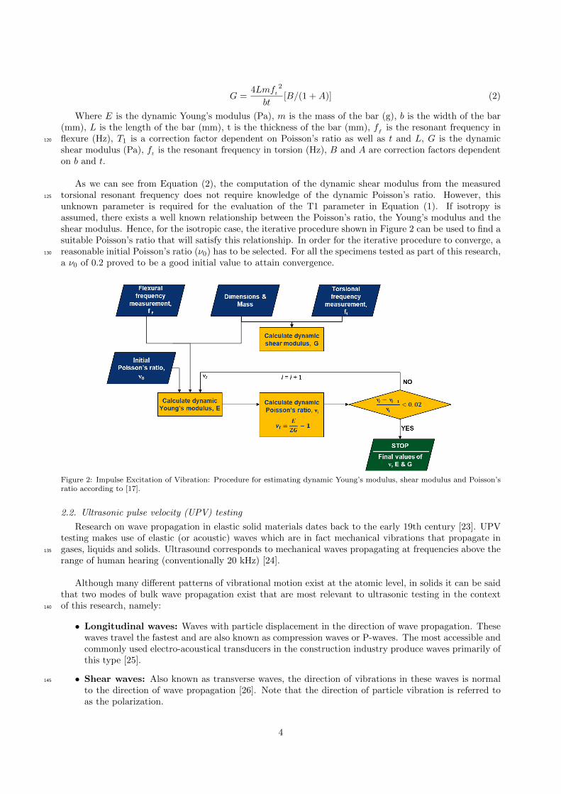
As we can see from Equation (2), the computation of the dynamic shear modulus from the measuredtorsional resonant frequency does not require knowledge of the dynamic Poisson’s ratio. However, this125

unknown parameter is required for the evaluation of the T1 parameter in Equation (1). If isotropy isassumed, there exists a well known relationship between the Poisson’s ratio, the Young’s modulus and theshear modulus. Hence, for the isotropic case, the iterative procedure shown in Figure 2 can be used to find asuitable Poisson’s ratio that will satisfy this relationship. In order for the iterative procedure to converge, areasonable initial Poisson’s ratio (ν0) has to be selected. For all the specimens tested as part of this research,130

a ν0 of 0.2 proved to be a good initial value to attain convergence.

Figure 2: Impulse Excitation of Vibration: Procedure for estimating dynamic Young’s modulus, shear modulus and Poisson’sratio according to [17].

2.2. Ultrasonic pulse velocity (UPV) testing

Research on wave propagation in elastic solid materials dates back to the early 19th century [23]. UPVtesting makes use of elastic (or acoustic) waves which are in fact mechanical vibrations that propagate ingases, liquids and solids. Ultrasound corresponds to mechanical waves propagating at frequencies above the135

range of human hearing (conventionally 20 kHz) [24].

Although many different patterns of vibrational motion exist at the atomic level, in solids it can be saidthat two modes of bulk wave propagation exist that are most relevant to ultrasonic testing in the contextof this research, namely:140

• Longitudinal waves: Waves with particle displacement in the direction of wave propagation. Thesewaves travel the fastest and are also known as compression waves or P-waves. The most accessible andcommonly used electro-acoustical transducers in the construction industry produce waves primarily ofthis type [25].

• Shear waves: Also known as transverse waves, the direction of vibrations in these waves is normal145

to the direction of wave propagation [26]. Note that the direction of particle vibration is referred toas the polarization.

4

2.2.1. Wave propagation in isotropic media

The micro-structure of many engineering materials is formed from many randomly oriented grains whichresults in the mechanical properties being independent of direction on the macroscopic scale. These materials150

are therefore isotropic. In the case of ultrasonic wave propagation, when the ultrasonic wavelength is muchgreater than the grain size, isotropic assumptions are quite valid [27]. Under these circumstances, bulk wavespropagate with equal velocity in every direction. Hence, in an infinitei isotropic material, wave energy mayonly propagate in two modes: longitudinal or shear. The equation of motion for an elastic isotropic solid canbe decomposed into the following two wave equations relating the velocity of propagation of a longitudinal155

wave (cl) and of a shear wave (cs) to the material density ρ and the two constants used in Hooke’s law foran elastic isotropic material (Young’s Modulus E and Poisson’s ratio ν) [27, 29].

cl =

(E(1 − ν)

ρ(1 + ν)(1 − 2ν)

) 12

(3)

cs =

(E

2ρ(1 + ν)

) 12

(4)

However, if a wave encounters a boundary separating two media with different properties, part of thedisturbance is reflected and part is transmitted into the second medium [23]. Similarly, if a body has a finitecross-section which is comparable to the wavelength of the disturbance, waves can bounce back and forth160

between the bounding surfaces. Such circumstances can significantly increase the complexity of analysing therecorded wave signals and relating dynamic elastic properties of the material to travel time measurements.This extra layer of complexity can be avoided by selecting the frequency of the signal generated by theultrasonic transducer, as described in detail in Section 3.3.1.

2.2.2. Standard test methods165

As previously mentioned, UPV testing in the construction industry has traditionally been limited toP-wave measurements mainly used for inspection and quality control. As such, the most relevant standardsfor the purpose of this investigation only cover determination of the propagation velocity of ultrasonic lon-gitudinal waves in hardened concrete (EN 12504-4:2004 [30] and ASTM C597 [18]). Although the ASTMstandard presents the relationship shown in Equation (3), it clearly states that the method should not be170

considered an adequate test for establishing compliance of the modulus of elasticity of field concrete withthat assumed in the design. One of the reasons for this is that the relationship described in Equation (3)requires knowledge of the dynamic Poisson’s ratio to determine the dynamic Young’s modulus from the pulsevelocity. Since the ASTM C597 standard is concerned only with determination of the velocity, it providesno indication of how to determine the Poisson’s ratio.175

The standard test method makes use of a pulse generator, a pair of electro-acoustical transducers, anamplifier, a time measuring circuit and a time display unit as shown in Figure 3.

Figure 3: Ultrasonic Pulse Velocity: Test set-up according to ASTM C597 [18]

iNote that in this context, infinite media means that boundaries have no influence on wave propagation [28].

5

It is stated that for best results, the transducers should be located directly opposite each other. Thedistance between centres of transducer faces must be measured, and the pulse velocity can then be calculated180

by dividing this distance by the pulse transit time measured using the apparatus as shown in Figure 3.

2.2.3. Wave propagation in anisotropic media

Previous research indicates that bricks formed by extrusion can exhibit a significant level of anisotropy[31]. Wave propagation in anisotropic media is substantially different from the isotropic case. The most sig-nificant difference is that elastic waves propagate with a velocity that depends on direction [27]. Moreover,185

the number of independent constants which define the elastic behaviour of the material itself will be greaterthan 2 and will depend on the symmetry class or type of anisotropy assumed. Assuming an orthotropicmaterial will result in 9 independent elastic constants while assuming transverse isotropy (material with aplane of isotropy) will result in 5. Furthermore, unlike the isotropic case, the wave modes are not necessarilypure modes as the particle vibration is neither parallel nor perpendicular to the propagation direction [27].190

In practice however, the anisotropic modes do show similarities to the isotropic modes and in these casesare referred to as quasi-longitudinal and quasi-shear. The quasi-shear modes are distinguished further bywhether they are primarily horizontally (SH-waves) or vertically (SV-waves) polarized.

Christoffel’s equations can be used to relate measured ultrasonic pulse velocities to the elastic constants.195

These expressions and related experimental procedures are not discussed here but a thorough description isgiven in [29]. However, because the propagation of a wave along a specific plane does not depend on all theelastic constants used in the material definition, the experimental procedure has to include measurementsacross different planes. Moreover, the velocities of three wave modes (P-waves, SH-waves and SV-waves)need to be measured across each of these planes in order to determine the elastic constants. Hence, the200

full elastic characterisation of an anisotropic material cannot be directly determined using P-wave velocitymeasurements alone.

3. Experimental program

The experimental campaign was carried out at the Laboratory of Technology of Structures and BuildingMaterials of the Universitat Politecnica de Catalunya (UPC-BarcelonaTech). This section presents infor-205

mation about the material components, the preparation of the specimens and the testing procedures.

3.1. Materials tested

7 different groups of solid bricks were tested in order to investigate different types of materials, both usedin existing and new constructions. 5 of these groups (I(a), I(b), III, V(a) and V(b)) consisted of handmadebricks formed by moulding. Of these, 2 groups (I(a) and I(b)) consisted of solid terracotta bricks, tested210

after production, before use in any construction project. On the other hand, group III bricks have beenextracted from an industrial complex built in the early 20th Century, part of Barcelona’s industrial heritage.Bricks from group V(a) and V(b) were extracted from a typical residential building located in Rambla deCatalunya, a street in the centre of Barcelona. It should be noted that the UPV testing procedure forspecimens from group V(b) consisted of less measurements (more detail is given in Section 3.3.3). The 2215

groups of solid bricks manufactured using a conventional extrusion process (II and IV) were both testedbefore use in any construction project. The type of bricks from group II have been used to build timbrelvaults in an ongoing construction project in Barcelona. Finally, bricks from group IV are manufacturedusing an automated process and are compliant with the EN 771-1:2011 standard [32]. A brief summary ofthe different groups tested is given in Table 1.220

6

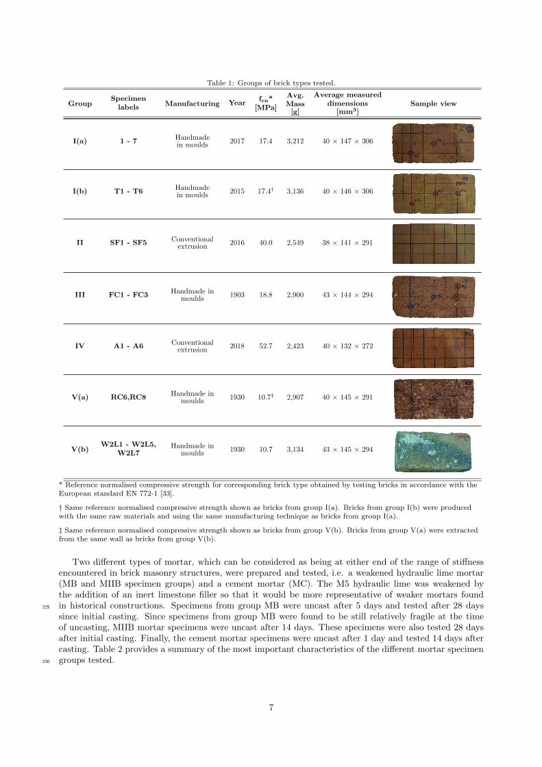
Table 1: Groups of brick types tested.

GroupSpecimen

labels Manufacturing Yearfcn*

[MPa]

Avg.Mass

[g]

Average measureddimensions

[mm3]Sample view

I(a) 1 - 7 Handmadein moulds

2017 17.4 3,212 40 × 147 × 306

I(b) T1 - T6 Handmadein moulds

2015 17.4† 3,136 40 × 146 × 306

II SF1 - SF5 Conventionalextrusion 2016 40.0 2,549 38 × 141 × 291

III FC1 - FC3 Handmade inmoulds

1903 18.8 2,900 43 × 144 × 294

IV A1 - A6 Conventionalextrusion

2018 52.7 2,423 40 × 132 × 272

V(a) RC6,RC8 Handmade inmoulds 1930 10.7‡ 2,907 40 × 145 × 291

V(b)W2L1 - W2L5,

W2L7Handmade in

moulds 1930 10.7 3,134 43 × 145 × 294

* Reference normalised compressive strength for corresponding brick type obtained by testing bricks in accordance with theEuropean standard EN 772-1 [33].

† Same reference normalised compressive strength shown as bricks from group I(a). Bricks from group I(b) were producedwith the same raw materials and using the same manufacturing technique as bricks from group I(a).

‡ Same reference normalised compressive strength shown as bricks from group V(b). Bricks from group V(a) were extractedfrom the same wall as bricks from group V(b).

Two different types of mortar, which can be considered as being at either end of the range of stiffnessencountered in brick masonry structures, were prepared and tested, i.e. a weakened hydraulic lime mortar(MB and MIIB specimen groups) and a cement mortar (MC). The M5 hydraulic lime was weakened bythe addition of an inert limestone filler so that it would be more representative of weaker mortars foundin historical constructions. Specimens from group MB were uncast after 5 days and tested after 28 days225

since initial casting. Since specimens from group MB were found to be still relatively fragile at the timeof uncasting, MIIB mortar specimens were uncast after 14 days. These specimens were also tested 28 daysafter initial casting. Finally, the cement mortar specimens were uncast after 1 day and tested 14 days aftercasting. Table 2 provides a summary of the most important characteristics of the different mortar specimengroups tested.230

7

Table 2: Groups of mortar types tested.

GroupSpecimen

labelsMix

proportions

fcn*(28 days)

[MPa]

Avg.Mass

[g]

Average measureddimensions

[mm3]Sample view

MB MB1 - MB5 Lime : filler : water1 : 0.64 : 0.37 2.3 2,930 41 × 139 × 290

MIIB MIIB1 - MIIB8 Lime : filler : water1 : 0.64 : 0.37 2.0 3,237 42 × 139 × 290

MC MC1 - MC5 Cement : sand : water1 : 3 : 0.5

49.3 3,632 41 × 139 × 291

* Reference normalised compressive strength for corresponding mortar type obtained by testing prismatic specimens inaccordance with the European standard EN 1015-11 [34].

3.2. Impulse excitation of vibration testing

3.2.1. Testing equipment

For each IEV test, a suitable data acquisition system able to record the vibrations of the specimen wasrequired so that the resonant frequency could then be extracted from the resulting acceleration-time history.The data acquisition system designed for these tests consisted of a lightweight (25 g) triaxial integrated235

circuit piezoelectric accelerometer, a signal conditioner (PCB 482A16) and an embedded real-time controller(cRIO-9064) equipped with a vibration input module (NI-9234). During testing, the real-time controllerwas connected to a laptop equipped with a program specifically created for these acquisitions using theLabVIEW 2016 programming environment from National Instruments [35].

3.2.2. Specimen preparation240

It is clear from Equation (1) that the accuracy of the estimated dynamic elastic modulus is highly de-pendent on the regularity of the specimen and the uncertainty related to its dimensions. For instance, sincethe thickness and length variables in the modulus equation have an exponent of 3, an error of 1% in thesedimensions would result in an error of 3% in the estimated modulus. Hence, in order to reduce the variationsin dimensions within each specimen, the surfaces of brick specimens were polished in order to regularise the245

faces.

It is important to note that moisture content of the specimens can have an effect on the observed resonantfrequency and hence on the estimated dynamic elastic properties. In order to control this parameter, allspecimens were dried at 120 C in a drying oven until the mass was constant as recommended in [36] before250

the execution of any tests.

Preparation of specimens also entailed marking the lines along which each specimen should be supportedduring testing to isolate the fundamental flexural and torsional modes. Finally, the impact and sensorlocations were also marked as shown in Figure 4 in order to facilitate mounting of the sensor and ensure255

consistent impulse excitations.

8

Figure 4: Markings made on every specimen prior to IEV testing.

3.2.3. Test set-up

Simple custom rigid supports were fabricated in order to isolate the flexural and torsional modes. For alltests, the supports were placed on isolation pads in order to prevent ambient vibrations from being pickedup by the accelerometer. The supports were metallic and had a sharp edge in contact with the specimen260

along the nodal lines. The supports can be seen in Figure 5 which also shows the test set-ups used forflexural (a) and torsional (b) IEV tests on whole bricks.

Figure 5: (a) Test set-up for flexural IEV test (view from top and front). (b) Test set-up for torsional IEV test (view from top,front and side).

For all tests on bricks, the accelerometer was fixed using an adhesive mounting technique via a lightweight(18 g) aluminium mounting plate fixed to the brick’s surface using a 2-component cold curing superglue.This ensured adequate vibration transmissibility while also reducing any mass loading effects (see Figure 5).265

Although this technique proved to impart very little damage on most bricks, removal of the mounting platedid cause some loss of material from the surface of many bricks. This loss of material proved to be quitesignificant in the case of the fragile MB Mortars. Since one of the secondary aims of this research campaign isto keep the specimens as intact as possible for further testing, a less intrusive mounting method was desirable,particularly for the more fragile lime mortar specimens. Hence, a different mounting technique was tested270

which involved fixing the accelerometer on the surface of the specimen using scrim-backed adhesive tapeas shown in Figure 6. Naturally, this technique further reduces any mass loading effects since the mass of

9

the adhesive tape is much lower than that of the mounting plate. However, since it is a less commonlyused mounting technique than the aforementioned one, the adequacy of its vibration transmissibility hadto be verified for the purpose of these tests. In order to achieve this, a comparative study was carried out275

between the two mounting methods on all the specimens from the MB mortar group. The observed resonantfrequency was found to differ by less than 1.2% across all the specimens. Hence, the mounting techniquewith the scrim-backed adhesive tape was used to test all mortar specimens to avoid any further damage tothe specimens.

Figure 6: Accelerometer mounting using scrim-backed adhesive tape for (a) flexural test set-up and (b) torsional test set-up ofIEV tests.

Another important consideration before testing any specimens involves selecting an appropriate sampling280

frequency to be used for all the tests. Based on the capabilities of every element of the data acquisitionsystem, a sufficiently high sampling frequency must be chosen to prevent any aliasing. This requires anestimation of the expected resonant frequencies that need to be measured. In the case of the specimenstested for this research campaign, the observed resonant frequencies varied from 586 Hz to 1794 Hz for theflexural tests and from 746 Hz to 2099 Hz for the torsional tests. A sampling frequency of 20 kHz was used285

for all the IEV tests.

3.2.4. Testing procedure

Before actually executing the vibration tests, the mass and dimensions of each specimen had to be deter-mined accurately for consequent computation of the dynamic elastic properties. The mass was determinedusing an electronic balance with a precision of 0.5 g, satisfying the 0.1% of specimen mass requirement290

stipulated in the ASTM standard [17] for all specimens tested. Each dimension was taken as the average ofmultiple readings along each of them at the locations shown in Figure 7. These measurements were takenwith a Vernier caliper with a precision of 0.02 mm. The multiple measurements were not only used tocompute the average dimensions but also to quantify the variation in dimensions of the specimens. The co-efficients of variation of all dimensions of all specimens were found to be less than 2% except for 6 specimens295

which had coefficients of variations of less than 4% for the measured thickness dimensions.

Figure 7: Locations of the 20 measurements taken with a Vernier caliper for every specimen tested under IEV. (a) 6 measure-ments of the length taken for every specimen. (b) 6 measurements of the width taken for every specimen. (c) 8 measurementsof the thickness taken for every specimen.

Once the set-ups described in the previous section have been prepared, the IEV tests simply involveapplying an impulse at the specified location using an impact tool which satisfies the requirements statedin [17]. In practice, the size and geometry of the tool depends on the size and weight of the specimen andthe force needed to produce vibration. In the case of the bricks, one of the most important considerations300

10

was to ensure that the impact was not too strong for the higher amplitudes of the recorded signals not tofall outside the measurable range of the accelerometer (±5 g).

For each IEV test, the vibration signals were recorded whilst the specimen was impacted several times(see Figure 8). An appropriate feature extraction procedure needed to be implemented in order to extract305

the resonant frequency from the acceleration-time histories. It should be noted that one of the requirementsfrom the ASTM standard [17] is to determine the resonant frequency as the average of five consecutivereadings which lie within 1% of each other. Because of this requirement, it was essential to be able toestimate the resonant frequency during testing itself. Hence, the Frequency Domain Decomposition (FDD)technique was used, because it does not only allow fast estimation of the resonant frequency but also exploits310

the data recorded from the 3 channels of the tri-axial accelerometer for improved accuracy. A custom scriptfor processing the files generated by the LabVIEW acquisition program and subsequently carrying out FDDanalysis was created in the MATLAB R© computing environment [37] by modifying the original FDD scriptby [38]. This process is summarised in Figure 8.

Figure 8: Top: Acceleration-time history for a single IEV test (with a zoom-in of a single impulse shown). Bottom: Selectionof peak during FDD process.

Once the resonant frequencies were extracted, Equations (1) and (2) could be used to estimate the315

dynamic Young’s modulus and shear modulus respectively. The iterative procedure described in Section 2.1was used to estimate the dynamic Poisson’s ratio and update the dynamic Young’s modulus accordingly.

11

3.3. Ultrasonic pulse velocity testing

3.3.1. Testing equipment

The ultrasonic pulse travel times were recorded using a PROCEQ Pundit R© PL-200 [39] commercial320

ultrasonic testing instrument. This equipment incorporates a pulse generator, receiver amplifier and timemeasuring circuit into one unit with a touch-screen display that can be used to view the waveform of recordedsignals and pulse travel time in real-time. Different transducers can be used with this instrument, each ofwhich is better suited for different applications.

325

The selection of the appropriate transducer is largely dependent on grain size and on the dimensionsof the test object. The frequency of the transducer should be chosen so that the resulting ultrasonic pulsehas a wavelength smaller than the minimum lateral dimension of the test specimen but at least twice aslarge as the grain size [39]. Since the wavelength is dependent on the velocity of propagation (wavelengthequals velocity divided by frequency), the selection of an appropriate transducer before testing the material330

is not so straightforward. It is known that the ultrasonic pulse velocity in concrete ranges from 3000 m/sto 5000 m/s [39]. Most materials tested as part of this campaign are characterised by lower velocities. Infact, the observed velocities vary from 1132 m/s (Type V(b) brick) to 4270 m/s (CM Mortar). A pairof 250 kHz transducers was used for all the UPV tests carried out as part of this research, resulting inwavelengths ranging from 5 mm to 17 mm. These wavelengths are all smaller than 38 mm, the smallest335

thickness encountered across all specimens. Although this range of wavelengths can also be considered asbeing greater than the average grain size of the materials under test, in some cases, the specimens containedsignificant heterogeneities such as voids or aggregates that are larger than the aforementioned wavelengthrange. Moreover, the specimens characterised by lower ultrasonic pulse velocities also turn out to be themost heterogeneous. This results in a greater likelihood of scattering affecting the reliability of the results340

for these specimens, since the wavelengths of the ultrasonic pulses are smaller while the effective grain sizecan be considered as being larger due to the heterogeneities. Taking multiple readings at different locationscan help to improve the reliability of results in such cases.

3.3.2. Treatment of specimens

Besides using a coupling gel between the transducers and the material during testing, the surfaces of the345

bricks were polished beforehand to ensure a smooth surface and hence prevent excessive loss of signal dueto inadequate acoustic coupling. Since all the mortar specimens were cast in specifically designed moulds,their surfaces were adequately smooth and no further polishing was carried out.

As is the case for IEV tests, moisture content of the specimens is another factor that can influence UPV350

results. Hence, to control this parameter, all measurements were made on oven-dried specimens which hadbeen allowed to stabilise to room temperature.

The final preparation step before executing the UPV tests involved marking the locations through whichthe velocity will be measured in order to be able to accurately position the transducers and measure the355

corresponding path lengths. A 4×8 grid of equal divisions on the largest faces of each specimen was usedto locate all path lengths across the length, width and thickness (see Figure 4).

3.3.3. Testing procedure

Before any UPV tests were carried out, the mass and dimensions measured for the IEV tests were usedto compute the density of the specimen which is required to evaluate the dynamic Young’s modulus using360

Equation (3).

All measurements of pulse transit times were carried out using direct transmission with the transducersarranged directly opposite each other, widely considered as the optimum configuration for accurate pulsevelocity determination. Using the UPV evaluated in this way into Equation (3) can be considered as giving365

a very localised estimate of the elastic properties since the velocity is only representative of the path alongwhich the pulse travelled. Since it is known that many types of brick masonry constituents can have asignificant level of heterogeneity, and even anisotropy in some cases, it is important to determine the pulsevelocity at multiple locations and even across different directions before utilising them to evaluate the elasticconstants describing the overall material behaviour. For the purpose of this research, three different vari-370

ables were defined to describe the elastic moduli computed from multiple pulse velocities evaluated acrossthe three different directions of each brick-sized specimen (length, width and thickness). They will hereafter

12

be referred to as EUPV,L, EUPV,W and EUPV,T .

For the UPV tests across the length and width of specimens, the reported pulse transit time at a single375

location was taken as the average of five consecutive readings with a coefficient of variation of less than 2%to reduce the effect of any measurement errors. The pulse transit time was measured at 3 locations acrossthe length as shown in Figure 9 and 3 locations across the width as shown in Figure 10. The path lengthsat these locations were measured using a Vernier caliper and the pulse velocity was computed by dividingthe path length by the transit time. EUPV,L was then computed from Equation (3) using the average of the380

computed velocities from the 3 length locations specified and the Poisson’s ratio estimated from the IEVtests. EUPV,W was computed using exactly the same procedure but using the velocities computed from thetransit times and path lengths measured across the width.

Figure 9: Locations of ultrasonic pulse travel time measurements across length: (a) Top quarter, (b) Middle, (c) Bottomquarter.

Figure 10: Locations of ultrasonic pulse travel time measurements across width: (a) Top quarter, (b) Middle, (c) Bottomquarter

Specimens from group V(b) were tested before the methodology described herein had been developed.As such, for specimens from group V(b), the transit time was only measured at the middle location across385

the length and the width. Moreover, no measurements of pulse transit times were taken across the thicknessof specimens from this group.

For all other specimens, the procedure used for computing EUPV,T differed from that used for EUPV,L

and EUPV,W . Due to the shorter distance of the path length, it was expected that the effect of heterogeneities390

and scattering would be more significant. As such, the pulse transit time across the thickness was measuredat 32 different locations on the face of each specimen as shown in Figure 11. The 32 measurements were usedto generate travel time contour maps which could also be used to assess the heterogeneity of each specimen.In order to minimise the effect of any measurement errors, two consecutive sets of 32 readings were taken foreach specimen and corresponding readings that differed by more than 2% were eliminated from any further395

computation. Since taking 32 measurements of path length was both time-consuming and impractical (partsat the centre of specimens were difficult to access to measure accurately), the pulse velocity was computedby dividing the average of the 8 thickness measurements taken as part of the IEV procedure by the averageof the 32 measurements of pulse transit times. EUPV,T was then computed for each specimen from thiscomputed velocity and using the Poisson’s ratio estimated from IEV testing.400

13

Figure 11: (a) Measurement of ultrasonic pulse transit time across thickness. (b) Example of an ultrasonic travel time colourmap generated from 32 measurements over the face of each specimen.

4. Results and discussion

As described in Section 2.1, the dynamic Young’s modulus (EIEV ), shear modulus (GIEV ) and Pois-son’s ratio (νIEV ) for each specimen were computed from the measured mass, dimensions and fundamentalfrequencies by direct application of Equations (1) and (2) through the procedure described in Figure 2. Theaverage of these results for each specimen group are presented in Table 3.405

Table 3: Final estimated dynamic elastic properties from IEV testing.

SpecimenGroup

No. ofspecimens

tested

Average values

EIEV

[MPa]coeff. ofvariation

GIEV

[MPa]coeff. ofvariation

νIEV

[MPa]coeff. ofvariation

35 UnitsI(a) 7 7,882 15% 3,530 15% 0.12 14%I(b) 6 7,931 17% 3,628 17% 0.09 41%II 5 18,313 1% 7,240 1% 0.26 7%III 3 7,107 13% 3,309 10% 0.07 31%IV 6 15,505 1% 5,733 1% 0.35 5%

V(a) 2 5,475 8% 2,525 5% 0.08 31%V(b) 6 4,068 30% 1,965 29% 0.03 70%

21 MortarMB 5 3,987 10% 1,811 9% 0.10 16%

MIIB 8 4,269 6% 1,886 6% 0.12 24%MC 8 28,954 5% 11,417 3% 0.27 8%

As can be expected, in the case of bricks, the specimens produced by extrusion (groups II and IV) havehigher values of dynamic Young’s and shear moduli. This is because they are generally of higher quality andless porous than the bricks handmade in moulds and therefore exhibit a more stiff elastic behaviour. Simi-larly, the more modern cement mortar specimens appear to be much more stiff than the weaker lime mortars.

410

In addition to the estimates of the dynamic properties from IEV tests, dynamic Young’s moduli for everyspecimen were also computed using Equation (3) from the average ultrasonic pulse velocity across differentdirections, derived as described in Section 3.3. This results in three estimates of the dynamic Young’smodulus from UPV tests for every specimen, corresponding to its three main dimensions (EUPV,L, EUPV,W

and EUPV,T ). The average of these results for each specimen group are presented in Table 4.415

14

Table 4: Estimated dynamic Young’s modulus from UPV measurements across different directions.

SpecimenGroup

No. ofspecimens

tested

Average values

EUPV,L

[MPa]coeff. ofvariation

EUPV,W

[MPa]coeff. ofvariation

EUPV,T

[MPa]coeff. ofvariation

35 UnitsI(a) 7 7,837 18% 8,241 19% 5,764 20%I(b) 6 7,938 13% 8,189 15% 5,979 17%II 5 13,756 4% 15,199 4% 8,924 5%III 3 7,305 2% 8,717 7% 8,016 15%IV 6 9,157 8% 7,109 8% 12,035 8%

V(a) 2 5,498 4% 6,336 7% 5,754 14%V(b) 6 4,604 35% 5,538 22% - -

21 MortarMB 5 4,527 6% 5,686 7% 6,230 7%

MIIB 8 4,887 16% 6,486 4% 6,123 2%MC 8 28,601 4% 30,125 6% 29,236 4%

One of the most useful applications of the estimated dynamic Young’s moduli across different directionsis to evaluate if the specimens are actually isotropic. As such, a comparison of the relative scatters betweenthese estimated properties for every specimen group is summarised in Table 5. The scatters are normalisedto EUPV,L which can be considered the most reliable estimate from UPV tests carried out as part of thisresearch. This is due to the fact that it is computed from the pulse velocity determined across the largest420

dimension of the specimens, hence minimising the effects of localised heterogeneities as well as those ofmeasurement errors.

As described in Section 3.3.3, the 32 measurements of pulse transit time across the thickness cover almostthe whole area over the two largest opposing faces of each specimen. Hence, for each set of readings, the425

maximum variation of the pulse transit times measured across the thickness (∆tT = tT,max − tT,min) canprovide an indication of the level of heterogeneity for each specimen. As mentioned in Section 3.3.3, twoconsecutive sets of readings were taken for each specimen. Therefore the representative maximum variationof each specimen (∆tT,spec) was taken as the average of ∆tT,1 and ∆tT,2. Similarly, the representativeaverage measured pulse transit time of each specimen (tT,spec) was taken as the average of tT,1 and tT,2. In430

order to allow adequate comparisons between specimens, a unitless heterogeneity measure for each specimen(HMspec) was computed as follows:

HMspec =∆tT,spec

tT,spec(5)

Subsequently, the heterogeneity measure for a specimen group (HMGroup) was computed as the averageof the HMspec values of all specimens belonging to that group. These values are presented in the last columnof Table 5.435

Table 5: Comparison of dynamic Young’s modulus from UPV measurements across different directions and heterogeneitymeasure for each specimen group.

SpecimenGroup

No. ofspecimens

tested

Average valuesHMGroup

EUPV,L−EUPV,W

EUPV,L

EUPV,L−EUPV,T

EUPV,L

EUPV,W −EUPV,T

EUPV,L

35 UnitsI(a) 7 -5% 26% 32% 24%I(b) 6 -3% 25% 28% 22%II 5 -10% 35% 46% 10%III 3 -19% -10% 10% 26%IV 6 22% -31% -54% 8%

V(a) 2 -15% -5% 11% 26%V(b) 6 -20% - - -

21 MortarMB 5 -26% -38% -12% 16%

MIIB 8 -33% -25% 7% 11%MC 8 -5% -2% 3% 9%

15

The comparisons in Table 5 reveal that the bricks produced by extrusion (groups II and IV) display ahigher level of anisotropy since the relative scatters between estimated dynamic Young’s moduli for differ-ent directions were consistently greater for specimens from these two groups. It should be noted that theaverage values of the relative scatters between the estimated dynamic Young’s moduli for specific directionsalso appear to be significant for some of the other specimen groups tested (I(a), I(b), MB, MIIB). However,440

there are much greater variations in these relative scatters among individual specimens from these groupswhen compared to the variations among the specimens from groups II and IV. This can be expected dueto the greater homogeneity of the bricks manufactured by extrusion, confirmed by the significantly lowergroup heterogeneity measures (see Table 5). It is clear to see that although the comparison of estimateddynamic Young’s moduli from ultrasonic P-wave velocities in different directions can provide some infor-445

mation on the inherent anisotropy of the material, it can be misleading and hence requires very carefulinterpretation. Moreover, as described in Section 2.2.3, the wave modes are not necessarily pure modes inanisotropic media. Therefore, the ratios of the estimated dynamic moduli from P-wave velocities betweendifferent directions do not necessarily reflect the actual ratios between elastic constants of the material. Infact, for the anisotropic case, estimating the dynamic elastic modulus from traditional ultrasonic P-wave450

testing alone can be considered unreliable.

Comparing the dynamic Young’s modulus evaluated from IEV testing with that evaluated from UPVtesting with P-waves across the length of the specimens can be considered a more robust way of evaluatingthe reliability of the results from UPV testing. In theory, the stresses developed during testing with these455

two methods should be resisted across the same material direction as illustrated in Figure 12.

Figure 12: Schematic representation of (a) stresses in material during flexural IEV test, (b) stresses in material during UPVtesting across length.

Table 6 presents the relative scatter between EIEV and EUPV,L for each specimen group.

Table 6: Comparison of dynamic Young’s modulus from IEV and UPV measured across length.

SpecimenGroup

No. ofspecimens

tested

Average values

EIEV

[MPa]coeff. ofvariation

EUPV,L

[MPa]coeff. ofvariation

EIEV −EUPV,L

EIEV

35 UnitsI(a) 7 7,882 15% 7,837 18% 1%I(b) 6 7,931 17% 7,938 13% -0.1%II 5 18,313 1% 13,756 4% 25%III 3 7,107 13% 7,305 2% -3%IV 6 15,505 1% 9,157 8% 41%

V(a) 2 5,475 8% 5,498 4% -0.4%V(b) 6 4,068 30% 4,604 35% -13%

21 MortarMB 5 3,987 10% 4,527 6% -14%

MIIB 8 4,269 6% 4,887 16% -14%MC 8 28,954 5% 28,601 4% 1%

From Table 6, it is clear that the differences between EIEV and EUPV,L are significantly greater forspecimens from group II and IV when compared to the differences for specimens from any other group ofconstituent materials tested. This suggests that values of dynamic Young’s modulus evaluated from UPV460

testing only with P-waves is unreliable for bricks produced by extrusion due to their apparent anisotropy.Hence, the comparison of EIEV and EUPV,L has brought us to the same conclusion as the comparison ofthe dynamic Young’s moduli estimated from ultrasonic compression wave velocities across different direc-tions. However, in this case, the disagreement between EIEV and EUPV,L is much more apparent and the

16

comparison does not lend itself to misinterpretation.465

From a more general perspective, it is clear that the bricks manufactured through an extrusion process(groups II and IV) show the smallest coefficients of variation. As previously discussed, one of the mainreasons for this is that they are characterised by greater homogeneity.

470

For results from IEV testing, the estimates of dynamic Poisson’s ratio generally have greater coefficientsof variation, indicating that the evaluation of this parameter is more sensitive to heterogeneities and tochanges in testing conditions (see Table 3). Nevertheless, for specimens characterised by a more markedisotropic behaviour, it can be said that IEV testing can provide reliable estimates of the dynamic Poisson’sratio. In fact, most specimen groups have a coefficient of variation of 31% or less for this parameter with475

the exception of groups I(b) and V(b). Even so, it should be noted that the average estimated value ofthe dynamic Poisson’s ratio was quite low for both these groups of specimens. Hence, the 41% and 70%coefficients of variation among specimens from group I(b)and V(b) respectively, relate to variations of only0.04 and 0.02 respectively in the estimated Poisson’s ratio. The value of the dynamic Poisson’s ratio deter-mined for the cement mortar is significantly higher than that of the lime mortar and of the brick specimens480

handmade in moulds.

One of the main advantages of being able to determine the dynamic Poisson’s ratio reliably using IEVtesting, is that it can provide a value for a previously unknown parameter in Equation (3), used to computethe dynamic Young’s modulus from the experimentally evaluated ultrasonic compression wave velocity. In485

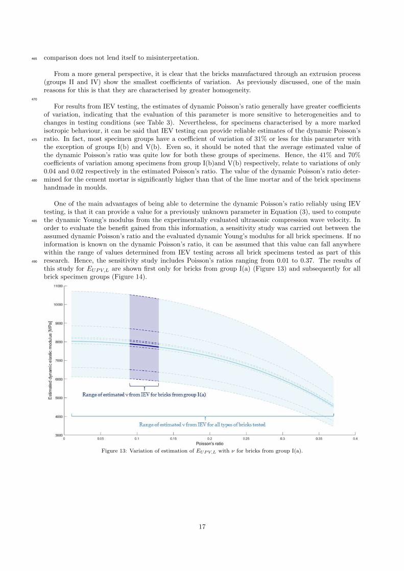
order to evaluate the benefit gained from this information, a sensitivity study was carried out between theassumed dynamic Poisson’s ratio and the evaluated dynamic Young’s modulus for all brick specimens. If noinformation is known on the dynamic Poisson’s ratio, it can be assumed that this value can fall anywherewithin the range of values determined from IEV testing across all brick specimens tested as part of thisresearch. Hence, the sensitivity study includes Poisson’s ratios ranging from 0.01 to 0.37. The results of490

this study for EUPV,L are shown first only for bricks from group I(a) (Figure 13) and subsequently for allbrick specimen groups (Figure 14).

Figure 13: Variation of estimation of EUPV,L with ν for bricks from group I(a).

17

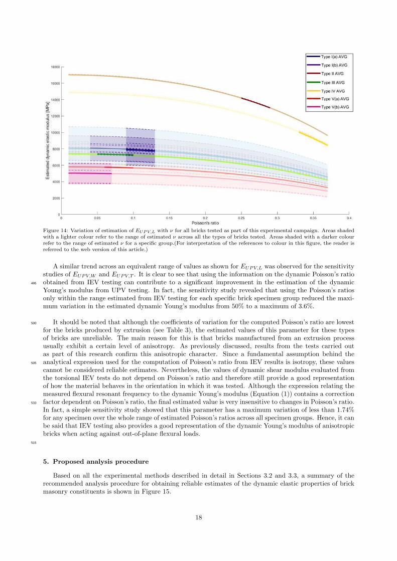
Figure 14: Variation of estimation of EUPV,L with ν for all bricks tested as part of this experimental campaign. Areas shadedwith a lighter colour refer to the range of estimated ν across all the types of bricks tested. Areas shaded with a darker colourrefer to the range of estimated ν for a specific group.(For interpretation of the references to colour in this figure, the reader isreferred to the web version of this article.)

A similar trend across an equivalent range of values as shown for EUPV,L was observed for the sensitivitystudies of EUPV,W and EUPV,T . It is clear to see that using the information on the dynamic Poisson’s ratioobtained from IEV testing can contribute to a significant improvement in the estimation of the dynamic495

Young’s modulus from UPV testing. In fact, the sensitivity study revealed that using the Poisson’s ratiosonly within the range estimated from IEV testing for each specific brick specimen group reduced the maxi-mum variation in the estimated dynamic Young’s modulus from 50% to a maximum of 3.6%.

It should be noted that although the coefficients of variation for the computed Poisson’s ratio are lowest500

for the bricks produced by extrusion (see Table 3), the estimated values of this parameter for these typesof bricks are unreliable. The main reason for this is that bricks manufactured from an extrusion processusually exhibit a certain level of anisotropy. As previously discussed, results from the tests carried outas part of this research confirm this anisotropic character. Since a fundamental assumption behind theanalytical expression used for the computation of Poisson’s ratio from IEV results is isotropy, these values505

cannot be considered reliable estimates. Nevertheless, the values of dynamic shear modulus evaluated fromthe torsional IEV tests do not depend on Poisson’s ratio and therefore still provide a good representationof how the material behaves in the orientation in which it was tested. Although the expression relating themeasured flexural resonant frequency to the dynamic Young’s modulus (Equation (1)) contains a correctionfactor dependent on Poisson’s ratio, the final estimated value is very insensitive to changes in Poisson’s ratio.510

In fact, a simple sensitivity study showed that this parameter has a maximum variation of less than 1.74%for any specimen over the whole range of estimated Poisson’s ratios across all specimen groups. Hence, it canbe said that IEV testing also provides a good representation of the dynamic Young’s modulus of anisotropicbricks when acting against out-of-plane flexural loads.

515

5. Proposed analysis procedure

Based on all the experimental methods described in detail in Sections 3.2 and 3.3, a summary of therecommended analysis procedure for obtaining reliable estimates of the dynamic elastic properties of brickmasonry constituents is shown in Figure 15.

18

Figure 15: Summary of the proposed procedure for determining dynamic elastic properties of brick masonry constituents.

As can be seen from Figure 15, the first step of the analysis process involves computing EIEV , GIEV520

and νIEV from the results of IEV tests conducted as described in Section 3.2. Following this, the resultingνIEV is used in the computation of EUPV,L, EUPV,W and EUPV,T from ultrasonic pulse velocities measuredacross different dimensions of each specimen as described in Section 3.3. The average values for each groupof specimens representing a particular type of brick or mortar can then be obtained. All subsequent analysiscan be carried out with these representative average values. Once these values have been obtained, it is525

important to assess if any of the brick or mortar types being tested exhibit a significant level of anisotropyin order to evaluate the reliability of the obtained results. If there are significant relative scatters (>30%)between EUPV,L, EUPV,W and EUPV,T as well as a significant relative scatter (>20%) between EIEV andEUPV,L then the type of brick or mortar under test can be said to be anisotropic. If this is the case, only thedynamic Young’s modulus (EIEV ) and the dynamic shear modulus (GIEV ) computed from results of IEV530

testing provide a good representation of the behaviour of the material in the respective testing orientations.On the other hand, if the material exhibits a predominantly isotropic behaviour, in theory, all the dynamicelastic material properties evaluated from IEV and UPV testing can be considered reliable. However, sincethe reliability of UPV estimates depend strongly on heterogeneity and surface roughness, if EUPV,W and/orEUPV,T differ from EUPV,L, the latter parameter can be considered as being more reliable in most cases.535

The application of this analysis process can be illustrated with two simple examples. Taking the caseof the cement mortar tested as part of this research (group MC), the relative scatters between EUPV,L,EUPV,W and EUPV,T are all of 5% or less and the relative scatter between EIEV and EUPV,L is of only 1%.In this case, it is clear that the material is isotropic and all the estimated dynamic elastic properties can540

be considered reliable. On the contrary, for the type of bricks belonging to group II, the relative scatterbetween EUPV,L and EUPV,T is 35% while that between EUPV,W and EUPV,T is 46%. Furthermore, therelative scatter between EIEV and EUPV,L turned out to be 25%. For these bricks, all properties estimatedfrom UPV tests as well as the value of νIEV cannot be considered reliable. Nevertheless, EIEV is stillrepresentative of the dynamic Young’s modulus when out-of-plane flexural loads are acting on this type of545

brick while GIEV still provides a good representation of the response of bricks of this type to torsional loads(in the same orientation as the bricks were tested).

19

6. Conclusions and future work

The research has proposed a robust procedure based on the synergy of two approaches, namely ImpulseExcitation of Vibration (IEV) and Ultrasonic Pulse Velocity (UPV) testing for the determination of the dy-550

namic elastic properties of brick masonry constituents. The influence of testing conditions and other factorsspecific to brick masonry constituents have been evaluated to assess the applicability of these techniques.At the same time, methods to mitigate possible sources of error have been explored and as a result, clearpractical provisions have been given concerning every step of the procedure from testing protocols to theinterpretation of results. Moreover, in order to derive meaningful ranges of results for different masonry555

typologies, the experimental program has explored different types of bricks and mortars. The tests haveconsidered hydraulic lime mortar, cement mortar, new bricks manufactured using either hand-made mould-ing or extrusion, and existing bricks extracted from heritage buildings in Barcelona, Spain.

The proposed methodology can be applied to whole brick specimens as well as to specifically-cast mortar560

specimens. In the case of whole brick specimens, these can be recently manufactured or extracted fromexisting constructions. In the latter scenario, the methods described in this paper cannot be considered asbeing fully non-destructive since they implicitly require the extraction of bricks from the structure. Never-theless, both methods can be used to test extracted bricks without causing any further significant damageto the material, allowing the same bricks to be re-used or to undergo further testing. In the case of mor-565

tar specimens, since they have to be cast to specific dimensions, the proposed testing procedures are notsuitable for testing mortar already present in existing masonry structures. Nevertheless, the procedures canbe applied to test freshly-cast mortar either for use in new constructions or intended for repair works. Theresults obtained from the present investigation show that the two methods (IEV and UPV) can providereliable estimates of the actual dynamic elastic properties of typical brick masonry constituents.570

For isotropic constituent materials, one of the main advantages of the proposed procedure lies in usingthe dynamic Poisson’s ratio derived from IEV tests to improve the accuracy of the dynamic Young’s modulusevaluated from conventional UPV tests based on the transmission of P-waves. Since UPV tests are simplerand faster to execute when compared to IEV tests, a possible application of this procedure could involve575

determination of the dynamic Poisson’s ratio using IEV testing on a selected number of specimens togetherwith characterisation of the dynamic Young’s modulus using UPV testing on a larger sample size. In thecase of existing single-leaf walls, this procedure may even be extended to in situ UPV tests on bricks.

The results reveal that bricks produced by a conventional extrusion procedure exhibit a significant level580

of anisotropy. In this case, the estimation of the dynamic Young’s modulus from traditional UPV tests isnot reliable since the propagation of ultrasonic waves is not governed by the same simplified rules as inisotropic media. The procedure involving the combined information from flexural and torsional IEV teststo evaluate the dynamic Poisson’s ratio is also not applicable to such bricks since it relies on the fundamen-tal assumption of isotropy. Nevertheless, IEV tests can still provide estimates of effective dynamic elastic585

moduli which define the behaviour of brick specimens when subjected to flexural or torsional loading.

An extension of the research presented herein may explore testing procedures involving ultrasonic shearwave transducers to better characterise the dynamic elastic behaviour of anisotropic bricks. Theoretically,such transducers could also be used to directly evaluate the dynamic Poisson’s ratio of isotropic constituents.590

However, it should be noted that accurately determining the arrival time of the shear wave can prove tobe especially difficult, particularly when testing brick-sized specimens of materials with significant hetero-geneities and rough surfaces.

One of the most important implications of this work is that it provides a means of better understanding595

the relationship between static and dynamic elastic properties for brick masonry constituents. This relation-ship is as of yet not well understood. Additional laboratory investigations are currently being carried out atthe Universitat Politecnica de Catalunya to correlate the static and dynamic elastic properties in differentmasonry components..

Conflicts of interest

The authors confirm that there are no known conflicts of interest associated with this publication.

20

Acknowledgements

This research has received the financial support from the MINECO (Ministerio de Economia y Com-petividad of the Spanish Government) and the ERDF (European Regional Development Fund) through theMULTIMAS project (Multiscale techniques for the experimental and numerical analysis of the reliabilityof masonry structures, ref. num. BIA2015-63882-P). Support from the AGAUR agency of the Generalitatde Catalunya, in the form of a predoctoral grant awarded to the corresponding author is also gratefullyacknowledged.

References

[1] European Committee for Standardization (CEN), EN 14580:2005. Natural stone test methods - Determination of staticelastic modulus (2005).

[2] L. Binda, C. Tiraboschi, G. Mirabella Roberti, G. Baronio, G. Cardani, Measuring masonry material properties: detailedresults from an extensive experimental research Part I: Tests on masonry components. (Report 5.1 Politecnico di Milano).,Tech. rep., Politecnico di Milano (1996).

[3] L. Binda, C. Tiraboschi, S. Abbaneo, Experimental Research to Characterise Masonry Materials, Masonry International.URL https://www.masonry.org.uk/downloads/experimental-research-to-characterise-masonry-materials/

[4] L. Binda, C. Tedeschi, P. Condoleo, Characterisation of Materials Sampled From Some My S’on Temples, in: 7th Inter-national Congress on Civil Engineering, 2006.

[5] G. Baronio, L. Binda, C. Tedeschi, C. Tiraboschi, Characterisation of the materials used in the construction of the NotoCathedral, Construction and Building Materials 17 (8) (2003) 557–571. doi:10.1016/j.conbuildmat.2003.08.007.

[6] D. V. Oliveira, Mechanical Characterization of Stone and Brick Masonry (Report 00-DEC/E-4), Tech. rep., University ofMinho (2000).

[7] D. V. Oliveira, P. B. Lourenco, P. Roca, Experimental Characterization of the Behaviour of Brick Masonry Subjected toCyclic Loading, in: 12th international Brick/Block Masonry Conference, no. May 2014, 2000, pp. 1–8.

[8] D. V. Oliveira, P. B. Lourenco, P. Roca, Cyclic behaviour of stone and brick masonry under uniaxial compressive loading,Materials and Structures/Materiaux et Constructions 39 (286) (2006) 247–257. doi:10.1617/s11527-005-9050-3.

[9] L. Pela, E. Canella, A. Aprile, P. Roca, Compression test of masonry core samples extracted from existing brickwork,Construction and Building Materials 119 (2016) 230–240. doi:10.1016/j.conbuildmat.2016.05.057.

[10] E. I. Mashinsky, Differences between static and dynamic elastic moduli of rocks: Physical causes, Russian Geology andGeophysics 44 (9) (2003) 953–959.

[11] M. Ciccotti, F. Mulargia, Differences between static and dynamic elastic moduli of a typical seismogenic rock, GeophysicalJournal International 157 (1) (2004) 474 – 477.

[12] J. Martınez-Martınez, D. Benavente, M. A. Garcıa-del Cura, Comparison of the static and dynamic elastic modu-lus in carbonate rocks, Bulletin of Engineering Geology and the Environment 71 (2) (2012) 263–268. doi:10.1007/

s10064-011-0399-y.

[13] A. R. Najibi, M. Ghafoori, G. R. Lashkaripour, M. R. Asef, Empirical relations between strength and static and dynamicelastic properties of Asmari and Sarvak limestones, two main oil reservoirs in Iran, Journal of Petroleum Science andEngineering 126 (2015) 78–82. doi:10.1016/j.petrol.2014.12.010.URL http://dx.doi.org/10.1016/j.petrol.2014.12.010

[14] W. Fei, B. Huiyuan, Y. Jun, Z. Yonghao, Correlation of Dynamic and Static Elastic Parameters of Rock, ElectronicJournal of Geotechnical Engineering 21 (04) (2016) 1551–1560.

[15] Y. Z. Totoev, J. M. Nichols, A Comparative Experimental Study of the Modulus of Elasticity of Bricks and Masonry, in:11th International Brick/Block Masonry Conference, no. October, 1997.

[16] J. M. Nichols, Y. Z. Totoev, Experimental determination of the dynamic Modulus of Elasticity of masonry units, in: 15thAustralian Conference on the Mechanics of Structures and Materials (ACMSM), 1997.

[17] ASTM, E 1876 - Standard Test Method for Dynamic Young’s Modulus, Shear Modulus, and Poisson’s Ratio by ImpulseExcitation of Vibration (2002). doi:10.1520/E1876-09.responsibility.

21

[18] ASTM, C597 - Standard Test Method for Pulse Velocity Through Concrete (2010). doi:10.1520/C0597-09.

[19] V. Brotons, R. Tomas, S. Ivorra, A. Grediaga, Relationship between static and dynamic elastic modulus of calcareniteheated at different temperatures: The San Julian’s stone, Bulletin of Engineering Geology and the Environment 73 (3)(2014) 791–799. doi:10.1007/s10064-014-0583-y.

[20] S. Dimter, T. Rukavina, K. Minazek, Estimation of elastic properties of fly ash-stabilized mixes using nondestructiveevaluation methods, Construction and Building Materials 102 (2016) 505–514. doi:10.1016/j.conbuildmat.2015.10.175.

[21] M. Asmani, C. Kermel, A. Leriche, M. Ourak, Influence of porosity on Youngs modulus and poisson’s ratio in aluminaceramics, Journal of the European Ceramic Society 21 (8) (2001) 1081–1086. doi:10.1016/S0955-2219(00)00314-9.

[22] L. E. Garcıa, Estudio experimental del comportamiento a compresion de elementos petreos confinados con materialescompuestos, Doctoral thesis, Universitat d’Alacant (2018).

[23] J. D. Achenbach, Wave propagation in elastic solids, Vol. 16, 1973. arXiv:arXiv:1011.1669v3, doi:10.1002/zamm.

19920720607.

[24] P. Laugier, G. Haıat, Chapter 2: Introduction to the Physics of Ultrasound, in: Bone Quantitative Ultrasound, 2011, pp.29–45. arXiv:arXiv:1011.1669v3, doi:10.1007/978-94-007-0017-8.

[25] J. H. Bungey, S. G. Millard, M. G. Grantham, Testing of Concrete in Structures, 1996.

[26] Z. Nazarchuk, V. Skalskyi, O. Serhiyenko, Chapter 2: Propagation of Elastic Waves in Solids, in: Acoustic Emission,Vol. i, Springer International Publishing, 2017, pp. 29–73. doi:10.1007/978-3-319-49350-3.URL http://link.springer.com/10.1007/978-3-319-49350-3

[27] C. Lane, Wave Propagation in Anisotropic Media, in: The Development of a 2D Ultrasonic Array Inspection for SingleCrystal Turbine Blades, 2014, pp. 13–39. doi:10.1007/978-3-319-02517-9_2.URL http://link.springer.com/10.1007/978-3-319-02517-9_2

[28] J. L. Rose, Ultrasonic Guided Waves in Solid Media, Cambridge University Press, New York, 2014. doi:10.1017/

CBO9781107273610.URL http://ebooks.cambridge.org/ref/id/CBO9781107273610

[29] J. L. Rose, Ultrasonic Waves in Solid Media, Cambridge University Press, 1999.

[30] European Committee for Standardization (CEN), EN 12504-4:2004. Testing concrete Part 4: Determination of ultrasonicpulse velocity (2004). doi:ConstructionStandard,CS1:2010.

[31] A. Fodi, Effects influencing the compressive strength of a solid, fired clay brick, Periodica Polytechnica Civil Engineering55 (2) (2011) 117–128. doi:10.3311/pp.ci.2011-2.04.

[32] European Committee for Standardization (CEN), EN 771-1:2011+A1:2015. Specification for masonry units Part 1: Claymasonry units (2015).

[33] European Committee for Standardization (CEN), EN 772-1. Methods of test for masonry units. Part 1: Determination ofcompressive strength (2010).

[34] European Committee for Standardization (CEN), EN 1015-11. Methods of test for mortar for masonry - Part 11: Deter-mination of flexural and compressive strength of hardened mortar (2007).

[35] National Instruments, LabVIEW 2016 Help (2016).

[36] ASTM, C 1259 - Standard Test Method for Dynamic Young ’s Modulus , Shear Modulus , and Poisson’s Ratio for AdvancedCeramics by Impulse Excitation of Vibration (2001). doi:10.1520/E1875-08.2.

[37] MathWorks, MATLAB R2017b Documentation.URL https://es.mathworks.com/help/releases/R2017b/index.html

[38] M. Farshchin, Frequency Domain Decomposition (FDD) (2015).

[39] PROCEQ, PUNDIT PL-200 Operating Instructions (2014).

22