ingreso nacional y sistema de cuentas nacionalesciep.itam.mx/~msegui/cap4b.pdf · 23 mishelle...
TRANSCRIPT

1
Mishelle Seguí ITAM, 2007 Economía II
Ingreso Nacional y Sistema de Cuentas Nacionales
n Los sistemas de CN describen la actividad económica que genera el ingreso del país y su relación con la producción y el gasto. De esta manera, mediante el SCN se expresan las características generales, las relaciones entre las variables de estructura y la magnitud de las transacciones globales de la economía nacional
2
Mishelle Seguí ITAM, 2007 Economía II
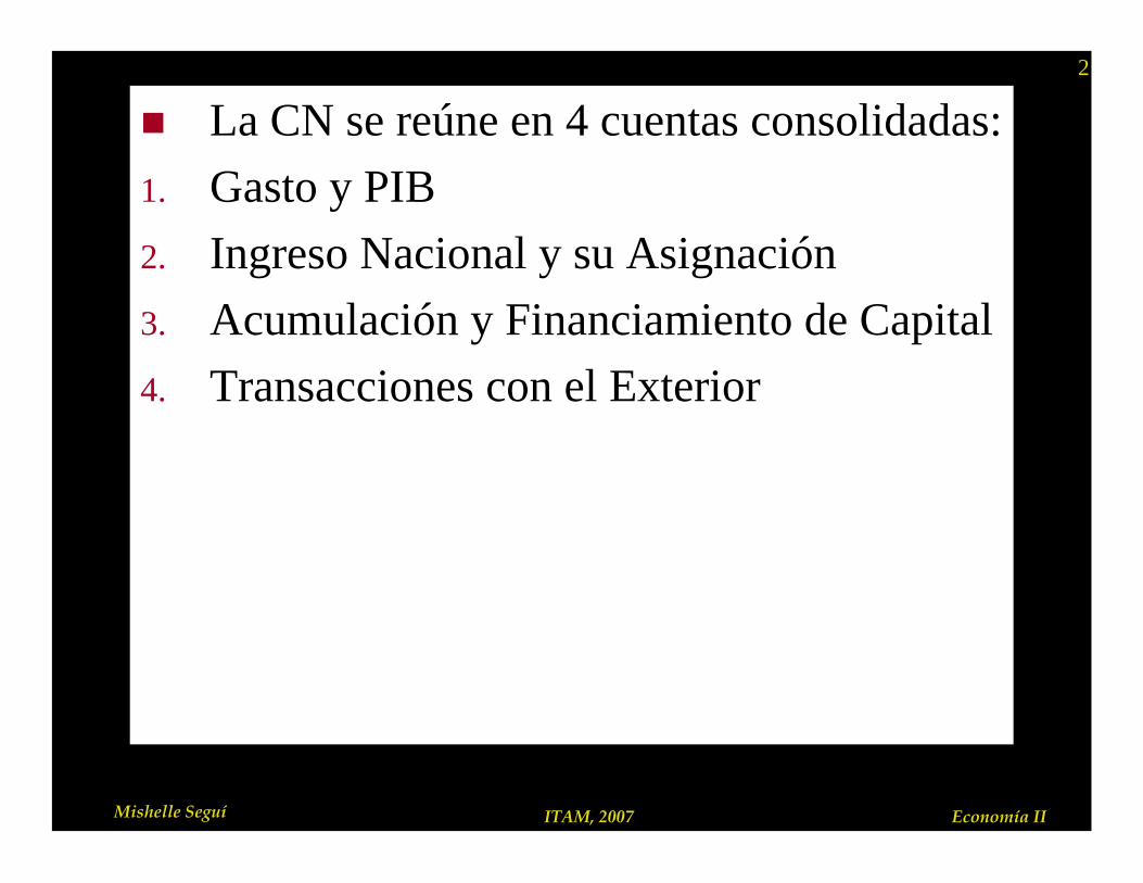
n La CN se reúne en 4 cuentas consolidadas:
1. Gasto y PIB
2. Ingreso Nacional y su Asignación
3. Acumulación y Financiamiento de Capital
4. Transacciones con el Exterior
3
Mishelle Seguí ITAM, 2007 Economía II
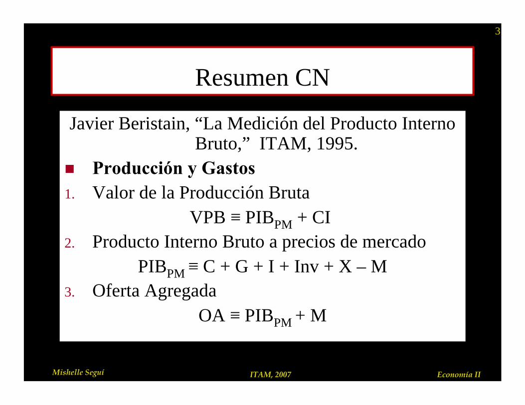
Resumen CN
Javier Beristain, “La Medición del Producto Interno Bruto,” ITAM, 1995.
n Producción y Gastos1. Valor de la Producción Bruta
VPB ≡ PIBPM + CI2. Producto Interno Bruto a precios de mercado
PIBPM ≡ C + G + I + Inv + X – M3. Oferta Agregada
OA ≡ PIBPM + M
4
Mishelle Seguí ITAM, 2007 Economía II
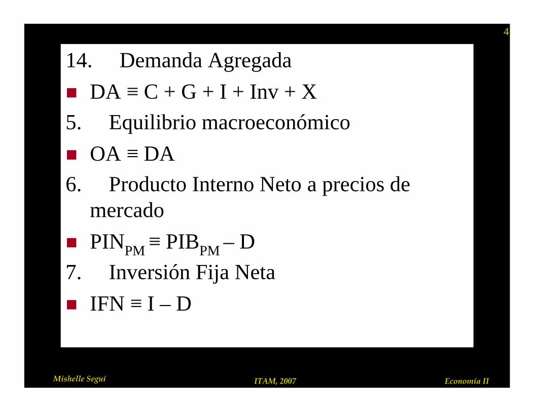
14. Demanda Agregada
n DA ≡ C + G + I + Inv + X5. Equilibrio macroeconómico
n OA ≡ DA6. Producto Interno Neto a precios de
mercado
n PINPM ≡ PIBPM – D7. Inversión Fija Neta
n IFN ≡ I – D
5
Mishelle Seguí ITAM, 2007 Economía II
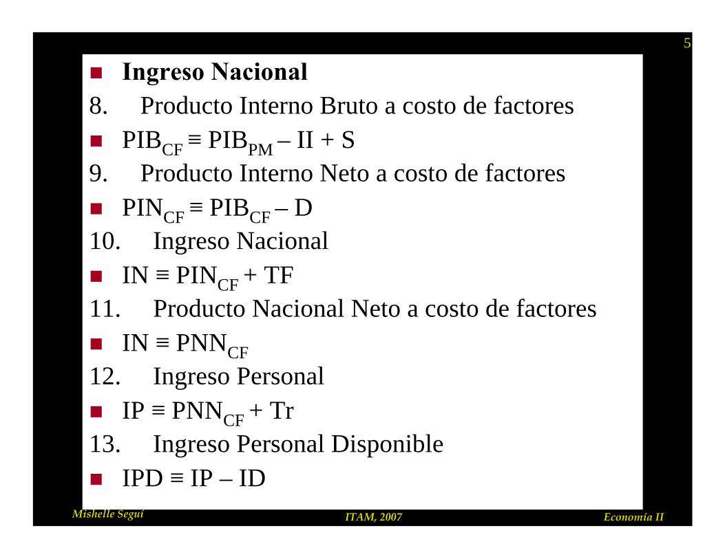
n Ingreso Nacional8. Producto Interno Bruto a costo de factoresn PIBCF ≡ PIBPM – II + S9. Producto Interno Neto a costo de factoresn PINCF ≡ PIBCF – D10. Ingreso Nacionaln IN ≡ PINCF + TF11. Producto Nacional Neto a costo de factoresn IN ≡ PNNCF
12. Ingreso Personaln IP ≡ PNNCF + Tr13. Ingreso Personal Disponiblen IPD ≡ IP – ID
6
Mishelle Seguí ITAM, 2007 Economía II
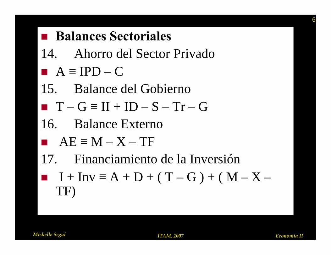
n Balances Sectoriales14. Ahorro del Sector Privadon A ≡ IPD – C15. Balance del Gobiernon T – G ≡ II + ID – S – Tr – G16. Balance Externon AE ≡ M – X – TF17. Financiamiento de la Inversiónn I + Inv ≡ A + D + ( T – G ) + ( M – X –
TF)
7
Mishelle Seguí ITAM, 2007 Economía II
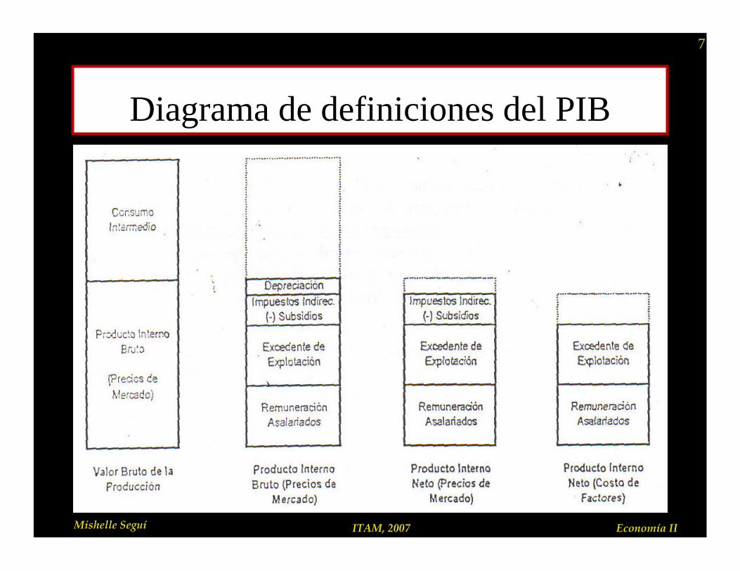
Diagrama de definiciones del PIB
8
Mishelle Seguí ITAM, 2007 Economía II
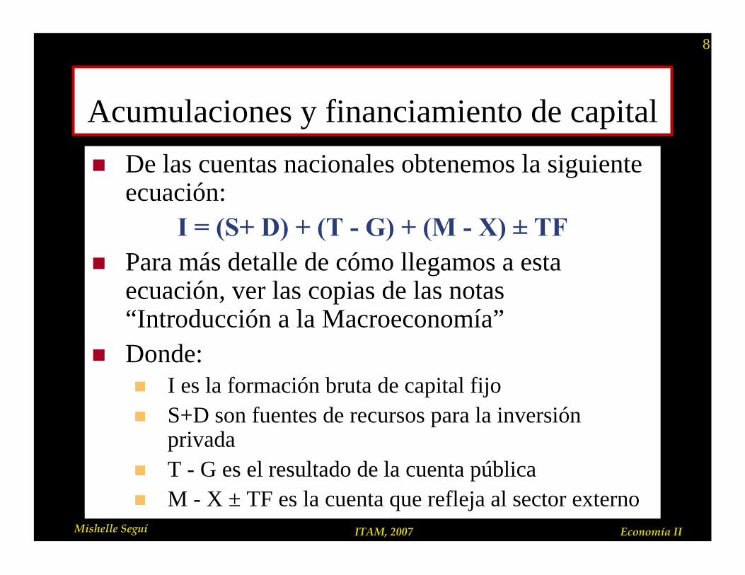
Acumulaciones y financiamiento de capital
n De las cuentas nacionales obtenemos la siguiente ecuación:
I = (S+ D) + (T - G) + (M - X) ± TFn Para más detalle de cómo llegamos a esta
ecuación, ver las copias de las notas “Introducción a la Macroeconomía”
n Donde:n I es la formación bruta de capital fijon S+D son fuentes de recursos para la inversión
privadan T - G es el resultado de la cuenta públican M - X ± TF es la cuenta que refleja al sector externo
9
Mishelle Seguí ITAM, 2007 Economía II
n Si T < G el gobierno presentará un déficitn Si T > G el gobierno presentará un superávit, ese ahorro
gubernamental puede utilizarse para favorecer lainversión.
n Si M ± TF > X la cuenta tendrá un déficit, por lo que elresto del mundo nos estará prestando capital.
n Si M ± TF < X México estará prestando al resto delmundo y la cuenta será superavitaria
n Cabe mencionar que invertir en el corto plazo es un gasto, un elemento de la demanda agregada, mientras que en el largo plazo la inversión crea recursos adicionales queaumentan la capacidad productiva generando oferta agregada.
10
Mishelle Seguí ITAM, 2007 Economía II
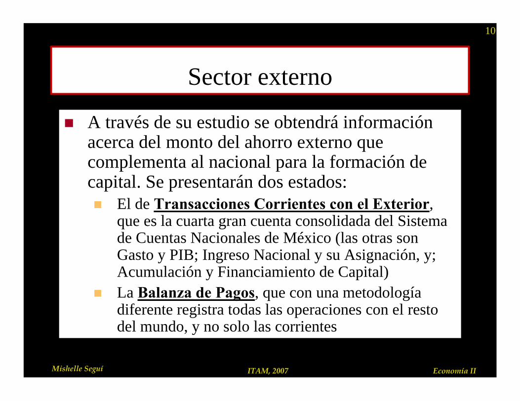
Sector externo
n A través de su estudio se obtendrá información acerca del monto del ahorro externo quecomplementa al nacional para la formación de capital. Se presentarán dos estados:n El de Transacciones Corrientes con el Exterior,
que es la cuarta gran cuenta consolidada del Sistemade Cuentas Nacionales de México (las otras son Gasto y PIB; Ingreso Nacional y su Asignación, y; Acumulación y Financiamiento de Capital)
n La Balanza de Pagos, que con una metodología diferente registra todas las operaciones con el restodel mundo, y no solo las corrientes
11
Mishelle Seguí ITAM, 2007 Economía II
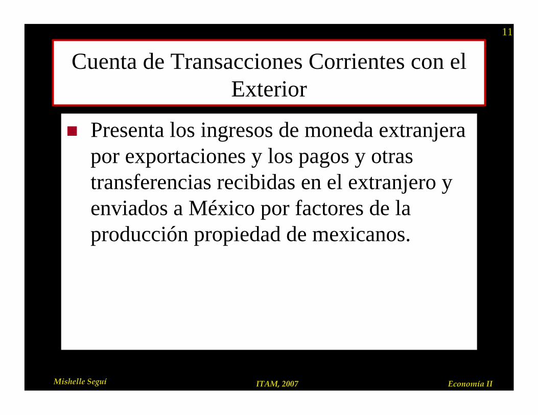
Cuenta de Transacciones Corrientes con el Exterior
n Presenta los ingresos de moneda extranjera por exportaciones y los pagos y otras transferencias recibidas en el extranjero yenviados a México por factores de laproducción propiedad de mexicanos.
12
Mishelle Seguí ITAM, 2007 Economía II
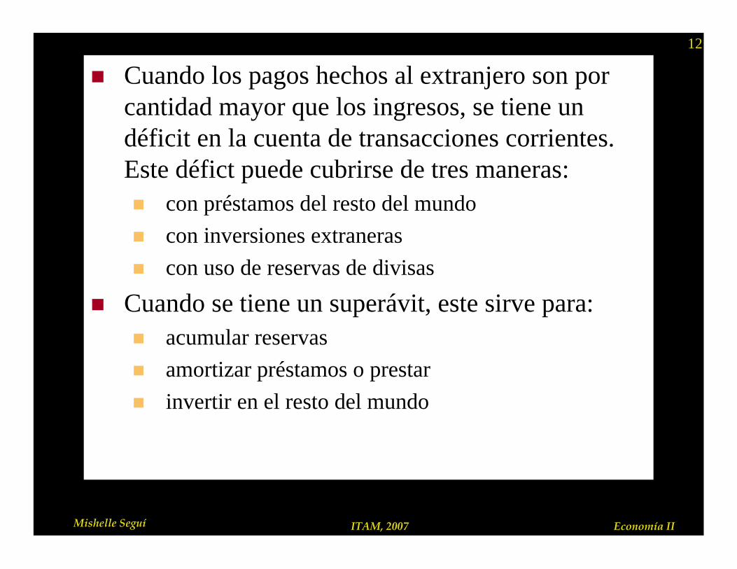
n Cuando los pagos hechos al extranjero son por cantidad mayor que los ingresos, se tiene un déficit en la cuenta de transacciones corrientes. Este défict puede cubrirse de tres maneras:n con préstamos del resto del mundo
n con inversiones extraneras
n con uso de reservas de divisas
n Cuando se tiene un superávit, este sirve para:n acumular reservas
n amortizar préstamos o prestar
n invertir en el resto del mundo
13
Mishelle Seguí ITAM, 2007 Economía II
n La cuenta de Transacciones Corrientes con el Exterior del Sistema de Cuentas Nacionales se relaciona estrechamente con el otro gran estado financiero que recoge las operaciones y transacciones realizadas entre la economía nacional y el resto del mundo
14
Mishelle Seguí ITAM, 2007 Economía II
Balanza de Pagos
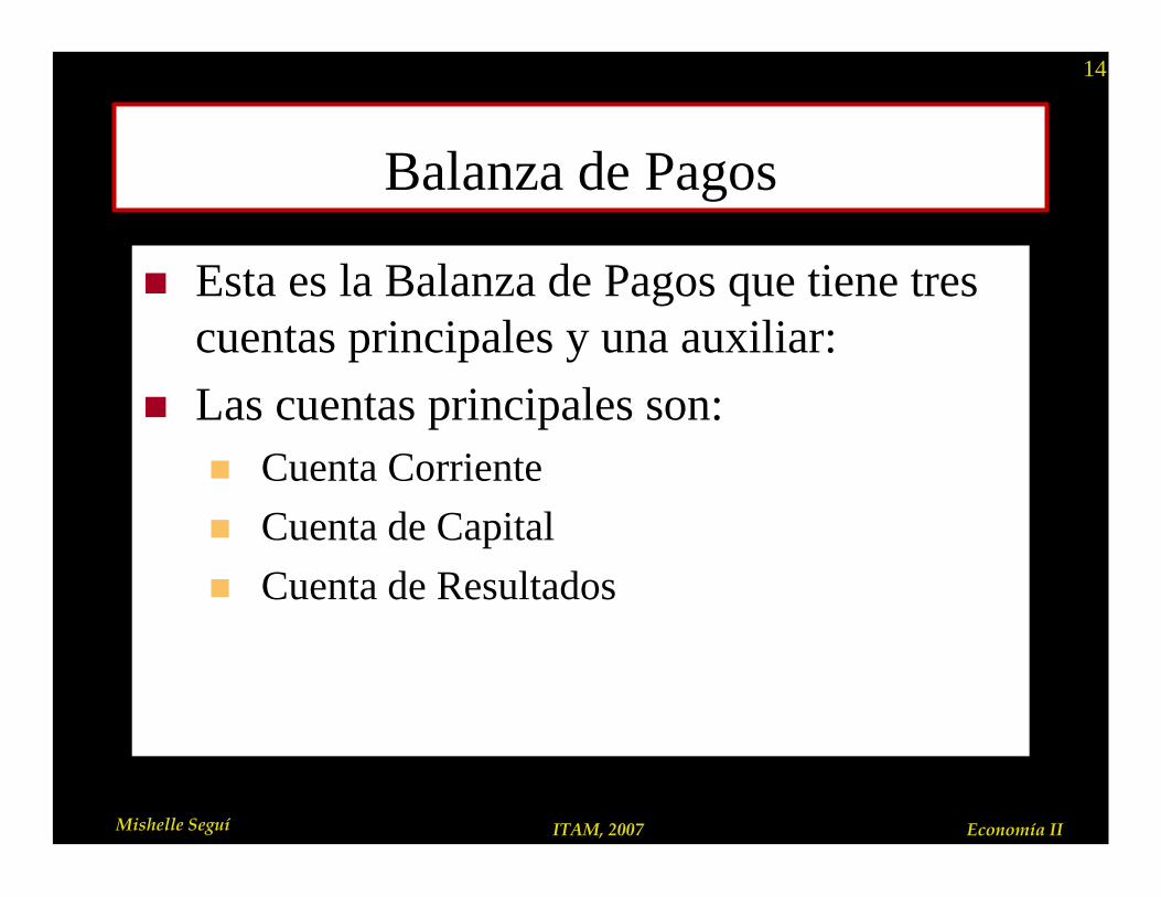
n Esta es la Balanza de Pagos que tiene tres cuentas principales y una auxiliar:
n Las cuentas principales son:n Cuenta Corriente
n Cuenta de Capital
n Cuenta de Resultados
15
Mishelle Seguí ITAM, 2007 Economía II
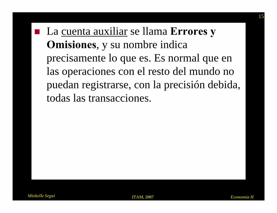
n La cuenta auxiliar se llama Errores yOmisiones, y su nombre indica precisamente lo que es. Es normal que enlas operaciones con el resto del mundo nopuedan registrarse, con la precisión debida,todas las transacciones.

16
Mishelle Seguí ITAM, 2007 Economía II
Cuenta Corriente
n Incluye todas las transacciones por venta ycompra de mercancías y servicios y por pagospor el uso de factores de producción domiciliados en el resto del mundo.
1. Ingresos. Los rubros principales son:n Exportaciones de mercancías.n Ingresos por transacciones fronterizas (o ventas en
ciudades fronterizas a residentes de otros países).n Servicios por transformación (maquila)n Pago a mexicanos en el extranjeron Turismo
17
Mishelle Seguí ITAM, 2007 Economía II
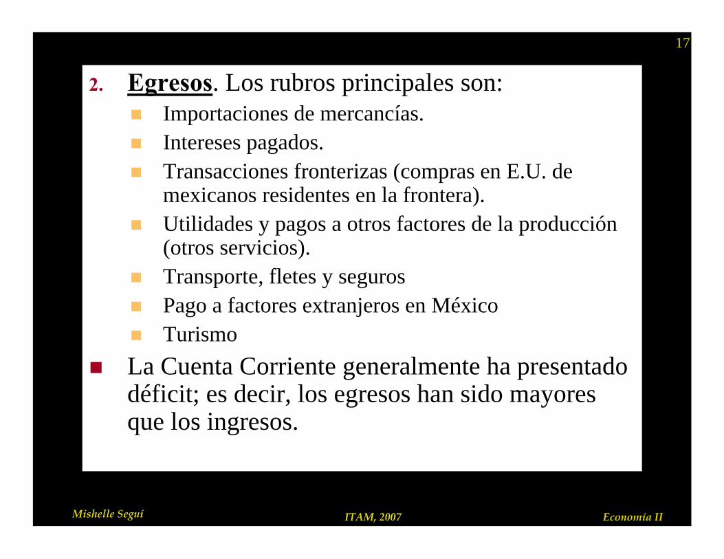
2. Egresos. Los rubros principales son:n Importaciones de mercancías.n Intereses pagados.n Transacciones fronterizas (compras en E.U. de
mexicanos residentes en la frontera).n Utilidades y pagos a otros factores de la producción
(otros servicios).n Transporte, fletes y segurosn Pago a factores extranjeros en Méxicon Turismo
n La Cuenta Corriente generalmente ha presentado déficit; es decir, los egresos han sido mayores que los ingresos.
18
Mishelle Seguí ITAM, 2007 Economía II
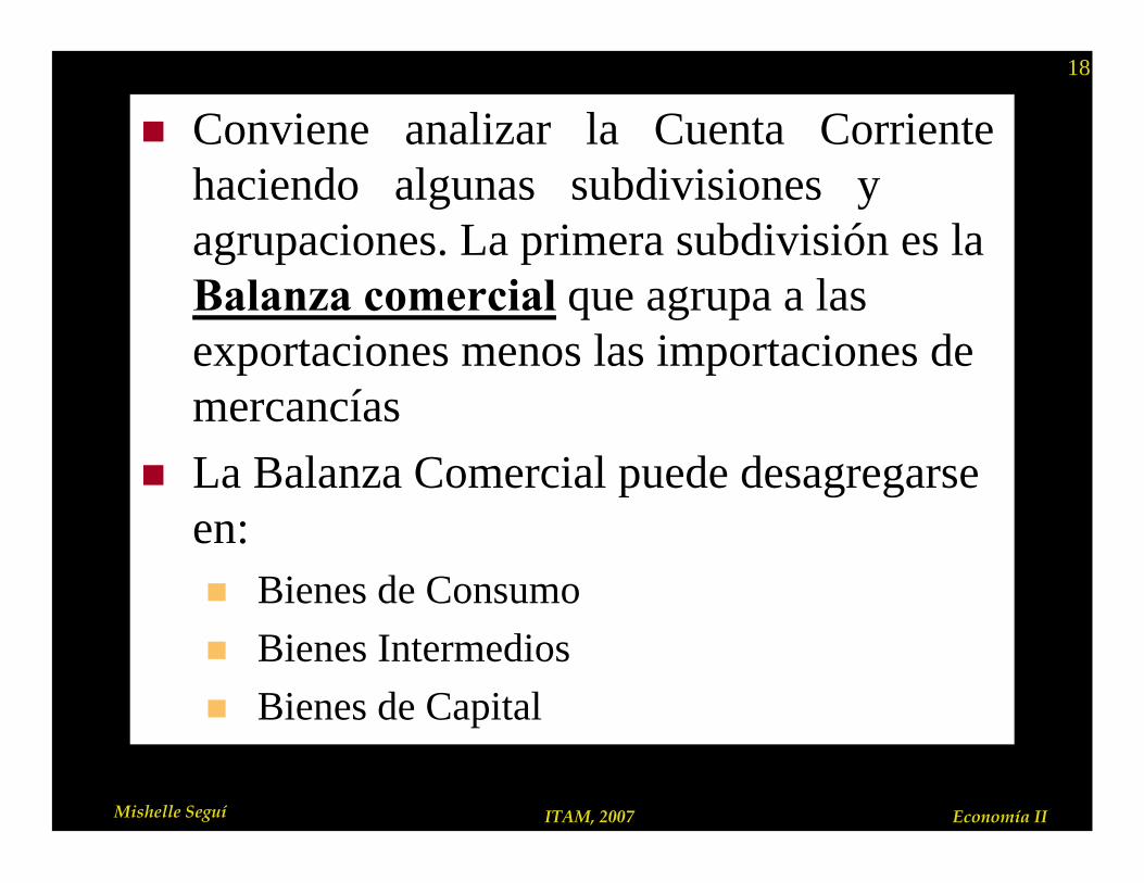
n Conviene analizar la Cuenta Corriente haciendo algunas subdivisiones yagrupaciones. La primera subdivisión es laBalanza comercial que agrupa a lasexportaciones menos las importaciones de mercancías
n La Balanza Comercial puede desagregarseen:n Bienes de Consumo
n Bienes Intermedios
n Bienes de Capital
19
Mishelle Seguí ITAM, 2007 Economía II
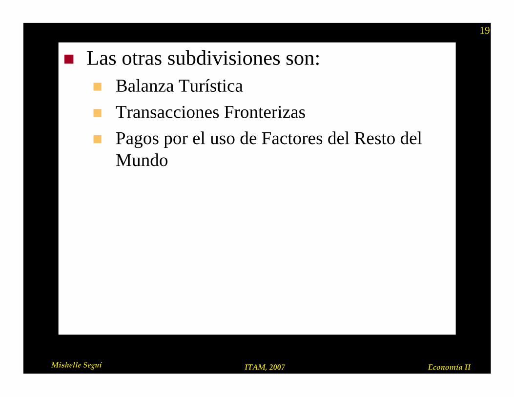
n Las otras subdivisiones son:n Balanza Turística
n Transacciones Fronterizas
n Pagos por el uso de Factores del Resto delMundo
20
Mishelle Seguí ITAM, 2007 Economía II
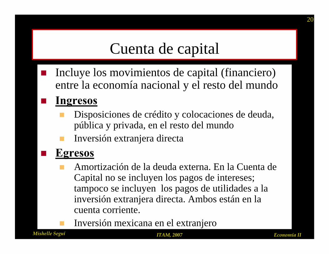
Cuenta de capitaln Incluye los movimientos de capital (financiero)
entre la economía nacional y el resto del mundon Ingresos
n Disposiciones de crédito y colocaciones de deuda,pública y privada, en el resto del mundo
n Inversión extranjera directa
n Egresosn Amortización de la deuda externa. En la Cuenta de
Capital no se incluyen los pagos de intereses; tampoco se incluyen los pagos de utilidades a la inversión extranjera directa. Ambos están en lacuenta corriente.
n Inversión mexicana en el extranjero
21
Mishelle Seguí ITAM, 2007 Economía II
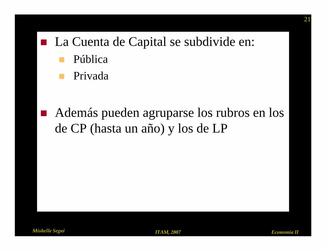
n La Cuenta de Capital se subdivide en:n Pública
n Privada
n Además pueden agruparse los rubros en los de CP (hasta un año) y los de LP
22
Mishelle Seguí ITAM, 2007 Economía II
Cuenta de Resultados
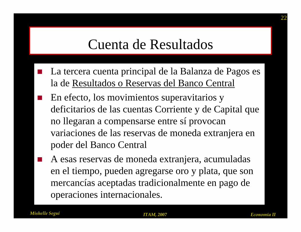
n La tercera cuenta principal de la Balanza de Pagos esla de Resultados o Reservas del Banco Central
n En efecto, los movimientos superavitarios ydeficitarios de las cuentas Corriente y de Capital queno llegaran a compensarse entre sí provocan variaciones de las reservas de moneda extranjera enpoder del Banco Central
n A esas reservas de moneda extranjera, acumuladasen el tiempo, pueden agregarse oro y plata, que sonmercancías aceptadas tradicionalmente en pago deoperaciones internacionales.
23
Mishelle Seguí ITAM, 2007 Economía II
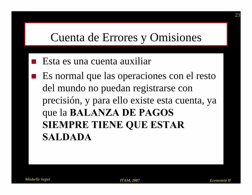
Cuenta de Errores y Omisiones
n Esta es una cuenta auxiliar
n Es normal que las operaciones con el restodel mundo no puedan registrarse conprecisión, y para ello existe esta cuenta, ya que la BALANZA DE PAGOS SIEMPRE TIENE QUE ESTAR SALDADA

24
Mishelle Seguí ITAM, 2007 Economía II
n En resumen:
Variación de la Reserva=Resultados de la CC+Resultado de la CK+CR+EyO
25
Mishelle Seguí ITAM, 2007 Economía II
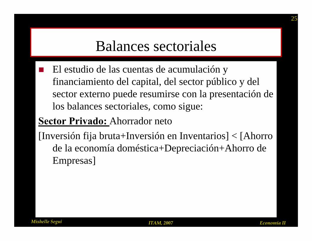
Balances sectoriales
n El estudio de las cuentas de acumulación yfinanciamiento del capital, del sector público y del sector externo puede resumirse con la presentación delos balances sectoriales, como sigue:
Sector Privado: Ahorrador neto
[Inversión fija bruta+Inversión en Inventarios] < [Ahorro de la economía doméstica+Depreciación+Ahorro de Empresas]
26
Mishelle Seguí ITAM, 2007 Economía II
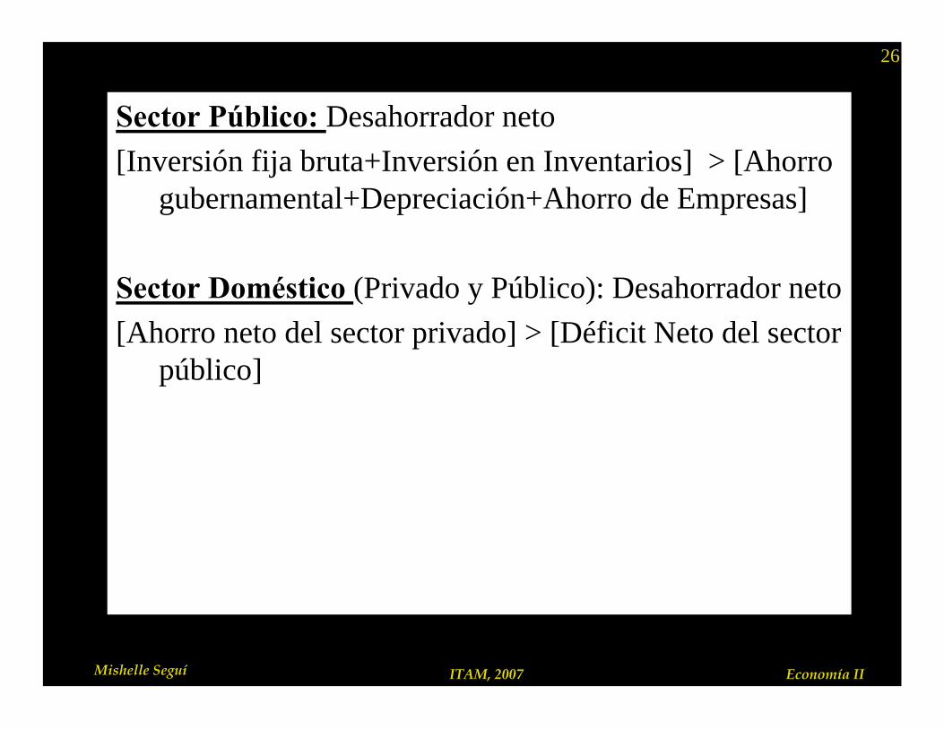
Sector Público: Desahorrador neto
[Inversión fija bruta+Inversión en Inventarios] > [Ahorro gubernamental+Depreciación+Ahorro de Empresas]
Sector Doméstico (Privado y Público): Desahorrador neto
[Ahorro neto del sector privado] > [Déficit Neto del sector público]
27
Mishelle Seguí ITAM, 2007 Economía II
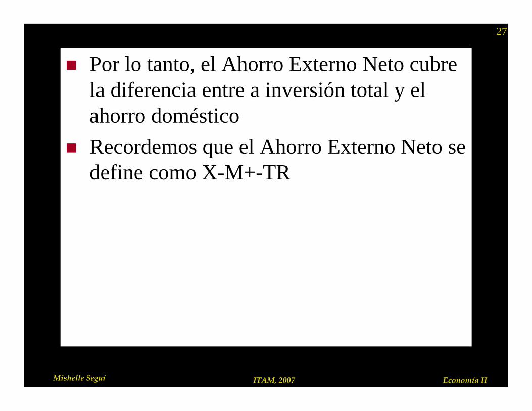
n Por lo tanto, el Ahorro Externo Neto cubre la diferencia entre a inversión total y el ahorro doméstico
n Recordemos que el Ahorro Externo Neto se define como X-M+-TR
28
Mishelle Seguí ITAM, 2007 Economía II
El modelo de Solow
n El siguiente resumen es de las presentaciones de Mankiw, que ustedes tienen el Comunidad bajo Materiales del Departamente

29
Mishelle Seguí ITAM, 2007 Economía II
The Solow Modeln due to Robert Solow,
won Nobel Prize for contributions to the study of economic growth
n a major paradigm:n widely used in policy makingn benchmark against which most
recent growth theories are compared
n looks at the determinants of economic growth and the standard of living in the long run

30
Mishelle Seguí ITAM, 2007 Economía II
The production function
n In aggregate terms: Y = F (K, L )
n Define: y = Y/L = output per worker k = K/L = capital per worker
n Assume constant returns to scale:zY = F (zK, zL ) for any z > 0
n Pick z = 1/L. Then Y/L = F (K/L , 1)
y = F (k, 1)
y = f(k) where f(k) = F (k, 1)

31
Mishelle Seguí ITAM, 2007 Economía II
The production functionOutput per worker, y
Capital per worker, k
f(k)
Note: this production function exhibits diminishing MPK. Note: this production function exhibits diminishing MPK.
1MPK =f(k +1) – f(k)
32
Mishelle Seguí ITAM, 2007 Economía II
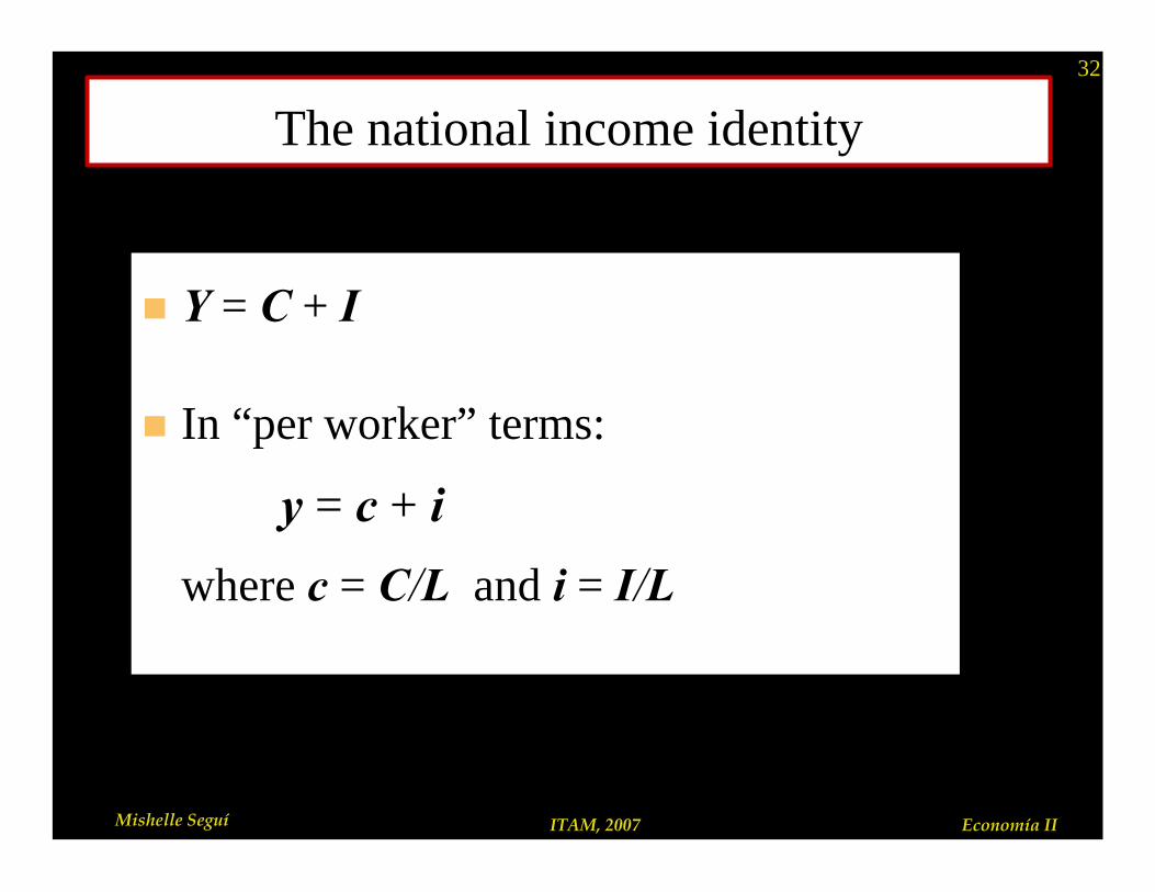
The national income identity
n Y = C + I
n In “per worker” terms:
y = c + i
where c = C/L and i = I/L
33
Mishelle Seguí ITAM, 2007 Economía II
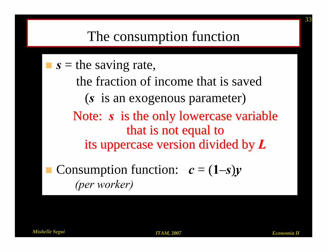
The consumption function
n s = the saving rate, the fraction of income that is saved
(s is an exogenous parameter)Note: Note: ss is the only lowercase variable is the only lowercase variable
that is not equal to that is not equal to its uppercase version divided by its uppercase version divided by LL
n Consumption function: c = (1–s)y(per worker)
34
Mishelle Seguí ITAM, 2007 Economía II
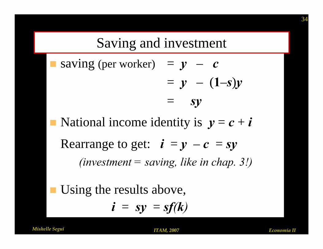
Saving and investmentn saving (per worker) = y – c
= y – (1–s)y
= sy
n National income identity is y = c + i
Rearrange to get: i = y – c = sy(investment = saving, like in chap. 3!)
n Using the results above, i = sy = sf(k)

35
Mishelle Seguí ITAM, 2007 Economía II
Output, consumption, and investment
Output per worker, y
Capital per worker, k
f(k)
sf (k)
k1
y1
i1
c1
36
Mishelle Seguí ITAM, 2007 Economía II
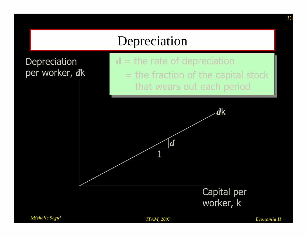
Depreciation
Depreciation per worker, δδk
Capital per worker, k
δδk
δδ = the rate of depreciation = the fraction of the capital stock
that wears out each period
δδ = the rate of depreciation = the fraction of the capital stock
that wears out each period
1δδ
37
Mishelle Seguí ITAM, 2007 Economía II
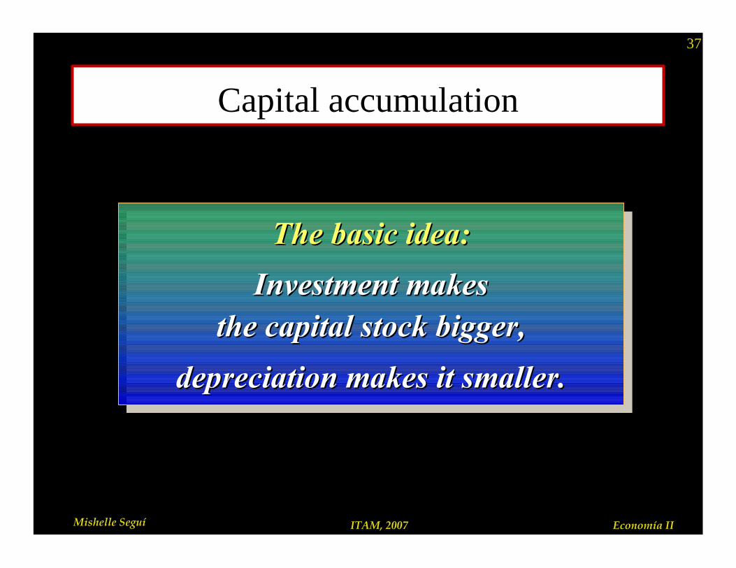
Capital accumulation
The basic idea:
Investment makes the capital stock bigger,
depreciation makes it smaller.
The basic idea:The basic idea:
Investment makes Investment makes the capital stock bigger,the capital stock bigger,
depreciation makes it smaller.depreciation makes it smaller.
38
Mishelle Seguí ITAM, 2007 Economía II
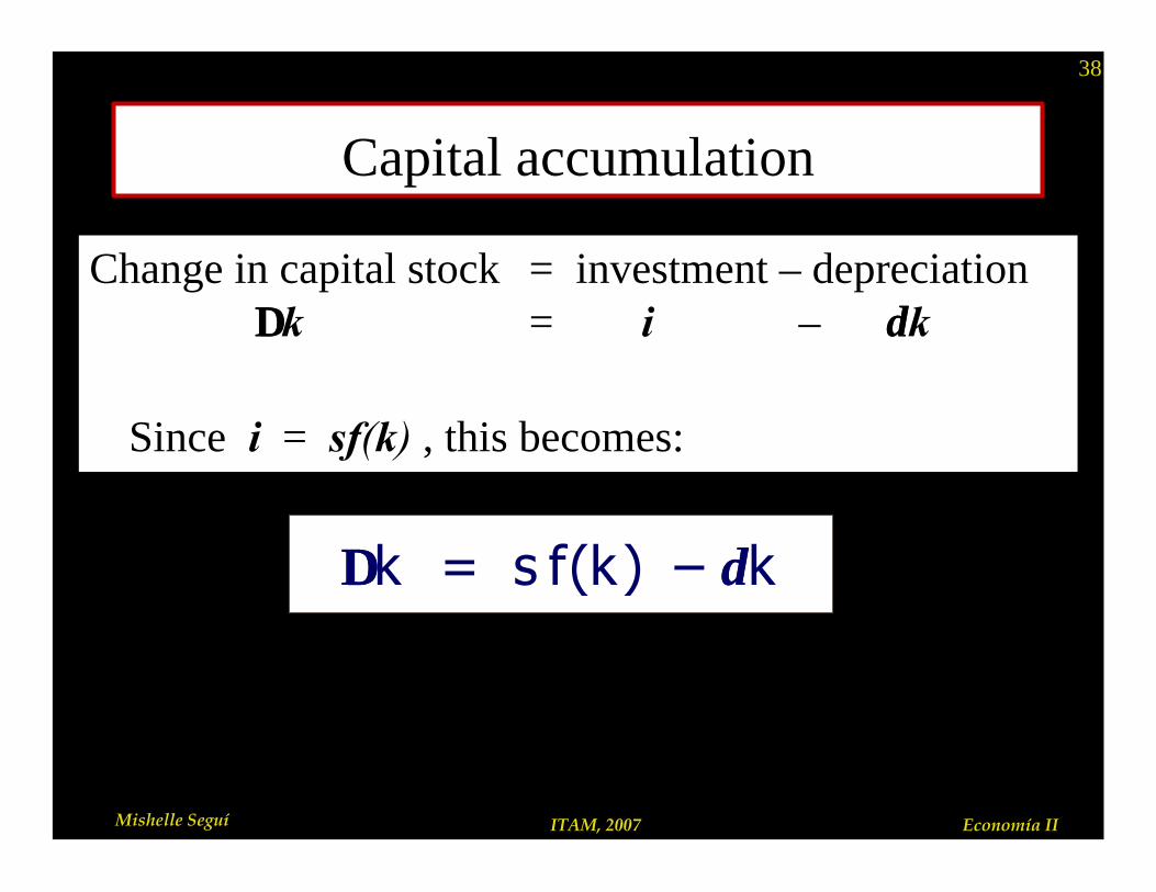
Capital accumulation
Change in capital stock = investment – depreciation∆∆k = i – δδk
Since i = sf(k) , this becomes:
∆∆k = s f(k) – δδk
39
Mishelle Seguí ITAM, 2007 Economía II
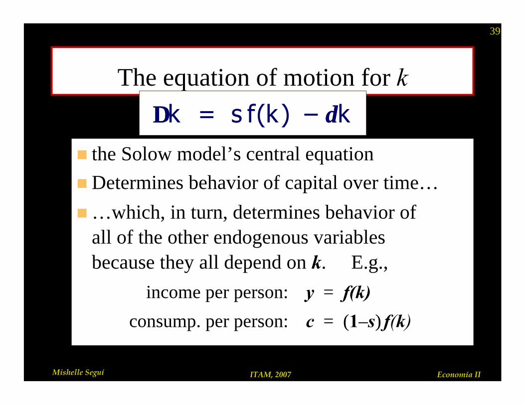
The equation of motion for k
n the Solow model’s central equation
nDetermines behavior of capital over time…
n…which, in turn, determines behavior of all of the other endogenous variables because they all depend on k. E.g.,
income per person: y = f(k)
consump. per person: c = (1–s) f(k)
∆∆k = s f(k) – δδk

40
Mishelle Seguí ITAM, 2007 Economía II
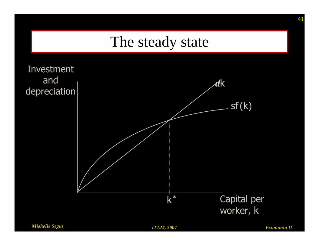
The steady state
If investment is just enough to cover depreciation [sf(k) = δδk ],
then capital per worker will remain constant: ∆∆k = 0.
This constant value, denoted k*, is called the steady state capital stock.
∆∆k = s f(k) – δδk
41
Mishelle Seguí ITAM, 2007 Economía II
The steady state
Investment and
depreciation
Capital per worker, k
sf (k)
δδk
k*
42
Mishelle Seguí ITAM, 2007 Economía II
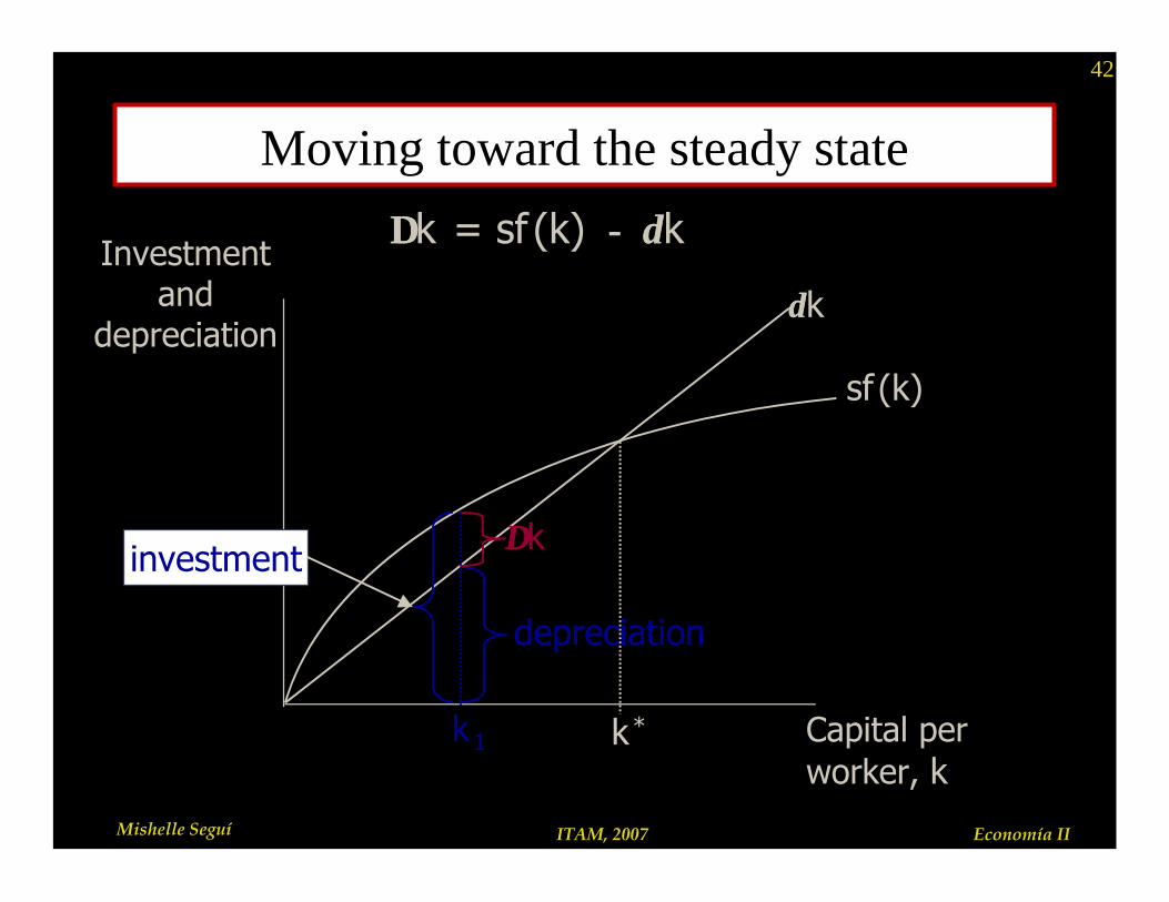
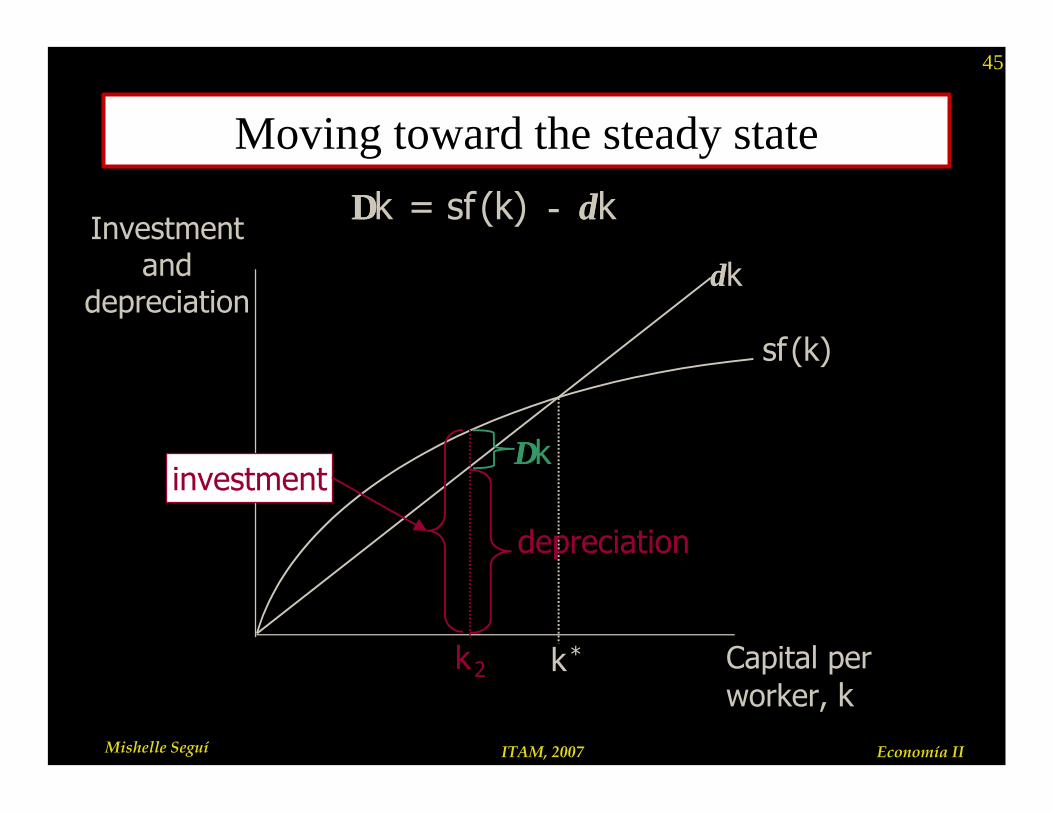
Moving toward the steady state
Investment and
depreciation
Capital per worker, k
sf (k)
δδk
k*
∆∆k = sf (k) −− δδk
depreciation
∆∆k
k1
investment
43
Mishelle Seguí ITAM, 2007 Economía II
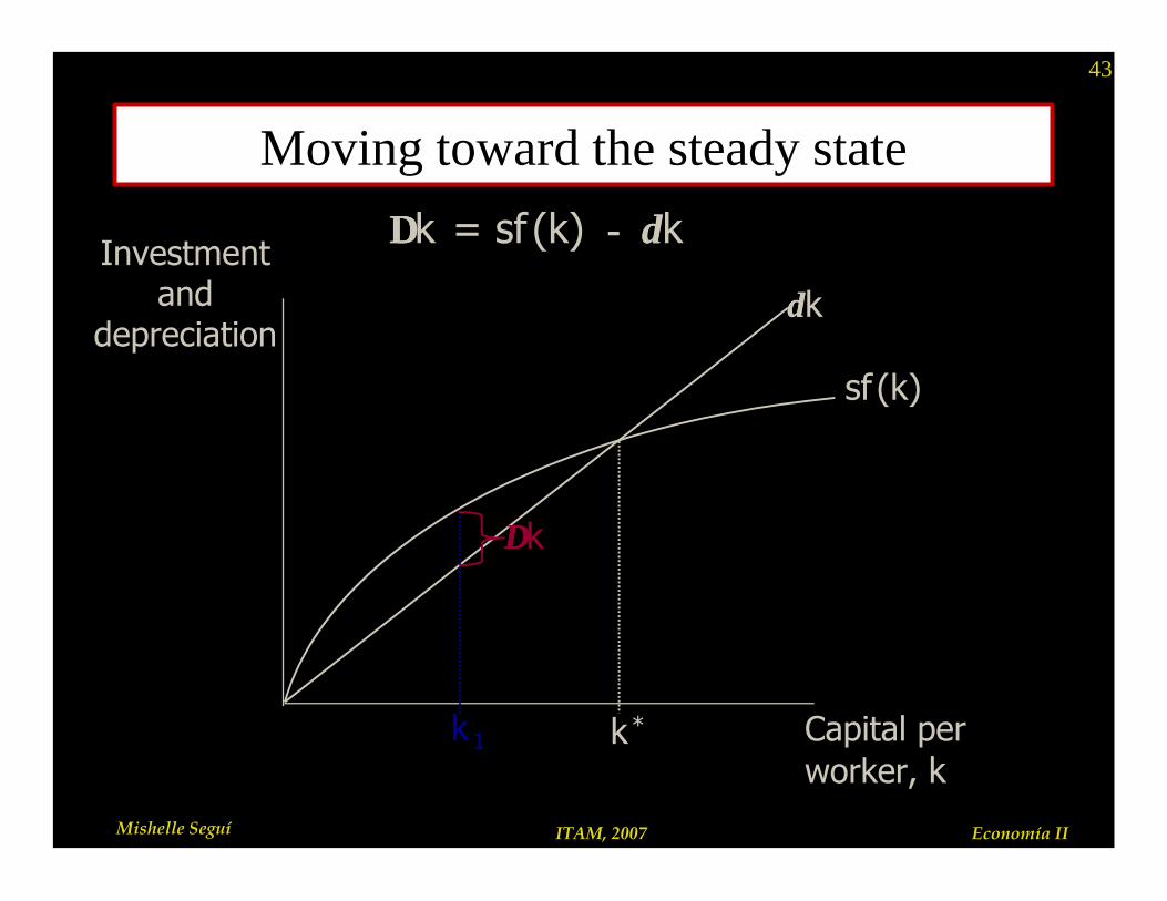
Moving toward the steady state
Investment and
depreciation
Capital per worker, k
sf (k)
δδk
k*k1
∆∆k = sf (k) −− δδk
∆∆k
44
Mishelle Seguí ITAM, 2007 Economía II
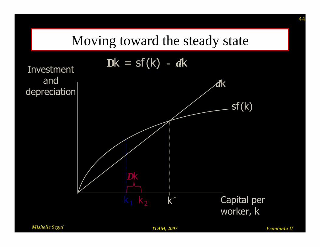
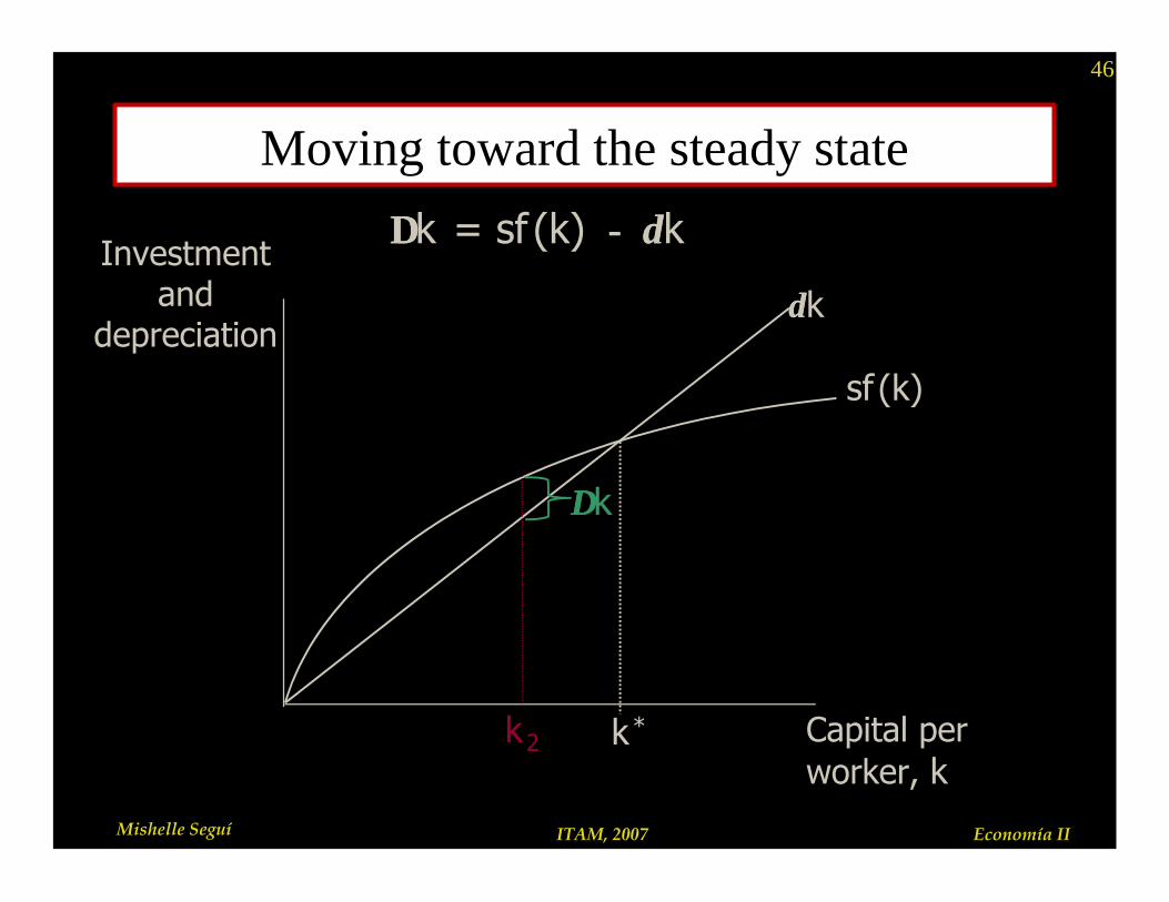
Moving toward the steady state
Investment and
depreciation
Capital per worker, k
sf (k)
δδk
k*k1
∆∆k = sf (k) −− δδk
∆∆k
k2
45
Mishelle Seguí ITAM, 2007 Economía II
Moving toward the steady state
Investment and
depreciation
Capital per worker, k
sf (k)
δδk
k*
∆∆k = sf (k) −− δδk
k2
investment
depreciation
∆∆k
46
Mishelle Seguí ITAM, 2007 Economía II
Moving toward the steady state
Investment and
depreciation
Capital per worker, k
sf (k)
δδk
k*
∆∆k = sf (k) −− δδk
∆∆k
k2
47
Mishelle Seguí ITAM, 2007 Economía II
Moving toward the steady state
Investment and
depreciation
Capital per worker, k
sf (k)
δδk
k*
∆∆k = sf (k) −− δδk
k2
∆∆k
k3
48
Mishelle Seguí ITAM, 2007 Economía II
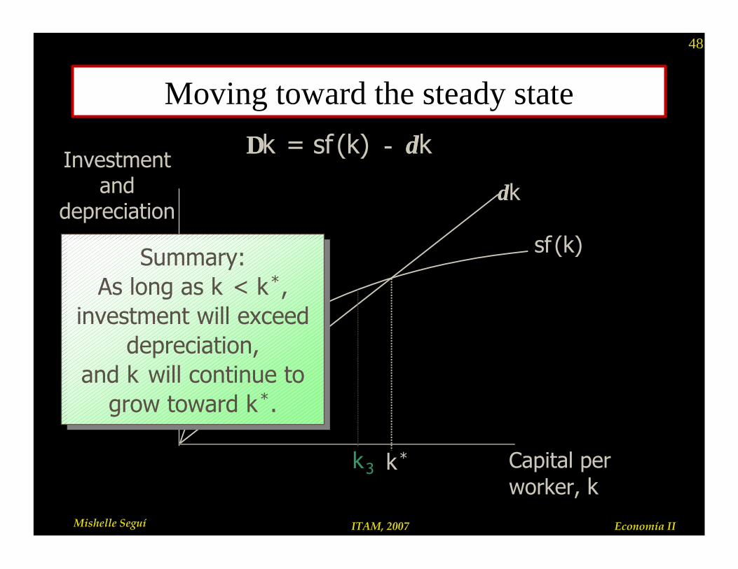
Moving toward the steady state
Investment and
depreciation
Capital per worker, k
sf (k)
δδk
k*
∆∆k = sf (k) −− δδk
k3
Summary:As long as k < k*,
investment will exceed depreciation,
and k will continue to grow toward k*.
Summary:As long as k < k*,
investment will exceed depreciation,
and k will continue to grow toward k*.
49
Mishelle Seguí ITAM, 2007 Economía II
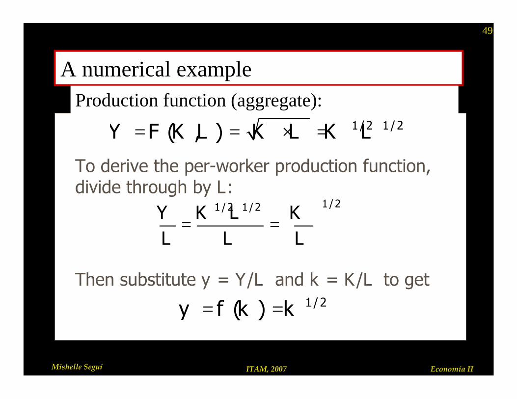
A numerical exampleProduction function (aggregate):
= = × = 1 /2 1 /2( , )Y F K L K L K L
= =
1 /21 / 2 1 /2Y K L KL L L
= = 1 /2( )y f k k
To derive the per-worker production function, divide through by L:
Then substitute y = Y/L and k = K/L to get

50
Mishelle Seguí ITAM, 2007 Economía II
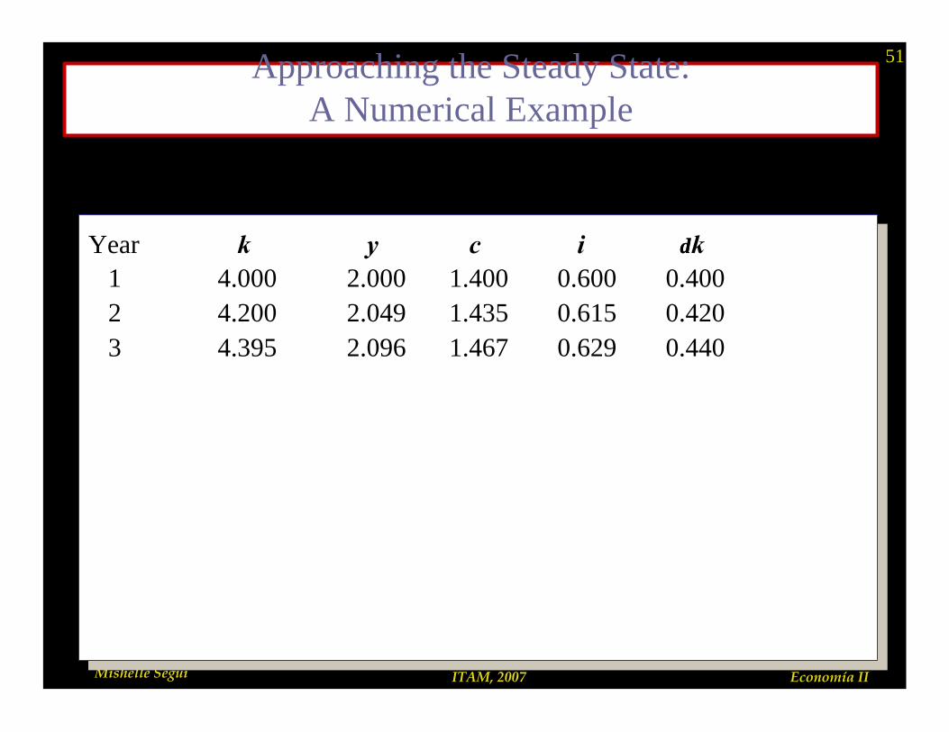
A numerical example, cont.
Assume:
n s = 0.3
n δδ = 0.1
n initial value of k = 4.0
51
Mishelle Seguí ITAM, 2007 Economía II
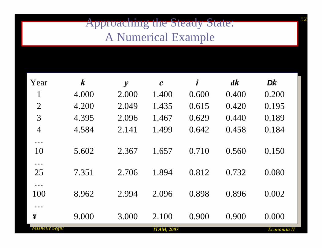
Approaching the Steady State: A Numerical Example
Year k y c i δδk1 4.000 2.000 1.400 0.600 0.4002 4.200 2.049 1.435 0.615 0.4203 4.395 2.096 1.467 0.629 0.440
Year k y c i δδk1 4.000 2.000 1.400 0.600 0.4002 4.200 2.049 1.435 0.615 0.4203 4.395 2.096 1.467 0.629 0.440
Assumptions: ; 0.3; 0.1; initial 4.0y k s kδ= = = =
52
Mishelle Seguí ITAM, 2007 Economía II
Approaching the Steady State: A Numerical Example
Year k y c i δδk Dk1 4.000 2.000 1.400 0.600 0.400 0.2002 4.200 2.049 1.435 0.615 0.420 0.1953 4.395 2.096 1.467 0.629 0.440 0.1894 4.584 2.141 1.499 0.642 0.458 0.184
…10 5.602 2.367 1.657 0.710 0.560 0.150…25 7.351 2.706 1.894 0.812 0.732 0.080…
100 8.962 2.994 2.096 0.898 0.896 0.002…∞∞ 9.000 3.000 2.100 0.900 0.900 0.000
Assumptions: ; 0.3; 0.1; initial 4.0y k s kδ= = = =
53
Mishelle Seguí ITAM, 2007 Economía II
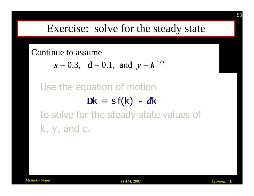
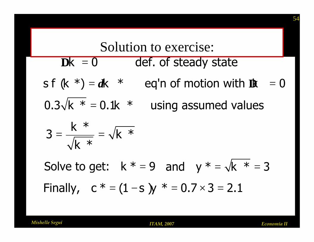
Exercise: solve for the steady state
Continue to assume s = 0.3, δδ = 0.1, and y = k 1/2
Use the equation of motion ∆∆k = s f(k) −− δδk
to solve for the steady-state values of k, y, and c.
54
Mishelle Seguí ITAM, 2007 Economía II
Solution to exercise:0 def. of steady statek∆∆ =
and * * 3y k= =
( *) * eq'n of motion with 0s f k k k= =δδ ∆∆
0.3 * 0.1 * using assumed valuesk k=
*3 *
*
kk
k= =
Solve to get: * 9k =
Finally, * (1 ) * 0.7 3 2.1c s y= − = × =
55
Mishelle Seguí ITAM, 2007 Economía II
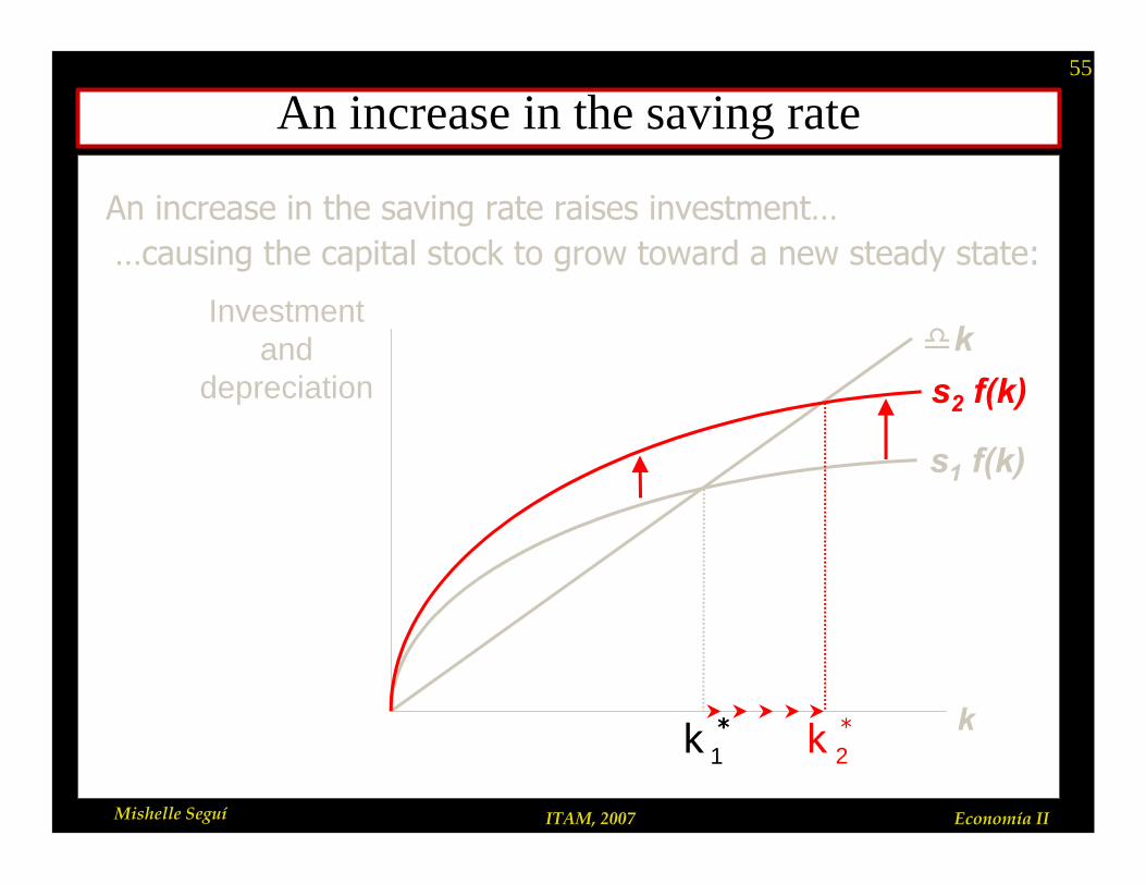
An increase in the saving rate
Investment and
depreciation
k
dk
s1 f(k)
*k 1
An increase in the saving rate raises investment……causing the capital stock to grow toward a new steady state:
s2 f(k)
*k 2
56
Mishelle Seguí ITAM, 2007 Economía II
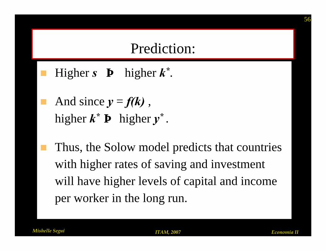
Prediction:
n Higher s ⇒⇒ higher k*.
n And since y = f(k) , higher k* ⇒⇒ higher y* .
n Thus, the Solow model predicts that countries with higher rates of saving and investment will have higher levels of capital and income per worker in the long run.
57
Mishelle Seguí ITAM, 2007 Economía II
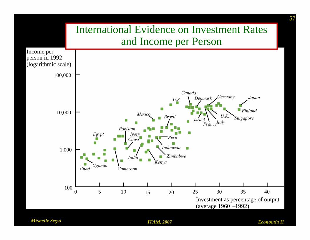
Egypt
Chad
Pakistan
Indonesia
ZimbabweKenya
India
CameroonUganda
Mexico
IvoryCoast
Brazil
Peru
U.K.
U.S.
Canada
FranceIsrael
GermanyDenmark
ItalySingapore
Japan
Finland
100,000
10,000
1,000
100
Income per person in 1992(logarithmic scale)
0 5 10 15Investment as percentage of output (average 1960 –1992)
20 25 30 35 40
International Evidence on Investment Rates and Income per Person
58
Mishelle Seguí ITAM, 2007 Economía II
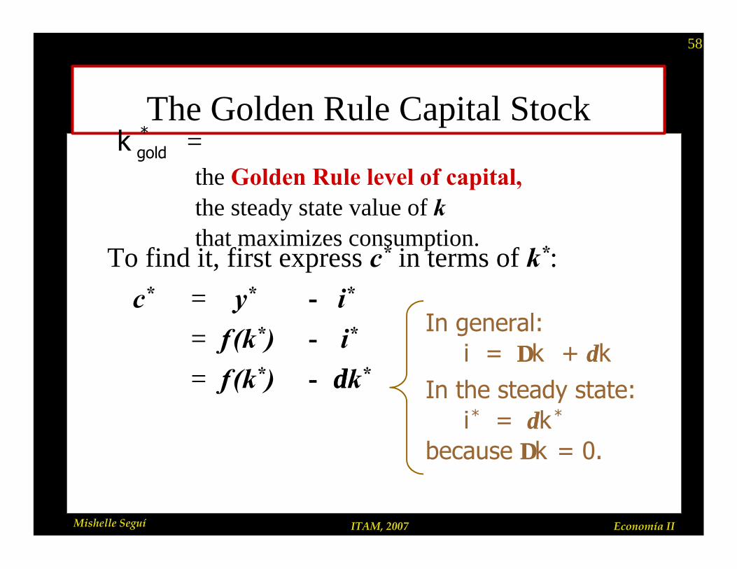
The Golden Rule Capital Stock
the Golden Rule level of capital,the steady state value of kthat maximizes consumption.
*goldk =
To find it, first express c* in terms of k*:
c* = y* −− i*
= f (k*) −− i*
= f (k*) −− δδk*
In general: i = ∆∆k + δδk
In the steady state:i* = δδk*
because ∆∆k = 0.

59
Mishelle Seguí ITAM, 2007 Economía II
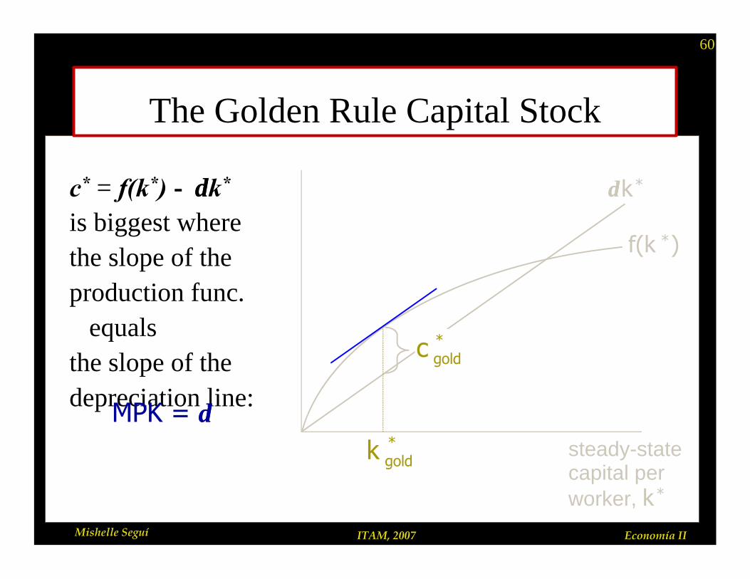
Then, graph f(k*) and δδk*, and look for the point where the gap between them is biggest.
The Golden Rule Capital Stocksteady state output and
depreciation
steady-state capital per worker, k*
f(k *)
δδk*
*goldk
*goldc
* *gold goldi kδ=
* *( )gold goldy f k=
60
Mishelle Seguí ITAM, 2007 Economía II
The Golden Rule Capital Stock
c* = f(k*) −− δδk*
is biggest where the slope of the production func.
equals the slope of the depreciation line:
steady-state capital per worker, k*
f(k *)
δδk*
*goldk
*goldc
MPK = δδ

61
Mishelle Seguí ITAM, 2007 Economía II
The transition to the Golden Rule Steady State
n The economy does NOT have a tendency to move toward the Golden Rule steady state.
n Achieving the Golden Rule requires that policymakers adjust s.
n This adjustment leads to a new steady state with higher consumption.
n But what happens to consumption during the transition to the Golden Rule?
62
Mishelle Seguí ITAM, 2007 Economía II
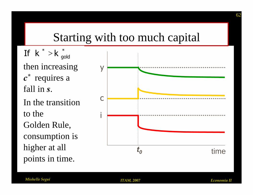
Starting with too much capital
then increasing c* requires a fall in s.
In the transition to the Golden Rule, consumption is higher at all points in time.
* *If goldk k>
timet0
c
i
y

63
Mishelle Seguí ITAM, 2007 Economía II
Starting with too little capital
then increasing c*
requires an increase in s.
Future generations enjoy higher consumption, but the current one experiences an initial drop in consumption.
* *If goldk k<
timet0
c
i
y
64
Mishelle Seguí ITAM, 2007 Economía II
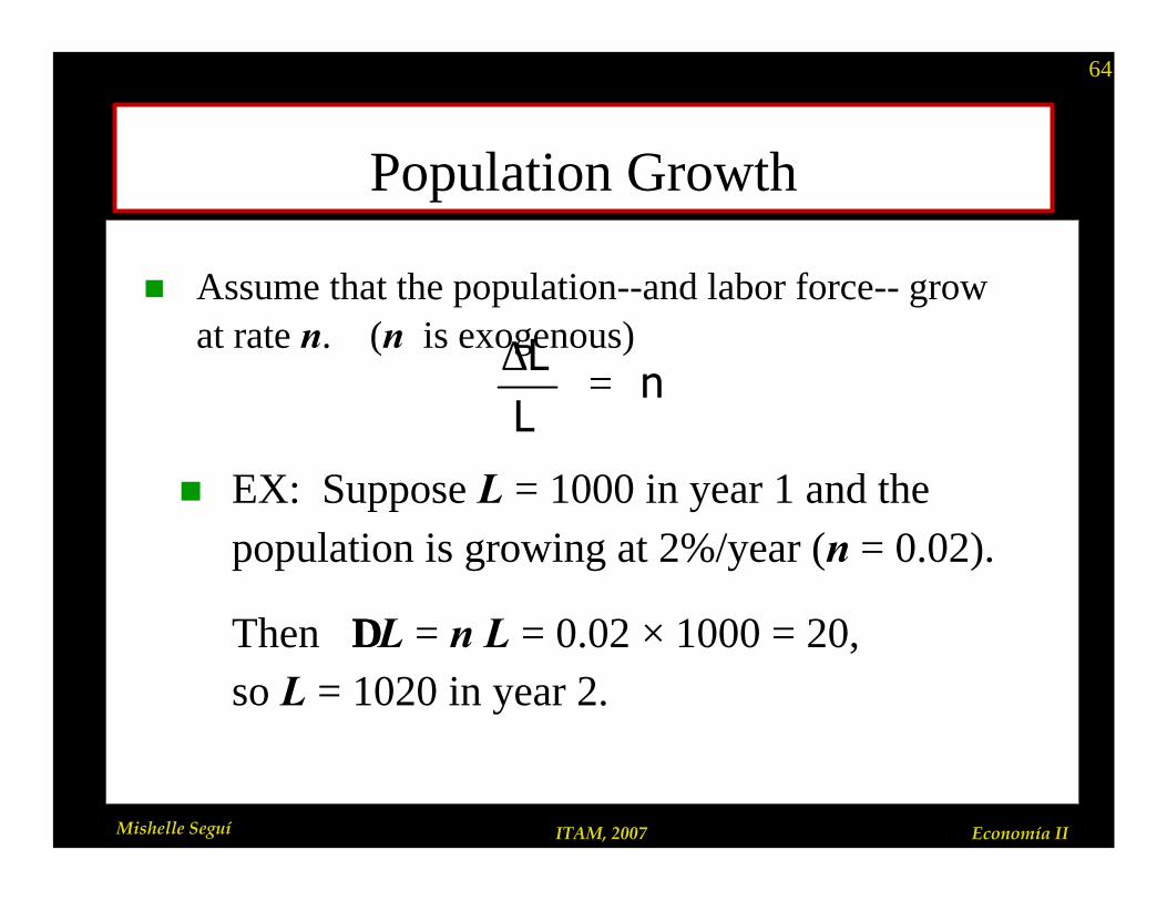
Population Growth
n Assume that the population--and labor force-- grow at rate n. (n is exogenous)L
nL
∆=
n EX: Suppose L = 1000 in year 1 and the population is growing at 2%/year (n = 0.02).
Then ∆∆L = n L = 0.02 × 1000 = 20,so L = 1020 in year 2.
65
Mishelle Seguí ITAM, 2007 Economía II
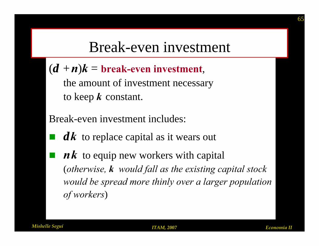
Break-even investment(δδ +n)k = break-even investment,
the amount of investment necessary to keep k constant.
Break-even investment includes:
n δδk to replace capital as it wears out
n nk to equip new workers with capital(otherwise, k would fall as the existing capital stock would be spread more thinly over a larger population of workers)
66
Mishelle Seguí ITAM, 2007 Economía II
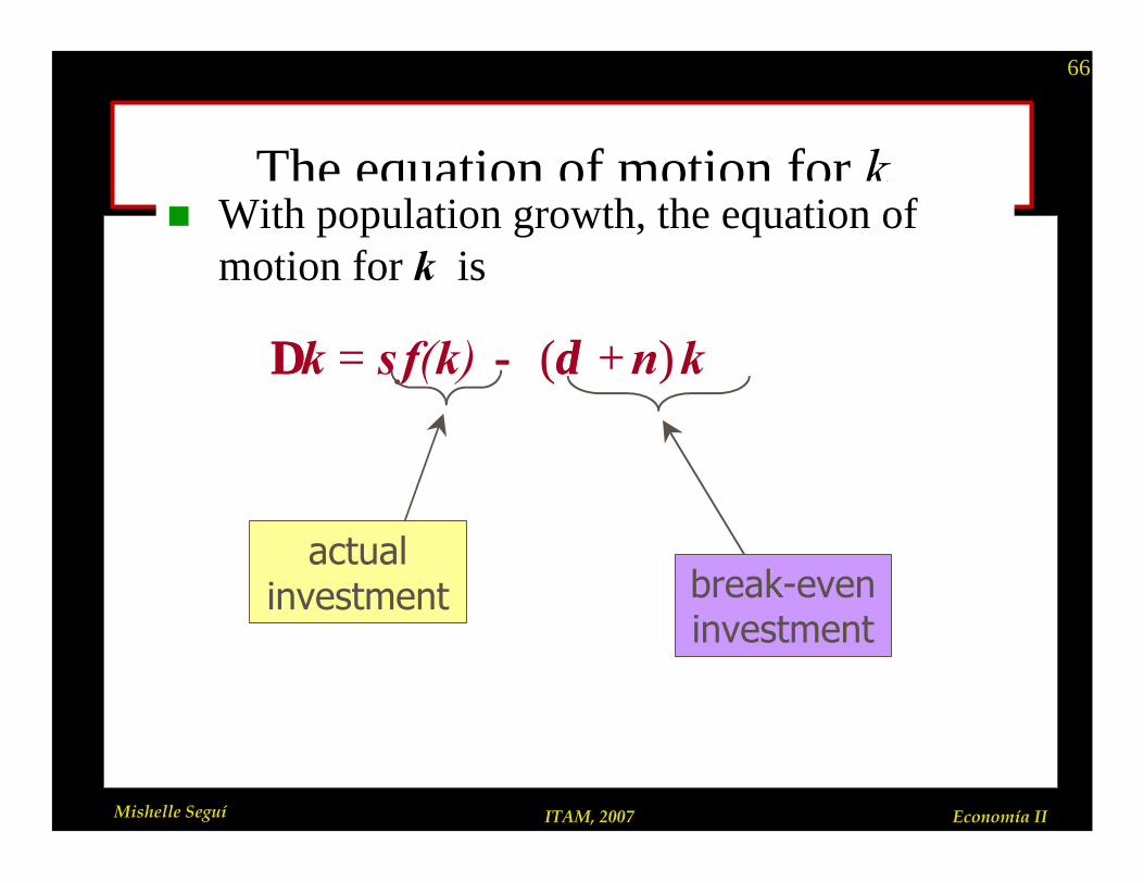
The equation of motion for kn With population growth, the equation of
motion for k is
∆∆k = s f(k) −− (δδ +n)k
break-even investment
actual investment
67
Mishelle Seguí ITAM, 2007 Economía II
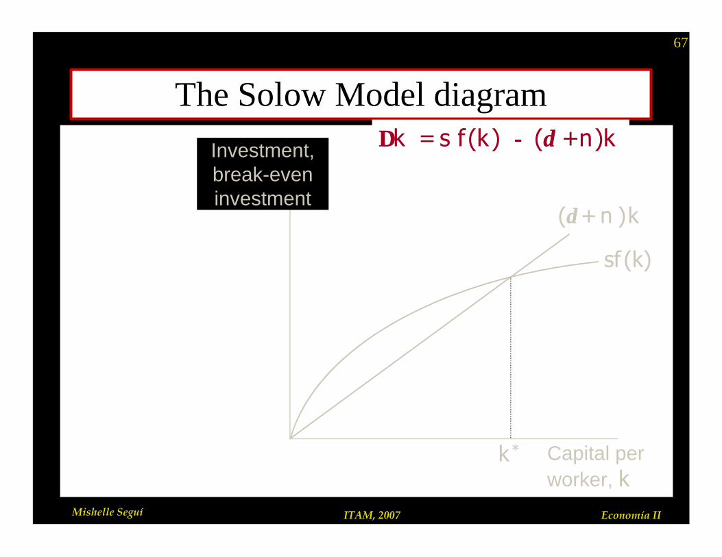
The Solow Model diagram
Investment, break-even investment
Capital per worker, k
sf (k)
(δδ + n )k
k*
∆∆k = s f(k) −− (δδ +n)k

68
Mishelle Seguí ITAM, 2007 Economía II
Tech. progress in the Solow model
n We now write the production function as:
n where L × E = the number of effective workers. n Hence, increases in labor efficiency have
the same effect on output as increases in the labor force.
( , )Y F K L E= ×
69
Mishelle Seguí ITAM, 2007 Economía II
Tech. progress in the Solow model
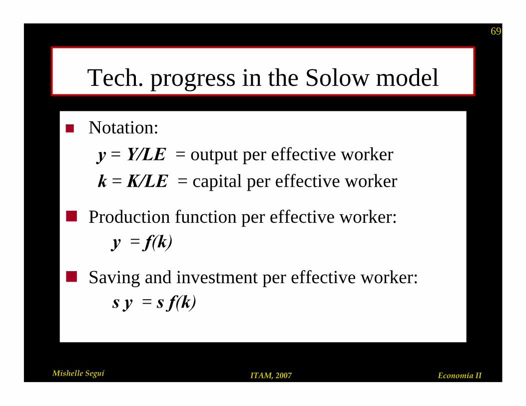
n Notation:
y = Y/LE = output per effective worker
k = K/LE = capital per effective worker
n Production function per effective worker:y = f(k)
n Saving and investment per effective worker:s y = s f(k)
70
Mishelle Seguí ITAM, 2007 Economía II
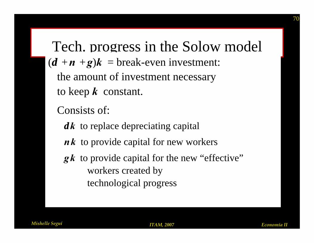
Tech. progress in the Solow model(δδ +n +g)k = break-even investment:
the amount of investment necessary to keep k constant.
Consists of:δδ k to replace depreciating capital
nk to provide capital for new workers
gk to provide capital for the new “effective” workers created by technological progress
71
Mishelle Seguí ITAM, 2007 Economía II
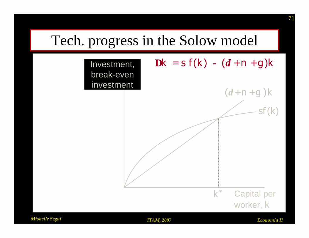
Tech. progress in the Solow model
Investment, break-even investment
Capital per worker, k
sf (k)
(δδ +n +g )k
k*
∆∆k = s f(k) −− (δδ +n +g)k
72
Mishelle Seguí ITAM, 2007 Economía II
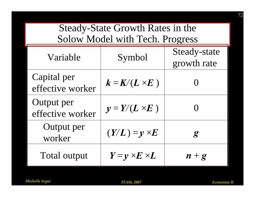
Steady-State Growth Rates in the Solow Model with Tech. Progress
n + gY =y ×E ×L Total output
g(Y/ L ) =y ×E Output per worker
0y =Y/ (L ×E )Output per effective worker
0k =K/ (L ×E )Capital per effective worker
Steady-state growth rate
SymbolVariable

73
Mishelle Seguí ITAM, 2007 Economía II
The Golden RuleTo find the Golden Rule capital stock, express c* in terms of k*:
c* = y* −− i*
= f (k*) −− (δδ +n +g)k*
c* is maximized when MPK = δδ + n + g
or equivalently, MPK − δδ = n + g
In the Golden Rule Steady State,
the marginal product of capital
net of depreciation equals the
pop. growth rate plus the rate of tech progress.
In the Golden In the Golden Rule Steady State, Rule Steady State,
the marginal the marginal product of capital product of capital
net of depreciation net of depreciation equals the equals the
pop. growth rate pop. growth rate plus the rate of plus the rate of tech progress.tech progress.
74
Mishelle Seguí ITAM, 2007 Economía II
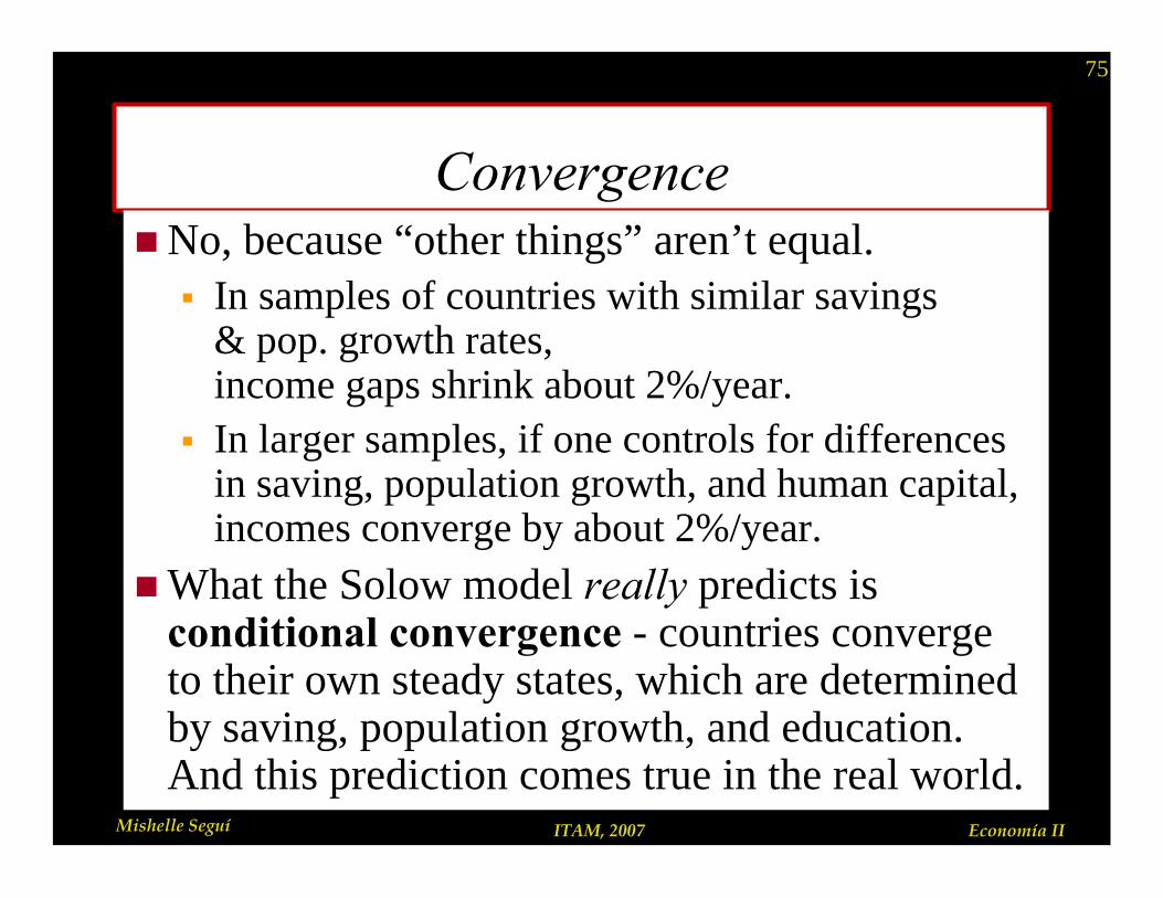
Convergence
n Solow model predicts that, other things equal, “poor” countries (with lower Y/L and K/L ) should grow faster than “rich” ones.
n If true, then the income gap between rich & poor countries would shrink over time, and living standards “converge.”
n In real world, many poor countries do NOT grow faster than rich ones. Does this mean the Solow model fails?
75
Mishelle Seguí ITAM, 2007 Economía II
ConvergencenNo, because “other things” aren’t equal. § In samples of countries with similar savings
& pop. growth rates, income gaps shrink about 2%/year.
§ In larger samples, if one controls for differences in saving, population growth, and human capital, incomes converge by about 2%/year.
nWhat the Solow model really predicts is conditional convergence - countries converge to their own steady states, which are determined by saving, population growth, and education. And this prediction comes true in the real world.

76
Mishelle Seguí ITAM, 2007 Economía II
Chapter summary
1. Key results from Solow model with tech progress§ steady state growth rate of income per person
depends solely on the exogenous rate of tech progress§ the U.S. has much less capital than the Golden
Rule steady state
2. Ways to increase the saving rate§ increase public saving (reduce budget deficit)§ tax incentives for private saving
77
Mishelle Seguí ITAM, 2007 Economía II
Chapter summary3. Productivity slowdown & “new economy”§ Early 1970s: productivity growth fell in the
U.S. and other countries. § Mid 1990s: productivity growth increased,
probably because of advances in I.T.
4. Empirical studies§ Solow model explains balanced growth,
conditional convergence§ Cross-country variation in living standards
due to differences in cap. accumulation and in production efficiency