alberto fraile 1,*, roberto martínez 2 and daniel fernández 3

Article

Jacob’s Ladder: Prime numbers in 2d

Alberto Fraile 1,*, Roberto Martínez 2 and Daniel Fernández 3

1 Czech Technical University Prague. Department of Control Engineering, Advanced Materials Group Praha 2,Karlovo námestí 13, E-s136, Czech Republic; [email protected]

2 Universidad del País Vasco - Euskal Herriko Unibertsitatea, Barrio Sarriena s/n 48940 Leioa. Bizkaia, Spain;[email protected]

3 University of Iceland, Science Institute, Dunhaga 3, 107 Reykjavík, Iceland; [email protected]* Correspondence: [email protected]

Version February 4, 2020 submitted to Math. Comput. Appl.

Abstract: Prime numbers are one of the most intriguing figures in mathematics. Despite centuries ofresearch, many questions remain still unsolved. In recent years, computer simulations are playing afundamental role in the study of an immense variety of problems. In this work, we present a simplerepresentation of prime numbers in two dimensions that allows us to formulate a number of conjecturesthat may lead to important avenues in the field of research on prime numbers. In particular, although thezeroes in our representation grow in a somewhat erratic, hardly predictable way, the gaps between thempresent a remarkable and intriguing property: a clear exponential decay in the frequency of gaps vs gapsize. The smaller the gaps, the more frequently they appear. Additionally, the sequence of zeroes, despitebeing non-consecutive numbers, contains a number of primes approximately equal to n/ log n , being nthe number of terms in the sequence.

Keywords: Prime numbers, Number theory, Number sequences

1. Introduction

Prime numbers have fascinated mathematicians since the beginnings of Mathematics (Ingham,Littlewood, Anglin, Apostol). Their distribution is intriguing and mysterious to some extent, despitebeing non-chaotic. After centuries of research there are still many open problems to be solved, andthe exact details of the prime numbers distribution are yet to be understood (Hardy (1979), Shanks).Today, the interest in prime numbers has received a new impulse after their unexpected appearancein different contexts ranging from cryptology (Stallings) or quantum chaos (Goles, Toha) to biology(Berry, Sakhr). Furthermore, with the advent of more and more powerful computers, different studiesare being undertaken where methods traditionally used by physicists are being applied to the studyof primes. For example, in (Wolf (1989)) the multifractality of primes was investigated, whereas someappropriately defined Lyapunov exponents for the distribution of primes were calculated numericallyin (Gamba). Additionally, one of the most studied problems in number theory, the Goldbach conjecture,first formulated around 1740, has been being continuously studied with the help of computers (Saouter,Richstein, Granville)1. More examples can be found in (Borwein).

1 Its weaker version, called the ternary Goldbach conjecture, was finally proven to be true in 2013 (Helfgott).

Submitted to Math. Comput. Appl., pages 1 – 17 www.mdpi.com/journal/mca

arX

iv:1

801.

0154

0v3

[m

ath.

HO

] 2

Feb

202

0

http://www.mdpi.com

http://www.mdpi.com/journal/mca

Version February 4, 2020 submitted to Math. Comput. Appl. 2 of 17

2. Jacob’s Ladder

One can argue that prime numbers present perplexing features, somewhat of a hybrid of localunpredictability and global regular behavior. It is this interplay between randomness and regularity whatmotivated searches for local and global patterns that could perhaps be signatures of more fundamentalmathematical properties.

Our work is concerned with the long standing question of the prime numbers distribution, or moreprecisely with the gaps between primes (Cramer, Erdos), a topic that has attracted much attention recently(Granville, Maynard (2016)) after some massive advances (Zhang). Some problems related to prime gapsare well known, for instance, Legendre’s conjecture states that there is a prime number between n2 and(n + 1)2 for every positive integer n. This conjecture is one of Landau’s problems on prime numbers (Guy)and up to date (2018) it is still waiting to be proved or disproved. Another example would be the famoustwin primes conjecture (Hardy (1923)). Proving this conjecture seemed to be far out of reach until justrecently. In 2013, Yitang Zhang demonstrated the existence of a finite bound B = 70, 000, 000, such thatthere are infinitely many pairs of distinct primes which differ by no more than B (Zhang). After such animportant breakthrough, proving the twin prime conjecture looked much more plausible. Immediatelyafter, a cooperative team led by Terence Tao, building upon Zhang’s techniques, was able to lower thatbound down to 4,680. Then in the same year, Maynard slashed the value of B down to 600, and finally thePolymath project further reduced it to 246 (Polymath, Maynard (2015)).

Displaying numbers in two dimensions has been a traditional approach toward primes visualization(Stein, Orlowski). Here we propose an original way of number arrangement yielding an appealing visualstructure: an oscillating plot that increases and decreases according to the prime number distribution. Weplot the integers from 1 to n in 2D (x, y) starting with 1 and y = 0 (hence, the first point will be (1, 0)),moving to 2 the plot moves up in the y axis, so that the next point in terms of coordinates is (2, 1). In thenext step, it goes up or down depending on whether the number n is a prime number or not. Number 2 isprime, so it flips in such a way that it goes down next, and hence the third point is (3, 0). Now, 3 is primeso the next step goes up again, and we move up to (4, 1). Number 4 is not a prime so it continues movingup, and so on. We used our own code but different codes to produce Jacob’s ladder can be found in theOn-Line Encyclopedia of Integer Sequences (OEIS).

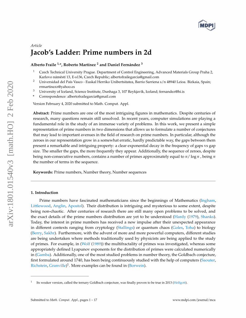
In Fig. 1 the sequence produced by the algorithm is shown up to n = 50. The blue dashed line standsfor the y = 0 line (or x axis), which will be central to our study. We will refer to the points (x, 0) as zeroesfrom now on. Because of the resemblance of this numerical structure to a ladder, we refer to this set ofpoints in the 2D plane as Jacob’s Ladder, J(n) for short hereafter. The points in the ladder (the y values) canbe written as:

J(n) =n

∑k=1

(−1)π(k) (2.1)

where π(n) denotes the number of primes ≤ n.

3. Results

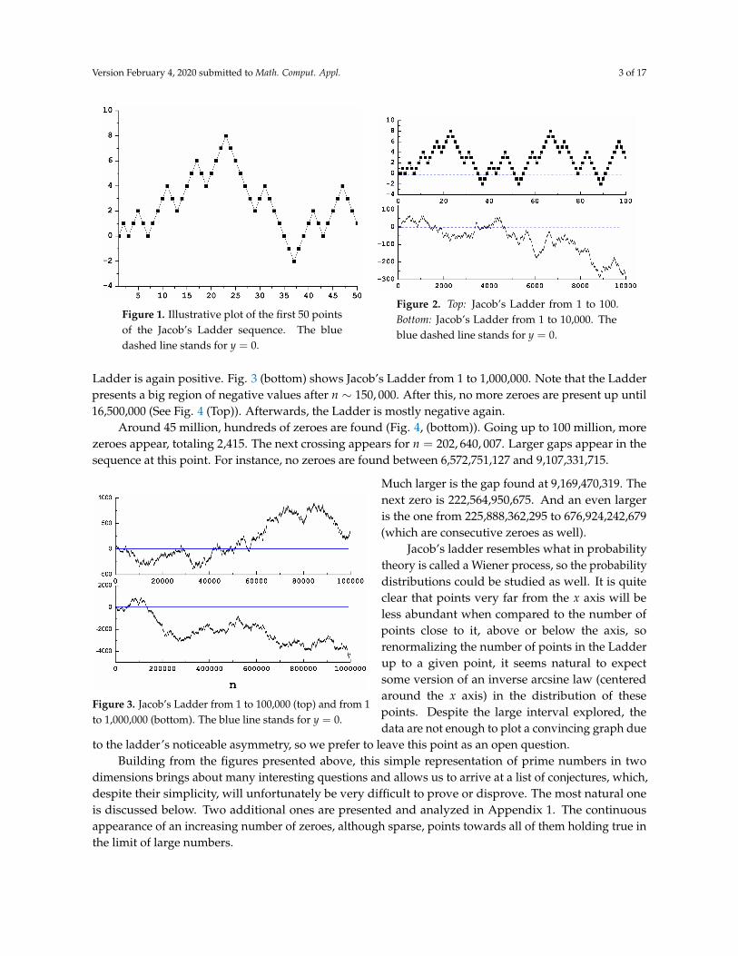
The next figures show the numerical results which inspired the ideas and conjectures we will presentin the next section. Fig. 2 (Top) shows Jacob’s Ladder from 1 to 100. The blue dashed line signals the x axisfor clarity shake. As can be seen, up to 100 the Ladder is almost positive, being most of its points abovethe x axis. This is misleading, though, as we can see from looking at the behavior of Jacob’s Ladder from 1to 10,000 (Fig. 2 (Bottom)).

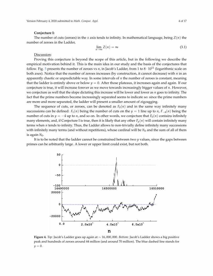
Fig. 2 (bottom) shows Jacob’s Ladder from 1 to 10,000. As can be seen, now most of the Ladder isnegative except for two regions. However, this fact changes again if we move to higher values. Fig. 3 (top)shows Jacob’s Ladder from 1 to 100,000 and here we see, as said before, that after n ∼ 50, 000 most of the


Figure 1. Illustrative plot of the first 50 pointsof the Jacob’s Ladder sequence. The bluedashed line stands for y = 0.

Figure 2. Top: Jacob’s Ladder from 1 to 100.Bottom: Jacob’s Ladder from 1 to 10,000. Theblue dashed line stands for y = 0.

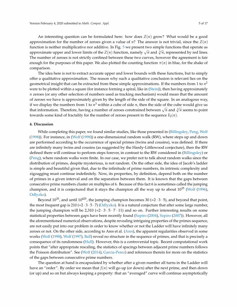
Ladder is again positive. Fig. 3 (bottom) shows Jacob’s Ladder from 1 to 1,000,000. Note that the Ladderpresents a big region of negative values after n ∼ 150, 000. After this, no more zeroes are present up until16,500,000 (See Fig. 4 (Top)). Afterwards, the Ladder is mostly negative again.

Around 45 million, hundreds of zeroes are found (Fig. 4, (bottom)). Going up to 100 million, morezeroes appear, totaling 2,415. The next crossing appears for n = 202, 640, 007. Larger gaps appear in thesequence at this point. For instance, no zeroes are found between 6,572,751,127 and 9,107,331,715.

Figure 3. Jacob’s Ladder from 1 to 100,000 (top) and from 1to 1,000,000 (bottom). The blue line stands for y = 0.

Much larger is the gap found at 9,169,470,319. Thenext zero is 222,564,950,675. And an even largeris the one from 225,888,362,295 to 676,924,242,679(which are consecutive zeroes as well).

Jacob’s ladder resembles what in probabilitytheory is called a Wiener process, so the probabilitydistributions could be studied as well. It is quiteclear that points very far from the x axis will beless abundant when compared to the number ofpoints close to it, above or below the axis, sorenormalizing the number of points in the Ladderup to a given point, it seems natural to expectsome version of an inverse arcsine law (centeredaround the x axis) in the distribution of thesepoints. Despite the large interval explored, thedata are not enough to plot a convincing graph due

to the ladder’s noticeable asymmetry, so we prefer to leave this point as an open question.Building from the figures presented above, this simple representation of prime numbers in two

dimensions brings about many interesting questions and allows us to arrive at a list of conjectures, which,despite their simplicity, will unfortunately be very difficult to prove or disprove. The most natural oneis discussed below. Two additional ones are presented and analyzed in Appendix 1. The continuousappearance of an increasing number of zeroes, although sparse, points towards all of them holding true inthe limit of large numbers.


Conjecture I:The number of cuts (zeroes) in the x axis tends to infinity. In mathematical language, being Z(n) the

number of zeroes in the Ladder,lim

n→∞Z(n) = ∞ (3.1)

Discussion:Proving this conjecture is beyond the scope of this article, but in the following we describe the

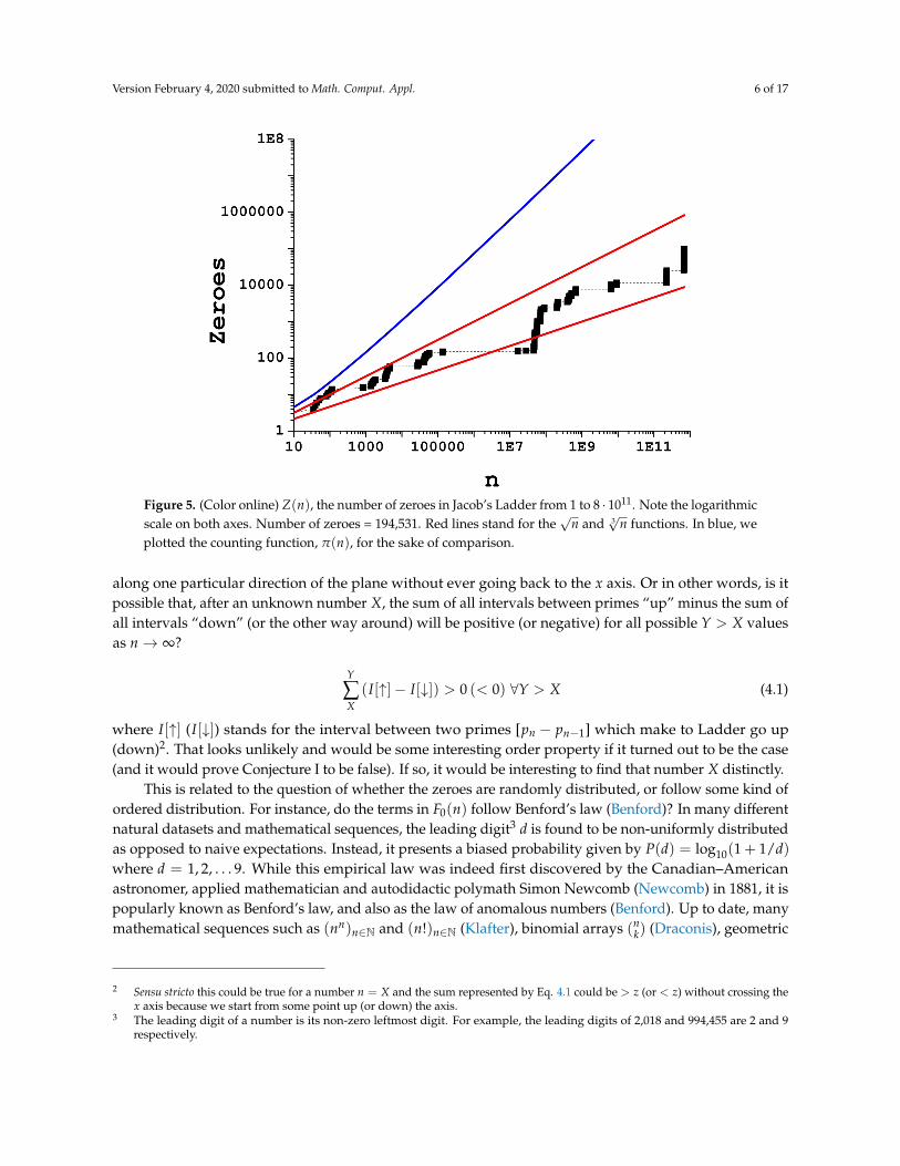
empirical motivation behind it. This is the main idea in our study and the basis of the conjectures thatfollow. Fig. 5 presents the number of zeroes vs n, in Jacob’s Ladder, from 1 to 8 · 1011 (logarithmic scale onboth axes). Notice that the number of zeroes increases (by construction, it cannot decrease) with n in anapparently chaotic or unpredictable way. In some intervals of n the number of zeroes is constant, meaningthat the ladder is entirely above or below y = 0. After those plateaus, it increases again and again. If ourconjecture is true, it will increase forever as we move towards increasingly bigger values of n. However,we conjecture as well that the slope dictating this increase will be lower and lower as n goes to infinity. Thefact that the prime numbers become increasingly separated seems to indicate so: since the prime numbersare more and more separated, the ladder will present a smaller amount of zigzagging.

The sequence of cuts, or zeroes, can be denoted as F0(n) and in the same way infinitely manysuccessions can be defined: F1(n) being the number of cuts on the y = 1 line up to n, F−4(n) being thenumber of cuts in y = −4 up to n, and so on. In other words, we conjecture that F0(n) contains infinitelymany elements, and, if Conjecture I is true, then it is likely that any other Fy(n) will contain infinitely manyterms when n tends to infinity. Thus, the Ladder allows to non-trivially define infinitely many successionswith infinitely many terms (and without repetitions), whose cardinal will be ℵ0 and the sum of all of themis again ℵ0.

It is to be noted that the ladder cannot be constrained between two y values, since the gaps betweenprimes can be arbitrarily large. A lower or upper limit could exist, but not both.

Figure 4. Top: Jacob’s Ladder goes up again at ∼ 16, 000, 000. Bottom: Jacob’s Ladder shows a big positivepeak and hundreds of zeroes around 44 million (and around 70 million). The blue dashed line stands fory = 0.


An interesting question can be formulated here: how does Z(n) grow? What would be a goodapproximation for the number of zeroes given a value of n? The answer is not trivial, since the Z(n)function is neither multiplicative nor additive. In Fig. 5 we present two simple functions that operate asapproximate upper and lower limits of the Z(n) function, namely

√n and 3

√n, represented by red lines.

The number of zeroes is not strictly confined between these two curves, however the agreement is fairenough for the purposes of this paper. We also plotted the counting function π(n) in blue, for the shake ofcomparison.

The idea here is not to extract accurate upper and lower bounds with these functions, but to simplyoffer a qualitative approximation. The reason why such a qualitative conclusion is relevant lies on thegeometrical insight that can be extracted from these simple approximations. If the numbers from 1 to n2

were to be plotted within a square (for instance forming a spiral, like in (Stein)), then having approximatelyn zeroes (or any other selection of numbers used as tracking mechanism) would mean that the amountof zeroes we have is approximately given by the length of the side of the square. In an analogous way,if we display the numbers from 1 to n3 within a cube of side n, then the side of the cube would give usthat information. Therefore, having a number of zeroes constrained between

√n and 3

√n seems to point

towards some kind of fractality for the number of zeroes present in the sequence F0(n).

4. Discussion

While completing this paper, we found similar studies, like those presented in (Billingsley, Peng, Wolf(1998)). For instance, in (Wolf (1998)) a one-dimensional random walk (RW), where steps up and downare performed according to the occurrence of special primes (twins and cousins), was defined. If thereare infinitely many twins and cousins (as suggested by the Hardy-Littlewood conjecture), then the RWdefined there will continue to perform steps forever, in contrast to the RW considered in (Billingsley) or(Peng), where random walks were finite. In our case, we prefer not to talk about random walks since thedistribution of primes, despite mysterious, is not random. On the other side, the idea of Jacob’s ladderis simple and beautiful given that, due to the infinitude of prime numbers, its intrinsic complexity andzigzagging must continue indefinitely. Now, its properties, by definition, depend both on the numberof primes in a given interval and on the separation between them. It is known that the gaps betweenconsecutive prime numbers cluster on multiples of 6. Because of this fact 6 is sometimes called the jumpingchampion, and it is conjectured that it stays the champion all the way up to about 1035 (Wolf (1996),Odlyzko).

Beyond 1035, and until 10425, the jumping champion becomes 30 (=2 · 3 · 5), and beyond that point,the most frequent gap is 210 (=2 · 3 · 5 · 7) (Odlyzko). It is a natural conjecture that after some large number,the jumping champion will be 2,310 (=2 · 3 · 5 · 7 · 11) and so on. Further interesting results on somestatistical properties between gaps have been recently found (Szpiro (2004), Szpiro (2007)). However, allthe aforementioned numerical observations, despite revealing intriguing properties of the primes sequence,are not easily put into our problem in order to know whether or not the Ladder will have infinitely manyzeroes or not. On the other side, according to Ares et al. (Ares), the apparent regularities observed in someworks (Wolf (1998), Wolf (1997), Ball) reveal no structure in the sequence of primes, and that is precisely aconsequence of its randomness (Hull). However, this is a controversial topic. Recent computational workpoints that “after appropriate rescaling, the statistics of spacings between adjacent prime numbers followsthe Poisson distribution”. See (Wolf (2014), Garcia-Perez) and references therein for more on the statisticsof the gaps between consecutive prime numbers.

The question at hand is encapsulated by whether after a given number all turns in the Ladder willhave an “order”. By order we mean that J(n) will go up (or down) after the next prime, and then down(or up) and so on but always keeping a property: that an “averaged” curve will continue asymptotically


Figure 5. (Color online) Z(n), the number of zeroes in Jacob’s Ladder from 1 to 8 · 1011. Note the logarithmicscale on both axes. Number of zeroes = 194,531. Red lines stand for the

√n and 3

√n functions. In blue, we

plotted the counting function, π(n), for the sake of comparison.

along one particular direction of the plane without ever going back to the x axis. Or in other words, is itpossible that, after an unknown number X, the sum of all intervals between primes “up” minus the sum ofall intervals “down” (or the other way around) will be positive (or negative) for all possible Y > X valuesas n→ ∞?

Y

∑X(I[↑]− I[↓]) > 0 (< 0) ∀Y > X (4.1)

where I[↑] (I[↓]) stands for the interval between two primes [pn − pn−1] which make to Ladder go up(down)2. That looks unlikely and would be some interesting order property if it turned out to be the case(and it would prove Conjecture I to be false). If so, it would be interesting to find that number X distinctly.

This is related to the question of whether the zeroes are randomly distributed, or follow some kind ofordered distribution. For instance, do the terms in F0(n) follow Benford’s law (Benford)? In many differentnatural datasets and mathematical sequences, the leading digit3 d is found to be non-uniformly distributedas opposed to naive expectations. Instead, it presents a biased probability given by P(d) = log10(1 + 1/d)where d = 1, 2, . . . 9. While this empirical law was indeed first discovered by the Canadian–Americanastronomer, applied mathematician and autodidactic polymath Simon Newcomb (Newcomb) in 1881, it ispopularly known as Benford’s law, and also as the law of anomalous numbers (Benford). Up to date, manymathematical sequences such as (nn)n∈N and (n!)n∈N (Klafter), binomial arrays (n

k) (Draconis), geometric

2 Sensu stricto this could be true for a number n = X and the sum represented by Eq. 4.1 could be > z (or < z) without crossing thex axis because we start from some point up (or down) the axis.

3 The leading digit of a number is its non-zero leftmost digit. For example, the leading digits of 2,018 and 994,455 are 2 and 9respectively.


Figure 6. (Color online) Leading digit histogram of the zeroes sequence F0(n). The proportion of thedifferent leading digits found in the intervals, [1, 1010], [1, 1011] and in [1, 8 · 1011] is shown in black squares,red diamonds and green circles as labeled. The expected values according to Benford’s law are shown inblue triangles.

Figure 7. (Color online) Number of primes as a function of the number of terms (zeroes) in the sequenceF0(n). The red line stands for the plausible similitude with the counting function π(n) ∼ n/ log n.

sequences or sequences generated by recurrence relations (Raimi, Takloo-Bighash), to cite a few, have beenproved to conform to Benford.


Fig. 6 shows the proportion of the different leading digits found in the different intervals [1, n], upto 194,531 zeroes, and the expected values according to Benford’s law. Note that intervals [1, n] havebeen chosen such that n = 10D, with D a natural integer, in order to ensure an unbiased sample whereall possible first digits are a priori equiprobable. With that in mind, however, the results for the interval[1, 8 · 1011] are also presented because the number of zeroes are many times more than those found up to1011. Obviously, the curve is likely to change as more and more zeroes are counted (it changes when fewerzeroes are counted). A straightforward calculation demonstrates that, in the best of cases, one shouldcount up to five (or six) times the current number of zeroes before having a distribution in fair agreementwith Benford’s law. Note that in order to obtain such large amount of zeroes, according to Fig. 5, it is likelythat one should explore the Ladder in a 25 (36) or 125 (216) times larger interval, i.e. up to 1014 (1.7 · 1014).

On the other hand, it is natural to assume that the distribution presented by F0(n) will be the samefor all values of y. Thus, while being aware that the numbers are still very small from a statistical point ofview, the analysis of the terms in more crowded sequences can provide further evidence for the randomdistribution (or better said, non-Benford-like distribution) of Fy(n) for all y.

Another point to be noticed is that all of the zeroes can be written as (4n + 3). This is not a surprise,in fact it can be easily proved that it must be this way: after 3, which is the first zero excluding 1, all zeroesmust be separated by a number twice the sum of the number of gaps between primes (every pair of primesis separated by an even number), therefore the gaps between zeroes will be always a multiple of 4.

For one more test about some possible unexpected non-random properties of the zeroes in the Ladderwe can check the number of zeroes ending in a given odd digit (since all the even ones will not be in F0(n)).Doing so we observe they change depending on the explored interval, so there is no clear evidence of anytrend 4.

But going back to the zeroes as a whole, we can observe the two most important results foundin our study. First, it is natural to wonder: how many of these zeroes are primes? Is this numbersomewhere predictable? Since in an interval [1, n] we find ∼ n/ log n primes, should we expect, in a setof X consecutive zeroes (but not consecutive numbers!), an amount of primes approximately equal toX/ log X? Interestingly, it seems to be the case if we count a few thousands of zeroes when looking at Fig.7, but it is not really the case from looking at the differences in percentage (see Table 1). The prime zeroesfound are nevertheless in remarkable agreement with this simple assumption. As we see in Fig. 7, forn > 109 the prime numbers found in F0(n) depart steadily from n/ log n, being the latter an overestimateof the actual number of primes.

As mentioned before, all zeroes can be written as (4n + 3). But 4n + 3 is the same as 4(n + 1)− 1.It is a well known result that all primes (except 2) can be written as 4n + 1 or 4n − 1 - the first onesallowing to be expressed as the sum of two perfect squares p = x2 + y2, while the second ones can neverbe expressed in such a way. Therefore in our results, those zeroes which are prime always belong to thesecond subgroup. Furthermore, the arithmetic progressions 4n± 1, (and 6n± 1) are of particular interestbecause the primes in the progression 4n− 1 (and 6n− 1) are known to be "denser" than in the progression4n + 1 (and 6n + 1); a result conjectured in 1853 by Tschebyschef (Dickson, Tschebyschef) and proved byPhragmen (Phragmen) and Landau (Landau). However, the problem is, as is usually the case in numbertheory, far from being simple. A famous result by Littlewood (Littlewood) showed that there are infinitely

4 The terms ending in 1, 3, 5, 7 and 9 amount to 38,835, 38,905, 38,799, 38,898 and 39,093 respectively in the first 194,530 zeroes,thus showing a uniform distribution (∼ 20% each). A linear fit (y = a + bx) to the data (in probabilities, given as %) provides thefollowing result: a = 19.93459 (0.04315) and b = 0.01308 (0.00751). The slope is small, and just twice the error of the linear fit, soit is quite unsafe to assume a trend on this.


many integers x such that there are more prime numbers in the progression 4n + 1 than in the 4n− 1, upto that number x 5.

It is easy to see that every sequence Fb(x) (or zeroes in the lines y = b) will contain primes (thatis, reversals of the ladder) if and only if b is even. In particular if b = 4a, with a an integer number orzero, then those primes will belong to the arithmetic progression 4n− 1. Besides, those sequences whereb = 4a ± 2 will contain primes belonging to the arithmetic progression 4n + 1 (with the exception of2, there are no primes in the Fb(x) sequences when b is odd). Thus, it is clear that the problem of howto demonstrate the existence of an infinite number of zeroes in Jacob’s Ladder is related with previousimportant results regarding primes in arithmetic progressions. However, it is not enough to know howmany primes are found in a particular progression: the gaps between primes are equally important, andthat is a more mysterious problem.

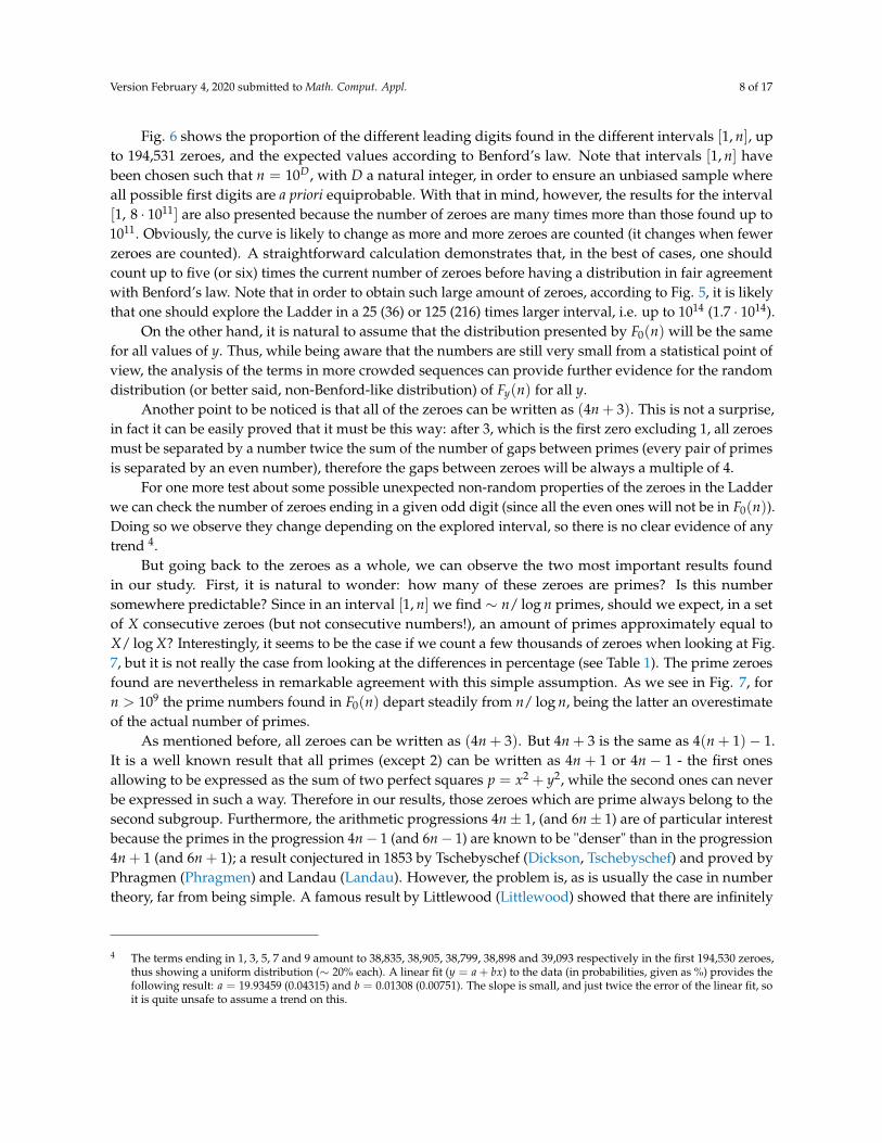
Now we will see what can be said about gaps: how are the zeroes separated? As we have seen in theFigures 1 to 4, the Ladder goes up and down in an erratic way, resulting in a rather capricious distributionof the zeroes. Nevertheless, counting the number of times that a given gap between zeroes appears withina given number of zeroes, the result is clearly non-arbitrary. Fig. 8 shows the result after analyzing thegaps in F0(n) up to 8 · 1011. It can be seen that a clear exponential decay is found. Note as well that allgaps are multiples of 4, except 2, which only appears once (The demonstration of the fact that all gaps aremultiples of 4 is trivial).

The inset shows the averaged gap, Γ, vs the interval size. Γ is calculated as the sum of gaps dividedby the number of gaps. Another possible definition, Ξ, would be the interval size divided by the numberof zeroes. The plateaus are due to intervals (from 106 to 107 for instance) where no more zeroes are found,so the number of gaps is constant. Using the Ξ definition, the averaged gap would be 10 times larger.

Fig. 8, showing the distribution of gaps, is a remarkable result and it may lead to a number ofinteresting observations. Note that almost 25% of the gaps are 4, 8, 12, or 16, and more than 53% of thegaps are smaller than 60. Gaps 6 100 represent more than 63% of the gaps found, however, as said before,very large gaps are found as well as large as 451,035,880,384 (about half the interval explored).

In the intervals explored up to now, 4 is always the most frequent gap, referred to as γ1 hereafter,followed by γ2= 8, γ3= 12 (i.e. the second most frequent gap is 8, the third most frequent is 12, etc.).Immediately, a legitimate and important question would be to inquire about the behavior of the distributionof gaps for large values of n. Will γ1 be 4 for any interval, no matter how large? Or is it possible thatfrom a very large interval onwards, it shifts to 8, and later on to 12, and so on? Furthermore, it could bereasonable as well to expect an equiprobable distribution of gaps in the limit n→ ∞.

However, it has been shown that 4 is the most probable gap size (Fig. 8). If the exponential decay ofγn vs n hypothesis were finally confirmed ∀n, such result would represent an attribute of the Ladder offundamental importance, meaning that every time that the ladder crosses the x axis, it is close to a primenumber. This observation can be misleading, though, because at the same time the average gap clearlyseems to increase with n (Inset in Fig. 8). So these results do not mean that all of the zeroes are primes. Infact, as showed before (See Fig. 7 and Table 1), out of n zeroes, about n/ log n are actually primes.

The percentage of gaps of length 4 decreases with n faster than exponentially, in the same way asthose of length 8 or 12, and likely for all gap values (in small intervals some variations may occur, but weare interested in properties appearing in the limit of large intervals), as shown in Fig. 9. This result can beeasily explained since the larger the interval is, the more gaps enter in the list of gaps, so it is natural thatthe percentage would decrease.

5 Using formal mathematical notation, it is said that π4,3(x) < π4,1(x) for infinitely many x, where πb,c(x) denotes the number ofpositive primes ≤ x which are equal to c (mod b).


Figure 8. Number of times that a gap appears depending on the the gap size, only up to 1000 for clarityshake. The red line presents the exponential decay fit. The inset shows the averaged gap Γ vs the intervalsize.

At the same time, since the average gap increases, it could be natural to expect an increase in thepercentage of larger gaps. But that is not the case – only for small intervals do we observe an increasewith n of the percentage of large gaps, because for small intervals large gaps are rare, yet it seems that thepercentage of large gaps is always below that of 4, 8 etc.

A final important remark: we started this work without knowing any previous studies on this topic.Only while writing down the paper that we checked if the sequence of zeroes appeared in the On-LineEncyclopedia of Integer Sequences (OEIS), and then we found it was first studied in 2001 by Jason Earlsand subsequently by Hans Havermann within a different context 6 and Don Reble 7.

5. Conclusions

In this paper, an original idea has been proposed with the aim of arranging integers in 2D accordingto the occurrence of primality. This arrangement of numbers resembles a ‘ladder’ and displays peaksand valleys at the positions of the primes. Numerical studies have been undertaken in order to extractqualitative information from such a representation. As a result of those studies, it is possible to promotefour observations in the category of conjectures. One may easily state that the ladder, from its ownconstruction, will cross the horizontal axis an indefinite number of times; namely, the ladder will haveinfinitely many zeroes.

The number of zeroes grows in a hardly predictable way, somewhere between√

n and 3√

n, but thenumber of primes in F0(n) is very well fitted by n/ log n for small numbers (up to 10,000 zeroes). However,

6 See full sequence in http://chesswanks.com/num/a064940.txt.7 See full sequence in https://oeis.org/A064940/a064940.txt.

http://chesswanks.com/num/a064940.txt

https://oeis.org/A064940/a064940.txt


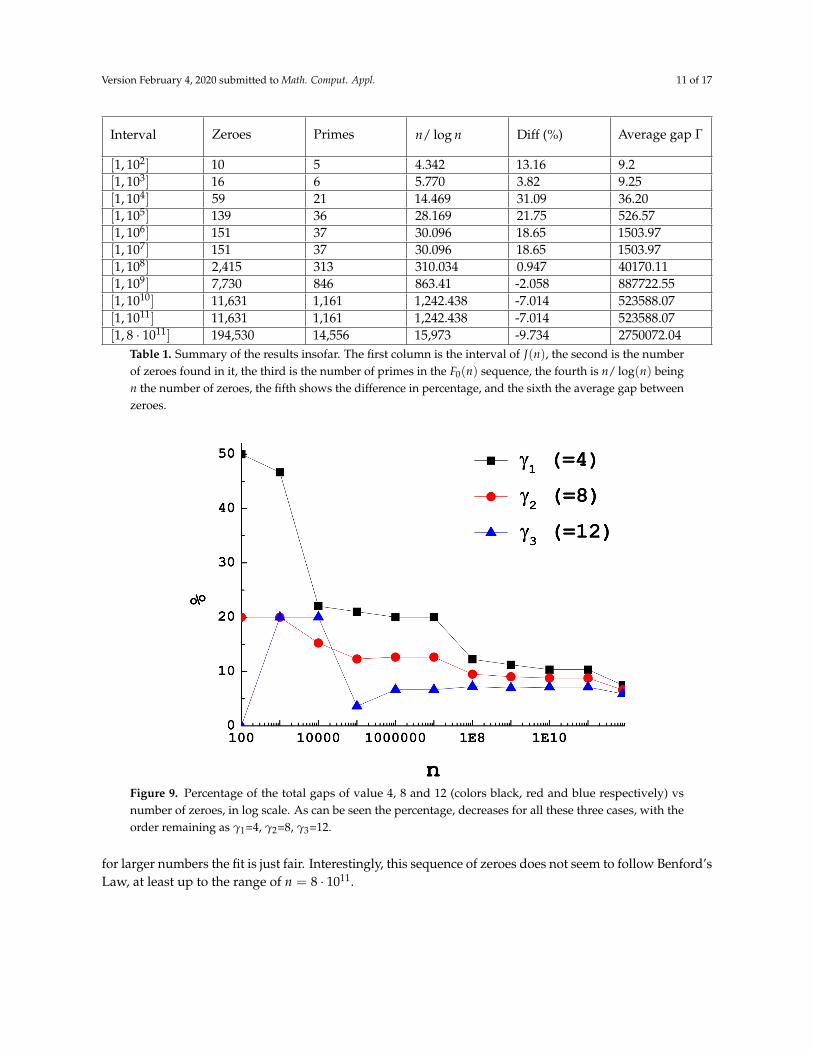
Interval Zeroes Primes n/ log n Diff (%) Average gap Γ

[1, 102] 10 5 4.342 13.16 9.2[1, 103] 16 6 5.770 3.82 9.25[1, 104] 59 21 14.469 31.09 36.20[1, 105] 139 36 28.169 21.75 526.57[1, 106] 151 37 30.096 18.65 1503.97[1, 107] 151 37 30.096 18.65 1503.97[1, 108] 2,415 313 310.034 0.947 40170.11[1, 109] 7,730 846 863.41 -2.058 887722.55[1, 1010] 11,631 1,161 1,242.438 -7.014 523588.07[1, 1011] 11,631 1,161 1,242.438 -7.014 523588.07[1, 8 · 1011] 194,530 14,556 15,973 -9.734 2750072.04

Table 1. Summary of the results insofar. The first column is the interval of J(n), the second is the numberof zeroes found in it, the third is the number of primes in the F0(n) sequence, the fourth is n/ log(n) beingn the number of zeroes, the fifth shows the difference in percentage, and the sixth the average gap betweenzeroes.

Figure 9. Percentage of the total gaps of value 4, 8 and 12 (colors black, red and blue respectively) vsnumber of zeroes, in log scale. As can be seen the percentage, decreases for all these three cases, with theorder remaining as γ1=4, γ2=8, γ3=12.

for larger numbers the fit is just fair. Interestingly, this sequence of zeroes does not seem to follow Benford’sLaw, at least up to the range of n = 8 · 1011.


Furthermore, no trend is apparent looking at the last digit of the zeroes, being all digits (1, 3, 5, 7 and9 only) equiprobable. Thus, we have shown that the distribution of zeroes is, if not "random"8, at leastrather capricious. On the other hand, the gaps between zeroes present a remarkably well defined trend,displaying an exponential decay according to the size, the length of the gap and the frequency with whichit appears. This important result echoes previous studies regarding gaps between primes, such as thosepresented in (Wolf (1998), Szpiro (2004), Szpiro (2007), Ares, Wolf (1997), Ball, Wolf (2014), Garcia-Perez).Whether or not this will be true for any given interval is another open question.

Our theoretical predictions are largely based on intuition, but we provide qualitative support fromour preliminary results. Although the behaviors reported here have been validated only for n as large as8 · 1011, it is reasonable to expect that they would be observed for any arbitrary n. However, mathematicalproofs for our conjectures are likely to be extremely difficult since they are inextricably intertwined withthe still mysterious distribution of prime numbers.

To conclude, the algorithm9 of Jacob’s Ladder exhibits a remarkable feature despite its simplicity: Mostof the zeroes are close to prime numbers since the smaller the gaps are, the more frequently they appear.This important result represents an unexpected correlation between the apparently chaotic sequence, thezeroes in J(n), and the prime numbers distribution.

Appendix A. Additional conjectures

Conjecture II:The slope ε(n), of the Ladder is zero in the limit when n goes to infinity.

Discussion:The Ladder could have a finite (although we conjecture this not to be case) amount of zeroes, so that

after a certain number X, all points would be either above or below the x axis, and hence the slope wouldbe positive or negative in consequence. Note that even if Conjecture I is false, the slope could decreasecontinuously when n increases. And obviously if Conjecture I is true, then Conjecture II is more likely, butstill not necessarily true.

It is important to note that an arbitrarily large amount of zeroes does not imply ε = 0. This canbe proved with a simple counterexample, as shown in Fig. A1 (upper panel), where a simple ladder isconstructed by stacking triangles, each one three times higher than the previous one. This ladder will havean infinite number of zeroes by construction, but as can be easily seen, the slope ε is not zero (The lowerpanel in Fig. A1 shows the values of ε vs the number of points).

A clearer picture of the late behavior of Jacob’s ladder can be ascertained from an analysis of the gapsand the frequency with which they appear, as we discuss in Sec. 4. Under closer inspection, a pattern withsigns of predictability arises, allowing us to get an intuition on how the ladder is likely to extend towardsinfinity, much in the same way that a physicist would extrapolate statistically. To which extent one shouldtrust that intuition is not a matter of debate for the present paper.

8 How random are the zeroes in the sequence? Naively one would assume them to be as random as the prime number distribution.It is beyond the scope of this work to answer this question, but it would be worthy to study the randomness of this sequence (orany other Fy(n) created with this scheme) by using advanced randomness tests (Cacert, Marsaglia, Tsang).

9 The program is available under request.


For these reasons, we argue that Conjecture II is true even if Conjecture I is not. Now a different,more complex question is how fast ε(n)→ 0. The value of ε(n) is obtained by fitting the Ladder to y = b xfollowing a least squares approach

b =n ∑ xiyi −∑ xi ∑ yi

n ∑ x2i − (∑ xi)

2 . (A1)

Whether the slope b tends to zero or not depends on the difference between the terms of the numerator,which is where the prime numbers define the Ladder through the yi, which are unknown a priori (the xivalues are known for all i). Many important papers have been published in the last decades - see (Wolf(1989), Gamba, Cramer, Erdos, Maynard (2016), Zhang, Guy, Hardy (1923), Polymath, Maynard (2015),Stein, Wolf (1998), Wolf (1996), Odlyzko, Szpiro (2004), Szpiro (2007), Ares, Wolf (1997), Ball, Wolf (2014),Garcia-Perez) to name a few - some of which could help or show the way to calculate certain upper (and/orlower) limits for ε(n) in the limit when n tends to infinity. It seems to be a problem that could be attackedusing methods of probabilistic number theory (Kubilius, Kowalski), however, it is beyond the scope of thispaper to prove this conjecture.

A first naive idea could be to assume that the slope is of the same order of magnitude as n/π(n)n , that

is to say, 1/π(n), where π(n) is the prime-counting function as usual (See Fig. A2). It is to be mentionedthat Fig. A2 plots the absolute value of b , but this value can be positive or negative. It goes withoutsaying that the slope will depend not only on the number of primes, but also on their order, which isunknown a priori.10. The 1/π(n) model seems however to be an underestimate of ε(n), suggesting that

10 The slope is plotted up to 108 due to computational limitations. A way of calculating the slope of billions of points would be to"sift" or "filter" them, that is to say, to take only 1 every 100 or every 1000, etc. The error, however, is rather difficult to determine.

Figure A2. (Color online) Slope ε(n) of Jacob’s Ladder from 100 to 100,000,000 in logarithmic scale. Blackfull squares are the numerical values (obtained by fitting the Ladder to y = b x), while red empty circles,black empty squares and blue/green triangles are simple models. Orange squares are the values obtainedaveraging both green and blue points (see text).


√1/π(n) could be a better approximation. Obviously one can always obtain a better fit by adding one

more parameter to some function, in this case, a power to 1/π(n).

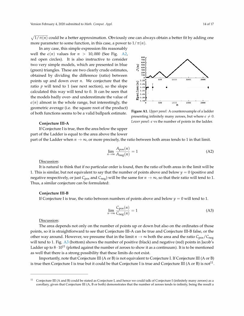
Figure A1. Upper panel: A counterexample of a ladderpresenting infinitely many zeroes, but where ε 6= 0.Lower panel: ε vs the number of points in the ladder.

In any case, this simple expression fits reasonablywell the ε(n) values for n > 10, 000 (See Fig. A2,red open circles). It is also instructive to considertwo very simple models, which are presented in blue(green) triangles. These are two clearly crude estimates,obtained by dividing the difference (ratio) betweenpoints up and down over n. We conjecture that theratio p will tend to 1 (see next section), so the slopecalculated this way will tend to 0. It can be seen thatthe models badly over- and underestimate the value ofε(n) almost in the whole range, but interestingly, thegeometric average (i.e. the square root of the product)of both functions seems to be a valid ballpark estimate.

Conjecture III-AIf Conjecture I is true, then the area below the upper

part of the Ladder is equal to the area above the lowerpart of the Ladder when n→ ∞, or more precisely, the ratio between both areas tends to 1 in that limit.

limn→∞

Apos(n)Aneg(n)

= 1 (A2)

Discussion:It is natural to think that if no particular order is found, then the ratio of both areas in the limit will be

1. This is similar, but not equivalent to say that the number of points above and below y = 0 (positive andnegative respectively, or just Cpos and Cneg) will be the same for n→ ∞, so that their ratio will tend to 1.Thus, a similar conjecture can be formulated:

Conjecture III-BIf Conjecture I is true, the ratio between numbers of points above and below y = 0 will tend to 1.

limn→∞

Cpos(n)Cneg(n)

= 1 (A3)

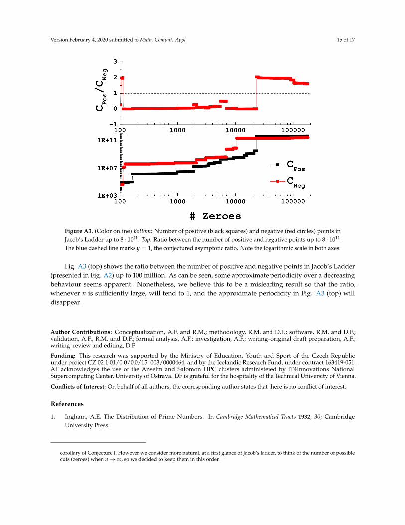
Discussion:The area depends not only on the number of points up or down but also on the ordinates of those

points, so it is straightforward to see that Conjecture III-A can be true and Conjecture III-B false, or theother way around. However, we presume that in the limit n→ ∞ both the area and the ratio Cpos/Cneg

will tend to 1. Fig. A3 (bottom) shows the number of positive (black) and negative (red) points in Jacob’sLadder up to 8 · 1011 (plotted against the number of zeroes to show it as a continuum). It is to be mentionedas well that there is a strong possibility that these limits do not exist.

Importantly, note that Conjecture III (A or B) is not equivalent to Conjecture I. If Conjecture III (A or B)is true then Conjecture I is true but it could be that Conjecture I is true and Conjecture III (A or B) is not11.

11 Conjecture III (A and B) could be stated as Conjecture I, and hence we could talk of Conjecture I (infinitely many zeroes) as acorollary, given that Conjecture III (A, B or both) demonstrates that the number of zeroes tends to infinity, being the result a


Figure A3. (Color online) Bottom: Number of positive (black squares) and negative (red circles) points inJacob’s Ladder up to 8 · 1011. Top: Ratio between the number of positive and negative points up to 8 · 1011.The blue dashed line marks y = 1, the conjectured asymptotic ratio. Note the logarithmic scale in both axes.

Fig. A3 (top) shows the ratio between the number of positive and negative points in Jacob’s Ladder(presented in Fig. A2) up to 100 million. As can be seen, some approximate periodicity over a decreasingbehaviour seems apparent. Nonetheless, we believe this to be a misleading result so that the ratio,whenever n is sufficiently large, will tend to 1, and the approximate periodicity in Fig. A3 (top) willdisappear.

Author Contributions: Conceptualization, A.F. and R.M.; methodology, R.M. and D.F.; software, R.M. and D.F.;validation, A.F., R.M. and D.F.; formal analysis, A.F.; investigation, A.F.; writing–original draft preparation, A.F.;writing–review and editing, D.F.

Funding: This research was supported by the Ministry of Education, Youth and Sport of the Czech Republicunder project CZ.02.1.01/0.0/0.0/15_003/0000464, and by the Icelandic Research Fund, under contract 163419-051.AF acknowledges the use of the Anselm and Salomon HPC clusters administered by IT4Innovations NationalSupercomputing Center, University of Ostrava. DF is grateful for the hospitality of the Technical University of Vienna.

Conflicts of Interest: On behalf of all authors, the corresponding author states that there is no conflict of interest.

References

1. Ingham, A.E. The Distribution of Prime Numbers. In Cambridge Mathematical Tracts 1932, 30; CambridgeUniversity Press.

corollary of Conjecture I. However we consider more natural, at a first glance of Jacob’s ladder, to think of the number of possiblecuts (zeroes) when n→ ∞, so we decided to keep them in this order.


2. Littlewood, J.E. Sur les distribution des nombres premiers. Comptes Rendus Acad. Sci. Paris bf 1914 158, 1869–1872;Littlewood, J.E. Sur la distribution des nombres premiers. Comptes Rendus 1914, v. 158, pp. 1869-1872.

3. Anglin, W.S. The Queen of Mathematics: An Introduction to Number Theory; Dordrecht, Netherlands: Kluwer, 1995.4. Apostol, T.M. Introduction to Analytic Number Theory; New York: Springer-Verlag, 1976.5. Hardy, G.H. and Wright, W.M. Unsolved Problems Concerning Primes. In An Introduction to the Theory of Numbers;

5th Ed.; Oxford University Press: Oxford, UK, 1979; pp. 19 and 415–416.6. Shanks, D. Solved and Unsolved Problems in Number Theory; New York: Chelsea, 1985; pp. 30-31 and 222.7. Stallings, M. Cryptography and Network Security: Principles and Practice; Prentice-Hall; New Jersey, 1999.8. Goles, E., Schulz, O. and Markus, M. Prime number selection of cycles in a predator-prey model. Complexity

2001, 6, 33–38.9. Toha, J. and Soto, M.A. Biochemical identification of prime numbers. Medical Hypothesis bf 1999, 53, 361.10. Berry, M.V. Quantum chaology, prime numbers and Riemann’s zeta function. Inst. Phys. Conf. Ser. 1993, 133,

133–134.11. Sakhr, J., Bhaduri, R.K. and Van Zyl, B.P. Zeta function zeros, powers of primes, and quantum chaos. Phys. Rev. E

2003, 68, 026206.12. Wolf, M. Multifractality of prime numbers. Physica A 1989, 160, 24.13. Gamba, Z., Hernando J. and Romanelli, L. Are prime numbers regularly ordered?. Phys. Lett. A 1990, 145, 106.14. Saouter, Y. Checking the odd Goldbach conjecture up to 1020. Math. Comput. 1998, 67, 863-866.15. Richstein, J. Verifying the Goldbach conjecture up to 4 · 1014. Math. Comput. 2001, 70, 1745-1750.16. Granville, A., Van de Lune, J. and Te Riele, H.J.J. Checking the Goldbach conjecture on a vector computer.

Proceedings of NATO Advanced Study Institute 1989, 1988, 423–433.17. Helfgott, H.A. The ternary Goldbach conjecture is true. ArXiv[1312.7748]18. Borwein, J. and Bailey, D. Mathematics by Experiment: Plausible Reasoning in the 21st Century; A. K. Peters Co.;

Wellesley, MA, 2003; p. 64.19. Cramér, H. On the order of magnitude of the difference between consecutive prime numbers. Acta Arithmetica

1936, 2, 23–46.20. Erdós, P. On the difference of consecutive primes. Q. J. Math. Oxford Ser. 1935, 6,124–128.21. Maynard, J. Large gaps between primes. Ann. of Math. 2016, 183, iss. 3, pp. 915-933; Maynard, J. Dense clusters

of primes in subsets. Compositio Math. 2016, 152, no. 7, pp. 1517-1554.22. Zhang, Y. Bounded gaps between primes. Ann. Of Math Second Ser. 2014, 179(3), 1121–1174.23. Guy, R. Unsolved Problems in Number Theory; 2nd Ed., Springer, 1994; p. vii.24. Hardy, G.H. and Littlewood, J.E. Some problems of ’Partitio numerorum’ III: On the expression of a number as a

sum of primes. Acta Math. 1923, 44, 1-70.25. Polymath, D.H.J. New equidistribution estimates of Zhang type, and bounded gaps between primes. Algebra

Number Theory 2014, 8, 2067-2199; Polymath, D.H.J. Variants of the Selberg sieve, and bounded intervalscontaining many primes. Research in the Mathematical Sciences 2014, 1:12.

26. Maynard, J. Small gaps between primes. Ann. of Math. 2015, 181, iss. 1, pp. 383-413.27. Stein, M.L., Ulam, S.M. and Wells, M.B. A visual display of some properties of the distribution of primes. The

American Mathematical Monthly 1964, 71, No. 5, pp. 516-520.28. Chmielewski, L.J. and Orlowski, A. Finding Line Segments in the Ulam Square with the Hough Transform.

Computer Vision and Graphics - Lecture Notes in Computer Science 2016, 9972.29. Hull, T.E. and Dobell, A.R. Random Number Generators. SIAM Review 1962, 4, 230–254.30. Billingsley, P. Prime numbers and Brownian motion. Amer. Math. Monthly 1973, 80, 1099-1115.31. Peng, C.-K., Buldyrev, S.V., Goldberger, A.L., Havlin, S., Sciortino, F., Simons, M. and Stanley, H.E. Long-range

correlations in nucleotide sequences. Nature 1992, 356, 168.32. Wolf, M. Random walk on the prime numbers. Physica A 1998, 250, 335-344.33. Wolf, M. Unexpected regularities in the distribution of prime numbers. Proceedings of the 8th Joint EPS-APS

International Conference, Krakow 1996, pp. 361–367.34. Odlyzko, A., Rubinsten, M. and Wolf, M. Jumping champions. Exp. Math. 1999, 8, 107–118.

https://arxiv.org/abs/1312.7748


35. Szpiro, G.G. The gaps between the gaps: some patterns in the prime number sequence. Physica A 2004, 341,607–617.

36. Szpiro, G.G. Peaks and gaps: Spectral analysis of the intervals between prime numbers. Physica A 2007, 384,291–296.

37. Ares, S. and Castro, M. Hidden structure in the randomness of the prime number sequence? Physica A, 2006, 360,285–296.

38. Wolf, M. 1/f noise in the distribution of primes. Physica A 1997, 241, 439–499.39. Ball, P. Prime numbers not so random? Nature Science Update 2003.40. Wolf, M. Nearest-neighbor-spacing distribution of prime numbers and quantum chaos. Phys Rev E 2014, 89,

022922.41. García-Perez, G., Serrano, M.A. and Boguña, M. Complex architecture of primes and natural numbers. Phys Rev

E 2014, 90, 022806.42. Benford, F. The law of anomalous numbers. Proc. Am. Philos. Soc. 1938, 78, 551–572.43. Metzler, R. and Klafter, J. The random walk’s guide to anomalous diffusion: A fractional dynamics approach.

Phys. Rep. 2000, 339, 1-77.44. Newcomb, S. Note on the frequency of use of the different digits in natural numbers, Am. J. Math. 1881, 4, 39–40.45. Diaconis, P. The distribution of leading digits and uniform distribution mod 1. Ann. Probab. 1977, 5, 72–81.46. Raimi, R.A. The first digit problem. Am. Math. Mon. 1976, 83, 521–538.47. Miller, S.J. and Takloo-Bighash, R. An invitation to modern number theory; NJ: Princeton University Press; Princeton,

2006.48. Dickson, L.E. History of the Theory of Numbers; Washington, 1919.49. Tschebyschef, P.L. Lettre théorème relatif aux nombres premiers de M. le professeur Tche’bychev à M. Fuss sur

un nouveaux contenus dans les formes 4n± 1 et 4n± 3. Bull, de la Classe Phys. de l’Acad. Imp. des Sciences, St.Petersburg 1853, v. 11, p. 208.

50. Phragmen, E. Sur le logarithme integral et la fonction f (x) de Riemann. Ofversigt af Kongl. Vetenskaps-AkademiensForhandlingar 1891-92, 48, 721 —744.

51. Landau, E. Handbuch der Lehre von der Verteilung der Primzahlen; New York, 1953.52. Luque, B. and Lacasa, L. The first-digit frequencies of prime numbers and Riemann zeta zeros. Proc. R. Soc. A

2009, 465, 2197–2216.53. Entry in the On-Line Encyclopedia of Integer Sequences: https://oeis.org/A06535854. Cacert research lab’s: http://www.cacert.at/random/ and the ent program:

http://www.fourmilab.ch/random/55. Marsaglia, G. The Marsaglia Random Number CDROM, with The Diehard Battery of Tests of Randomness 1985,

produced at Florida State University under a grant from The National Science Foundation, available athttp://www.cs.hku.hk/diehard/ or an earlier version at http://www.stat.fsu.edu/pub/diehard.

56. Marsaglia, G. and Tsang, W.W. Some difficult-to-pass tests of randomness. Journal of Statistical Software 2002, 7,issue 3.

57. Kubilius, J. Probabilistic methods in the theory of numbers. Translations of mathematical monographs 1962, 11; RI:American Mathematical Society, Providence, 1962.

58. Kowalski, E. Arithmetic Randonnée: an introduction to probabilistic number theory. ETH Zürich Lecture Notes2019, www.math.ethz.ch/ kowalski/probabilistic-number-theory.pdf.

c© 2020 by the authors. Submitted to Math. Comput. Appl. for possible open access publication under the terms andconditions of the Creative Commons Attribution (CC BY) license (http://creativecommons.org/licenses/by/4.0/).

https://oeis.org/A065358

http://www.cacert.at/random/

http://www.fourmilab.ch/random/

http://www.cs.hku.hk/diehard/

http://www.stat.fsu.edu/pub/diehard

http://creativecommons.org/licenses/by/4.0/.

alberto fraile 1,*, roberto martínez 2 and daniel fernández 3

Documents