Una Guía Para el Monitoreo

de los Anfibios del

Parque Natural Metropolitano

Por Katherine Wieckowski, Rachele Levin, y Alanah Heffez McGill University 2003 O

¿Que son los anfibios?

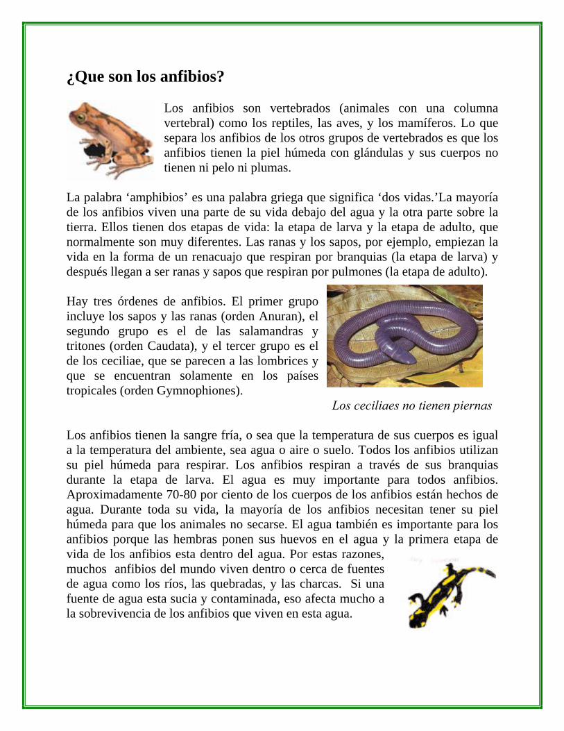
Los anfibios son vertebrados (animales con una columna vertebral) como los reptiles, las aves, y los mamíferos. Lo que separa los anfibios de los otros grupos de vertebrados es que los anfibios tienen la piel húmeda con glándulas y sus cuerpos no tienen ni pelo ni plumas.

La palabra ‘amphibios’ es una palabra griega que significa ‘dos vidas.’La mayoría de los anfibios viven una parte de su vida debajo del agua y la otra parte sobre la tierra. Ellos tienen dos etapas de vida: la etapa de larva y la etapa de adulto, que normalmente son muy diferentes. Las ranas y los sapos, por ejemplo, empiezan la vida en la forma de un renacuajo que respiran por branquias (la etapa de larva) y después llegan a ser ranas y sapos que respiran por pulmones (la etapa de adulto). Hay tres órdenes de anfibios. El primer grupo incluye los sapos y las ranas (orden Anuran), el segundo grupo es el de las salamandras y tritones (orden Caudata), y el tercer grupo es el de los ceciliae, que se parecen a las lombrices y que se encuentran solamente en los países tropicales (orden Gymnophiones). Los ceciliaes no tienen piernas Los anfibios tienen la sangre fría, o sea que la temperatura de sus cuerpos es igual a la temperatura del ambiente, sea agua o aire o suelo. Todos los anfibios utilizan su piel húmeda para respirar. Los anfibios respiran a través de sus branquias durante la etapa de larva. El agua es muy importante para todos anfibios. Aproximadamente 70-80 por ciento de los cuerpos de los anfibios están hechos de agua. Durante toda su vida, la mayoría de los anfibios necesitan tener su piel húmeda para que los animales no secarse. El agua también es importante para los anfibios porque las hembras ponen sus huevos en el agua y la primera etapa de vida de los anfibios esta dentro del agua. Por estas razones, muchos anfibios del mundo viven dentro o cerca de fuentes de agua como los ríos, las quebradas, y las charcas. Si una fuente de agua esta sucia y contaminada, eso afecta mucho a la sobrevivencia de los anfibios que viven en esta agua.

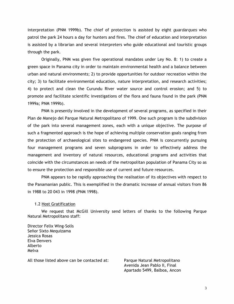
Las ranas y los sapos Las ranas y los sapos son anfibios que tienen piernas posteriores fuertes para saltar rápidamente y piernas delanteras mas cortas. Los ojos de las ranas y de los sapos son grandes para que puedan ver los movimientos en todas las direcciones al mismo tiempo. No obstante eso, las ranas tienen dificultades para ver depredadores y presas que estén cerca de ellos. Los sapos son diferentes de las ranas porque pasan mas tiempo afuera del agua que las ranas. Pero, como las ranas, los sapos tienen que poner sus huevos en agua y en la primera etapa de su vida viven en el agua. Una de las cosas más interesante sobre las ranas es como se cambian de un pequeño huevo para llegar a ser adultos. Los huevos de las ranas se desarrollan en renacuajos que respiran a través de branquias. Esas pequeñas criaturas comen alga en el agua en donde nacieron. Cuando nacen, los renacuajos tienen una cola y una cabeza. Poco a poco, ellos desarrollan piernas. En poco tiempo, llegan a ser adultos con cuatro piernas, sin cola, que comen carne y respiran por los pulmones. La mayoría de los anfibios de Centroamérica nacen de sus huevos en la estación seca cuando hay más insectos que comer.

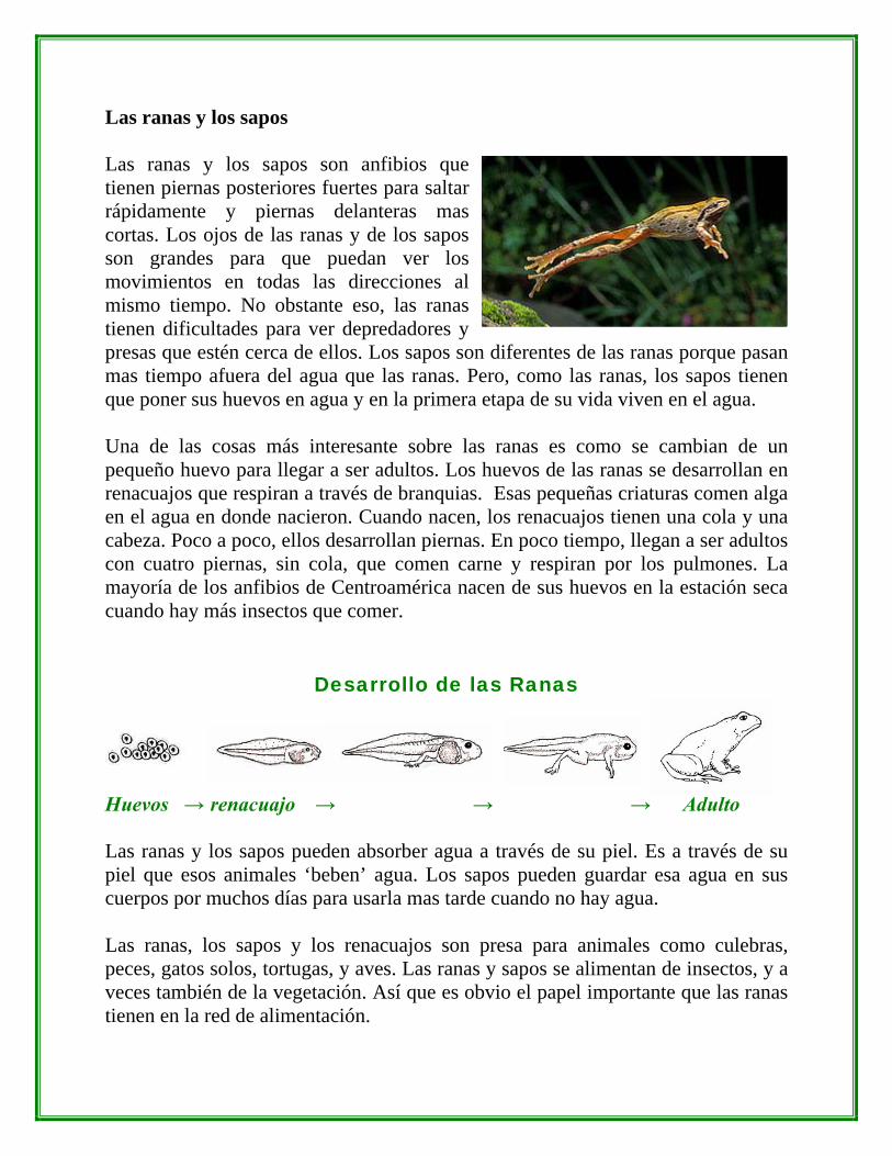
Desarrollo de las Ranas Huevos → renacuajo → → → Adulto Las ranas y los sapos pueden absorber agua a través de su piel. Es a través de su piel que esos animales ‘beben’ agua. Los sapos pueden guardar esa agua en sus cuerpos por muchos días para usarla mas tarde cuando no hay agua. Las ranas, los sapos y los renacuajos son presa para animales como culebras, peces, gatos solos, tortugas, y aves. Las ranas y sapos se alimentan de insectos, y a veces también de la vegetación. Así que es obvio el papel importante que las ranas tienen en la red de alimentación.

Las Diferencias entre las ranas y los sapos

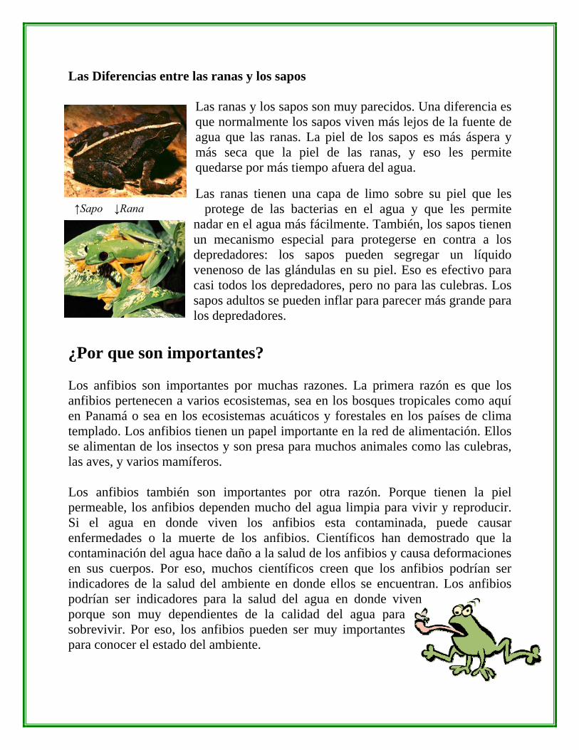
Las ranas y los sapos son muy parecidos. Una diferencia es que normalmente los sapos viven más lejos de la fuente de agua que las ranas. La piel de los sapos es más áspera y más seca que la piel de las ranas, y eso les permite quedarse por más tiempo afuera del agua. Las ranas tienen una capa de limo sobre su piel que les

protege de las bacterias en el agua y que les permite nadar en el agua más fácilmente. También, los sapos tienen un mecanismo especial para protegerse en contra a los depredadores: los sapos pueden segregar un líquido venenoso de las glándulas en su piel. Eso es efectivo para casi todos los depredadores, pero no para las culebras. Los sapos adultos se pueden inflar para parecer más grande para los depredadores.

¿Por que son importantes? Los anfibios son importantes por muchas razones. La primera razón es que los anfibios pertenecen a varios ecosistemas, sea en los bosques tropicales como aquí en Panamá o sea en los ecosistemas acuáticos y forestales en los países de clima templado. Los anfibios tienen un papel importante en la red de alimentación. Ellos se alimentan de los insectos y son presa para muchos animales como las culebras, las aves, y varios mamíferos. Los anfibios también son importantes por otra razón. Porque tienen la piel permeable, los anfibios dependen mucho del agua limpia para vivir y reproducir. Si el agua en donde viven los anfibios esta contaminada, puede causar enfermedades o la muerte de los anfibios. Científicos han demostrado que la contaminación del agua hace daño a la salud de los anfibios y causa deformaciones en sus cuerpos. Por eso, muchos científicos creen que los anfibios podrían ser indicadores de la salud del ambiente en donde ellos se encuentran. Los anfibios podrían ser indicadores para la salud del agua en donde viven porque son muy dependientes de la calidad del agua para sobrevivir. Por eso, los anfibios pueden ser muy importantes para conocer el estado del ambiente.

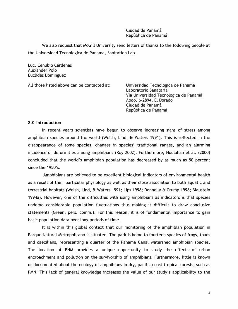
↑Sapo ↓Rana

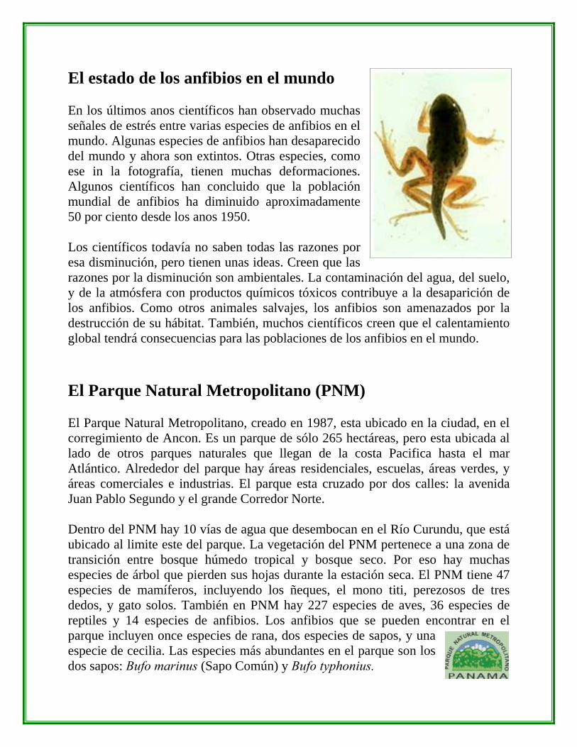
El estado de los anfibios en el mundo En los últimos anos científicos han observado muchas señales de estrés entre varias especies de anfibios en el mundo. Algunas especies de anfibios han desaparecido del mundo y ahora son extintos. Otras especies, como ese in la fotografía, tienen muchas deformaciones. Algunos científicos han concluido que la población mundial de anfibios ha diminuido aproximadamente 50 por ciento desde los anos 1950. Los científicos todavía no saben todas las razones por esa disminución, pero tienen unas ideas. Creen que las razones por la disminución son ambientales. La contaminación del agua, del suelo, y de la atmósfera con productos químicos tóxicos contribuye a la desaparición de los anfibios. Como otros animales salvajes, los anfibios son amenazados por la destrucción de su hábitat. También, muchos científicos creen que el calentamiento global tendrá consecuencias para las poblaciones de los anfibios en el mundo. El Parque Natural Metropolitano (PNM) El Parque Natural Metropolitano, creado en 1987, esta ubicado en la ciudad, en el corregimiento de Ancon. Es un parque de sólo 265 hectáreas, pero esta ubicada al lado de otros parques naturales que llegan de la costa Pacifica hasta el mar Atlántico. Alrededor del parque hay áreas residenciales, escuelas, áreas verdes, y áreas comerciales e industrias. El parque esta cruzado por dos calles: la avenida Juan Pablo Segundo y el grande Corredor Norte. Dentro del PNM hay 10 vías de agua que desembocan en el Río Curundu, que está ubicado al limite este del parque. La vegetación del PNM pertenece a una zona de transición entre bosque húmedo tropical y bosque seco. Por eso hay muchas especies de árbol que pierden sus hojas durante la estación seca. El PNM tiene 47 especies de mamíferos, incluyendo los ñeques, el mono titi, perezosos de tres dedos, y gato solos. También en PNM hay 227 especies de aves, 36 especies de reptiles y 14 especies de anfibios. Los anfibios que se pueden encontrar en el parque incluyen once especies de rana, dos especies de sapos, y una especie de cecilia. Las especies más abundantes en el parque son los dos sapos: Bufo marinus (Sapo Común) y Bufo typhonius.

Los anfibios del Parque Natural Metropolitano

Al limite este del parque esta el Río Curundu, un río muy contaminado por aguas negra y por productos químicos tóxicos que llegan al río de las industrias y empresas que están ubicadas al lado o cerca del río. Esto afecta mucho a las poblaciones de anfibios que viven en el río. También en otras fuentes de agua en el parque, la contaminación y cambios ambientales podrían ser un problema para los anfibios.

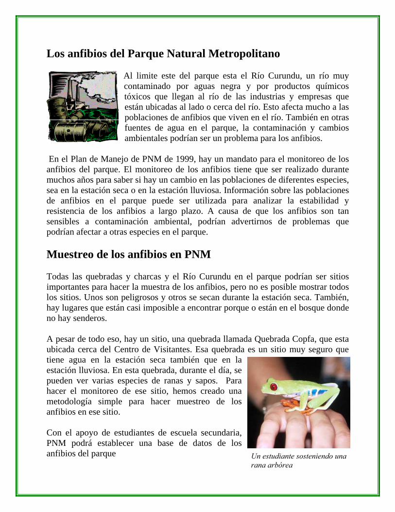
En el Plan de Manejo de PNM de 1999, hay un mandato para el monitoreo de los anfibios del parque. El monitoreo de los anfibios tiene que ser realizado durante muchos años para saber si hay un cambio en las poblaciones de diferentes especies, sea en la estación seca o en la estación lluviosa. Información sobre las poblaciones de anfibios en el parque puede ser utilizada para analizar la estabilidad y resistencia de los anfibios a largo plazo. A causa de que los anfibios son tan sensibles a contaminación ambiental, podrían advertirnos de problemas que podrían afectar a otras especies en el parque. Muestreo de los anfibios en PNM Todas las quebradas y charcas y el Río Curundu en el parque podrían ser sitios importantes para hacer la muestra de los anfibios, pero no es posible mostrar todos los sitios. Unos son peligrosos y otros se secan durante la estación seca. También, hay lugares que están casi imposible a encontrar porque o están en el bosque donde no hay senderos. A pesar de todo eso, hay un sitio, una quebrada llamada Quebrada Copfa, que esta ubicada cerca del Centro de Visitantes. Esa quebrada es un sitio muy seguro que tiene agua en la estación seca también que en la estación lluviosa. En esta quebrada, durante el día, se pueden ver varias especies de ranas y sapos. Para hacer el monitoreo de ese sitio, hemos creado una metodología simple para hacer muestreo de los anfibios en ese sitio. Con el apoyo de estudiantes de escuela secundaria, PNM podrá establecer una base de datos de los anfibios del parque Un estudiante sosteniendo una

rana arbórea

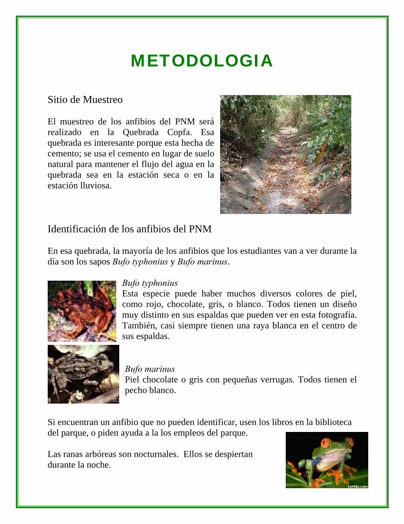
METODOLOGIA Sitio de Muestreo El muestreo de los anfibios del PNM será realizado en la Quebrada Copfa. Esa quebrada es interesante porque esta hecha de cemento; se usa el cemento en lugar de suelo natural para mantener el flujo del agua en la quebrada sea en la estación seca o en la estación lluviosa. Identificación de los anfibios del PNM En esa quebrada, la mayoría de los anfibios que los estudiantes van a ver durante la día son los sapos Bufo typhonius y Bufo marinus.

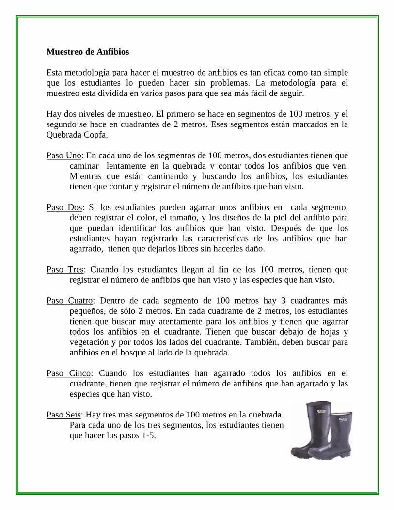
Bufo typhonius Esta especie puede haber muchos diversos colores de piel, como rojo, chocolate, gris, o blanco. Todos tienen un diseño muy distinto en sus espaldas que pueden ver en esta fotografía. También, casi siempre tienen una raya blanca en el centro de sus espaldas. Bufo marinus Piel chocolate o gris con pequeñas verrugas. Todos tienen el pecho blanco.

Si encuentran un anfibio que no pueden identificar, usen los libros en la biblioteca del parque, o piden ayuda a la los empleos del parque. Las ranas arbóreas son nocturnales. Ellos se despiertan durante la noche.

Muestreo de Anfibios Esta metodología para hacer el muestreo de anfibios es tan eficaz como tan simple que los estudiantes lo pueden hacer sin problemas. La metodología para el muestreo esta dividida en varios pasos para que sea más fácil de seguir. Hay dos niveles de muestreo. El primero se hace en segmentos de 100 metros, y el segundo se hace en cuadrantes de 2 metros. Eses segmentos están marcados en la Quebrada Copfa. Paso Uno: En cada uno de los segmentos de 100 metros, dos estudiantes tienen que

caminar lentamente en la quebrada y contar todos los anfibios que ven. Mientras que están caminando y buscando los anfibios, los estudiantes tienen que contar y registrar el número de anfibios que han visto.

Paso Dos: Si los estudiantes pueden agarrar unos anfibios en cada segmento,

deben registrar el color, el tamaño, y los diseños de la piel del anfibio para que puedan identificar los anfibios que han visto. Después de que los estudiantes hayan registrado las características de los anfibios que han agarrado, tienen que dejarlos libres sin hacerles daño.

Paso Tres: Cuando los estudiantes llegan al fin de los 100 metros, tienen que

registrar el número de anfibios que han visto y las especies que han visto. Paso Cuatro: Dentro de cada segmento de 100 metros hay 3 cuadrantes más

pequeños, de sólo 2 metros. En cada cuadrante de 2 metros, los estudiantes tienen que buscar muy atentamente para los anfibios y tienen que agarrar todos los anfibios en el cuadrante. Tienen que buscar debajo de hojas y vegetación y por todos los lados del cuadrante. También, deben buscar para anfibios en el bosque al lado de la quebrada.

Paso Cinco: Cuando los estudiantes han agarrado todos los anfibios en el

cuadrante, tienen que registrar el número de anfibios que han agarrado y las especies que han visto.

Paso Seis: Hay tres mas segmentos de 100 metros en la quebrada.

Para cada uno de los tres segmentos, los estudiantes tienen que hacer los pasos 1-5.

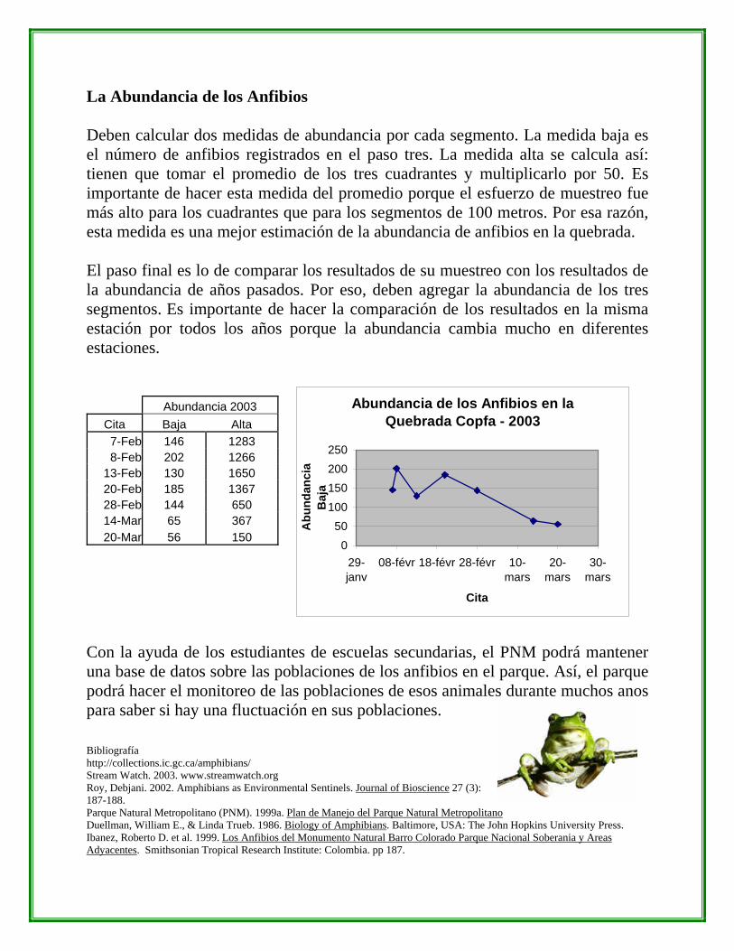
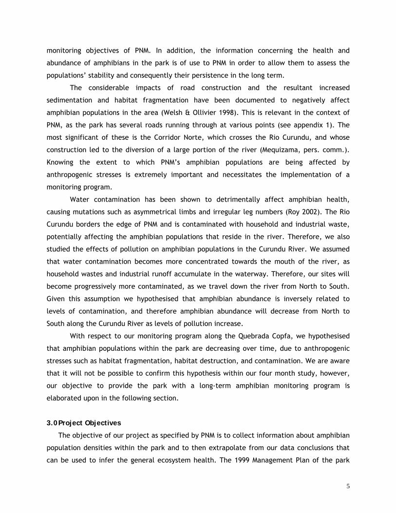
La Abundancia de los Anfibios Deben calcular dos medidas de abundancia por cada segmento. La medida baja es el número de anfibios registrados en el paso tres. La medida alta se calcula así: tienen que tomar el promedio de los tres cuadrantes y multiplicarlo por 50. Es importante de hacer esta medida del promedio porque el esfuerzo de muestreo fue más alto para los cuadrantes que para los segmentos de 100 metros. Por esa razón, esta medida es una mejor estimación de la abundancia de anfibios en la quebrada. El paso final es lo de comparar los resultados de su muestreo con los resultados de la abundancia de años pasados. Por eso, deben agregar la abundancia de los tres segmentos. Es importante de hacer la comparación de los resultados en la misma estación por todos los años porque la abundancia cambia mucho en diferentes estaciones. Abundancia 2003

Cita Baja Alta 7-Feb 146 1283 8-Feb 202 1266

13-Feb 130 1650 20-Feb 185 1367 28-Feb 144 650 14-Mar 65 367 20-Mar 56 150

Con la ayuda de los estudiantes de escuelas secundarias, el PNM podrá mantener una base de datos sobre las poblaciones de los anfibios en el parque. Así, el parque podrá hacer el monitoreo de las poblaciones de esos animales durante muchos anos para saber si hay una fluctuación en sus poblaciones. Bibliografía http://collections.ic.gc.ca/amphibians/ Stream Watch. 2003. www.streamwatch.org Roy, Debjani. 2002. Amphibians as Environmental Sentinels. Journal of Bioscience 27 (3): 187-188. Parque Natural Metropolitano (PNM). 1999a. Plan de Manejo del Parque Natural MetropolitanoDuellman, William E., & Linda Trueb. 1986. Biology of Amphibians. Baltimore, USA: The John Hopkins University Press. Ibanez, Roberto D. et al. 1999. Los Anfibios del Monumento Natural Barro Colorado Parque Nacional Soberania y Areas Adyacentes. Smithsonian Tropical Research Institute: Colombia. pp 187.

Abundancia de los Anfibios en la Quebrada Copfa - 2003

050

100150200250

29-janv

08-févr 18-févr 28-févr 10-mars

20-mars

30-mars

Cita

Abu

ndan

cia

Baj

a

Table of Contents

Executive Summary – English Version i

Executive Summary – Spanish Version ii

1.0 Host Information 1

1.1 Host Institution 1

1.2 Host Gratification 3

2.0 Introduction 4

3.0 Project Objectives 5

4.0 Amphibians as Environmental Indicators 7

5.0 Global Status of Amphibian Populations 8

5.1 Are Amphibian Populations Declining 8

5.2 Potential Factors contributing to Amphibian Declines 10

5.2.1 Climate Change 10

5.2.2 Habitat Modification and Habitat Fragmentation 11

5.2.3 Introduced Species 12

5.2.4 Ultraviolet (UV-B) Radiation 13

5.2.5 Chemical Contaminants and Pollution 13

5.2.6 Acid Precipitation and Soil 14

5.2.7 Disease 15

5.2.8 Trade 15

5.2.9 Synergisms 16

5.3 The Ecological Significance of Amphibians 17

6.0 Methodology 17

6.1 Study Area 17

6.2 Amphibian Sampling 18

6.3 Data Analysis 20

6.3.1 Abundance 20

6.3.2 Quantifying Variables 20

6.3.3 Statistical Analysis 21

6.4 Chemical Analysis of Water Quality 21

6.4.1 Analysis of Dissolved Oxygen using the Winkler Titration Method 22

6.4.2 Calculating Biological Oxygen Demand (BOD) 23

i

7.0 Water Parameters and Effects on Amphibians 23

7.1 pH 23

7.2 Turbidity 23

7.3 Biological Oxygen Demand (BOD) and Dissolved Oxygen (DO) 24

7.4 Total Coliforms 24

7.5 Temperature 25

8.0 Problems Encountered and Sources of Error 25

8.1 Problems Encountered 25

8.2 Sources of Error and Limitations 26

9.0 Results 29

9.1 Quebrada Copfa Project 29

9.1.1 Diversity 29

9.1.2 Seasonal Changes 30

9.1.3 Environmental Factors 30

9.2 The Rio Curundu Project 30

9.2.1 Amphibian Abundance Results 30

9.2.2 Results of Water Quality 32

9.2.3 The Relationship between Amphibian Abundance

and Contamination 33

10.0 Discussion 34

10.1 Quebrada Project 34

10.1.1 Diversity 34

10.1.2 Seasonal Changes 34

10.1.3 Environmental Factors 35

10.2 The Rio Curundu Project 36

10.2.1 Environmental Factors 36

10.2.2 Water Quality 37

10.2.3 The Relationship between Amphibian Abundance

and Contamination 38

11.0 Conclusion and Recommendations 40

12.0 Works Cited 43

Appendix I – Map of Parque Natural Metropolitano 47

ii

Appendix II – Topographical Maps of the Sites Along the Rio Curundu 49

Legend 50

Site 1 51

Site 2 52

Site 3 53

Site 4 54

Site 5 55

Appendix III – Host Product 56

Appendix IV – Raw Data 66

iii

1.0 Host Information

Parque Natural Metropolitano P.O. Box 5499 Balboa, Ancon-Panama Phone: (507) 232 5552 or (507) 232 6723 Fax: (507) 232 5615 Number of full days (8 hours of work) spent on the project: 24 days were spent working on the project. This included research, analysis, writing the final report, working on the host product, and planning out the various presentations. This does not include the days that were spent working in the field. Number of full days spent in the field: 16 days were spent in the field (8hrs per day). This included site surveys and selection, data collection (both night and day), water collection and analysis.

1.1 Host Institution

During the last twenty-eight years Parque Natural Metropolitano (PNM) has evolved to

become Panama’s most distinctive natural areas as it is the only park within all of Central

America to be located within the limits of city. This incredible expanse of land offers visitors,

students, and scientists a unique opportunity to easily access a myriad of habitats ranging

from secondary dry pacific tropical forests to humid tropical rainforests.

In 1974, the 265 hectares of land on which PNM is situated was reforested and

preserved as part of a network of protected areas within the Panama Canal watershed. Prior

to this conversion, the United States’ Armed Forces utilised the land as a training facility for

jungle warfare (Mequizama, pers. comm.). Mandated by a presidential order the Area

Recreativa de Curundú was created in 1983, which was shortly followed by the creation of

PNM in 1985 under Ley No. 8 del 5 de Julio of the Sistema Nacional de Aréas Protegidas

(SINAP). In 1986 the management and administrative structure of PNM was finalised to include

a board of trustees as in accordance with Ley No. 8 (Asemblea Legislativa, 1985). PNM is the

only park in Panama managed in such a fashion. On June 5, 1988, PNM was officially

inaugurated. By 1989, PNM was fully operational with three management units: Protection,

Environmental Education, and Environmental Maintenance (PNM 2002).

The board of trustees is presently composed of representatives from el Municipalidad

de la Cuidad de Panamá (the mayor and legal representation), la Asociación Nacional del

Ambiente (ANAM), la Autoridad de la Region Interoceanica (ARI), la Asociación para la

Investigación y Propagación de las Especies Panameñas (AIPEP, the Smithsonian Tropical

Research Institute (STRI), the Panama Audubon Society, las Asociaciones Civics Unidas (ACU),

and el Club Soroptimista Internacional Panamá-Pacifico (SIPP) (PNM 1998, PNM 2002). The

composition of the board is subject to change depending on the political context and

respective mandates of all organisations involved. It is interesting to note that despite the

presence of numerous governmental agencies on the board of trustees, PNM is a non-

governmental organisation (NGO) entirely dependent on donations.

On the national level, PNM receives regular contributions from the members of the

board of trustees, based on the parks immediate needs and projects. The most important of

these include FIDECO, a sub organisation of both ANAM and Fundación Natura, STRI, and a US$

50,000 trimester annual subsidy provided by the Mayor of Panama City. Unfortunately PNM is

presently suffering from serious financial difficulties due to a cut back this subsidy. Between

1999 and 2002 PNM did not receive US$100 000, a sum critical to the park’s operational

budget and hence the origin of the financial crisis. This crisis was magnified by a similar cut

back in subsidies provided by the private sector as a result of an economic decline in the

country. In 2003, following a series of intense meetings and negotiations, PNM will receive

US$ 50 000 owed to them by the municipal government. However, the remaining amount

owed (US$ 50 000) is to be forgotten as the municipal government has no intention of paying

it. The director of PNM, Señor Felix Wing-Solís, has stated that the park will continue fighting

for what the deserve.

In addition to local funding, International NGOs and corporations such as Texaco,

UNICEF, USAID, Club KIWANIS, and Airbox Express (PNM 1999a) provide funding, thereby

allowing PNM to fulfil projects that extend beyond its regular financial capabilities.

The management and administration of PNM operates under a hierarchical structure,

all of which is overseen by the board of trustees (PNM 1999a). The board of trustees convenes

on a regular basis in order to discuss present and future projects, as well as the park’s

position on various issues. The next division is the Park’s Executive Committee, which consists

of members from both the board of directors and park staff. The committee acts as a liaison

between the board and the park, reporting on all activities and operations, in addition to

managing the financial budget of PNM. The operating executive director of PNM, Señor Felix

Wing-Solís, is responsible for the implementation and maintenance of activities and programs

as specified by the board of trustees and the executive committee. Furthermore, the director

is responsible for overseeing park administration, human resources, and on site management.

The final division in PNM’s management is the administration, which is divided into four

operating bodies: 1) the chief of protection (natural resources); 2) the chief of environmental

and research management; 3) the assistant administrators (including cleaners, secretaries,

drivers, security, accounting, and maintenance; 4) and the chief of education and

2

interpretation (PNM 1999b). The chief of protection is assisted by eight guardarques who

patrol the park 24 hours a day for hunters and fires. The chief of education and interpretation

is assisted by a librarian and several interpreters who guide educational and touristic groups

through the park.

Originally, PNM was given five operational mandates under Ley No. 8: 1) to create a

green space in Panama city in order to maintain environmental health and a balance between

urban and natural environments; 2) to provide opportunities for outdoor recreation within the

city; 3) to facilitate environmental education, nature interpretation, and research activities;

4) to protect and clean the Curundu River water source and control erosion; and 5) to

promote and facilitate scientific investigations of the flora and fauna found in the park (PNM

1999a; PNM 1999b).

PNM is presently involved in the development of several programs, as specified in their

Plan de Manejo del Parque Natural Metropolitano of 1999. One such program is the subdivision

of the park into several management zones, each with a unique objective. The purpose of

such a fragmented approach is the hope of achieving multiple conservation goals ranging from

the protection of archaeological sites to endangered species. PNM is concurrently pursuing

four management programs and seven subprograms in order to effectively address the

management and inventory of natural resources, educational programs and activities that

coincide with the circumstances an needs of the metropolitan population of Panama City so as

to ensure the protection and responsible use of current and future resources.

PNM appears to be rapidly approaching the realisation of its objectives with respect to

the Panamanian public. This is exemplified in the dramatic increase of annual visitors from 86

in 1988 to 20 043 in 1998 (PNM 1998).

1.2 Host Gratification

We request that McGill University send letters of thanks to the following Parque Natural Metropolitano staff: Director Felix Wing-Solís Señor Sixto Mequizama Jessica Rosas Elva Denvers Alberto Melva All those listed above can be contacted at: Parque Natural Metropolitano Avenida Jean Pablo II, Final Apartado 5499, Balboa, Ancon

3

Ciudad de Panamá República de Panamá We also request that McGill University send letters of thanks to the following people at

the Universidad Tecnologica de Panama, Sanitation Lab.

Luc. Cenubio Cárdenas Alexander Polo Euclides Dominguez All those listed above can be contacted at: Universidad Tecnologica de Panamá Laboratorio Sanataria Via Universidad Tecnologica de Panamá Apdo. 6-2894, El Dorado

Ciudad de Panamá República de Panamá

2.0 Introduction

In recent years scientists have begun to observe increasing signs of stress among

amphibian species around the world (Welsh, Lind, & Waters 1991). This is reflected in the

disappearance of some species, changes in species’ traditional ranges, and an alarming

incidence of deformities among amphibians (Roy 2002). Furthermore, Houlahan et al. (2000)

concluded that the world’s amphibian population has decreased by as much as 50 percent

since the 1950’s.

Amphibians are believed to be excellent biological indicators of environmental health

as a result of their particular physiology as well as their close association to both aquatic and

terrestrial habitats (Welsh, Lind, & Waters 1991; Lips 1998; Donnelly & Crump 1998; Blaustein

1994a). However, one of the difficulties with using amphibians as indicators is that species

undergo considerable population fluctuations thus making it difficult to draw conclusive

statements (Green, pers. comm.). For this reason, it is of fundamental importance to gain

basic population data over long periods of time.

It is within this global context that our monitoring of the amphibian population in

Parque Natural Metropolitano is situated. The park is home to fourteen species of frogs, toads

and caecilians, representing a quarter of the Panama Canal watershed amphibian species.

The location of PNM provides a unique opportunity to study the effects of urban

encroachment and pollution on the survivorship of amphibians. Furthermore, little is known

or documented about the ecology of amphibians in dry, pacific-coast tropical forests, such as

PMN. This lack of general knowledge increases the value of our study’s applicability to the

4

monitoring objectives of PNM. In addition, the information concerning the health and

abundance of amphibians in the park is of use to PNM in order to allow them to assess the

populations’ stability and consequently their persistence in the long term.

The considerable impacts of road construction and the resultant increased

sedimentation and habitat fragmentation have been documented to negatively affect

amphibian populations in the area (Welsh & Ollivier 1998). This is relevant in the context of

PNM, as the park has several roads running through at various points (see appendix 1). The

most significant of these is the Corridor Norte, which crosses the Rio Curundu, and whose

construction led to the diversion of a large portion of the river (Mequizama, pers. comm.).

Knowing the extent to which PNM’s amphibian populations are being affected by

anthropogenic stresses is extremely important and necessitates the implementation of a

monitoring program.

Water contamination has been shown to detrimentally affect amphibian health,

causing mutations such as asymmetrical limbs and irregular leg numbers (Roy 2002). The Rio

Curundu borders the edge of PNM and is contaminated with household and industrial waste,

potentially affecting the amphibian populations that reside in the river. Therefore, we also

studied the effects of pollution on amphibian populations in the Curundu River. We assumed

that water contamination becomes more concentrated towards the mouth of the river, as

household wastes and industrial runoff accumulate in the waterway. Therefore, our sites will

become progressively more contaminated, as we travel down the river from North to South.

Given this assumption we hypothesised that amphibian abundance is inversely related to

levels of contamination, and therefore amphibian abundance will decrease from North to

South along the Curundu River as levels of pollution increase.

With respect to our monitoring program along the Quebrada Copfa, we hypothesised

that amphibian populations within the park are decreasing over time, due to anthropogenic

stresses such as habitat fragmentation, habitat destruction, and contamination. We are aware

that it will not be possible to confirm this hypothesis within our four month study, however,

our objective to provide the park with a long-term amphibian monitoring program is

elaborated upon in the following section.

3.0 Project Objectives

The objective of our project as specified by PNM is to collect information about amphibian

population densities within the park and to then extrapolate from our data conclusions that

can be used to infer the general ecosystem health. The 1999 Management Plan of the park

5

calls for an overall monitoring of anuran species and abundance, thus providing the primary

incentive for our project. Furthermore, the Management Plan acknowledges the fact that

amphibians are particularly sensitive to environmental change and can therefore be used as

environmental indicators over time.

The objectives of our project have been defined taking into account that we are

limited by several significant constraints. Principally, it is not possible for us to determine the

long term increase, decrease, or stability of amphibians given that our study is limited to four

months. Secondly, our ability to judge the abundance and diversity of amphibians in the park

is severely limited as only two accessible waterways within the park have water during the

dry season. Furthermore, most sampling must be done during the day, when many amphibians

are not active. Despite these drawbacks, our goal is to give our host institution the tools to

gain more complete information about long term amphibian population trends as well as to

provide a database of population abundance on which future studies can be based.

Our research will focus on two issues. The first was to establish a monitoring program

for the amphibian populations in the Quebrada Copfa. PNM has a severe lack of resources and

cannot employ staff to sample amphibian populations on a yearly basis. However, the park

has important educational facilities that attract students of all ages. Ultimately, our

objective was to establish a program for high school students to work with the park in

sampling amphibians on an annual and voluntary basis. The methodology we used to sample

for frog abundance was simple and inexpensive, the Quebrada Copfa is an accessible, safe

area, and therefore can easily be sampled by untrained volunteers. To facilitate this project,

we designed educational material about PNM’s frogs and toads, and their role as ecological

indicators, in addition to our methodology.

The second study we carried out examined the effects of pollution on the abundance

of amphibians in the Rio Curundu at the park’s eastern boundary. This river is listed as a

critical site under the park’s management plan both because it is isolated from the rest of the

park by the Corredor Norte highway and because it is heavily polluted with household wastes,

industrial effluents, and solid waste. The management plan subprogram for studies on

pollution calls for information about the effects of water pollution at this site. Our objective

was therefore to judge the effects of water contamination on amphibian abundance and

diversity.

In summary, our product will consist of four elements:

1. Baseline data of amphibian abundance and diversity in the Quebrada Copfa

6

2. Educational material about PNM’s amphibians

3. A simple sampling methodology for monitoring amphibians in the Quebrada Copfa

4. A study on the effects of pollution on amphibians in the Rio Curundu

4.0 Amphibians as Environmental Indicators

Despite the fact that amphibian populations across the globe have been decreasing for

about half a century, it is only within the last decade that research has been undertaken by

scientists in an attempt to try and understand how environmental factors and potential

anthropogenic stressors may be affecting the distribution and health of amphibians.

Three aspects of amphibian biology make them sensitive to environmental stress and may

provide insight into understanding the population declines: 1) their permeable skin; 2) their

highly specialized physiological adaptations and specific microhabitat requirements; and 3)

the possession of a complex life cycle, wherein the embryonic and larval stages require

different habitats and foods than adults (Lips 1998; Wake 1990; Blaustein 1994a; Welsh and

Ollivier 1998).

One of the main causal factors cited as responsible for declining populations, is the

special sensitivity that these animals have to toxins and pollutants in the environment (Welsh

and Ollivier 1998; Blaustein 1994a). Amphibians have porous, permeable skin that easily

absorbs chemical contaminants from industrial and domestic waste (Duellman and Trueb

1986). It is because of the increased vulnerability of these animals to even relatively minor

amounts of pollution that amphibians are especially useful as environmental indicators.

Because amphibians are ectothermic animals and possess permeable skin, they must

use behavioural mechanisms to select suitable microhabitat in order to maintain preferable

body conditions (Welsh & Hodgson 1997). This physiological factor becomes relevant when

trying to detect for the effects of habitat change, and the potential effects of global warming

on amphibians.

Amphibians have a complex life history, with both aquatic and terrestrial phases. Most

amphibians live the first part of their life as aquatic larvae and tadpoles that take in oxygen

from the water using gills. Although some amphibians remain aquatic for the duration of their

lives, most amphibians develop into terrestrial, or at least partially terrestrial, animals that

breathe using lungs like other vertebrates (Warkentin 2000). The embryonic and larval stages

of amphibians are susceptible to changes in water quality because of their highly specialized

uses of aquatic habitats for foraging and protection (Welsh and Ollivier 1998). Because of this

specialization and the specific needs, the early life stages of amphibians render them

7

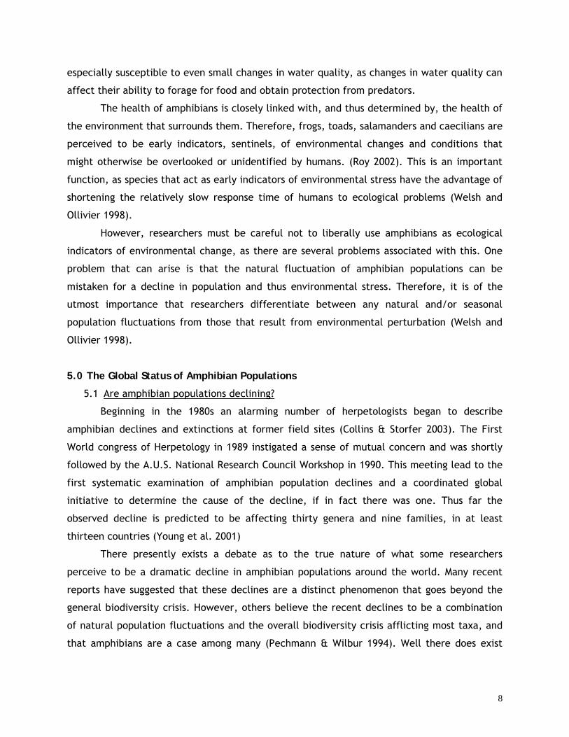
especially susceptible to even small changes in water quality, as changes in water quality can

affect their ability to forage for food and obtain protection from predators.

The health of amphibians is closely linked with, and thus determined by, the health of

the environment that surrounds them. Therefore, frogs, toads, salamanders and caecilians are

perceived to be early indicators, sentinels, of environmental changes and conditions that

might otherwise be overlooked or unidentified by humans. (Roy 2002). This is an important

function, as species that act as early indicators of environmental stress have the advantage of

shortening the relatively slow response time of humans to ecological problems (Welsh and

Ollivier 1998).

However, researchers must be careful not to liberally use amphibians as ecological

indicators of environmental change, as there are several problems associated with this. One

problem that can arise is that the natural fluctuation of amphibian populations can be

mistaken for a decline in population and thus environmental stress. Therefore, it is of the

utmost importance that researchers differentiate between any natural and/or seasonal

population fluctuations from those that result from environmental perturbation (Welsh and

Ollivier 1998).

5.0 The Global Status of Amphibian Populations

5.1 Are amphibian populations declining?

Beginning in the 1980s an alarming number of herpetologists began to describe

amphibian declines and extinctions at former field sites (Collins & Storfer 2003). The First

World congress of Herpetology in 1989 instigated a sense of mutual concern and was shortly

followed by the A.U.S. National Research Council Workshop in 1990. This meeting lead to the

first systematic examination of amphibian population declines and a coordinated global

initiative to determine the cause of the decline, if in fact there was one. Thus far the

observed decline is predicted to be affecting thirty genera and nine families, in at least

thirteen countries (Young et al. 2001)

There presently exists a debate as to the true nature of what some researchers

perceive to be a dramatic decline in amphibian populations around the world. Many recent

reports have suggested that these declines are a distinct phenomenon that goes beyond the

general biodiversity crisis. However, others believe the recent declines to be a combination

of natural population fluctuations and the overall biodiversity crisis afflicting most taxa, and

that amphibians are a case among many (Pechmann & Wilbur 1994). Well there does exist

8

some ambiguity as to the distinctiveness of amphibian declines, they are obviously part of the

general biodiversity crisis, this much is undebatable.

Increasing the complexity of the issue is the fact that amphibian populations are

known to fluctuate, however, there exists limited information on the long-term dynamics of

amphibian populations making it that much more difficult to assess whether present

observations are natural or unusual in magnitude and/or duration. Some studies are available

such as Berven’s (1990) seven year study of Rana sylvatica. This study illustrated that the rate

of population turn over is about two to three years and that populations exhibit erratic

interannual fluctuations largely due to variation in rates of juvenile recruitment. This follows

with Pechmann and Wilbur’s (1994) conclusion claiming that high variability in juvenile

recruitment, including recruitment failures, is commonly observed in amphibian populations

even during short-term studies. Another example is Jaeger’s 14 year study of the Shenandoah

salamander (Plethodon shenandoah) which has been declining and continues to do so as a

result of interspecific competition with P. cinereus, whose population remains stable (Jaeger

1980). Despite the presence of some long-term studies, there are too few to warrant any

sweeping generalisations about the current situation, different species and populations

exhibit specific trends. Furthermore, one should be cautious not to generalise about the

population dynamics of species based on study sites in other regions.

One case which has received much attention as a purported amphibian decline in

Central America is that of the golden toad (Bufo periglenes) of Costa Rica. In 1987, more than

1500 individuals were observed but recruitment was noted to be nearly zero, however, from

1988-1990, only 11 individuals were seen (Crump et al. 1992, in Blaustein 1994a). While it

appears that populations of B. periglenes have plummeted, it is entirely possible that adults

are estivating below ground in response to unfavourable weather conditions, and may emerge

when conditions are more favourable for breeding (Crump et al. 1992, in Blaustein 1994a).

Furthermore, it is known that some species of the same family can live for up to thirty years,

and that many toad species within the same genus can live for up to ten years (Blaustein

1994a). This suggests that B. periglenes can most likely persist under several years of poor

recruitment. The lack of information on B. periglenes’s life history and population dynamics

warrants further study if researchers are to determine the status of the population.

Globally amphibian populations have been declining over the past two decades, but

whether this is a result of population fluctuations, increased monitoring and attention of

amphibians, or a biodiversity crisis is still fervently debated. Most agree that more studies are

needed and that the effort must stem from a sharing of information across a variety of fields

9

not exclusive to herpetology. Empirical evidence suggests a decline of some nature is

occurring, however, the cause is much debated and in fact could be the result of a myriad of

factors interacting to produce the observed result (Collins & Storfer 2003). What alarms

researchers most are the observed declines occurring in what are perceived to be somewhat

pristine locations, devoid of direct human interference.

5.2 Potential factors contributing to amphibian declines

On the basis of studies and observations, a list of factors that may be causing what

some believe to be a substantial decline in global amphibian populations has been created.

This list is in no way exhaustive, however, it does represent what those in the field have thus

far uncovered or believe to be important. According to Young et al. (2001) possible factors

contributing to the decline can be grouped into ten categories: climate change, habitat

modification, habitat fragmentation, introduced species, UV-B radiation, chemical

contaminants, acid precipitation and soil, disease, trade, and synergisms. Determining

whether the reported declines from around the globe have a common cause or whether each

case is site specific with different agents at play is a difficult task, especially when one

considers that amphibians are particularly susceptible to numerous environmental stresses

(Lips 1999). However, one thing is known for certain - human activities are, without a doubt,

causing increased harm to amphibian populations (Pechmann & Wilbur 1994).

5.2.1 Climate Change and Global Warming

It is predicted that climate change and global warming will strongly affect amphibian

populations via four facets: 1) increased temperature; 2) increased length of dry season; 3)

decreased soil moisture; and 4) increased inter-annual rainfall variability (Donnelly & Crump

1998). When considering the ramifications of these changes on amphibian survivorship three

physiological factors are relevant to the discussion: water balance, thermoregulation, and

hormonal regulation of reproduction (Donnelly & Crump 1998). The two processes, which will

be affected most by temperature change as a result of global climate change, are

reproduction and development (Donnelly & Crump 1998). Interestingly, Fetcher et al. (1985)

has documented that despite the fact that daily temperature fluctuations in the Neotropics

are larger than seasonal fluctuations, tropical amphibians appear to show a decreased

capacity for temperature acclimation than their temperate counterparts. Therefore, it is

entirely plausible that with changes in ambient temperature we will see a parallel shift in

species’ geographic distributions (Carey & Alexander 2003). Furthermore, a warmer and drier

10

climate may be an environmental stress conducive to immuno-suppression of amphibians thus

making them more susceptible to infectious disease and death (Crawshaw 1992, in Donnelly &

Crump 1998).

Donnelly and Crump (1998) have made several predictions, based on their knowledge

and observations, on how leaf-litter and pond-breeding anurans will be affected by changes in

climate. Firstly, with respect to leaf-litter anurans, they believe that in a warmer, drier, and

less predictable climate a change in food supply will occur. If prey population sizes decrease,

juvenile frogs will experience decreased growth rates and adults may allocate less energy to

reproductive functions. The latter would result in decreased clutch size, egg size, and/or

clutch frequency. In addition, a decrease in soil moisture may potentially lead to problems of

water imbalance for many anuran species that rely on direct development and deposit their

eggs in the leaf litter (Donnelly and Crump 1998). Secondly, climate change is expected to

have major consequences for pond breeding anurans as their ability to accumulate nutrients

and energy for reproduction may be hindered as a result of changes in the invertebrate prey

base (Donnelly and Crump 1998). Furthermore, unpredictability of rainfall patterns, increased

length of dry season, and lower humidity will result in timing problems for bond breeders as

well as harsher environmental conditions for those eggs deposited on leaves above the water

(Donnelly and Crump 1998). They conclude that sporadic breeders will be the least affected

by climate changes that alter pond hydrology, and that explosive breeders will not be

affected as seriously as prolonged breeders as they are already adapted to accomplishing

reproduction in a relatively short period of time, under conditions of high density.

Herpetologists have predicted that those amphibian populations at the edges of their

distributional ranges will be especially vulnerable to local and global climate changes as it is

in these areas that the effects of temperature change will be most acutely felt (Carey &

Alexander 2003). With respect to Neotropical amphibians, those species which have narrow

endemic ranges will be the most affected by climate change (Donnelly & Crump 1998). The

supposed disappearance of B. periglenes in Costa Rica is believed to be an example of this

type of vulnerability based on a limited geographical distribution (Donnelly & Crump 1998).

5.2.2 Habitat Modification and Habitat Fragmentation

Amphibian diversity is known to be severely threatened by habitat destruction and

habitat alteration as they are undoubtedly the single most important cause for declines of

species in all taxa (Blaustein 1994a). Human practices such as forest clearing for settlement

and agriculture, as well as the draining of wetlands and bogs are known to be particularly

11

deleterious for not just amphibian populations, but all organisms (Young et al. 2001). These

consequences extend beyond just the fracturing of population dynamics, to the facilitation of

local and regional extinction of populations and species by killing organisms, removing

habitat, or preventing access of animals to breeding sites (Collins and Storfer 2003).

Furthermore, Sedimentation of streams and rivers, is a common outcome of many land

management activities such as logging, mining, and grazing, in addition to road construction

(Meehan 1991, in Welsh & Ollivier 1998). Welsh & Ollivier (1998) found that amphibian

densities in North-western California were significantly lower in streams that were impacted

by sedimentation, and that all species proved to be vulnerable to sedimentation due to their

common reliance on interstitial space in streambeds for critical life requisites such as

foraging and breeding.

Habitat fragmentation can result from habitat destruction, construction of roads,

introduced species, and low pH in some areas, thus creating barriers to dispersal. In PNM the

construction of the Corridor Norte, a four lane highway, and a set of electrical wires, which

have allowed Saccharum spontaneum to establish itself in the park, have resulted in the

division of the park into two parts. The consequences of this fragmentation in such a small

forested space on amphibian populations, are yet to be observed and documented, however

our study attempts to shed light on this.

5.2.3 Introduced Species

Alien species often cause declines and even extinctions of native amphibian

populations through a variety of mechanisms, acting alone or in concert (Collins & Storfer

2003). These include predation by alien species on native amphibians, direct and indirect

competition between one or more life stages, the introduction of pathogens by non-natives

and hybridisation. (Collins & Storfer 2003). One well documented example is that between

Rana muscosa, a native of the Sierra Nevada Mountains (USA), and an introduced trout species

which has been responsible for the decline in amphibian populations and the possible

disruption of amphibian metapopulation structure (Knapp et al. 2001, in Collins & Storfer

2003; Pilliod & Peterson 2001, in Collins & Storfer 2003). By 1910, R. muscosa had

disappeared from virtually every lake where the invasive trout species had been stocked

(Vredenburg 1998). In Latin America introduced plant and animal species such as pine,

eucalyptids, salmonids, and bullfrogs are believed to be a threat to amphibian populations

(ECOSUR,STRI,PUCE 1999). However, according, to Lips (1998) those amphibians which occupy

forest pools, bromeliads, and other isolated bodies of water are safe from trout predation. In

12

PNM, the non-native invasive grass species Saccharum spontaneum is of particular concern

among park officials, as the long term effects of the grass on the native flora are unknown.

Therefore, officials cannot predict how it will affect amphibian populations (Mequizama 2003,

pers. comm.)

5.2.4 Ultraviolet (UV-B) Radiation

It is a well established fact that natural events such as solar flares can cause increases

in UV radiation, however, it is also known that the current increases in levels of UV radiation

are a result of anthropogenic abuses upon the ozone, such as chlorofluorocarbons (CFCs) and

other chemicals that deplete stratospheric ozone layer (Storfer 2003). Furthermore, Kerr and

McElroy (1993) have shown that levels of UV radiation have risen significantly both in

temperate areas and in the tropics over the past two decades. As a result, like all organisms,

amphibians encounter increasing levels of UV radiation. However, this increase in UV-B

exposure happens to coincide with many of the observed amphibian declines, causing some to

examine whether causality between the two variables can be established (Blaustein et al.

1994b, 2003; Kiesecker et al. 2001). The effects of UV radiation on amphibian populations

depends on a number of variables, including the length and level of exposure, sensitivity and

ecological factors, all of which vary between regions and species (Kiesecker 2001).

When living organisms, including amphibians, absorb UV-B radiation at levels above

their critical tolerance capabilities irreparable damage can result. UV radiation, either alone

or in concert with other toxins in the environment, has shown to cause immune dysfunction,

altered behaviour of amphibians, slower growth rates and retarded development, limb

malformations, and death (Blaustein et al. 2003). Furthermore, exposure to UV-B radiation

can induce subleathal effects in embryos, larvae, and adults, and in some extreme cases can

result in death depending on species and life stage (Biek et al. 2002; Blaustein et al. 2003). In

addition, UV-B radiation can also contribute to retinal damage, lesions, and increased

susceptibility to diseases and low pH (Young et al. 2001).

5.2.5 Chemical Contaminants and Pollution

Many environmental contaminants (agrochemicals, industrial pollution, and heavy

metals) accumulate in sediments and water, in addition to vaporising readily making them

easily transportable over long distances in the atmosphere. Furthermore, pesticides,

herbicides, and chlorinated hydrocarbons have permeated the landscape and are extremely

persistent. This is particularly hazardous and prevalent to amphibian survivorship as these

13

chemicals can kill anurans directly and/or result in developmental and behavioural

abnormalities thus propelling a decline in the population (Lips 1999; Blaustein et al. 2003).

Few studies have documented the effects of pesticides on amphibians under natural

conditions, however, the effects of DDT and organophosphate pesticides are know to be

lethal as both have contributed to population declines (Blaustein et al. 2003).

Heavy metal contamination can also result in developmental abnormalities as well as

increased metabolic rates, which could indicate a physiological cost to exposure of

contaminants (Blaustein et al. 2003). Another hazardous chemical acting on amphibians is

that of nitrogen pollution from anthropogenic sources. Nitrates enter aquatic systems via

agricultural runoff and/or percolation into groundwater, from where they come into direct

contact with amphibians. Studies show that nitrogenous contaminants can reduce feeding

activity and swimming behaviour, and result in certain malformities and death in some

species of Anura (Blaustein et al. 2003). Furthermore, some chemical contaminants, such as

CFCs and atrazine, can act as endocrine disrupters thereby affecting reproduction in

amphibian populations and instigating a decline (Gendron et al. 1997, in Blaustein et al.

2003).

5.2.6 Acid Precipitation and Soil

Exposure to increased levels of pH has become more of a problem over the last few

decades as a result of increased pollution leading to acid rain and the acidification of aquatic

systems by toxins. As a result these systems are uninhabitable for many species, thereby,

dramatically reducing biodiversity. In the tropics, acidification is problematic because many

tropical soils are acidic (Lips 1998). Because stream water must percolate through and across

the soil, numerous tropical montane streams and ponds have become acidic over time (Lips

1998). Acidification also leads to the leaching of heavy metals, such as aluminium, from the

soil into the water column (Beattie 1990).

The effects of acid exposure on developing frogs are known to include decreased

sperm motility, high mortality, and developmental abnormalities in embryos and tadpoles

(Simon et al. 2002; Bradford & Gordon 1995; Beattie and Tyler-Jones 1992; Sadinski and

Dunson 1992). The anuran families Hylidae, Ranidae, and Bufonidae have exhibited

reproductive problems below pH 5.0 (Sparling 1995, in Lips 1998). Furthermore, a few studies

have shown that exposure to conditions of a pH below 4-5 may cause death by disrupting ion

transport through the skin (Lyall et al. 1992, in Simon et al. 2002). All species of amphibian

exhibit different levels of tolerance to acidic conditions and thus the causal relation between

14

low acidity and population decline is species dependent. For example, Rana pipiens, when

exposed to a pH of 5.5 experienced 72 percent mortality, however, Bufo marinus did not

exhibit reduced immune competence when exposed to pH 3.8 for 14 days (Simon et al. 2002).

5.2.7 Disease

Emerging infectious diseases are now being recognising as a significant direct cause for

amphibian declines, particularly in relatively isolated and untouched areas. Several pathogens

are suspected and have been isolated, the first of which a chytrid fungus, Batrachochytrium

dendrobatidis. B. dendrobatidis has been associated with anuran declines and extinctions in

Australia, North America, and Central America (Collins & Storfer 2003; Lips 1998, 1999). The

distinguishing factor of B. dendrobatidis is that it is also found to co-exist with non-declining

species in the same area, thus making all wild amphibians potential pathogen reservoirs, with

species specific rates of survivorship (Collins & Storfer 2003). Lips (1998, 1999) has reported

and documented on two cases of amphibian decline in Central America, the first in Costa Rica

and the second in Panama, for which she believes the chytrid fungus is responsible. Lips

(1999) speculates that the pathogen which caused the declines in Monteverde, Costa Rica is

the same as that which caused mass mortality in Fortuna, Panama. Another fungal pathogen

believed to be responsible for declines in North America is Saprolegnia ferax (Kiesecker et al.

2001; Carey & Alexander 2003).

The second major group of infectious disease suspected is the iridovirus (Collins &

Storfer 2003). However, long term studies on salamanders suggest that unlike the mass

declines associated with fungal epidemics, iridoviruses may simply cause population

fluctuations (Collins et al. 1998, in Collins & Storfer 2003). Two strains of iridovirus/ranavirus

have been isolated so far in North America. Because both pathogens, fungal and iridovirus,

exhibit different roles with respect to amphibian population dynamics, it is hypothesised that

iridoviruses have coevolved with amphibians as population most often recover after 1 to 2

years (Collins & Storfer 2003).

5.2.8 Trade

The international amphibian trade for culinary, pet, medicinal, and biological supply

markets has been operational for more than a century (Young et al. 2001). As early as the

1970s, suppliers in North America had noticed a decline in certain amphibian species, thus

making a connection between harvesting and declining amphibian populations (Collins &

Storfer 2003). Although harvesting of amphibians is not the largest or most important factor,

15

it can be significant, as shown by Lanoo et al. (1994, in Collins & Storfer 2003). They

estimated that between 1920 and 1992 amphibian populations in one Iowa county, USA,

declined from approximately 20 million frogs to 50 000, of which one third of the decline can

be attributed to harvesting, and the remaining to the drainage of wetlands.

5.2.9 Synergisms

Synergism, is the term used to describe the phenomenon of various factors working

together to attain one outcome, within this context that outcome is the mortality of and

sublethal effects on amphibian populations. As several studies would suggest it is the

combination of several of the above factors, working in cohort, which is responsible for the

perceived decline as one stress makes amphibians more susceptible to other stresses (Carey

1993; Lips 1998; Lips 1999; Collins & Storfer 1998; Kiesecker et al. 2001). Lips (1999) has

observed that in the tropics all unexplained amphibian declines have occurred in upland

areas, thus suggesting that the cause has a synergistic interaction with some environmental

condition(s) that varies with elevation such as temperature, wind patterns, ultraviolet (UV-B)

radiation, or precipitation.

With respect to alien species, studies have shown that in addition to directly affecting

amphibian populations through competition and predation, they can also interact with a

variety of other factors, such as acting as a vector for infectious diseases which can lead to

complex and indirect effects (Collins & Storfer 1998). In addition, amphibians exposed to low

pH and/or high UV-B radiation may experience immuno-suppression followed by microbial

diseases resulting in mortality (Carey 1993; Lips 1998; Lips 1999; Kiesecker et al. 2001).

Furthermore, climate induced reductions in water depth at oviposition sites have causes high

mortality of embryos by increasing their exposure to UV-B radiation and thus making them

more susceptible to infection (Kiesecker et al. 2001).

Regarding environmental contaminants, studies have shown that inorganic monomeric

aluminium often acts synergistically with pH to cause embryo mortality and deformity in

amphibians (Beattie 1992; Bradford et al. 1992; Blaustein et al. 2003). Given the fact that a

myriad of synergistic relationships between the above mentioned factors exist, it is extremely

difficult for researchers to isolate and/or uncover one particular mechanism. This ambiguity

necessitates the need for future study of these factors, with relation to amphibian population

in order to solve the mystery of what is causing amphibian declines.

5.3 The Ecological Significance of Amphibians

16

Why should we care that global amphibian populations are declining at what some

believe to be an alarming rate that may lead to widespread extinctions? We should care

because amphibians are central components in many communities and food webs (Donnelly &

Crump 1998). The intricate life cycle (terrestrial and aquatic phases) of many amphibian

species results in greater ecological complexity as different life history stages participate in

different food webs (Duellman & Trueb 1986). Thus, changes in density at each life history

stage will have serious ramifications for not only all other elements within their respective

food web but also on other food webs in which other life history stages engage.

In a forest ecosystem up to 90 percent of the net primary production enters the

detritus based food web, thus making it closely involved with energy flow and nutrient cycling

(Chen & Wise 1999). The path by which this energy becomes available to higher trophic levels

is mainly through arthropod - amphibian interactions as they are the link between below

ground and above ground food webs (Chen & Wise 1999). In an aquatic system, anuran

tadpoles are generally herbivorous, consuming vast quantities of algae, and as such tadpoles

play an important role in the transfer of nutrients between the aquatic and terrestrial

environments (Seale 1980, in Donnelly & Crump 1998). Is it not than a possibility to observe

increased rates of eutrophication if tadpole numbers radically decline? Contrarily might we

not experience outbreaks of arthropods normally preyed on by amphibians or decreased

densities of those vertebrates that prey on amphibians?

Despite the ecological importance and diversity of amphibians living in a myriad of

habitats, they are generally not considered in discussions of ecosystem function (Dunsun et al.

1992; Drost and Fellers 1996, in Donnelly & Crump 1998). However, many researchers

speculate that if global populations are truly declining, than the consequences will cascade

throughout the system, negatively affecting many animals. It is for this precise reason that so

many individuals are scrambling to accurately determine the state of amphibian populations

and the potential factors that are causing their perceived decline.

6.0 Methodology

6.1 Study Area

Our sampling strategy was developed for and tested in the waterways of Parque

Natural Metropolitano (PNM) in Panama City, Panama. PNM is a national park within the limits

of the city of Panama that covers a total area of 265ha. The locations of the sampling sites in

PNM enabled us to formulate two projects, the first being the establishment of baseline data

for amphibian populations in the park, and the second being the study of the effects of urban

17

settlement and water pollution on amphibian. The sampling was undertaken in the dry

season, during the months of January, February, and March.

Two waterways were sampled in order to carry out the objectives of our project. The

first of these waterways is the Copfa Stream (Quebrada Copfa), located in the centre of the

park. This stream is unique in that its bottom has been lined with concrete so as to maintain

water flow throughout the year, including the dry season. The concrete is a necessary

addition to the maintenance of water flow, as is evidenced by the fact that it is both the only

paved stream in PNM and the only stream in the park that maintains water flow during the dry

season. The second waterway that was sampled is the Curundu River, which borders the

eastern edge of PNM and flows from North to South. We also tested water quality at sites 1,

4, and 5 along the Curundu, to gage the effects of water quality on amphibians.

6.2 Amphibian Sampling

In order to carry out our sampling of amphibians in PNM we modified the sampling

technique used by Welsh, Hartwell and Hodgson (1997) in order to reflect our particular needs

and study area.

Our approach integrated a 3-tiered riparian/aquatic and upland sampling strategy that

was applied to five, 100 meter segments in the Curundu River and three, 100 meter segments

in the Copfa Stream. These 100 meter segments (one segment will be referred to as a

transect hereafter) comprised the primary unit of analysis for our study. The transects also

denied the spatial limitations of our sampling. The transects that we sampled were intended

to be representative of pre-selected sites within the waterways that were selected based

upon our perception and initial qualitative analysis of water quality and upland vegetative

growth. The placement of each transect within each waterway was determined randomly.

Randomness was ascertained by drawing a random number between 1 and 100, and then

pacing that distance in meters from the point where an access trail or road first met or

crossed each waterway. Due to the difficulties of accessing one site along the Curundu River

(Site 5), the placement of this site was slightly modified in order to render it accessible.

The selection and sampling of each transect was carried out during the dry season

only. Sampling during this season was facilitated by a lack of rainfall and ambient moisture,

therefore many amphibians were aggregated in the waterways of the park in which we

sampled. All of the transects that we sampled in the Curundu River were perennial, as water

was present in these areas both during the wet and dry seasons. In the Copfa Stream,

however, only two of the three transects retained water throughout the dry season.

18

In the Copfa Stream, we had three transects of 100 meters in which we monitored

amphibian abundance over a period of 2 ½ months. In all three of these transects we sampled

a total of seven times during the day and once during the night (in order to compare

differences in amphibian activity for day and night times, as well as to give a better total

estimate of amphibian density in the stream). In the Curundu River we sampled a total of five

transects, four of which were upstream of the major sources of contamination of the river.

More transects were not sampled further downstream in the more contaminated areas of the

river because of the river's inaccessibility. We sampled each of the five sites on the river

three times during the course of our study.

Tier 1

The first tier, a distance based visual encounter sample technique, was conducted

with two people walking slowly upstream from the south end of the belt to the northern end.

One person watched for animals in the water and on the streambed and streamside substrates

and recorded their observations. The second person, using a measuring tape, mapped the

topography of the stretch and the location of seeps, springs, and side channels as well as

substrate composition and presence of rocks or islands. The pair also classified the transect

according to habitat, vegetation cover, and rate of water flow. The maps included distances

as well as landmarks. The rate of water flow was determined qualitatively by observing the

relative velocity of water flow, and was assigned a rank (stagnant, slow, medium, or fast).

For visual representations of these maps refer to Appendix II.

Tier 2

The second tier of sampling consisted of area-constrained searches (ACS) of three, 2m

belts, which were randomly chosen within each 100m transect. The randomness of belt

locations within each transect was ascertained by subdividing the 100m transect into fifty 2m

sections and then and then drawing a number between 1 and 50. The number that was chosen

at random dictated the location of the 2m belt in which we performed the ACS. For example,

if the number 16 were chosen then the area between 32 and 34 meters would be the belt of

the ACS. At times the placement of the 2m belt was adjusted slightly up or down stream if

necessary in order to avoid working in thick vegetation where observations would be severely

hampered. Each 2m belt was sampled from downstream to upstream in order to avoid

disturbing the amphibians in the transect that had not yet been sampled. We used a small

fishnet in order to capture all the amphibians that were found in each belt. This was done in

19

order to avoid recapturing the same individuals. The animals were released immediately after

the ACS sampling was finished in each 2m belt. In order to provide information on

microhabitat associations we measured belt width, mean water depth, substrate composition,

and average water velocity. Tier 2 was not performed at site 5 as we were not able to get

into the water due to health and safety risks.

Tier 3

The third tier of sampling consisted of a 30 minute constrained search in any spring,

seep, or pond that was present along the 100m transect. If there were no springs or ponds

present along the 100m transect then no third tier sampling was conducted.

6.3 Analysis of Data

6.3.1 Abundance

We calculated two measures of amphibian abundance. The low measure is simply the

number of frogs observed in the first tier of sampling, and the high measure is the average of

the number of frogs sampled in each 2m belt during the second tier, multiplied by a factor of

fifty in order to estimate the total abundance of the 100m transect. Assuming that the

randomly selected belts are representative of the transect, the high estimate is a more

accurate measure of abundance because each belt was scrutinized with greater effort than in

tier 1 sampling, and all frogs were captured and counted. However, because we were unable

to perform tier 2 at site 5, the analysis of the Rio Curundu was restricted to the use of tier 1

data. Furthermore, for site 5, we were only able to sample along an 80m transect, therefore,

we multiplied the abundance by 1.25 in order to be able to compare it to the other 100m

transects.

6.3.2 Quantifying variables

Environmental variables, such as leaf litter and rate of water flow were assessed

qualitatively at each belt. In order to analyze the effects of these environmental factors, they

were quantified in the following manner:

- Leaf litter: 1 = little or minimal; 2 = medium; 3 = lots - Flow: 0 = no water, 1 = stagnant or very slow, 2 = slow, 3 = medium, 4 = fast - Foliage cover: 1 = 0-24% shade, 2 = 25-49%, 3=40-74%, 4= 75-100% - Presence of tadpoles was quantified as 1 while absence of tadpoles was quantified as 0. - pH was quantified as the difference from a neutral pH of 7.0, so that a pH of 6 or 8 would

both be quantified as 1.

20

Diversity was calculated in terms of species richness and Simpson Index. The Simpson

Index was selected because it is independent of sample-size, which was necessary as we had

only one night sample to compare to seven day replications. The Simpson Index is 1/∑p2

where p is the proportional abundance, calculated as the number of individuals of a given

species divided by the abundance.

6.3.3 Statistical Analysis

As the abundance values were not normally distributed, a Kruskal-Wallis non-

parametric test was used to determine whether there was a difference in abundance between

transects in each water system. A linear regression was used to detect trends in abundance

over time. In order to determine the relationship between amphibian abundance and various

environmental factors in the Quebrada Copfa, correlations were made using data collected

from tier 2. Correlations were also made between the presence or absence of tadpoles and

abundance of adults, as well as various environmental factors. A t-test was used to determine

whether differences in diversity between day and night were significant. In order to

determine the causality of water quality on amphibian populations regressions, correlations,

and spearman rank correlations were drawn between water quality and low abundance

estimates in sites 1, 4 and 5. Low abundance estimates were used because high estimates

were not available for site 5. Data was log-transformed when it was not normally distributed.

6.4 Chemical Analysis of Water Quality

The water quality analysis was carried out for three of the five 100m stretches along

the Curundu River. The collected water from the topmost site (Site 1) of the river, the site in

which the largest number of frogs were found (Site 4), and the most contaminated site along

the river (Site 5). A total of two litres of water was collected at each of the three sites. The

water samples were kept cold during the transportation from the river to the university lab

using a cooler filled with ice. We noted and recorded observations concerning the external

quality and contamination of the river. At each of the three sites we tested the following

chemical and biological parameters:

1. pH 2. turbidity 3. BOD5 (biological oxygen demand) 4. DO (dissolved oxygen) 5. total coliforms 6. temperature

21

NB - All parameters except temperature were analysed in the Sanitation Lab at the Universidad Tecnologica de Panamá.

In order to determine the concentration of dissolved oxygen and the biological demand

of oxygen of each water sample we employed the Winkler Titration Method.

6.4.1 Analysis of Dissolved Oxygen using the Winkler Titration Method

Dissolved oxygen analysis measures the amount of oxygen, in its gaseous state, that is

dissolved in a solution.

1. For each sample of water, 5 dilutions must be carried out. We used dilutions of 100 percent (no dilution), 0.5 percent, 1 percent, 2 percent, and 5 percent. There must be 2 bottles of each dilution.

2. Fill each bottle half way with oxygenated water. 3. In each pair of bottles add:

1. 1mL of Iron (III) chloride 2. 1mL of Buffer 3. 1mL of Magnesium sulphate 4. 1mL of Calcium chloride

5. Fill both of the bottles to the top and seal them with the stopper. 6. With the first bottle, seal the top with aluminium foil and place in the incubation area

at 20ºC, for 5 days in order to measure BOD. 7. In the second bottle, unstopper it and pipette the following:

1. 2mL of Manganous Sulfate 2. 2mL of Alkaline Potassium Iodide Azide

8. Recap the bottle and shake several times. 9. Let the bottle stand until precipitate has fallen to the halfway point of the bottle. 10. Add 2mL of Sulfuric Acid. 11. Recap the bottle and invert bottle until precipitate dissolves. 12. Using a graduated cylinder, measure 200mL of solution from the bottle. The solution

will be orange in colour. 13. Titrate this 200mL with Sodium Thiosulfate until the solution turns from an orange

colour into a pale yellow. 14. Add a drop of indicator so that solution becomes dark blue. 15. Titrate with Sodium Thiosulfate until solution becomes totally clear. 16. Record the amount of Sodium Thiosulfate that was used in both steps of the titration -

this number is the amount of Dissolved Oxygen in mg/L in the water.

The ANZECC Guidelines (1992) recommend that for the protection of freshwater systems,

levels of dissolved oxygen should not fall below 80-90 percent saturation. Levels of dissolved

oxygen that are below 2mg/L do not support fish life, and levels below 3mg/L are stressful to

most aquatic organisms, including amphibians. Levels of 5-6mg/L are necessary in order to

support minimal growth and activity of aquatic organisms.

6.4.2 Calculating Biological Oxygen Demand (BOD)

Biological Oxygen Demand is a measure of the amount of oxygen that has been

22

consumed by biological processes over a period of 5 days.

1. After a 5 day incubation period, remove the bottles from the incubator. 2. Perform the Winkler Titration Method, step 7 to 16, in order to determine the amount

of dissolved oxygen present in these bottles. 3. Calculate the BOD by subtracting the amount of dissolved oxygen remaining after the

5 day incubation period from the mg/L of dissolved oxygen measured on day 1. NB - The difference in levels of dissolved oxygen between day 1 and day 5 is the BOD, or the consumption of dissolved oxygen by biological processes over that 5 day period. Unpolluted waters will have a BOD of 5mg/L or less. Raw sewage can have BOD levels of

150mg/L to 300mg/L or higher.

7.0 Water Parameters and Effects on Amphibians

7.1 pH

The parameter of pH is a measure of the concentration of hydrogen ions in the water.

A pH of 7 indicates that the water is neutral, neither acidic nor basic. Values below 7 indicate

that the water is increasing in acidity, and values above seven indicate that the water is

increasing in basicity. Fresh water is usually slightly basic as a result of the presence of

carbonates and bicarbonates in the water. The acceptable level of pH for fresh water systems

is a pH 6.5-9 (Environment Canada 1999) and should be such in the Curundu River.

7.2 Turbidity

Turbidity is a parameter used to measure the clarity of water. The greater the amount

of suspended solids in the water, the hazier it appears and the higher will be its turbidity

value. Turbidity is generally caused by particles of clay, silt, and sand, as well as

phytoplankton, bits of vegetation, industrial wastes, and sewage (Duluth Streams 2003).

Therefore, it is possible to use this parameter to measure the presence of industrial and

domestic effluents in the water. The Environmental Protection Agency (EPA) of the United

States has identified siltation as the most important source of water quality degradation

(Henley et al. 2000). Acceptable values for turbidity of fresh water are less than 5 NTU, as

outlined by ANZECC, the Australian Water Quality Guidelines for 1992. Cenobio Cárdenas, a

professor of chemistry at the Universidad Tecnologica de Panama, confirmed this value of 5

FAU.

7.3 Biological Oxygen Demand (BOD) and Dissolved Oxygen (DO)

The term dissolved oxygen (DO) refers to the amount of free oxygen that is dissolved

23

in the water and available to aquatic organisms. Oxygen diffuses into aquatic systems in a

number of different ways: via aeration from the atmosphere, by movement of currents and

ripples in the water, and as a waste product of photosynthesis. In a stable system, oxygen is

replenished as quickly as it is used. The minimum amount of dissolved oxygen that is

necessary for the survival of aquatic life is 5mg/L (Cárdenas, pers. comm.).

In this study, the term biological oxygen demand (BOD) is an empirical measure of the

amount of dissolved oxygen used by micro-organisms in the water to assimilate organic wastes

over a period of five days. In other words, BOD tells us how quickly the available dissolved

oxygen is being consumed by micro-organisms and by chemical processes in the water. In

streams that are very polluted with sewage and industrial waste, the BOD will be very high as

micro-organisms use oxygen to assimilate the organic matter. If BOD is too high, this can

leave little available dissolved oxygen for other aquatic organisms such as amphibians. As

stated by Stream Watch (2003), the results of BOD analysis can be used to evaluate the

impact of organic material and eutrophication on water quality.

There is an inverse relationship between levels of BOD and DO in water, signifying that

as eutrophication increases, presence of DO decreases. Furthermore, excessive contamination

of waterways by industrial or domestic organic waste products result in high levels of BOD and

low levels of DO, thus having negative impact on aquatic organisms, including amphibians.

7.4 Total Coliforms

The measurement of total number of coliforms present in water is extremely

important as it provides a means to assess the quantity of raw sewage that is deposited

directly and indirectly into the Curundu River. According to international norms, the

maximum quantity of faecal and other coliforms permissible in water that is to support

aquatic wildlife is 10 000 coliforms per 100mL (PMCC, 1999).

Faecal coliforms are micro-organisms that colonize the large intestines of warm-

blooded animals and are excreted in faeces. Faecal coliforms can enter streams and rivers via

sewers and septic systems, runoff from storm water carrying animal faeces, from intensive

farming, and from waterfowl and livestock defecating in or near the water. The presence of

faecal coliform in water is an indication of the presence of other, more potentially dangerous

pathogens in the system as well.

7.5 Temperature

24

Temperature also plays an important role in influencing water chemistry in so far that

the rate of chemical reactions generally increases as temperature increases. Furthermore,

warmer temperatures decrease the solubility of gasses such as oxygen, thus warm water has a

lower saturation capacity for oxygen than cool water (Blaustein et al. 2003). Therefore, when

water heats up too much it may not be able to hold enough oxygen to support the survival of

some invertebrates, fish, and amphibians.

8.0 Problems Encountered and Sources of Error

8.1 Problems Encountered

Throughout the course of this project we were confronted with many difficulties and

conflicts, some of which we were able to overcome and some of which proved to be obstacles

for the duration of the project. In the end, the two projects we designed (the first being the

amphibian monitoring project along the Quebrada Copfa and the second being the analysis of

environmental parameters affecting amphibians populations in the Rio Curundu) differed

substantially from our initial ideas for the project. Our final projects accommodated the

reality of the situation in which we were working and the obstacles we were faced with.

Initially, our objective was to determine the health of amphibian populations within

the park. To do this, we were going to monitor the abundance of amphibians in various

streams within the park and cross compare them in order to try to gauge where amphibian

populations were most abundant and why. However, this was not possible, as the first

obstacle we came to was that by mid-January most of the streams in the park were already

dry. We were left with no alternative other than to carry out the amphibian monitoring

project in the Quebrada Copfa, as it was the only perennial stream in the park. This leads to

the second obstacle, being that the park had paved Quebrada Copfa in order to maintain

water flow throughout the year and therefore we could not extrapolate our results to the rest

of the streams in the park. Furthermore, the fact that conditions in the stream have been

anthropogenically altered, and in many ways homogenized, probably obscures the effects of a

lot of environmental factors on amphibians.

We also encountered several other problems related to the context of working within

the park and with the park staff. For example, our sampling of the Rio Curundu was limited to

the days when a guide could accompany us because the area was considered too dangerous

for us to go on our own. This presented a slight problem due to the fact that park staff is

quite limited due to budgetary constraints and therefore someone was not always available to

accompany us. This circumstance necessitated us to be in constant contact with our project

25

co-ordinator, Sixto Mequizama, in order to plan which days he would be available to

accompany us. Despite our schedule, unpredictable events such as illness and forest fires

occurred, meaning that our guide was not always able to stick to the schedule. As a result we

often had to be flexible and change our daily objectives at a moment’s notice.

In order to overcome one aspect of the time constraint imposed on this study, we

empowered PNM with the capacity to continue our amphibian monitoring program using the

same methodology and student volunteers. We hope this will allow for the possibility of a long

term study so that amphibian populations can be accurately assessed, as our four month study

is no where near adequate.

8.2 Sources of Error and Limitations

A large portion of the difficulties we encountered in our work for PNM were related to

our sampling abilities. We were not familiar with the frog and toad species in the park before

arriving, and so our ability to identify the specimens was initially quite limited, and we were

never able to identify all species of tadpoles (we identified one with the help of Dr. Roberto

Ibañez of STRI). Furthermore, had we been more familiar with the seasonal cycles of

reproduction from the outset of the project, we probably would have gathered data on age

and sex structure in addition to that gathered on abundance and diversity of amphibians. We

also lacked the ability to detect any sublethal effects of contaminants on amphibians as we

had no precise measuring equipment to detect mutations, nor were we familiar with the

symptoms of disease.

Ideally, we should have sampled each site at the same time of day, as amphibians are

known to have important daily activity cycles. However, because of time constraints, we had

to dedicate full days to sampling, meaning that each site was sampled sometime between

9h00-16h00 on any given day. Furthermore, due to the accessibility of sites, they were usually

sampled in the same order, possibly introducing systematic error to our study.

Perhaps most importantly, is the fact that our monitoring project is entirely restricted

to diurnal species. This is a major limitation of our methodology because most tropical

anurans are actually nocturnal. Furthermore, the stream sites were largely dominated by B.

typhonius, thereby making our study an inaccurate representation of the population trends of

amphibians in general. Furthermore, we noted that in our night sample the abundance

distribution of nocturnal amphibians in the three sites did not correspond to the areas of

abundance of diurnal species. This suggests that the environmental parameters affecting each

group, diurnal and nocturnal, are not comparable. We were however, not able to pursue this

26

line of investigation due to time and resource limitations.

The river samples were strongly dominated by B. marinus. Therefore the conclusions

we drew about the effects of contamination on amphibians are limited to that species

because we do not know if this species is a representative indicator of the effects of pollution

on other amphibian species, or of the overall ecosystem health. The only fact that we were

able to come across in the literature is that B. marinus is tolerant of low pH (Simon et al.

2002), which leads us to believe that the species may be quite resilient in comparison to

other amphibians.

The limitations of doing a study in the dry season have already been mentioned. To

elaborate on this point, it is important to mention that during the dry season only certain

species are likely to be observed with any frequency. Those species that reproduce during the

wet season are much harder to come across during the dry and therefore are not adequately

represented or considered in our study. However, if monitoring is carried out at the same

time each year, long-term changes should be distinct from seasonal effects for those species

active during the dry season. At this point it is important to mention that the dry season of

2003, in which we collected our data, was unusually rainy during the month of March. This

affects environmental conditions such as degree of soil and leaf litter moisture, as well as

water availability, which in turn may have an impact on the abundance of observed frogs and

toads.

Another potential source of error includes differences in detection ability between our

three team members, especially when it comes to quantifying variables like leaf litter and

water flow. This is also likely to be a problem when future teams take over the monitoring of

amphibians in Quebrada Copfa.

Another source of error deals with the power of our methodology. It is entirely

possible that our methodology either overestimates or underestimates amphibian abundance

for certain species. Because we were limited by time, we had to start sampling before water

evaporated in the Quebrada and ensure that enough samples were done, we were unable to

test the power of our methodology. However, based on our field experience we believe that

our 3 tier methodology attempts to diminish this source of error to a certain degree, as each

tier is better suited for certain species. One can therefore choose the appropriate tier for

each species when drawing conclusions.

Due to time constraints, we were only able to sample the water quality in 3 of 5 sites

on the Curundu River. As a result, we were not able to test whether water quality gradually

improves from site 1 to site 4 or if there is a big difference in quality between each site on

27

the river. Further studies need to be carried out in order to determine the causes behind why

the water is much cleaner in site 4 than in site 1. Another limitation to our water quality

analysis was that we were only able to sample 5 parameters for water quality (pH, turbidity,

biological oxygen demand, dissolved oxygen, and total coliforms). We could not sample for

nitrates, Aluminium or other heavy metals in the water because the Laboratorio de Sanitaria

(Sanitation Laboratory) at the Universidad Tecnologica de Panamá was not equipped to test

these parameters. This is a drawback because these factors are known to effect amphibian

populations. Furthermore, if we had been able to test for heavy metals and nitrogen content

in the water, we may have seen different trends between the sites, as heavy metal

concentrations generally do not fluctuate as readily as BOD, dissolved oxygen, and turbidity

(Cárdenas, pers. comm.). The water quality analysis of the Curundu was also limited in so far

that we had insufficient time to collect and analyse various replicates of the water quality

samples in each site. Water sample replicates over a longer period of time would have

allowed us to monitor for changes in the quality of the water over time, which we were not

able to do.

In addition, further and more intensive studies of the Rio are needed in order to

determine the reason for why site 4 and 5 had the greatest and most significant differences in

water quality. Our analysis is limited in so far that we were unable to thoroughly assess the

situation due to time and resource constraints, providing us with only a surface understanding

of the situation. It would therefore, be beneficial to do an entire survey of the river between

sites 1 and 5 in order to understand where the sources of pollution are coming from.

The final limitation of this study was a lack of information about the state of the

Curundu before the construction of the Corredor Norte, a 4-lane highway, through the centre

of the park. In order to carry out the construction of this highway, the majority of the water

of the Curundu River was diverted from its natural course (Mequizama, pers. comm.). This

means that the sites where we sampled had less than half of their original water content. No

environmental impact studies were carried out for the Corredor Norte and the effects it

would have on the Curundu, making it impossible for us to know about the state of the river

and the amphibian populations living in it before its construction. In addition, because this is

the fist study conducted in the park regarding amphibians, there is no data from previous

years to compare our results with. Therefore, we cannot determine whether the amphibian

abundances in the river have been changing over the past few years since the construction of

the Corredor Norte.

9.0 Results

28

9.1 The Quebrada Copfa Project

9.1.1 Diversity

We found species richness of amphibians to be greater at night than during the day.

Samples taken in the stream during the day were strongly dominated by juveniles of the

species Bufo typhonius, and only two other species, Eleutherodactylus fitzingerii and Bufo

marinus were observed in very small numbers. At night, we identified five species of anurans,

which included B. Typhonius and E fitzingerii, as well as Physalaemus pustulosis, Agalychnis

spurrelli and Smilisca sila. The night sample had a far more even distribution of relative

abundance, in addition to greater diversity. The seven daytime samples had a cumulative

Simpson index of 1.07 while the one nighttime sample had a Simpson index of 3.70. A

statistical comparison of diversity in the three stream transects shows that the night sample

was not significantly more diverse than the daytime samples (p=0.088 in a t-test), although

with only one night sample, the power of this observation is limited.

The spatial distribution of amphibians along the stream varied between day and night.

That is to say, we did not observe one particular location that exhibited high population

densities of both nocturnal and diurnal amphibians. The night samples were not included in

the baseline abundance data or in the analysis of environmental factors due to differences in

our detection ability at night and during the day.

9.1.2 Seasonal Changes

Figure 1: The abundance of the three transects decreased over the two month study period

p=0.001

Seasonal change was the most

important factor affecting the

abundance of B. typhonius in the

stream, accounting for 90% of the

differences in the high estimate of

abundance (Figure 1, p = 0.001 in

regression; sum of the 3 transects).

However, when we look at the three

sites separately (figure 2) we can see

29

that most of the decrease in population

occurred in site 9, the furthest downstream

site, which had almost entirely dried out by

the middle of March. In contrast, the

abundance of frogs in site 8 peaked in both

the first week of February and the second

week of March. This suggests two rounds of

explosive breeding in the part of the stream

that contained water for the duration of the

study. Toft (1982) found that suitable water

levels influenced the timing and duration of

recruitment periods in B. typhonius.

UFigure 2U: Abundance varied between the three sample sites on the Quebrada Copfa

9.1.3 Environmental Factors

Beyond the seasonal changes, there is a significant difference in abundance between the

three transects on the stream (p = 0.049 for low estimate and p=0.006 for high estimate).

This indicates that environmental conditions between the three sites must affect anuran

distribution.

Using the abundance in each belt to compare microhabitats, we found that abundance

correlated weakly with water temperature (p=0.099) indicating that anurans were more likely

to be found in cooler water. Water temperature also varied locally with depth and forest

cover although these factors alone did not have significant correlations with abundance.

Amphibian abundance also tended to increase with leaf litter in the stream (p=0.092). Stream

depth, width, and rate of flow did not have significant impacts on the distribution of frogs

and toads in Quebrada Copfa.

9.2 The Rio Curundu Project

9.2.1 Amphibian Abundance Results

The Curundu River was dominated by toads of the species Bufo Marinus, although Bufo

Typhonius and Eleutherodactylus fitzingerii were observed on two occasions. We did not

detect any overall change in abundance of these species in the Curundu River over time

(Figure 3). This observation may be a result of two factors: firstly, the river having relatively

similar water levels throughout the study; and secondly, the study only took place in the dry

30

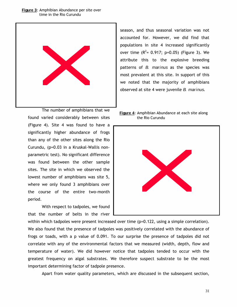
UFigure 3

season, and thus seasonal variation was not

accounted for. However, we did find that

populations in site 4 increased significantly

over time (R2= 0.917; p=0.05) (Figure 3). We

attribute this to the explosive breeding

patterns of B. marinus as the species was

most prevalent at this site. In support of this

we noted that the majority of amphibians

observed at site 4 were juvenile B. marinus.

The number of amphibians that we

found varied considerably between sites

(Figure 4). Site 4 was found to have a

significantly higher abundance of frogs

than any of the other sites along the Rio

Curundu, (p=0.03 in a Kruskal-Wallis non-

parametric test). No significant difference

was found between the other sample

sites. The site in which we observed the

lowest number of amphibians was site 5,

where we only found 3 amphibians over

the course of the entire two-month

period.

With respect to tadpoles, we found

that the number of belts in the river

within which tadpoles were present increased over time (p=0.122, using a simple correlation).

We also found that the presence of tadpoles was positively correlated with the abundance of

frogs or toads, with a p value of 0.091. To our surprise the presence of tadpoles did not

correlate with any of the environmental factors that we measured (width, depth, flow and

temperature of water). We did however notice that tadpoles tended to occur with the

greatest frequency on algal substrates. We therefore suspect substrate to be the most

important determining factor of tadpole presence.

Apart from water quality parameters, which are discussed in the subsequent section,

U: Amphibian Abundance per site over time in the Rio Curundu

Figure 4: Amphibian Abundance at each site along the Rio Curundu

31

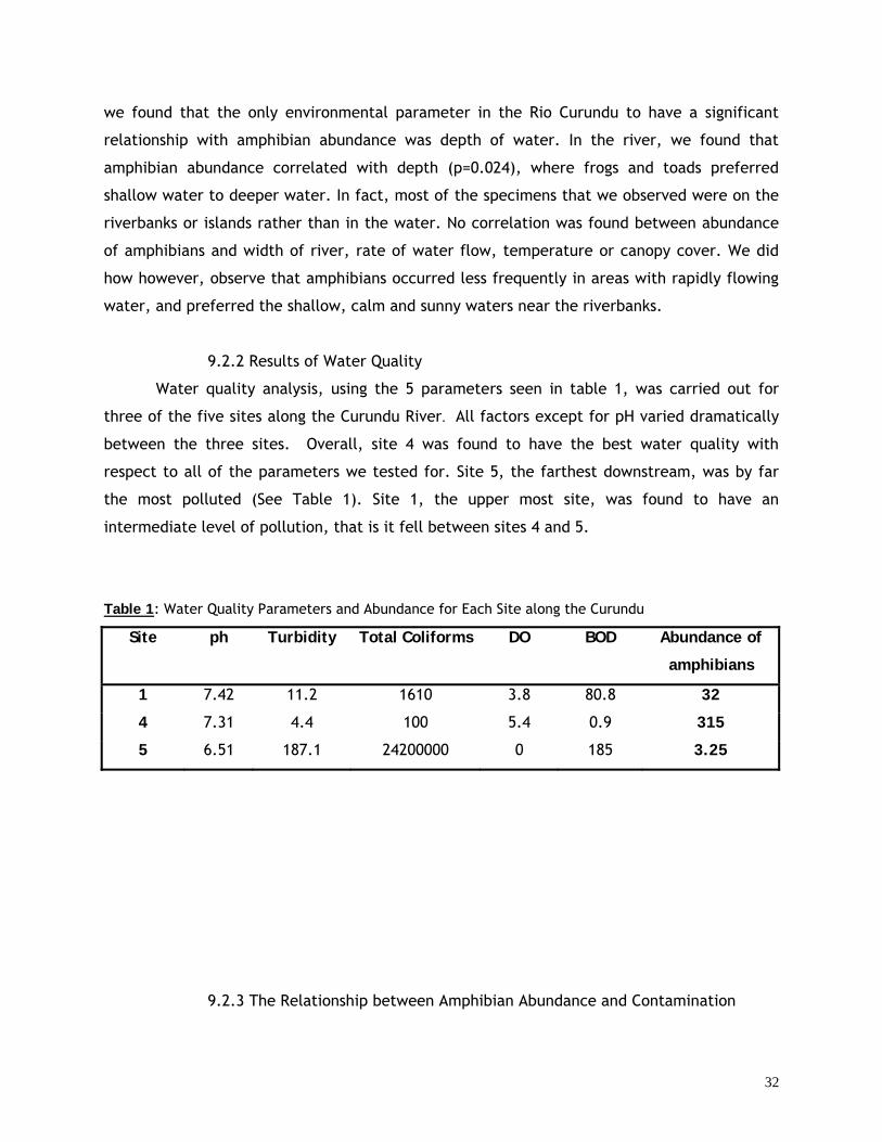
we found that the only environmental parameter in the Rio Curundu to have a significant

relationship with amphibian abundance was depth of water. In the river, we found that

amphibian abundance correlated with depth (p=0.024), where frogs and toads preferred

shallow water to deeper water. In fact, most of the specimens that we observed were on the

riverbanks or islands rather than in the water. No correlation was found between abundance

of amphibians and width of river, rate of water flow, temperature or canopy cover. We did

how however, observe that amphibians occurred less frequently in areas with rapidly flowing

water, and preferred the shallow, calm and sunny waters near the riverbanks.

9.2.2 Results of Water Quality

Water quality analysis, using the 5 parameters seen in table 1, was carried out for

three of the five sites along the Curundu River. All factors except for pH varied dramatically

between the three sites. Overall, site 4 was found to have the best water quality with

respect to all of the parameters we tested for. Site 5, the farthest downstream, was by far

the most polluted (See Table 1). Site 1, the upper most site, was found to have an

intermediate level of pollution, that is it fell between sites 4 and 5.

Table 1: Water Quality Parameters and Abundance for Each Site along the Curundu

Site ph Turbidity Total Coliforms DO BOD Abundance of

amphibians

1 7.42 11.2 1610 3.8 80.8 32

4 7.31 4.4 100 5.4 0.9 315

5 6.51 187.1 24200000 0 185 3.25

9.2.3 The Relationship between Amphibian Abundance and Contamination

32

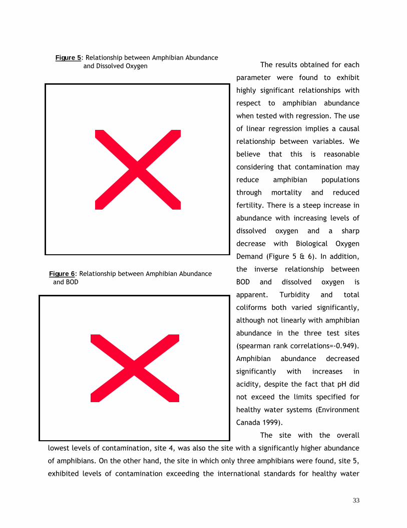
Figure 5: Relationship between Amphibian Abundance

and Dissolved Oxygen The results obtained for each

parameter were found to exhibit

highly significant relationships with

respect to amphibian abundance

when tested with regression. The use

of linear regression implies a causal

relationship between variables. We

believe that this is reasonable

considering that contamination may

reduce amphibian populations

through mortality and reduced

fertility. There is a steep increase in

abundance with increasing levels of

dissolved oxygen and a sharp

decrease with Biological Oxygen

Demand (Figure 5 & 6). In addition,

the inverse relationship between

BOD and dissolved oxygen is

apparent. Turbidity and total

coliforms both varied significantly,

although not linearly with amphibian

abundance in the three test sites

(spearman rank correlations=-0.949).

Amphibian abundance decreased

significantly with increases in

acidity, despite the fact that pH did

not exceed the limits specified for

healthy water systems (Environment

Canada 1999).

The site with the overall

lowest levels of contamination, site 4, was also the site with a significantly higher abundance

of amphibians. On the other hand, the site in which only three amphibians were found, site 5,

exhibited levels of contamination exceeding the international standards for healthy water

Figure 6: Relationship between Amphibian Abundance and BOD

33

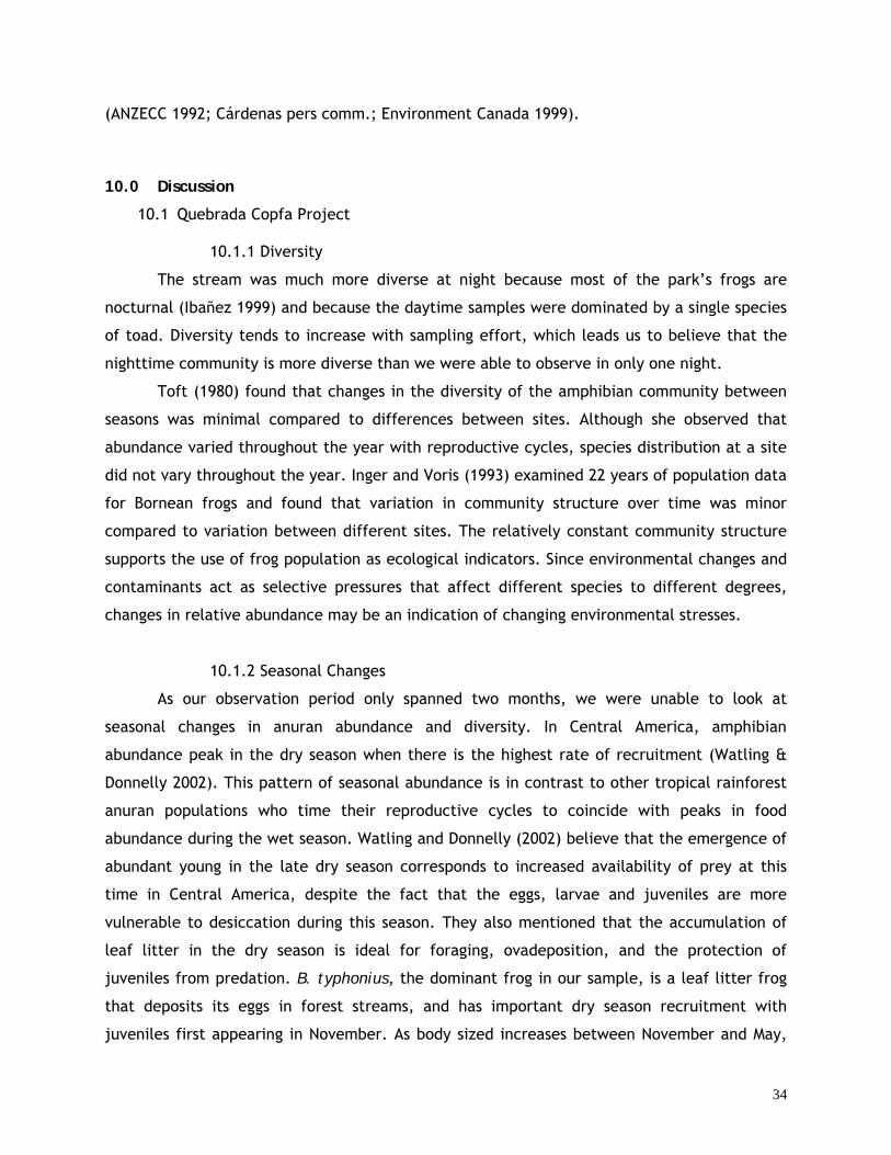
(ANZECC 1992; Cárdenas pers comm.; Environment Canada 1999).

10.0 Discussion

10.1 Quebrada Copfa Project

10.1.1 Diversity

The stream was much more diverse at night because most of the park’s frogs are

nocturnal (Ibañez 1999) and because the daytime samples were dominated by a single species

of toad. Diversity tends to increase with sampling effort, which leads us to believe that the

nighttime community is more diverse than we were able to observe in only one night.

Toft (1980) found that changes in the diversity of the amphibian community between

seasons was minimal compared to differences between sites. Although she observed that

abundance varied throughout the year with reproductive cycles, species distribution at a site

did not vary throughout the year. Inger and Voris (1993) examined 22 years of population data

for Bornean frogs and found that variation in community structure over time was minor

compared to variation between different sites. The relatively constant community structure

supports the use of frog population as ecological indicators. Since environmental changes and

contaminants act as selective pressures that affect different species to different degrees,

changes in relative abundance may be an indication of changing environmental stresses.

10.1.2 Seasonal Changes

As our observation period only spanned two months, we were unable to look at

seasonal changes in anuran abundance and diversity. In Central America, amphibian

abundance peak in the dry season when there is the highest rate of recruitment (Watling &

Donnelly 2002). This pattern of seasonal abundance is in contrast to other tropical rainforest

anuran populations who time their reproductive cycles to coincide with peaks in food

abundance during the wet season. Watling and Donnelly (2002) believe that the emergence of

abundant young in the late dry season corresponds to increased availability of prey at this

time in Central America, despite the fact that the eggs, larvae and juveniles are more

vulnerable to desiccation during this season. They also mentioned that the accumulation of

leaf litter in the dry season is ideal for foraging, ovadeposition, and the protection of

juveniles from predation. B. typhonius, the dominant frog in our sample, is a leaf litter frog

that deposits its eggs in forest streams, and has important dry season recruitment with

juveniles first appearing in November. As body sized increases between November and May,

34

population size decreased, which is explained by increase in mortality and dispersal (Toft,

1982). Although we did not measure body size, we found that the abundance of B. typhonius

decreased significantly between early February and late March.

Toft (1982) noted that frogs bred at irregular periods in the artificial pond on Barro

Colorado Island, which has constant water levels throughout the year. The fact that the

Quebrada Copfa has a cement bottom which affects water levels, it may also influences the

timing of frog recruitment. As most natural streams in the park were dry during the months of

February and March, the artificial segment of Quebrada Copfa probably leads to a local

increase in frog population during the dry season. As frogs play diverse ecosystem roles,

including predators to litter arthropods and prey to various snakes, birds and mammals, the

ecological impacts of amphibians on this stream may be quite substantial.

10.1.3 Environmental Factors

Because amphibians are ectothermic animals and therefore cannot internally regulate

their body temperature, water temperature is an important determining factor in amphibian

micro-habitat selection. Furthermore, because amphibians are poikilotermic, temperature

has an effect on several biological processes such as water balance, digestion, oxygen uptake,

vision, hearing, emergence from hibernation, calling, development, metamorphosis, growth,

regeneration, mitosis, sex reversal, and immune response (Rome et al.1992, in Donnelly &

Crump 1998). Moreover, correlations between ambient temperature and behaviour seem to

suggest that daily and seasonal activity patterns may be affected by temperature (Rome et al.

1992, in Donnelly & Crump 1998).

Water temperature tended to increase over the two months we monitored the

quebrada, corresponding with lower water levels and correlating with an overall decrease in

frog populations. It is possible that the variation in temperature was not great enough to

affect habitat selection in our study. In this case, temperature and amphibian abundance are

not causally linked but affected simultaneously by seasonal changes. However, as previously

discussed temperature does have important implications on amphibian survivorship.

Leaf litter was positively correlated with toad abundance in the stream, despite the

fact that it tends to accumulate in mass quantities towards the end of the dry season. Toft

(1980) also found that leaf litter was weakly correlated with the abundance of B. typhonius

juveniles, and hypothesized that the leaf litter provided cover from predators.

Jaeger & Hailman (1981) studied light as an environmental factor in niche selection.

They found that light gradients affected habitat partitioning in three ways including:

35

photoactic behavior, microhabitat habitat selection, and daily activity periods, allowing

species to co-exist sympatrically. Factors like time of day, forest cover, and leaf litter would

affect the light, and thus are potentially important determinants of amphibian abundance and

species diversity. We found no relationship between the percentage of foliage cover and

amphibian abundance in the belts. However, our diversity study does show that there is an

important difference in the community structure depending on time of day.

None of the environmental factors we measured were significant enough to account

for the differences in frog abundance between the three sites. This may be a result of the

lack of precision in our method of quantifying some variables. It may also be due to

environmental factors that we were unable to quantify such as abundance of prey, levels of

contamination, or proximity to breeding sites.

The paved quebrada has very limited variation with respect to environmental factors. This

may explain why factors such as stream width and depth are insignificant in this study despite

being the most important determinants of amphibian distribution in other studies (Inger &

Voris 1993). The most important environmental determinant we observed was the presence or

absence of water, as is apparent from the plummeting population in site 9 when the quebrada

dried up in mid-March (Figure 2).

10.2 Curundu Project

10.2.1 Environmental Factors

Our results show that considerable differences exist between sites for both amphibian

abundance and degree of water contamination. Results form the Rio Curundu suggest that the

most important determinants of amphibian abundance within the Rio are the water quality

parameters. Our analysis indicates that the environmental parameters, such as water depth,

which under natural conditions affect amphibian abundance, are overridden by the more

powerful determinants of water quality. That is to say, if the water is uninhabitable for

amphibians then the suitability of habitat (i.e. water depth and flow, canopy coverage, etc.)

become irrelevant. However, when contamination is minimal, these environmental factors

are the determining factor.

The strength of the correlations between amphibian abundance and water quality

demonstrates that amphibians are extremely sensitive to environmental conditions, thus

supporting the notion that they make good indicators of environmental health (Roy 2002;

Welsh and Ollivier 1998).

36

10.2.2 Water Quality

The differences in water quality that we found between the three sites were quite

dramatic and the results that were obtained from the water analysis were surprising. Our

initial hypothesis was that the abundance of amphibians would be greatest at the most

upstream site (site 1), which we believed would be the site with the cleanest water, and

decrease as the sites continued downstream and the water became more and more polluted.

This rested on the assumption that water quality decreased as contaminants accumulated

towards the bottom of the river. This assumption was based on the information we had

received from both the director of PNM, Felix Wing-Solís, and from our park guide, Sixto

Mequizama, who has been with the park for over 10 years and who is extremely

knowledgeable regarding the state of the environment in PNM. We were informed that the

water would be cleanest at the most upstream site and would get progressively more polluted

as the river travels downstream.

However, our results undermined this assumption. In fact, the site with the cleanest

water was site 4, immediately upstream from the site with the most polluted water, site 5. In

addition, site 1, which we had expected would have the cleanest water and the greatest

abundance of amphibians, exhibited an intermediary level of both.

The reasons for the varying levels of contamination along the Rio Curundu are

unknown to us. There is a remarkable difference in visible water quality between sites 4 and

5. Our guide, Sixto Mequizama, as well as Professor Cenobio Cárdenas from the Universidad

Tecnologica de Panamá, stated that the grey-white pulpy material that is found in site 5 and

is absent from all other sites is in fact a mixture of paper pulp and the by-products of the

beer factory. This leads us to believe that one of the major and most important differences

between sites 5 and 4 is a point source of pollution dumping organic wastes and other

contaminants from these two industries into the river downstream from site 4 and just

upstream from site 5. In addition, we have been informed that just above site 5 there is a

pipe that dumps vast amounts of raw, untreated sewage from the impoverished

neighbourhood of Curundú into the river (Mequizama, pers. comm.).

The grey paper pulp would explain the extremely high level of turbidity (more than 16

times the level of turbidity found at either of the other two sites analysed) found at this site

5. In addition, the dumping of organic by-products of beer production as well as untreated

sewage into the Curundu just upstream from site 5 could explain the exceptionally high levels

of BOD (185 mg/L). More information would be needed to determine whether these two

sources of organic waste are the only two contributors to the poor water quality. BOD levels

37

in site 5 were more than twice as high as they were in site 1 and over 200 times as high as

they were in site 4 (which, as mentioned, is ironically the upstream site adjacent to site 5).

The elevated levels of BOD that were encountered at site 5 could explain the

complete absence of dissolved oxygen in the water at this site. The overabundance of organic

waste materials in the water means that there is also an overabundance of bacterial micro-

organisms in the water that are using dissolved oxygen to assimilate the organic waste. The

lack of dissolved oxygen in the water analysis for this site means that oxygen is being

consumed as quickly as it is being produced and replenished in the water (Blaustein et al.

2003). The presence of industrial waste could also explain the relatively lower pH, 6.51 that

was found in site 5 as compared to the other sites (where pH was above 7). The total coliform

count, which measured 24,000,000 coliforms per 100mL of water, with equally high levels of

E. coli, are explained by the presence of the sewage pipe carrying untreated sewage into the

river.

Cenobio Cárdenas, of the Universidad Tecnologica de Panama, hypothesised that one

factor that could explain the higher levels of dissolved oxygen at site 4 as compared with site

5 and site 1 is that the water in and upstream of site 4 runs fairly rapidly over rocks and

bumps, allowing for oxygen to be taken up, thus increasing the levels of dissolved oxygen in

the site. In both site 1 and site 5, the water movement and the amount of turbulence were

lower, meaning that not as much oxygen is mixed into the water. Another factor contributing

to high levels of dissolved oxygen in site 4 could be that the levels of BOD were low in this

site at only 0.9 mg/L, meaning that the dissolved oxygen in the water at this site was not

being rapidly used. Reasons for the relatively lower level of water quality in site 1, in

comparison to site 4, may be related to the fact that a commercial area, including a car

wash, and a residential area are located near by, in addition to the presence of a major

roadway (Avenida de la Amistad). These factors could lead to increased levels of turbidity and

BOD at site 1, whereas site 4 is far from any industries and major roads.

10.2.3 The Relationship between Amphibian Abundance and Contamination

It is impossible to untangle the magnitude of importance of each factor with relation

to the abundance of amphibians based on our study alone. However, the literature gives us

some clues as to how various contaminants interact with anuran physiology. Amphibian

abundance decreased sharply and significantly with decreasing water quality. In site 5, where

measures of BOD, DO, and coliforms were orders of magnitude above the recommended

levels, we found only three amphibians during the entire study. Furthermore, these were

38

adult specimens found in the leaf litter on the riverbank. The juveniles that made up the

large part of our samples at other sites were not present at site 5, indicating that this part of

the river cannot support amphibian reproduction.

There are many reasons to justify a relationship between water quality and amphibian

abundance. Turbidity and sedimentation have been shown to be significant contributors to

declines in populations of aquatic organisms, including amphibians (Welsh & Ollivier 1998).

High levels of turbidity can limit the penetration of light into the water thereby negatively

affecting photosynthesis capabilities of aquatic vegetation, phytoplankton, and algae.

Sedimentation also has an abrasive quality, scratching and often reducing the quantity of

plant growth in the streambed (Henley et al. 2000). This reduction in plant and algae growth

has effects on higher trophic levels such as the insects that depend on this vegetation for food

(Henley et al. 2000). Furthermore, amphibians in their larval stage depend on algae in the

water for food and habitat, and many adult amphibians depend on insects as their main

source of food (Henley et al. 2000). As turbidity affects both of these resources, the impacts

on the amphibian population will be severe.

Another damaging consequence of turbidity and suspended sediment is the direct

hazard they pose for gilled organisms as fine sediments can clog the gills of fish and tadpoles

(Ibañez, pers. comm.). In addition, particles of silt and clay that settle to the bottom can

suffocate newly hatched fish and amphibian larvae (Welsh & Ollivier 1998; Ibañez, pers.

comm.). Furthermore, because suspended solids darken the water and absorb more heat from

the sun, turbid water usually becomes warmer and can become unsuitable for amphibians

(Duellman & Trueb 1986). Increases in both turbidity and temperature are paralleled by

decreases in the amount of dissolved oxygen in the water (Duluth Streams 2003).

We found there to be no dissolved oxygen at site 5. This may be the result of high

levels of turbidity, as well as organic wastes and sewage in the waterway. When high levels of

organic wastes and sewage are present, the associated micro-organisms, such as coliforms,

consume dissolved oxygen in the decomposition of these wastes, out competing amphibians

for the ever shrinking oxygen supply. This competition for dissolved oxygen is confirmed by

the intolerably high level of both BOD and total coliforms found at site 5. Furthermore, Rouse

et al. (1999) noted that nitrogen in the water, introduced by faecal coliforms, can have

harmful effects on amphibian larva such as reductions in feeding activities, reduced vigour,

development of malformations of the body, and even death.

Although we have seen that acidity negatively affects amphibians, pH varied between

the three sites by less than one, which would not usually have a significant impact on

39

amphibian populations (Environment Canada 1999). However, because the most acidic site

was also polluted in other more important ways, this relationship appears to be significant

within the context of the Curundu. Furthermore, in laboratory studies, the toad Bufo

marinus, did not exhibit significant negative effects when exposed to acidic water for 2 weeks

(Simon et al. 2002), indicating that it is probably one amphibians most resistant to acidity.

Although our initial assumption about the distribution of contaminants in the Curundu

River was false, the data does show that pollution is the most important limiting factor on

amphibian populations in the river. All the water quality parameters we tested for were

significantly correlated with amphibian abundance, which supports our hypothesis that

amphibian abundance is inversely related to water quality. As the water quality deteriorates

the abundance of amphibians will decrease.

11.0 Conclusion and Recommendations

Our first goal was to establish a protocol by which we could assess whether amphibian

populations are declining in Parque Natural Metropolitano. This particular objective would

necessitate monitoring amphibian populations for several years. As the park has limited

resources to dedicate to monitoring amphibians, we recommended that they use high-school

students as volunteers in an on-going monitoring program of amphibians that would take off

from our baseline collection of data. Although the park promotes its educational facilities,

and does have a relationship with local schools, this is the first effort, as far as we know, to

involve high school students in a scientific study. Involving high school students in this project

is mutually beneficial to both the park and the youths. The exercise will educate youths about

local wildlife and the threats to biodiversity throughout the globe, in addition to giving

students a chance to experience nature, to work in the field, and become involved with a

local NGO. PNM will benefit from the information gathered by the students, as well as

developing or strengthening ties with the community.

To get this project underway, we have devised a simple methodology to sample frogs

in the Quebrada Copfa, in addition to providing baseline data for diurnal amphibian

abundance for the months of February and March. We have also created educational material

about the biology and ecological importance of amphibians, as well as their potential as

ecological indicators.

We found that the anuran community varied significantly between day and night, and

that diversity of nocturnal species was much higher. Our project was limited to monitoring

diurnal species, primarily the toad Bufo Typhonius. A more complete monitoring including

40

nocturnal frogs is needed to properly assess amphibian populations as a whole. Furthermore,

a similar monitoring effort is required during the wet season in order to properly census all

amphibian species and their respective population trends.

In collecting baseline data for the monitoring project, we were able to analyse how

amphibians interact with their environments. We found that seasonal change was the factor

with the strongest influence on amphibian abundance. Seasonal change included the presence

or absence of water, which was found to be a key predictor of amphibian distribution in the

Quebrada Copfa. Temperature and amount of leaf litter are other factors we found to be

significant, however the relationship was not as strong. Our experience with sampling in the

Quebrada Copfa highlighted the importance of considering natural fluctuations and micro-

environmental factors when looking at the effects of anthropogenic factors on amphibians.

Our second goal was to examine the effects of pollutants on amphibian populations in

the Curundu River. We found that the abundance of amphibians peaked in site 4, towards the

bottom or the river, and did not decrease from north to south as we had predicted. These

surprising results prompted us to look more in depth at several water quality parameters. We

found that water quality was the highest at site 4, corresponding with the highest abundance

of toads. This was in contrast with our assumption that water quality progressively

deteriorated as the river flowed from north to south. Despite our initial assumption being

false, our data strongly supported the hypothesis that amphibian abundance decreases with

pollution. We suspect that environmental factors such as substrate, surrounding vegetation,

and gradient of the river also affect amphibian distribution in the river, but unfortunately, we

were unable to quantify these variables in our study.

The results of our study on contamination support the use of amphibians as indicators

of ecological health in forest streams. This justifies the need to continue monitoring

amphibians in order to determine the overall population trend in PNM. Unfortunately, many

of the anthropogenic stresses on the amphibian population are beyond the control of the

park. The quality of the water in the Curundu River, and thus the state of the amphibians in

the river, are products of the political context in which the park is found. PNM was created by

a law in 1988, and over the past ten years there has been no environmental legislation in

Panama protecting the waterways of the park from industrial pollution. In 1998, the

government of Panama did however, pass the first environmental law of Panama. This law

made the dumping of untreated industrial waste illegal, and necessitated the cleaning and

filtering of organic and industrial wastes before they were released into the environment

(Felix Wing-Solís, pers. comm.). As our results have shown, this will have important

41

implications for the state of water quality in the Curundu river, as the situation can only get

better in site 5. However, the law did not go into effect until 2001, at which point the

legislation has given industry a 9-year grace period in order to counter the shock and ease the

transition into the new regulations. This means that for the 9 year period between 2001 and

2010, industries will be legally allowed to continue their release of untreated wastes into

waterways such as the Curundu River. It is impossible to say whether this will deteriorate the

ecosystem that depends on the water of the river even further, or how long it will take the

water of this river, especially in the most polluted sites, to improve. Therefore, it is our

hope that the information provided in this report on the effects of pollution on local anuran

populations will support the park in calling for environmental regulation of contaminants to

be more speedily and rigorously enforced.

42

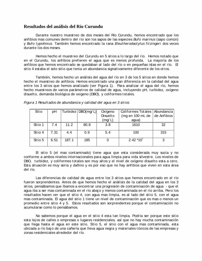
Resultados del análisis del Río Curundu

Durante nuestro muestreo de dos meses del Río Curundu, hemos encontrado que los anfibios mas comunes dentro del río son los sapos de las especies Bufo marinus (sapo común) y Bufo typohnius. También hemos encontrado la rana Eleutherodactylus fitzingeri dos veces durante los dos meses.

Hemos hecho el muestreo del Curundu en 5 sitios a lo largo del río. Hemos notado que

en el Curundu, los anfibios prefieren el agua que es menos profunda. La mayoría de los anfibios que hemos encontrado se quedaban al lado del río o en pequeñas islas en el río. El sitio 4 estaba el solo sitio que tenia un abundancia signativamente diferente de los otros.

También, hemos hecho un análisis del agua del río en 3 de los 5 sitios en donde hemos

hecho el muestreo de anfibios. Hemos encontrado una gran diferencia en la calidad del agua entre los 3 sitios que hemos analizado (ver Figura 1). Para analizar el agua del río, hemos hecho muestreos de varios parámetros de calidad de agua, incluyendo pH, turbidez, oxígeno disuelto, demanda biológica de oxigeno (DBO), y coliformes totales. Figura 1 Resultados de abundancia y calidad del agua en 3 sitios

Sitio pH Turbidez DBO(mg/L) Oxígeno Disuelto (mg/L)

Coliformes Totales (mg en 100 mL de

agua)

Abundancia de Anfibios

Sitio 1 7.4 11.2 80.8 3.8 1610 32

Sitio 4 7.31 4.4 0.9 5.4 100 315

Sitio 5 6.51 187.1 185 0 2.42 *107 3

El sitio 5 (el mas contaminado) tiene agua que esta considerada muy sucia y no

conforme a ambos niveles internacionales para agua limpia para vida silvestre. Los niveles de DBO, turbidez, y coliformes totales son muy altos y el nivel de oxígeno disuelto esta a cero. Esta situación es muy seria y dañino y es por eso que no hay anfibios que viven en esta área del río.

Las diferencias de calidad de agua entre los 3 sitios que hemos encontrado en el río

fueron sorprendentes. Antes de que hemos hecho el análisis de la calidad del agua en los 3 sitios, pensábamos que íbamos a encontrar una progresión de contaminación de agua - que el agua iba a ser mas contaminada en el río abajo y menos contaminada en el río arriba. Pero los resultados hacen ver que el sitio 4, con agua mas limpia, es al lado del sitio 5, con el agua mas contaminada. El agua del sitio 1 tiene un nivel de contaminación que es mas o menos un promedio entre sitio 4 y 5. Estos resultados son sorprendentes porque el contaminación no acumularse como lo pensábamos.

No sabemos porque el agua en el sitio 4 esta tan limpia. Podría ser porque este sitio

esta lejos de calles o empresas o lugares residenciales, así que no hay mucha contaminación que llega hasta el agua en este sitio. Sitio 5, el sitio con el agua mas contaminada, esta ubicada a río bajo de una cañería que lleva agua negra y materiales tóxicos de las empresas y zonas residenciales alrededor del río.

Pueden ver en los resultados de la Figura 1 que la abundancia de los anfibios depende mucho de la calidad del agua en donde viven. Todos los parámetros tenían relaciones significativas con la abundancia. Pero pensamos que los factores más importantes son la turbidez y el cantidad de oxigeno disuelto en el agua.

La turbidez es una medida de las partículas en el agua. Esas partículas pueden atascar

las branquias de los renacuajos. Demás, cuando hay mucho turbidez, hay menos luz para las plantas acuáticas. Los renacuajos comen y viven en las plantas acuáticas. Los insectos, que forman una parte importante de la alimentación de las ranas adultas, se alimentan también des las plantas acuáticas. Entonces, una alta turbidez es dañina para las poblaciones de ranas por varias razones.

En el sitio 5, no había ningún oxigeno disuelto, y entonces la vida acuática no se puede sostener. La DBO estaba muy alta. Eso confirme que el oxigeno esta usado por las bacterias para descomponer aguas negras y otros productos contaminantes.

En el sitio 4, todos los parámetros de contaminación parecen normales, y hay una

población sana de sapos de la especie Bufo marinus.

12.0 Works Cited

ANZECC. Australian and New Zealand Water Quality Guidelines. 1992. www.mfe.govt.nz. Ministry for the Environment, New Zealand. Asemblea Legeslativa. 1985. Decreto, Ley No. 8. Por la cual se crea el Parque Natural Metropolitano. Asemblea Legeslativa. 1967. Decreto, ley No. 23. Protección y Conservación de la Fauna Silvestre. Beattie, Robert & Richard Tyler-Jones. 1992. The Effects of Low pH and Aluminium on Breeding Success in the Frog Rana temporaria. Journal of Herpetology 26 (4): 353-360. Berven, K. A. 1990. Factors affecting population fluctuations in larval and adult stages of the wood frog (Rana sylvatica). Ecology 71: 1599-1608. Biek, Roman, Chris Funk, Bryce Maxell, & Scott Mills. 2002. What is Missing in Amphibian Decline Research: Insights from Ecological Sensitivity Analysis. Conservation Biology 16(3): 728-734. Blaustein, A. R., Romansic, J.M., Kiesecker, J.M., & Audrey Hatch. 2003. Ultraviolet Radiation, Toxic Chemicals and Amphibian Population Declines. Diversity and Distributions 8(2): 123-136 Blaustein, Andrew R. 1994a. Chicken little or Nero’s fiddle? A perspective on declining amphibian populations. Herpetologica 50(1): 85-97. Blaustein, Andrew R. et al. 1994b. UV repair and resistance to solar UV-B in amphibian eggs: a link to population declines? Proceedings of the National Academy of Science, USA 91: 1791-1795. Bradford, David & Malcolm S. Gordon. 1995. Aquatic Amphibians in the Sierra Nevada: Current Status and Potential Effects of Acidic Deposition on Populations. California Environmental Protection Agency. www.arb.ca.gov Bradford, D.F., Christina Swanson & Malcolm S. Gordon. 1992. Effects of Low pH and Aluminium on Two Declining Species of Amphibians in the Sierra Nevada, California. Journal of Herpetology 26(4): 369-377. Brandt, Laura A. & Frank J. Mozzotti. 2003. Marine Toads (Bufo Marinus). University of Florida. http://edis.ifas.ufl.edu Carey, Cynthia & Michael A. Alexander. 2003. Climate change and amphibian declines: Is there a link? Diversity and Distributions 9(2): 111-123. Carey, Cynthia. 1993 Hypothesis concerning the disappearance of Boreal Toads from the mountains of Colorado. Conservation Biology 7: 355-362.

43

Cárdenas, Cenubio. 2003. Professor of water chemistry at the Instituto Tecnologica de Panama. Chen B. & D. Wise. 1999. Bottom-Up Limitation of Predaceous Arthropods in a Detritus-Based Terrestrial Food Web. Ecology 80(3): 761-772. Collins, James P. & Andrew Storfer. 2003. Global amphibian declines: Sorting the hypotheses. Diversity and Distributions 9(2): 89-99. Corn, Paul S. & Frank A. Vertucci. 1992. Descriptive Risk Assessment of the Effects of Acidic Deposition on Rocky Mountain Amphibians. Journal of Herpetology 26(4): 361-369. Donnelly, Maureen A. & Martha L. Crump. 1998. Potential Effects of Climate Change on Two Neotropical Amphibian Assemblages. Climatic Change 39: 541-561. Duellman, William E. & Linda Trueb. 1986. Biology of Amphibians. Baltimore, USA: The John Hopkins University Press. Duluth Streams. 2003. www.duluthstreams.org Colegio de la Fontera Sur (ECOSUR), Smithsonian Tropical Research Institute (STRI), & Pontificia Universidad Catolica del Ecuador (PUCE). 1999. Disminución de la población anfibia en América Latina: Informe acerca de los tres Talleres internacionales realizados para evaluar el problema y priorizar necesidades. Drost, C.A. & G.M. Fellers. 1996. Collapse of a regional frog fauna in the yosemite area of the California Sierra Nevada, USA. Conservation Biology 10: 414-425. Dunson, W.A et al. 1992. A symposium on amphibian declines and habitat acidification. Journal of Herpetology 26: 349-352. Environment Canada. 1998. www.ec.gc.ca/water/en/manage/qual/e_qual.htm Fetcher, N. et al. 1985. Vegetation effects on microclimate in lowland tropical forests in Costa Rica. International Journal of Biometerol 29: 145-155. Green, David. 2003. Herpotalogist, McGill University. Personal Comment. Henley, W.E., M.A. Patterson, R.J. Neeves & Dennis Lemly. 2000. Effects of Sedimentation and Trubidity on Lotic Food Webs: A Concise Review for Natural Resource Managers. Reviews in Fisheries Science 8(21): 125-139. Houlahan, J. E. et al. 2000. Quantitative evidence for global amphibian population declines. Nature 404: 752-755. Ibañez, Roberto. 2003. Herpetologist, Smithsonian Tropical Research Institute. Personal comment.

44

Ibañez, Roberto D. et al. 1999. Los Anfibios del Monumento Natural Barro Colorado Parque Natural Soberania y Areas Adyacentes. Smithsonian Tropical Research Institute: Colombia. P 187. Inger, R F & Voris, H K. 1993. A comparison of amphibian communities through time and from place to place in bornean forests. Journal of Tropical Ecology 9: 409-433. Jaeger, R G & Hailman, J P. 1981. Activity of neotropical frogs in relation to ambient light. Biotropica 13(1): 59-65. Jaeger, R.G. 1980. Density dependent and density independent causes of extinction of a salamander population. Evolution (24): 632-634. Kerr, J.B & C. T. McElroy. 1993. Evidence for Large Upward Trends of Ultraviolet-B Radiation Linked to Ozone Depletion. Science 262 (5136): 1032-1034. Kiesecker, Joseph M. et al. 2001. Complex causes of amphibian population declines. Nature 410: 681-683. Lips, Karen R. 1999. Mass Mortality and Population Declines of Anurans at an Upland Site in Western Panama. Conservation Biology 13(1): 117-125. Lips, Karen R. 1998. Decline of a Tropical Montane Amphibian Fauna. Conservation Biology 12(1): 106-117. Mattison, Chris. 1987. Frogs and Toads of the World. Blandford Press: New York. Mequizama, Sixto. 2003. Park guide at Parque Natural Metropolitano, Panama. Personal comment. Parque Natural Metropolitano (PNM). 2002. “Organizacion”. www.parquenp.org Parque Natural Metropolitano (PNM). 1999a. Plan de Manejo del Parque Natural Metropolitano Parque Natural Metropolitano (PNM). 1999b. Plan de Manejo del Parque Natural Metropolitano – Resumen Ejecutivo. Fundacion Natura, Panama. p 28. Parque Natural Metropolitano (PNM). 1998. Memorias Parque Natural Metropolitano: Trece Años de Conservación. PMCC. Proyecto de Monitoreo Ecologico de la Cuenca del Canal de Panama. www.stri.org/PMCC Rouse, J. et al. 1999. Nitrogen Pollution: An Assessment of its Threats to Amphibian Survival. Environmental Health Perspectives 107(10): 799-803. Roy, Debjani. 2002. Amphibians as environmental sentinels. Journal of Bioscience 27 (3): 187-188. Sadinski, W.J & William A. Dunson. A Multilevel Study of Effects of Low pH on Amphibians of Temporary Ponds. Journal of Herpetology 26(4): 413-422.

45

Seebacher, Frank & Ross A. Alford. 2002. Shelter Microhabitats Determine Body Temperature and Dehydration Rates of a Terrestrial Amphibian (Bufo Marinus). Journal of Herpetology 36(1): 69-75. Simon, M.P. et al. 2002. Effects of Acid Exposure on Natural Resistance and Mortality of Adult Rana pipiens. Journal of Herpetology 36(4): 697-699. Stream Watch. 2003. www.streamwatch.org Toft, C A. 1982. Population Dynamics and seasonal recruitment in Bufo typhonius and Colostethus nubicola (Anura). Leigh, E G. Rand, A S. and Windsor D M. (eds). In The ecology of a tropical forest: 397-403. Washington, DC: Smithsonian Institution Press. Toft, C A. 1980. Seasonal variation in populations of Panamanian leaf litter frogs and their prey: a comparison of wetter and drier sites. Oecologia 47: 34-38 University of Michigan. 2003. http://animaldiversity.ummz.umich.edu Vredenburg, Vance T. 1998. Introduced predators, amphibian declines, and the use of chemical cues in predator recognition: does history matter? International Society of Behavioural Ecology Meeting. http://ist-socrates.berkeley.edu/~vancev/ISBE1998.htm Wake, D.B. 1991. Declining amphibian populations. Science 253: 860-867. Warkentin, Karen. 2000. Environmental and Developmental Effects on External Gill Loss in the Red-Eyed Tree Frog, Agalychnis callidryas. Physiological and Biochemical Zoology 73(5): 557-565. Watling, J I. & Donnelly, M A. 2002. Season patterns of reproduction and abundance of leaf litter frogs in a Central American rainforest. Journal of Zoology. London. 258: 269-276. Welsh, Hartwell H., & Lisa M. Ollivier. 1998. Stream amphibians as indicators of ecosystem stress: A case study from California’s Redwoods. Ecological Applications 8(4): 1118-1132. Welsh, Hartwell H., & Garth R. Hodgson. 1997. A hierarchical strategy for sampling herpetofaunal assemblages along small streams in the western U.S. with an example from northern California. Transactions of the western section of the wildlife society 33: 56-66. Welsh, Hartwell H., Amy J. Lind, & Dana L. Waters. 1991. Monitoring Frogs and Toads in Region 5 National Forests. Fish Habitat Relationship Technical Bulletin, Number 4. Young, Bruce E. et al. 2001. Population Declines and Priorities for Amphibian Conservation in Latin America. Conservation Biology 15(5): 1213-1223.

46