regresion por minimos cuadrados

i x y xy x2 (y-y^)2 (y-y-)21 1 1 1 1 2.41975309 18.29938272 2 1.5 3 4 0.35667438 14.27160493 3 2 6 9 0.13040123 10.74382724 4 3 12 16 0.6714892 5.18827165 5 4 20 25 1.63271605 1.632716056 6 5 30 36 3.01408179 0.077160497 7 8 56 49 0.03780864 7.410493838 8 10 80 64 0.12056327 22.29938279 9 13 117 81 3.56790123 59.632716

SUM 45 47.5 325 285 11.9513889 139.555556

A0 1.458333333A1 -2.013888889 Y media 5.277777778X media 5

Y estimada 1.458333333 -2.013888889 x

St 139.55555Sr 11.95138889Sy/x 1.306652697R2 0.914361067R 0.956222289

0 1 2 3 4 5 6 7 8 9 100

2

4

6

8

10

12

14

Column CLinear (Column C)

0 1 2 3 4 5 6 7 8 9 100

2

4

6

8

10

12

14

Column CLinear (Column C)

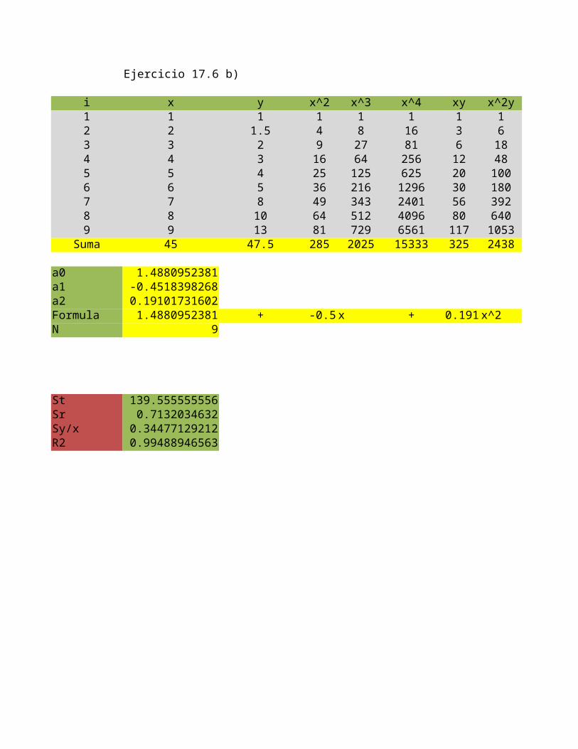
Ejercicio 17.6 b)

i x y x^2 x^3 x^4 xy x^2y (y-y^)21 1 1 1 1 1 1 1 0.0522 2 1.5 4 8 16 3 6 0.0233 3 2 9 27 81 6 18 0.0224 4 3 16 64 256 12 48 0.0695 5 4 25 125 625 20 100 2E-056 6 5 36 216 1296 30 180 0.4277 7 8 49 343 2401 56 392 0.0998 8 10 64 512 4096 80 640 0.019 9 13 81 729 6561 117 1053 0.011

Suma 45 47.5 285 2025 15333 325 2438 0.713

a0 1.488095238095a1 -0.45183982684a2 0.191017316017Formula 1.488095238095 + -0.45 x + 0.191 x^2N 9

St 139.5555555556Sr 0.713203463203Sy/x 0.344771292116R2 0.99488946563

Matriz(y-y-)2

18.299382716 a0 a1 a2 b14.271604938 9 45 285 47.510.74382716 45 285 2025 325

5.1882716049 285 2025 15333 24381.63271604940.0771604938 Determinante 1663207.410493827222.29938271659.632716049139.55555556

0 1 2 3 4 5 6 7 8 9 100

2

4

6

8

10

12

14

f(x) = 0.191017316017316 x² − 0.451839826839826 x + 1.48809523809524R² = 0.994889465629911

Column CPolynomial (Column C)

b a1 a2 a0 b47.5 45 285 9 47.5325 285 2025 45 325

2438 2025 15333 285 2438

δa0 247500 δa1 -75150

0 1 2 3 4 5 6 7 8 9 100

2

4

6

8

10

12

14

f(x) = 0.191017316017316 x² − 0.451839826839826 x + 1.48809523809524R² = 0.994889465629911

Column CPolynomial (Column C)

a2 a0 a1 a2285 9 45 47.5

2025 45 285 32515333 285 2025 2438

δa2 31770

SATURACION

i x y 1/x 1/y (1/x*1/y)1 0.75 1.2 1.33333333 0.83333333 1.111111112 2 1.95 0.5 0.51282051 0.256410263 3 2 0.33333333 0.5 0.166666674 4 2.4 0.25 0.41666667 0.104166675 6 2.4 0.16666667 0.41666667 0.069444446 8 2.7 0.125 0.37037037 0.04629637 8.5 2.6 0.11764706 0.38461538 0.04524887

Σ 32.25 15.25 2.82598039 3.43447293 1.79934431

A1 0.36932005734A0 0.341540242Y prom 0.49063899064X prom 0.40371148459Y estimada 0.341540242 + 0.36932006 x

α 2.92791266455

β 1.08133687317

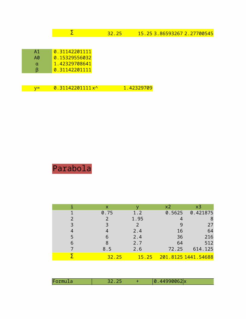
POTENCIA

i x y logx logy log x*log y1 0.75 1.2 -0.12493874 0.07918125 -0.00989282 2 1.95 0.30103 0.29003461 0.087309123 3 2 0.47712125 0.30103 0.143627814 4 2.4 0.60205999 0.38021124 0.228909985 6 2.4 0.77815125 0.38021124 0.295861856 8 2.7 0.90308999 0.43136376 0.38956037 8.5 2.6 0.92941893 0.41497335 0.38568408

Σ 32.25 15.25 3.86593267 2.27700545 1.52106033

A1 0.31142201111A0 0.15329556032α 1.42329708641β 0.31142201111

y= 0.31142201111 x^ 1.42329709

Parabola

i x y x2 x3 x41 0.75 1.2 0.5625 0.421875 0.316406252 2 1.95 4 8 163 3 2 9 27 814 4 2.4 16 64 2565 6 2.4 36 216 12966 8 2.7 64 512 40967 8.5 2.6 72.25 614.125 5220.0625

Σ 32.25 15.25 201.8125 1441.54688 10965.3789

Formula 32.25 + 0.44990062 x +

(1/x)2 Y 1.777777778 1.199088235

0.25 1.9004171140.111111111 2.152171768

0.0625 2.3048364930.027777778 2.480813482

0.015625 2.5792789810.01384083 2.597472355

2.258632497

(log x)2 Y0.015609688 1.301328340.090619058 1.766212390.227644692 2.0039257270.362476233 2.1917463580.605519368 2.4867320270.815571525 2.7198043260.863819539 2.771641601

2.981260104

0 1 2 3 4 5 6 7 8 90

0.5

1

1.5

2

2.5

3

Column DPower (Column D)

0 0.2 0.4 0.6 0.8 1 1.2 1.40

0.1

0.2

0.3

0.4

0.5

0.6

0.7

0.8

0.9

f(x) = 0.369320057343779 x + 0.341540241998453R² = 0.985710791168701

Column FLinear (Column F)

xy0.93.9

69.6

14.421.622.1

78.5

-0.0306938 x^2

0 1 2 3 4 5 6 7 8 90

0.5

1

1.5

2

2.5

3

Column DPower (Column D)

0 1 2 3 4 5 6 7 8 90

0.5

1

1.5

2

2.5

3

Column DPolynomial (Column D)

0 1 2 3 4 5 6 7 8 90

0.5

1

1.5

2

2.5

3

Column DPower (Column D)

0 0.2 0.4 0.6 0.8 1 1.2 1.40

0.1

0.2

0.3

0.4

0.5

0.6

0.7

0.8

0.9

f(x) = 0.369320057343779 x + 0.341540241998453R² = 0.985710791168701

Column FLinear (Column F)

Matriz

a0 a1 a2 b7 32.25 201.8125 15.25

32.25 201.8125 1441.54688 78.5201.8125 1441.54688 10965.3789 511.925

0 1 2 3 4 5 6 7 8 90

0.5

1

1.5

2

2.5

3

Column DPower (Column D)

i x y logx logy logx*logy (log x)21 2.5 13 0.39794001 1.1139433523068 0.44328263 0.158356252 3.5 11 0.54406804 1.0413926851582 0.56658848 0.296010043 5 8.5 0.69897 0.9294189257143 0.64963595 0.488559074 6 8.2 0.77815125 0.9138138523837 0.71108539 0.605519375 7.5 7 0.87506126 0.8450980400143 0.73951256 0.765732216 10 6.2 1 0.7923916894983 0.79239169 17 12.5 5.2 1.09691001 0.7160033436348 0.78539124 1.203211588 15 4.8 1.17609126 0.6812412373756 0.80120186 1.383190659 17.5 4.6 1.24303805 0.6627578316816 0.8238332 1.54514359

10 20 4.3 1.30103 0.6334684555796 0.82416146 1.69267905

Σ 99.5 72.8 9.11125989 8.3295294133471 7.13708446 9.1384018

A1 -0.54028958A0 1.32522482Y prom 0.91112599X prom 0.130103

α 21.145834β -0.54028958

Y= 21.145834 x^ -0.54028958

Y(9)= 6.45145295

0 5 10 15 20 250

2

4

6

8

10

12

14

f(x) = 21.1458339855285 x -̂0.540289579058702R² = 0.995140415926494

Column CPower (Column C)

i x y lny xlny x^20 0.4 800 6.68461173 2.67384469 0.161 0.8 975 6.88243747 5.50594998 0.642 1.2 1500 7.31322039 8.77586446 1.443 1.6 1950 7.57558465 12.1209354 2.564 2 2900 7.97246602 15.944932 45 2.3 3600 8.18868912 18.833985 5.29

suma 8.3 11725 44.6170094 63.8555116 14.09

a1 0.81865123a0 6.3037007alfa 546.590939beta 0.81865123n 6funcion 546.590939 e^ 0.81865123

funcion 546.590939 e^ 0.81865123

Y nueva758.3622611052.182311459.840082025.440862810.178143592.48169

0 0.5 1 1.5 2 2.50

500

1000

1500

2000

2500

3000

3500

4000

f(x) = 546.590939433176 exp( 0.818651228309365 x )

Column DExponential (Column D)

i x y Logy xlogy x^2 Y nueva0 0.4 800 2.90308999 1.16123599 0.16 758.3622611 0.8 975 2.98900462 2.39120369 0.64 1052.182312 1.2 1500 3.17609126 3.81130951 1.44 1459.840083 1.6 1950 3.29003461 5.26405538 2.56 2025.440864 2 2900 3.462398 6.924796 4 2810.178145 2.3 3600 3.5563025 8.17949575 5.29 3592.48169

suma 8.3 11725 19.376921 27.7320963 14.09

n 6

(log e^B2x)/x = B5

a1 0.35553571a0 2.73766243alpha 546.590939beta 0.35553571

funcion 546.590939 10^ 0.35553571

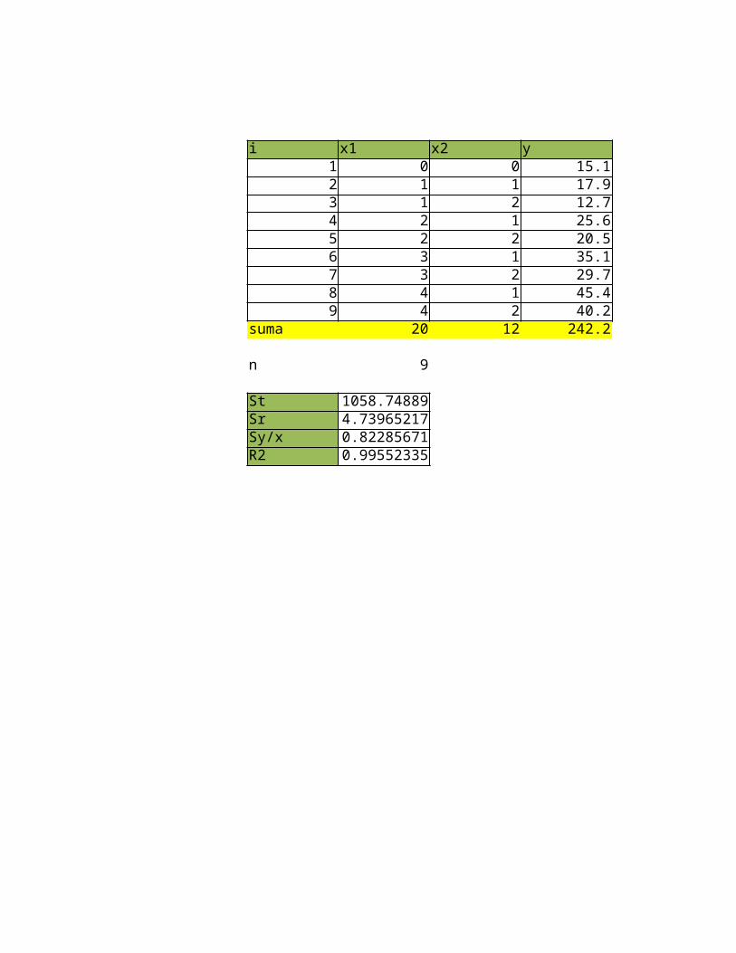
i x1 x2 y x1^21 0 0 15.1 02 1 1 17.9 13 1 2 12.7 14 2 1 25.6 45 2 2 20.5 46 3 1 35.1 97 3 2 29.7 98 4 1 45.4 169 4 2 40.2 16

suma 20 12 242.2 60

n 9

St 1058.74889Sr 4.73965217Sy/x 0.82285671R2 0.99552335

x1*x2 x2^2 x1y x2y (y-y^)2 (y-y-)20 0 0 0 0.40848771 139.5023461 1 17.9 17.9 0.01398563 81.20012352 4 12.7 25.4 0.38764159 201.9556792 1 51.2 25.6 1.45674405 1.719012354 4 41 41 0.36313724 41.10234573 1 105.3 35.1 0.53607864 67.05790126 4 89.1 59.4 0.18303516 7.777901244 1 181.6 45.4 0.2944242 341.8390128 4 160.8 80.4 1.09611796 176.594568

30 20 659.6 330.2 4.73965217 1058.74889

Matriz

a0 a1 a2 b b a19 20 12 242.2 242.2 20

20 60 30 659.6 659.6 6012 30 20 330.2 330.2 30

KramerDeterminante 460 Da0 6652

a0 14.4608696a1 9.02521739a2 -5.70434783

Formula 14.4608696 + 9.02521739 x + -5.70434783

a2 a0 b a2 a012 9 242.2 12 930 20 659.6 30 2020 12 330.2 20 12

Da1 4151.6 Da2

x2

a1 b20 242.260 659.630 330.2

-2624

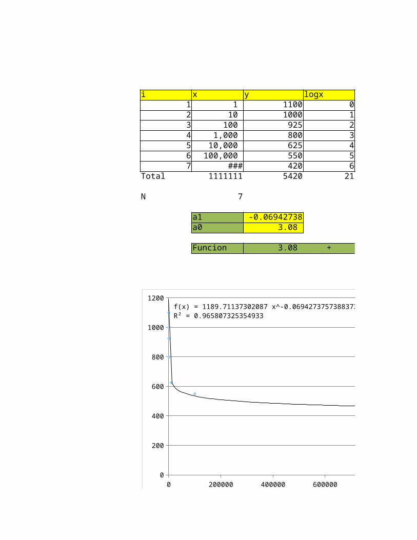
i x y logx1 1 1100 02 10 1000 13 100 925 24 1,000 800 35 10,000 625 46 100,000 550 57 1,000,000 420 6

Total 1111111 5420 21

N 7

a1 -0.069427376a0 3.08

Funcion 3.08 +

0 200000 400000 600000 800000 1000000 12000000

200

400

600

800

1000

1200f(x) = 1189.71137302087 x -̂0.0694273757388373R² = 0.965807325354933

Column DPower (Column D)

logy logxlogy x23.04139268515823 0 0

3 3 12.96614173273903 5.93228347 42.90308998699194 8.70926996 92.79588001734408 11.1835201 162.74036268949424 13.7018134 25

2.6232492903979 15.7394957 3620.0701164021254 58.2663827 91

beta -0.06942738 alpha 1,189.71

-0.0694273757388379 x

0 200000 400000 600000 800000 1000000 12000000

200

400

600

800

1000

1200f(x) = 1189.71137302087 x -̂0.0694273757388373R² = 0.965807325354933

Column DPower (Column D)

i x y1 0 672 4 843 8 984 12 1255 16 1496 20 185

0 5 10 15 20 250

20

40

60

80

100

120

140

160

180

200

f(x) = 5.8 x + 60R² = 0.975476387738194

Column DLinear (Column D)

0 5 10 15 20 250

20

40

60

80

100

120

140

160

180

200

f(x) = 0.150669642857143 x² + 2.78660714285714 x + 68.0357142857143R² = 0.997945762812167

Column DPolynomial (Column D)

0 5 10 15 20 250

20

40

60

80

100

120

140

160

180

200

f(x) = 67.3060364271902 exp( 0.0502932200598211 x )R² = 0.997865761161738

Column DExponential (Column D)

0 5 10 15 20 250

20

40

60

80

100

120

140

160

180

200

f(x) = 0.150669642857143 x² + 2.78660714285714 x + 68.0357142857143R² = 0.997945762812167

Column DPolynomial (Column D)

la cuadratica es la que se acopla mejor a los datos debido a la curvatura

0 5 10 15 20 250

20

40

60

80

100

120

140

160

180

200

f(x) = 5.8 x + 60R² = 0.975476387738194

Column DLinear (Column D)

0 5 10 15 20 250

20

40

60

80

100

120

140

160

180

200

f(x) = 0.150669642857143 x² + 2.78660714285714 x + 68.0357142857143R² = 0.997945762812167

Column DPolynomial (Column D)

0 5 10 15 20 250

20

40

60

80

100

120

140

160

180

200

f(x) = 67.3060364271902 exp( 0.0502932200598211 x )R² = 0.997865761161738

Column DExponential (Column D)

0 5 10 15 20 250

20

40

60

80

100

120

140

160

180

200

f(x) = 0.150669642857143 x² + 2.78660714285714 x + 68.0357142857143R² = 0.997945762812167

Column DPolynomial (Column D)

la cuadratica es la que se acopla mejor a los datos debido a la curvatura