Policy Research Working Paper 7662

Property Rights for Fishing Cooperatives

How (and How Well) Do They Work?

Octavio Aburto-Oropeza Heather M. Leslie

Austen Mack-Crane Sriniketh Nagavarapu

Sheila M.W. Reddy Leila Sievanen

Development Economics Vice PresidencyOperations and Strategy TeamMay 2016

WPS7662P

ublic

Dis

clos

ure

Aut

horiz

edP

ublic

Dis

clos

ure

Aut

horiz

edP

ublic

Dis

clos

ure

Aut

horiz

edP

ublic

Dis

clos

ure

Aut

horiz

edP

ublic

Dis

clos

ure

Aut

horiz

edP

ublic

Dis

clos

ure

Aut

horiz

edP

ublic

Dis

clos

ure

Aut

horiz

edP

ublic

Dis

clos

ure

Aut

horiz

edP

ublic

Dis

clos

ure

Aut

horiz

edP

ublic

Dis

clos

ure

Aut

horiz

edP

ublic

Dis

clos

ure

Aut

horiz

edP

ublic

Dis

clos

ure

Aut

horiz

edP

ublic

Dis

clos

ure

Aut

horiz

edP

ublic

Dis

clos

ure

Aut

horiz

edP

ublic

Dis

clos

ure

Aut

horiz

edP

ublic

Dis

clos

ure

Aut

horiz

edP

ublic

Dis

clos

ure

Aut

horiz

edP

ublic

Dis

clos

ure

Aut

horiz

edP

ublic

Dis

clos

ure

Aut

horiz

edP

ublic

Dis

clos

ure

Aut

horiz

edP

ublic

Dis

clos

ure

Aut

horiz

edP

ublic

Dis

clos

ure

Aut

horiz

edP

ublic

Dis

clos

ure

Aut

horiz

edP

ublic

Dis

clos

ure

Aut

horiz

edP

ublic

Dis

clos

ure

Aut

horiz

edP

ublic

Dis

clos

ure

Aut

horiz

edP

ublic

Dis

clos

ure

Aut

horiz

edP

ublic

Dis

clos

ure

Aut

horiz

edP

ublic

Dis

clos

ure

Aut

horiz

edP

ublic

Dis

clos

ure

Aut

horiz

edP

ublic

Dis

clos

ure

Aut

horiz

edP

ublic

Dis

clos

ure

Aut

horiz

edP

ublic

Dis

clos

ure

Aut

horiz

edP

ublic

Dis

clos

ure

Aut

horiz

edP

ublic

Dis

clos

ure

Aut

horiz

edP

ublic

Dis

clos

ure

Aut

horiz

ed

Produced by the Research Support Team

Abstract

The Policy Research Working Paper Series disseminates the findings of work in progress to encourage the exchange of ideas about development issues. An objective of the series is to get the findings out quickly, even if the presentations are less than fully polished. The papers carry the names of the authors and should be cited accordingly. The findings, interpretations, and conclusions expressed in this paper are entirely those of the authors. They do not necessarily represent the views of the International Bank for Reconstruction and Development/World Bank and its affiliated organizations, or those of the Executive Directors of the World Bank or the governments they represent.

Policy Research Working Paper 7662

This paper is a product of the Operations and Strategy Team, Development Economics Vice Presidency. It is part of a larger effort by the World Bank to provide open access to its research and make a contribution to development policy discussions around the world. Policy Research Working Papers are also posted on the Web at http://econ.worldbank.org. Corresponding author may be contacted at sri@acumenllc.com.

Devolving property rights to local institutions has emerged as a compelling management strategy for natural resource management in developing countries. The use of property rights among fishing cooperatives operating in Mexico’s Gulf of California provides a compelling setting for the-oretical and empirical analysis. A dynamic theoretical model demonstrates how fishing cooperatives’ manage-ment choices are shaped by the presence of property rights, the mobility of resources, and predictable environmental fluctuations. More aggressive management comes in the form of the cooperative leadership paying lower prices to cooperative members for their catch, as lower prices dis-incentivize fishing effort. The model’s implications are

empirically tested using three years of daily logbook data on prices and catches for three cooperatives from the Gulf of California. One cooperative enjoys property rights while the other two do not. There is empirical evidence in sup-port of the model: compared to the other cooperatives, the cooperative with strong property rights pays members a lower price, pays especially lower prices for less mobile spe-cies, and decreases prices when environmental fluctuations cause population growth rates to fall. The results from this case study demonstrate the viability of cooperative man-agement of resources but also point toward quantitatively important limitations created by the mismatch between the scale of a property right and the scale of a resource.

Property Rights for Fishing Cooperatives: How (and How Well) Do They Work?

Octavio Aburto-Oropeza, Heather M. Leslie, Austen Mack-Crane, Sriniketh Nagavarapu,

Sheila M.W. Reddy, and Leila Sievanen

JEL Codes: O13, Q20, Q22, Q50, Q56, Q57

Keywords: Cooperatives, fisheries, property rights, natural resources

Octavio Aburto-Oropeza is an assistant professor at Scripps Institution of Oceanography, University of

California-San Diego (maburto@ucsd.edu). Heather M. Leslie is director and Libra Associate Professor at Darling

Marine Center, University of Maine (heather.leslie@maine.edu). Austen Mack-Crane is a research assistant at the

Center on Social Dynamics and Policy, Brookings Institution (wmack-crane@brookings.edu). Sriniketh Nagavarapu

(corresponding author) is a senior policy associate at Acumen, LLC (sri@acumenllc.com). Sheila M.W. Reddy is a

senior scientist for sustainability at The Nature Conservancy (sreddy@tnc.org). Leila Sievanen is an associate scientist

at California Ocean Science Trust (leila.sievanen@oceansciencetrust.org). We appreciate outstanding research

assistance from Gustavo Hinojosa Arango, Juan José Cota Nieto, Alexandra Sánchez, Alexander Lobert, Florencia

Borrescio-Higa, Ashley Anderson, Steven Hagerty, and Katherine Wong. For invaluable advice, we thank Chris

Costello, Robert Deacon, Andrew Foster, Vernon Henderson, Kaivan Munshi, and seminar participants at Brown’s

Population Studies and Training Center, Brown’s Spatial Structures in the Social Sciences, the UC-Santa Barbara

fisheries working group, the MIT/Harvard Environment and Development seminar, and the UC-Berkeley ARE

seminar. We are grateful for financial support from the Institute at Brown for Environment and Society at Brown

University and the US National Science Foundation Coupled Natural and Human Systems program (NSF Award GEO-

11114964). Remaining errors are our own. Author contributions: 1) Design of research: Leslie, Nagavarapu, Reddy; 2)

Quantitative data: Aburto, Reddy; 3) Qualitative data: Leslie, Reddy, Sievanen; 4) Theoretical model: Mack-Crane,

Nagavarapu; 5) Empirical analysis: Mack-Crane, Nagavarapu, Reddy; 6) Writing: Leslie, Mack-Crane, Nagavarapu,

Reddy.

2  

There is widespread concern for the health of global fisheries: a recent study estimated that 28–

33% of fisheries are over-exploited and 7–13% are collapsed (Branch et al. 2011).1 Since Gordon

(1954) and Scott (1956), the static and dynamic externalities that lead to over-extraction have been

well understood. However, policy makers and researchers have struggled with how best to ensure

that these externalities are properly internalized, particularly in low-income countries. In this paper,

we use a blend of theory and empirics to better understand whether, when, and how assigning

property rights to fishing cooperatives can resolve the externality problem.2

Assigning cooperatives the exclusive right to fish a spatially delineated area—a specific

case of a Territorial Use Right Fishery (TURF) (see Wilen et al. 2012)—is an attractive concept. It

potentially improves upon much more common solutions to the externality problem, such as catch

shares, tradable quotas, and marine reserves (Hilborn et al. 2005; Deacon 2012). While these more

common systems have been associated with improved ecological and economic outcomes (Hilborn

et al. 2005; Costello et al. 2008; Lester et al. 2009), they require intensive monitoring and

enforcement that may be relatively costly. In contrast, cooperatives may be able to leverage social

ties to monitor and enforce spatial boundaries at relatively low cost. Moreover, cooperatives can

allocate fishing effort across space and time in a manner that avoids both closing a fishery and the

race for especially profitable fishing areas or times that is inherent with transferable quotas. A

cooperative’s ability to coordinate its members’ actions could also reduce races to fish within a

TURF that is assigned to a less cohesive group of fishers (Costello and Kaffine 2010). Finally, a

cooperative could facilitate greater provision of public goods that reduce members’ private fishing

costs, such as information on the best fishing locations or shared equipment.

Despite these advantages, there are still two major challenges to the effective use of

property rights by fishing cooperatives, and empirical evidence on these challenges is scarce. First,

the scale of the property right may not match the scale of the resource, thereby giving a cooperative

much less incentive and ability to manage its exclusive rights (Ostrom 1990; White and Costello

2011).3 The “scale of the resource” refers to the degree of geographic mobility of the organisms

targeted by fishers. Second, and less often discussed in the literature, cooperative management may

                                                       1. “Over-exploited” refers to stocks less than half of maximum sustainable yield (MSY), while “collapsed” is defined as stocks less than one-fifth of MSY. 2. Following Deacon (2012), we define fishing cooperatives as “an association of harvesters that collectively holds rights to control some or all of its members’ fishing activities.” Cooperatives are quite common; for example, Deacon (2012) points to at least 400 cooperatives in Bangladesh and over 12,000 in India. 3. A similar problem arises if a local user group does not have control over a species that is ecologically connected to the resource it controls. For instance, fishermen outside the group may fish species that are preyed on by species controlled by the group.

3  

not adapt effectively in the face of environmental variability. For instance, cooperatives may need

to ensure members some minimum level of well-being in order to retain members; this may hinder

a cooperative’s ability to dramatically cut fishing effort when environmental conditions negatively

impact fish populations.

In this paper, we develop a dynamic model of cooperative decision-making and use rich

data from Mexico’s Gulf of California fisheries to examine how fishing cooperatives exercise

property rights, with a focus on three issues: 1) Whether cooperatives with property rights manage

a resource differently from those without; 2) How such differences depend on the scale of the

resource; and 3) How such differences respond to predictable environmental fluctuations associated

with ENSO (El Niño/Southern Oscillation) events. Mexico is a natural setting for the analysis. The

country’s marine ecosystems are rich in biodiversity, which provides an opportunity to examine

how fishing cooperatives shift behavior when fishing on species that vary in key traits, such as

mobility. Moreover, ENSO events have important impacts on fisheries, with the direction and

magnitude of these impacts differing among species.

We begin our analysis with a dynamic model of cooperative decision-making. Cooperative

leadership can engage in more aggressive management by lowering the price that is paid to

cooperative members for a specific species and, therefore, disincentivizing fishing of that species.

The model yields three testable implications for how cooperative price and resulting catch change

in response to external factors. Specifically, compared to other cooperatives, a cooperative with

stronger property rights manages effort more aggressively, decreases the relative aggressiveness of

management if a species is highly mobile, and restricts effort more when environmental forcing

(e.g., ENSO events) limit the population growth rate of a species. Throughout, by “strong property

rights” we mean the ability to exclude noncooperative fishers from the cooperative’s established

fishing grounds.

We test these implications using daily logbook data from three cooperatives in the Gulf of

California region, in northwest Mexico. One cooperative, operating on the Pacific coast, retains an

exclusive concession for some species and is able to exclude outside fishermen for all other species

(Cota-Nieto 2010; McCay et al. 2014). The other two cooperatives are located close to La Paz, the

state capital of Baja California Sur (B.C.S.), and compete with other cooperatives and

noncooperative fishermen for fish (Basurto et al. 2013; Sievanen 2014). Analysis using the fishing

team-level logbook data reveals that cooperative members respond to cooperatives’ chosen prices

as posited by the model. Exploiting the fact that one cooperative has stronger property rights than

4  

the other two, we use the cooperative-level price and catch data to demonstrate empirical support

for the model’s three implications. The difference in price and catch between the cooperative with

strong property rights and the other two cooperatives is large, and the cooperative with property

rights disincentivizes effort more aggressively than the other two when growth rates are likely to be

small. But the magnitudes of the estimates also indicate that the difference in management

aggressiveness across the cooperatives shrinks in economically meaningful ways when resource

scale is large and growth rates are high.

Given the small number of cooperatives in the analysis, one should be cautious in

extrapolating these findings to other settings. Instead, we view our results as improving the general

understanding of when and how cooperative-based property rights can be effective. Our work

complements the rich literature on community-based resource management institutions. Ostrom

(1990) reviews case studies of institutions and derives a set of principles that differentiate those

that are successful. We examine the role of some key principles from the Ostrom framework, such

as clearly defined boundaries and effective rule enforcement. However, rather than making binary

assessments of “success,” we empirically quantify the influence of property rights on economic

outcomes. Gutiérrez et al. (2011) consider case studies of fishing cooperatives in particular and

find predictors of success, including the existence of quotas, enforcement institutions, long-term

planning, and resource mobility. Recent economics literature examines the decision-making of

villages or other local user groups regarding other resources (e.g., Edmonds [2002] and Foster and

Rosenzweig [2003] on forests). In contrast to these studies, we examine the short-term dynamics of

resource management, illuminating the mechanisms that institutions may use to achieve

management goals. We do so in the context of fisheries, which are characterized by important

spatial externalities and environmental fluctuations not relevant to some other natural resources.

The theoretical literature on optimal fisheries management strategies considers these

challenges. For instance, Costello and Kaffine (2010) and White and Costello (2011) examine the

implications of spatial externalities in area-based property rights, driven by movement of species

across large ranges. Reed (1975), Parma and Deriso (1990), Costello et al. (2001), and Carson et al.

(2009) look at how management may respond to temporary or permanent environmental changes.

Our paper examines similar issues but introduces an important complication arising from

cooperative leaders’ need to ensure returns high enough to retain members. More importantly, our

focus is on empirically testing our theoretical model and presenting quantitative evidence on

cooperative decision-making.

5  

Three important, recent papers examine fishing cooperatives empirically. Deacon et al.

(2008) and Deacon et al. (2013) develop a model incorporating concerns specific to cooperatives

and then empirically test this model. They examine the intraseasonal allocation of fishing effort

across space, time, and fishers in a salmon fishery with one cooperative and independent fishers.

Our work provides less detail on the location of fishing effort and instead focuses on the allocation

of effort across time in the face of species-specific differences in mobility and large-scale

environmental oscillations that cycle over several years. Ovando et al. (2013) use a survey of 67

cooperatives from around the world to examine what management tools cooperatives use and how

this is shaped by differing economic, political, and ecological contexts. We focus on a particular

management instrument—the choice of what price to pay cooperative members—and we

complement our empirical analysis with a detailed theoretical model that delivers clear predictions

for how this instrument should respond to a variety of circumstances.

The paper proceeds as follows. Section 1 describes the setting of Mexico’s fisheries in more

detail. Section 2 describes the data used in the empirical analysis. Section 3 develops the theoretical

model and derives three testable implications. Section 4 uses the model to develop empirical tests

of these implications and presents empirical results from these tests. Section 5 concludes.

I MEXICO’S GULF OF CALIFORNIA FISHERIES

Bordering five Mexican states, the Gulf of California is one of the most biologically

productive areas of the world’s oceans.4 While the region’s remarkable biodiversity has

considerable conservation value, it also is of substantial social and economic importance. The

states surrounding the Gulf contribute 71% of Mexico’s total fisheries volume and 57% of total

value (OECD 2006). As in many parts of the world, the Gulf’s fleet is characterized by small-scale

subsistence or commercial fishing on small two or three-person boats. Small-scale fisheries are a

major source of employment and income, as well as a safety net in times of economic or

environmental uncertainty (Pauly 1997; Allison and Ellis 2001; Basurto and Coleman 2010).

However, a number of commercially valuable species have declined in recent years due to several

factors, including improved technology, population and income growth, and increased export

opportunities (Sala et al. 2004; Sáenz-Arroyo et al. 2005; Dong et al. 2004).

Several ecological factors make the Gulf of California an appropriate focus for our study.

The species targeted by small-scale fishers have diverse life histories, ranging from those with

                                                       4. In addition to the Gulf proper, here we also consider the Pacific Coast of B.C.S. as part of the “Gulf region,” in keeping with previous work as in COBI/TNC (2006).

6  

fairly high site fidelity (e.g., lobster [Acosta 1999]) to those that move extensively as larvae (e.g.,

shrimp [Calderon-Aguilera et al. 2003]) or adults (e.g., tuna [Schaefer et al. 2007]). This variation

allows for an analysis of how cooperatives deal differently with species that vary in their mobility.

Moreover, the region’s terrestrial and marine ecosystems respond dramatically to ENSO (El

Niño/Southern Oscillation) events, which occur every several years (Polis et al. 2002; Velarde et al.

2004). During El Niño years, ocean waters warm, upwelling slows, and rainfall increases, with

important implications for fisheries species (Velarde et al. 2004; Aburto-Oropeza et al. 2007).

While ocean productivity varies temporally—both with ENSO and other sources of climatic

variability—and spatially throughout the Gulf region, we find remarkable coherence in the

variability of mean concentration of chlorophyll a, a common proxy for marine primary

productivity (Mann and Lazier 2005) in the vicinity of the three cooperatives for which we have

logbook data (Leslie et al. 2015). ENSO’s significant role enables us to explicitly test the influence

of periodic environmental shocks on cooperatives’ decision-making. ENSO may affect species

through three channels: recruitment and growth of juveniles, growth of adults, and movement of

adults. Here we focus on the recruitment channel.

Fishing cooperatives have had a long history in the Gulf of California—and Mexico more

broadly—and continue to be a major factor in the fishing industry today. Under the 1947 Fisheries

Law, cooperatives had exclusive concessions to the eight most commercially valuable species and

often had rights to bays, estuaries, or lagoons adjacent to their lands (DeWalt 2001; Young 2001).

In addition to cooperatives, the fisheries law created two other classes of fishermen:

permisionarios, who are private individuals or corporate entities with permits to catch—and sell to

the open market—species for which cooperatives do not hold concessions; and pescadores libres,

who have rights to fish within cooperatives’ concessions for subsistence only, but are also allowed

to fish for permisionarios (Young 2001).

To encourage private investment in fisheries, the 1992 Fisheries Law took exclusive rights

for the eight species away from the cooperatives and made it possible for permisionarios to fish

and sell them (SEPESCA 1992; Ibarra 1996; Villa 1996; Ibarra et al. 1998; Ibarra et al. 2000;

Young 2001). Consequently, in the present-day system, independent fishers (i.e., permisionarios)

are able to fish most species and sell their catch as long as they are able to acquire permits to do so.

The acquisition of these permits involves important costs, including the administrative burden of

applying for a permit, interactions with government officials, travel to (often distant) administrative

offices, and the financial cost of the permit itself.

7  

Despite this change, fishing cooperatives continue to play an important role in these

fisheries. Our review of the literature, field visits, and conversations with researchers at Centro

para la Biodiversidad Marina y la Conservacion (CBMC) have revealed that cooperative

membership entails a series of restrictions on behavior, a specific form of compensation, and a

potentially attractive set of benefits.

In terms of restrictions on behavior, cooperative members are more constrained than those

fishers who are not cooperative members. They are nominally bound to the rules of the

cooperative, which determine how, when, and where to fish (see Reddy et al. 2013). A one-time

membership payment and an agreement to sell only to the cooperative are also typical (J. J. Cota

Nieto, pers. com., 2014). While enforcement of these restrictions varies among cooperatives, social

ties may aid in enforcement. Cooperative membership requirements vary, both contemporaneously

and historically, but typically, cooperative members live in the community and are often sons of

prior members (e.g., Petterson 1980).

Cooperative membership also entails a specific form of compensation. Cooperative leaders

will negotiate with a buyer to supply a certain amount of product. They then set a price and

quantity for that species and pay those fishers who return with product that price, which is some

fraction of the market price (Reddy et al. 2013; J. J. Cota-Nieto, pers. com., 2014). Importantly,

prices are used in combination with direct restrictions or quotas. Cooperative leaders have a sense

of what price is required to fill a quota and can lower the price to avoid incentivizing fishing past a

quota (G. Hinojosa-Arango, pers. com., 2014). In this sense, the price paid to cooperative members

by the cooperative leaders is one form of controlling the effort of cooperative members.

Cooperative leaders can use prices as a management tool, in addition to more direct restrictions, to

help ensure a certain amount of fishing effort and, ultimately, catch.

Given that the price paid to cooperative members is below the market price, the cooperative

accrues revenue that can be used to generate various benefits of cooperative membership. This

revenue is used to pay administrative costs that aid the cooperative as a whole, which include the

salaries of cooperative officials, travel and legal expenses, and taxes (McGuire 1983). Benefits to

members from these administrative efforts include access to fishing permits, gear, state subsidies,

and shared resources for processing, marketing, and reporting catch (Petterson 1980; Basurto et al.

2013; McCay et al. 2014; Sievanen 2014). Access to permits is one of the primary reasons for

joining a cooperative, according to La Paz area fishers (e.g., Sievanen 2014), and thus, those fishers

who do not have the financial or social capital to acquire permits as individuals (as the

8 

permisionarios do) are more likely to join cooperatives. Revenue may be paid out in annual

bonuses, which may be based on fishermen’s total annual catch, equal for all members, or

determined by some other rule (McGuire 1983). Finally, in some cooperatives, members also enjoy

income security through sources such as retirement benefits or credit (McCay et al. 2014; G.

Hinojosa-Arango, pers. com., Feb. 2012).

In the theoretical model below, we model these benefits received by cooperative members

in two ways: (i) a lump sum payment reflecting discounts on equipment (including boats and

motors), credit, or annual bonuses from the cooperative leadership; (ii) a factor reducing the costs

of fishing reflecting access to fishing permits and state subsidies for fuel, as well as the absence of

costs associated with searching for buyers. To the extent that the size of an annual bonus is

dependent on annual catch, the bonus is not appropriately classified as a lump sum payment, as it

affects incentives for effort. We do not have information on how often such catch-dependent

bonuses occur, but it is important to note from the above discussion that other forms of

compensation also make up the lump sum payment.

While the features above are generally shared by many cooperatives in the Gulf of

California area, there are key differences among the three cooperatives for which we have daily

logbook data and conduct empirical analysis. Figure 1 shows the location of these cooperatives.

Pichilingue is located on the outskirts of La Paz, the largest city in the state and a major market in

the region, and Sargento is a short drive away from La Paz. Punta Abreojos, a member of the

federation of cooperatives in Northwest Baja California known as FEDECOOP, is on the Pacific

side of the peninsula, adjacent to other cooperatives from FEDECOOP. For the purposes of the

empirical work below, we utilize the fact that Abreojos effectively has more secure property rights

than Pichilingue and Sargento and can therefore manage its own members and restrict access for

nonmembers more easily.

This arises for five reasons. First, Abreojos fishes in a relatively isolated area, while

Pichilingue and Sargento fish in areas that have many cooperatives and fishers (McCay et al.

2014). There is a larger pool of potential fishers for Pichilingue and Sargento to compete with.

Second, Punta Abreojos and the other cooperatives in FEDECOOP successfully retained exclusive

fishing rights to lobster, abalone, snails, and a few other species even after 1992 (McCay et al.

2014; Cota-Nieto 2010; J. J. Cota-Nieto, pers. com., May 2012). The ten cooperatives in

FEDECOOP each have separate, clearly defined polygons in which no other cooperative of

FEDECOOP and no non-FEDECOOP fisher can fish these species, unless it is for subsistence

9  

purposes. Third, even though these polygons were originally designed for the species with

exclusive concessions, in practice they provide clear boundaries for other species as well (Cota-

Nieto 2010). Cooperatives with adjacent polygons may fish for species without exclusive

concessions in the neighbor’s polygon, but this typically involves negotiated agreements between

the leaders of the two cooperatives involved (J. J. Cota-Nieto, pers. com., May 2015). Fourth,

FEDECOOP has created a system in which fishers in each of the member cooperatives are

expected to spend a fraction of their time in monitoring and vigilance efforts to enforce spatial

restrictions (McCay et al. 2014). Fifth, FEDECOOP members can be removed from their

cooperatives if they fail to sell exclusively to their cooperative or fail to comply with other rules

(McCay et al. 2014). The lost benefits from eviction could be much more substantial for Abreojos

than for the La Paz cooperatives because of the consistently high value of FEDECOOP fisheries

(ensured by productive waters, local monitoring, FEDECOOP’s employment of fisheries scientists,

and FEDECOOP’s engagement with the state) (McCay et al. 2014). While exclusive sale to the

cooperative may be a nominal requirement for La Paz area cooperative fishers, the cooperative

leadership in La Paz do not have the same degree of control of their members to ensure that sales of

product outside the cooperative do not occur (J. J. Cota Nieto, pers. com., May 2014). To be sure,

illegal fishing still occurs in the areas fished by the FEDECOOP cooperatives, but for these five

reasons the scale of illegal fishing is likely to be less on the Pacific side of the Gulf. We therefore

view Abreojos as an “exclusive” cooperative and Pichilingue and Sargento as “nonexclusive”

cooperatives for the purposes of testing our hypotheses below.

Finally, it is important to understand whether any given fisher or cooperative can influence

the market price of fish through their catch decisions. There are a large number of fishers in the

area. As of 2010, based on data compiled by the National Commission of Aquaculture and Fishing

(CONAPESCA), the number of fishers in La Paz alone was estimated at 974 people (748

cooperative members plus 226 unregistered fishers) (Leslie et al. 2015). According to data

collected from La Paz fish markets by researchers from CBMC and the Scripps Institution of

Oceanography, the three cooperatives we studied (Punta Abreojos, Pichilingue, and Sargento) were

estimated to each provide approximately 12%, 5%, and 8%, respectively, of the fisheries product

sold in the La Paz market (Sanchez, Nieto, Osorio, Erisman, Moreno-Baez, and Aburto-Oropeza

2015). Abreojos is more focused on the export market, however. These numbers come from an

effort to enumerate the major players in La Paz markets and may be an over-estimate as smaller

sellers are not easy to find. The size of the market shares suggest that these cooperatives will have

1 

some market power, but we believe the shares are small enough that this is not a first-order

concern.

II DATA AND DESCRIPTIVE STATISTICS

The empirical analysis uses daily logbook data from the three fishing cooperatives noted

above, Pichilingue, Sargento, and Abreojos. Daily data on catches from fishing teams in each

cooperative were recorded from January 1, 2007, to December 31, 2009. Catch records include a

team identifier (for Abreojos and Pichilingue only), the common name of the species caught, the

weight of the catch (kilograms), and price per kilogram offered by the cooperative (pesos). The

composition of the species fished by the cooperatives partially reflects the biogeography of the

Pacific vs. the Gulf coast of B.C.S.; however, there is still substantial overlap, thereby allowing a

comparison of the behavior of the different types of cooperatives for a given species.

The logbook data have information on the prices cooperatives paid to their fishermen but,

unfortunately, do not have information on the price the cooperative sold the catch at in the market.

Using the Sistema Nacional de Informacion e Integracion de Mercados (SNIIM), available from

the Mexican government, we have collected data on daily market prices in La Paz for as many

species and dates as possible.5 Using the dates in the cooperative logbooks, these market prices are

matched to the cooperative purchases. In cases where a market price is not available for a particular

date, the average price for the corresponding week or month is substituted instead (depending on

availability).

To examine whether market prices in La Paz are driven by external forces that are

exogenous to supply factors in the vicinity of La Paz, we use the SNIIM to obtain market prices

from La Nueva Viga, a large national fish market in Mexico City connecting sources to

distributors. The La Nueva Viga data contain information on marine fish, crustaceans, freshwater

fish, and mollusks/others. B.C.S. is listed as a source only for the fourth category. This, coupled

with the fact that other sources of La Nueva Viga catch have only a partial overlap of species with

La Paz, limits the number of species that can be matched to the logbook data. In cases where a

market price is not available for a particular date in the logbook, the average price for the

corresponding week or month is again used. All cooperative and market prices are converted into

2010 Mexican pesos using a Consumer Price Index obtained from the OECD.

We aim to understand how cooperative pricing responds to natural variation that alters

population growth rates. The Oceanic Niño Index (ONI) is a three-month running mean of an

                                                       5. Available at http://www.economia-sniim.gob.mx/i_default.asp.

1 

underlying measure of ENSO cycles, which alter ocean temperature. Data on ONI are publicly

available from the National Weather Service Climate Prediction Center.6 These data are matched to

every cooperative purchase in the logbook data. The second half of 2007 and first half of 2008

were marked by a “cold episode” (more negative values), while the second half of 2009 saw the

onset of a “warm episode” (more positive values).

Warmer ocean temperatures have three potential effects on organisms. First, they negatively

affect juvenile recruitment of some species and positively affect recruitment of others. These

population growth rate effects ultimately impact catch with a lag that generally ranges from one to

seven years. Second, warmer temperatures can either positively or negatively affect adult

population abundance by causing individuals to migrate. Third, adult size may be affected through

changes in individual growth. The model focuses on population growth rates and does not

incorporate the other two effects for the sake of tractability. Therefore, the empirical tests also

focus on the first effect.

Finally, we conducted a thorough review of the ecological literature to construct a detailed

classification of species on two dimensions. First, we classify species as “large scale” (i.e., large

scale of movement, or highly mobile) or “small-scale” (i.e., small scale of movement, or less

mobile). This classification is based primarily on knowledge of the movement of adult organisms,

rather than on knowledge of larval dispersal. Second, we create a variable equal to 1 if higher ONI

has a positive effect on recruitment (and hence population growth rates) and equal to -1 if higher

ONI has a negative effect on recruitment. If the effect on recruitment is unknown to us or if there is

no effect on recruitment, we set the variable to 0.

Table 1 provides summary statistics on the final merged data set.7 The first panel shows

summary statistics for the three cooperatives together, the second panel shows statistics for

Pichilingue and Sargento only, and the third panel shows statistics for Abreojos only.

While the logbook data is at the individual fishing transaction level, the data are aggregated

in our tests of the model’s implications to the species-year-month-week level by averaging prices

and totaling catch. This is because our own field visits suggested that cooperatives do not usually

                                                       6. Available at http://www.cpc.noaa.gov/products/analysis_monitoring/ensostuff/ensoyears.shtml. 7. Observations where the market price is less than the cooperative price are dropped due to concerns about measurement of market prices. This affects only 762 transactions out of approximately 42,000 individual fishing transactions for which we have cooperative price data.

1 

alter prices on a day-to-day basis.8 Therefore, in all three tables of descriptive statistics, an

observation is at the aggregated level.

There is a significant amount of variation in total catch, market prices, and cooperative

prices (table 1). Comparing the second and third panels of table 1, the log of cooperative price and

log of total catch show a marked difference between the exclusive and nonexclusive cooperatives,

despite the fact that average market prices are similar. The log of cooperative price and the log of

catch also have a higher coefficient of variation for the exclusive cooperative.

The final rows of each panel show the range of variation for the “Recruit Effect” variable

and the “ONI X Recruit Effect” interaction. The majority of observations have a value of 0 for the

“Recruit Effect” variable, but approximately 800 observations exhibit a positive recruitment effect,

and more than 500 observations exhibit a negative effect (figure 2). This variation permits a test of

the model’s third implication regarding population growth rates.

To understand the relationship between market prices in La Paz and market prices external

to that fishing area, we use the daily transaction data to estimate a regression of La Paz prices on

La Nueva Viga prices, separately for each species for which there are data from both sources. Of

the 55,841 daily transactions across Abreojos, Sargento, and Pichilingue, the species that match

across the logbooks and La Nueva Viga account for only 4,208 transactions. Moreover, some of

these transactions have no information on La Paz market prices. In table 2, we run OLS regressions

of the log La Paz price on the log La Nueva Viga price by species common name.

The results paint a mixed picture. For five of the nine common names, there is a positive

and statistically significant relationship between La Nueva Viga prices and La Paz prices. For

these, the R-squared ranges from 0.016 to 0.877, depending on the species. Two of the nine

common names have coefficients that are not statistically distinguishable from zero. The remaining

two common names have negative and statistically significant relationships. Moreover, these

relationships are not simply an artifact of La Nueva Viga sourcing particular species from La Paz.

Of the four species that are sometimes sourced from B.C.S. in the data (almeja, calamar, ostion,

and pulpo), three have a positive coefficient while one has a negative and significant coefficient. Of

the species not sourced from B.C.S., two have a positive coefficient, with cazon having especially

high representation in the logbook data. While this exercise is starkly limited by data challenges, it

suggests that the prices for some species are not just locally determined in La Paz.

                                                       8. Based on daily transaction data, we do sometimes observe multiple prices paid for a given species on a particular day. It is difficult to know whether this is measurement error or variation in price due to differences in time of day (e.g., a higher price for a more inconvenient time).

1 

III THEORETICAL MODEL

We first provide an overview of the model and then lay out the details in separate

subsections below. We consider a single-species fishery with one cooperative and a continuum of

fishers who are characterized by heterogeneous fishing costs. Each time period in the model is

divided into two stages. In the first stage, the cooperative chooses a per unit price cP to pay

cooperative members for their catch. The cooperative buys catch from its members at a price cP

and sells that catch on the market at a higher price mP . The retained earnings are used to pay for

operating costs, pay cooperative leadership, and provide lump-sum transfers back to cooperative

members. In the second stage, individual fishers decide whether or not to be in the cooperative, as

well as how much fishing effort to exert. Cooperative members can only sell to the cooperative; if

they want to sell to the open market, they must leave the cooperative. This gives the cooperative a

limited amount of monopsony power.9

The fundamental tradeoff facing the cooperative is that it can increase future stocks by

decreasing cP in the current period (and thereby disincentivizing current effort); but this will lower

current earnings and—in the case of a cooperative without exclusive fishing rights—induce some

fishers to leave the cooperative and fish independently.

We make four crucial, additional assumptions in the model. First, individual fishers are

atomistic: just as individual consumers and producers take market prices as given in the standard

competitive model, each individual fisher takes aggregate fishing effort across all fishers and

fishery stock as given. Pursuing a model in which individual fishers engage in strategic

considerations would be an interesting extension, but we use the simpler approach because of the

large number of individual fishers in these fisheries. In addition, the simplification allows for a

focus on the basic tradeoff facing the cooperative.

Second, we find an equilibrium in which the highest cost fishers sort into the cooperative.

Importantly, low costs in the model represent not just fishing skill, but also how easy it is for

fishers to acquire permits for catch, transport catch to market, and purchase fuel and other

equipment. Fishers who join the cooperative can lower their costs because the cooperative can

acquire permits, transport all catch to market and find buyers, share gear, and coordinate harvesting

                                                       9. In practice, cooperative members could also fish outside the cooperative, against the cooperative’s wishes. This is likely limited in the three cooperatives used in our analysis, but could definitely be a concern for other cooperatives. Our only goal is to illustrate the influence of fishers’ decisions to fish independently versus fish with the cooperative on the cooperative’s decisions, and we introduce this feature in the simplest way possible.

1 

activities (Ovando et al. 2013). The cost formulation below has the property that high cost

fishers obtain a greater benefit from these cooperative activities.

Third, fishers can costlessly move in and out of the cooperative. This assumption, in

combination with the assumption of atomistic fishers and no labor-leisure tradeoff for fishers, will

ensure that fishers choose whether or not to be in the cooperative in any period t based on a simple

comparison of profits in the cooperative versus outside the cooperative in period t alone.10 This

substantially simplifies the dynamic problem. Our work in the study areas suggests that it is not in

fact costless to move back and forth between cooperative and independent fishing, but we believe

the mathematical simplification makes this assumption worthwhile and keeps the focus on our

issue of primary concern: how the cooperative trades off between current returns and conservation

and how this is affected by the economic and environmental setting.

Fourth, we assume that market prices do not depend on the cooperative’s decisions. As

noted above, the cooperatives in our data are important players in the La Paz market, but none of

their market shares are above 12%. There is also evidence above that some of the prices in the La

Paz market are driven in important ways by external forces, though those results vary markedly by

species and speak to only a fraction of the species caught by our three cooperatives.

The following subsections lay out the details of the model and then develop three testable

implications.

The Evolution of Stock

There are both static and dynamic externalities associated with a fisher exerting more effort

in a particular time period. The “static” externality comes from the fact that when a fisher increases

effort today, he decreases the ease with which other fishers can harvest from today’s stock. The

“dynamic” externality comes from the fact that when fishers exert effort today, they reduce the

available stock in future periods. We formulate a simple model that captures both externalities.

As in Deacon et al. (2013), we assume that each unit of fishing effort extracts a fixed

proportion of the remaining stock. This does not depend on whether a fisher is fishing

individually or in a cooperative. If tX is the initial stock at the beginning of the period, the stock

after aggregate effort tH has been applied across all fishers is (1 )Ht

tX , and the overall quantity

extracted is = (1 (1 ) )Ht

t tQ X . Fishers extract simultaneously, and fisher i receives catch itq in

                                                       10. The model also implicitly assumes that fishers cannot save. This assumption will affect the model only if there is a labor-leisure tradeoff. Without a value for leisure, fishers with savings vehicles would still choose cooperative membership and hours to maximize profits in every period separately.

1 

proportion to his effort ith : = itit t

t

hq Q

H. Both an individual’s catch and the marginal return to an

individual’s fishing effort is decreasing in the effort of all other fishers.11

Next, we specify how current stocks and harvests translate into future stocks. Two common

choices are the Ricker model and the Beverton-Holt model. In both formulations, harvest and stock

growth are sequential: The initial stock in a period is harvested, and the remaining population leads

to the new stock. Researchers typically use the Beverton-Holt model in settings where recruitment

is relatively insensitive to population size because of density-dependent mortality (Clark 1990,

207–9). Since we would like harvest to have important effects on stocks, we instead use the Ricker

model (Clark 1990, 199, 202): 1 1(1 )

1 1= ( )X Qt trt K

t t tX X Q e

, where tr denotes an intrinsic rate of

growth and K is the carrying capacity.12 Substituting in the expression for aggregate catch yields

the following equation for the evolution of stock as a function of effort:

1(1 ) 1(1 )1

1= (1 )

Ht XtrH tt Kt tX X e

(1)

We do not use the most common fishery model, the Gordon-Shaefer model.13 We are

interested in the dynamic trajectory of prices and harvest toward steady state, and finding an

analytical expression for the optimal trajectory is generally not possible when we complicate the

cooperative’s problem by introducing a joining decision. This forces us to use a numerical solution

procedure, so it is natural to use a discrete time stock-recruitment model. Fortunately, Eberhardt

(1977) shows that the Ricker growth model is mathematically related to the standard continuous

                                                       

11. The derivative of fisher i’s catch with respect to all others’ effort is =i i

i i

q h Q Q

H H H H

. The term in

parentheses is negative, as can be shown by using a second-order Taylor series expansion of (1 )H about H=0. To

sign the cross-partial, take the derivative of i

i

q

H

with respect to ih . Re-arranging terms shows that the cross-partial

is 2

2i i

i i i

H hh Q Q Q

H h H H H H

, which is clearly negative if i iH h .

12. Under some choices of tr and K, this function can lead to limit-cycle oscillations without steady convergence to

any stable equilibrium when there is no harvesting. Our choices of parameters in the numerical simulations ensure this does not occur (Clark 1990, 202). 13. The Gordon-Shaefer model is a continuous time model in which the growth in stock follows the differential

equation = (1 )dX X

rX HXdt K

, where H is harvesting effort, K is carrying capacity, r is the intrinsic growth

rate, and is a parameter governing the return to effort.

1 

time logistic growth model under certain additional assumptions. Moreover, our way of expressing

the static externality is related to the discrete time analog of the Gordon-Shaefer harvest function.14

Individual Fisher and Cooperative Optimization Problems

We assume that in any period 0t , fisher i chooses 0= ,...,t t T , whether to be in the

cooperative sector ( = 1itD ) or not ( = 0itD ) and what hours to work in the cooperative sector ( itCh )

or the independent sector ( itIh ). In doing so, she takes current and future cooperative and market

prices as given. She solves the problem:

2

, , =0

2

1(1 (1 ) ) (1 )max

1(1 (1 ) )

THt itI t

mt t itI ith h D titI itC it t i

Ht itC tct t itC t it

t i

hP X h D

H

hP X h S D

H

where is the discount rate, mtP is the market price, ctP is the cooperative price, tH is total effort,

and tS is a lump-sum payment from the cooperative based on the revenue it accrues from the

difference in the market price and the cooperative price. Cooperative fishers are atomistic and

therefore take tH as given, in addition to prices. This will imply that they take tS as given. (We

state how tS is related to prices, stocks, and aggregate effort below in the cooperative’s problem.)

Heterogeneity across fishers comes through i , which denotes the inverse of the cost of effort for

fisher i. If the fisher remains independent, the cost function is 21=itI itI

i

c h

. If, instead, fisher i joins

the cooperative, the cost function is 21=itc itC

i

c h

, with > 0 . represents the reduction in

costs derived from fishing inside the cooperative.

The cooperative maximizes the present discounted value of current and future harvests from

period 0 to period T, minus the present value of members’ costs from period 0 to period T:

* 2

=0

1( ) [ ( )] ( ) dmax

( )

Tt

mt ct ct itC ct i ii coopP tct i

P Q P h P g

                                                       14. Assuming that harvest and stock growth are sequential and focusing on a constant harvest H for the period t–1 to t,

solve the differential equation =dX

HXdt

for X(t). The solution implies ( ) = ( 1)HX t e X t . This is

equivalent to our (1 ) ( 1)H X t for some (0,1) .

1 

where is the discount rate, ( )ct ctQ P is the aggregate catch by cooperative members as a function

of the cooperative price, * ( )itC cth P is the optimal effort choice of each member as a function of the

cooperative price, and ( )ig is the probability density function of i . We assume that i has an

exponential distribution: ( ) = iig e

. The term i coop indicates that the integral is taken over

those who choose to be members. When solving the model below, we will show that fishers with

i below a threshold *t will select into the cooperative, and this threshold is a function of ctP .

Total quantity caught by the cooperative is:

= (1 (1 ) )Hct t

ct tt

HQ X

H (2)

where ctH is the total effort expended in the cooperative. The lump-sum transfer tS is then:

= ( )( )

mt ct ct ctt

i ii coop

P Q P QS f

g d

(3)

where the first term is total accrued revenue divided by the mass of fishers selecting into the

cooperative, while ( )f represents the share of revenues per member remaining after expending

money to produce —this includes expenditures for transporting goods to market, acquiring

permits, lobbying the government for fuel subsidies, etc.

Equilibrium

To find a subgame perfect Nash equilibrium of the model, first note that individual fishers’

strictly dominant strategy in any subgame is to select ( , , )t itC itID h h in every period to maximize

profits in that period. The fisher profits corresponding to the optimal effort choices in independent

and cooperative fishing, respectively, are:

2

2 22

= (1 (1 ) )4

Hmt i tiIt t

t

PX

H

(4)

2

2 22

( )= (1 (1 ) )

4Hct i t

iCt t tt

PX S

H

(5)

Fisher i will choose to be in the cooperative in period t ( = 1tD ) if and only if iCt iIt , and then

exerts profit-maximizing effort given that choice.

Fishers’ strategies imply expressions for aggregate effort (in the cooperative, in the

independent sector, and overall) and for lump-sum transfers, as a function of the cooperative price.

Aggregate effort in the cooperative is:

1 

= (1 (1 ) ) ( )( ) d .2

Hct tct t i i ii coop

t

PH X g

H

(6)

Correspondingly, aggregate effort in the independent sector is given by,

= (1 (1 ) ) ( ) d2

Hm tIt t i ii coop

t

PH X g

H

. (7)

Writing the identity =t ct ItH H H gives us an implicit formula for tH in any given time period t:

(1 (1 ) )

= [ ( )( ) ( ) ]2

Ht

t ct t i i i mt t i i ii coop i coopt

H P X g d P X g dH

. (8)

This equation has a unique solution tH .15

Using equations 2, 3, and 6, we see that the lump-sum transfer is:

2 22

( )( ) d .= ( )( ) (1 (1 ) )

2 ( ) d .

i i iH i coopct tt mt ct t

t i ii coop

gPS f P P X

H g

. (9)

We look for an equilibrium in which all fishers i with *<i select into the cooperative.

This is a natural solution to expect for two reasons: Cooperative members face a “tax” on catch

since <ct mtP P , and members receive the benefit of . The tax most negatively impacts the high-

fishers, while disproportionately benefits the low- fishers. Both effects make cooperative

membership most enticing for the low- fishers.

Substituting equation 9 into 4, using the exponential pdf for ( )ig and simplifying, the

cooperative knows that all fishers i for whom the following is true will join the cooperative:

2 2 2 12 ( )( ) (1 ) 2 ( )( )

1ct mt ct ct mt ct mt ct ctP f P P P P P f P P Pe

. (10)

It is possible to show that the set of for which this inequality is satisfied indeed takes the form

*[0, ] .16

                                                       

15. First multiply both sides by tH so that the resulting modified equation takes the form 2 = [1 (1 ) ]Ht

tH A ,

where A is a function of other terms in the model. Note that 2tH is continuous, has a derivative of zero at = 0tH ,

and the derivative is strictly increasing with tH . In contrast, the derivative of 1 (1 )Ht is continuous, strictly

greater than zero at = 0tH as long as > 0 , and this derivative is strictly decreasing with tH . It follows that the

modified equation has a unique positive solution. While 0 is a solution of the modified equation, it is not a solution of the original equation. Therefore, the original equation has a unique solution. 16. To do so, note first that the left hand side is not dependent on . The limit of the right hand side as approaches

zero is, after an application of L’hopitals Rule, 2 ( )( )mt ct ctf P P P , which is less than the left hand side. The limit

1 

In equilibrium, the cooperative selects ctP for every period taking individual fishers’

strategies as given. Given this form of selection into the cooperative and the fishers’ optimal effort

choices, the cooperative’s problem in any subgame beginning at period 0t becomes:

2 *

202 0,..., = 00

(1 (1 ) )2 ( ) ( ) dmax

4

HT tt t t

mt ct ct i i iP P t tct cT t

XP P P g

H

, (11)

subject to the constraints:

1(1 ) 1(1 )1

1= (1 )

Ht XtrH tt Kt tX X e

(12)

*

*0

(1 (1 ) )= [ ( )( ) ( ) ]

2

Htt

t ct i i i mt i i it

XH P g d P g d

H

(13)

2 * 2 2*

12 ( )( ) (1 ) = 2 ( )( )

1ct mt ct ct mt ct mt ct ctP f P P P P P f P P P

e

. (14)

To solve this dynamic programming problem for the cooperative’s price trajectory and develop

basic implications of the model, we discretize the stock level and apply a numerical backward

induction algorithm. That is, we begin with the last period T and find the optimal choice of cTP and

optimal value of the objective function for period T at each possible stock level TX . We then move

to period T–1 and find the optimal choice of 1cTP and optimal value of the objective function from

period T-1 onwards at each possible stock level 1TX , given the continuation values from the

previous step. We then move to the previous period and so on. In each step, we solve for tH and

*t using the functions just above. This structure means that the computation time is linear in the

number of periods and the number of stock buckets. The computation uses 70 periods and

discretizes the stock into 1000 values between 0 and 1. Only the simulated outcomes for periods

10–60 appear in the figures below, as the behavior at the beginning of the cooperative’s problem is

influenced markedly by the initial stock, and the behavior near time T is influenced by the desire to

draw down stock rapidly.                                                                                                                                                                                    of the right hand side as approaches is . Moreover, the derivative of the right-hand side is always positive.

The derivative is 2 22

12 ( )( )

( 1)m c m c c

e eP P f P P P

e

. A sufficient condition for this to be positive is that

2 >e e e , or simply > 1e . But the latter expression follows immediately from a Taylor series

expansion of e about 0. It follows that there is only one crossing of the right-hand side and left-hand side, at a point * , and all fishers with *

i select into the cooperative.

2 

We use the following parameters in all simulation results presented here: 0 = .5X , K=1,

( ) = .3 .3*sin( )2

tr t , = .95 , = .1 , = 70mP , ( ) =g e , = 1.5 , ( ) = 0.5f . We normalize

stock to a carrying capacity of 1 because no other parameters are denominated in the same units,

and so we expect that its absolute size does not affect behavior. On the other hand, and mP all

factor into the revenues and costs faced by fishers, and so their relationships are important. The

distribution of was chosen to allow some nuance in the proportion of the fishers who select into

the cooperative, while mP was set to ensure that the level of harvest would be positive. We choose

to represent a cooperative that gives significant weight to future harvests. To investigate the

recruitment effects of the ENSO cycle—a cyclic fluctuation that completes one full cycle over the

course of multiple years—on the cooperative price trajectory, we let tr be a sine function of the

time variable.

Testable Implications

The simulated choices of log cooperative prices over time appear in figure 3. Figure 4 is

structured analogously and shows the resulting log cooperative catch over time.17 In all panels of

the figures, the left axis provides the population growth rate r. Below, we explain each panel of the

figure, the mechanics of the simulations underlying the panel, and the resulting testable

implication.

Implication 1: Price Levels

We begin by comparing between the two types of models suggested above: a cooperative

with endogenous membership coexisting with independent fishers (“nonexclusive” cooperative)

and a cooperative operating with no independent sector (“exclusive” cooperative). To

operationalize the “exclusive” cooperative model, we simply use the relationship =t ctH H , replace

* with , and solve the model in the same way as described above.

Chosen log prices are strikingly lower for the exclusive cooperative than the nonexclusive

cooperative across all periods (figure 3, panel 1). The economic intuition for this result is clear:

The exclusive cooperative has more capability of managing stocks and exercises this capability by

lowering fishing effort through lower prices. The nonexclusive cooperative, on the other hand,

faces fishing pressure from the independent sector and knows that lowering prices could induce

                                                       17. Because of the carrying capacity and initial stock choices, catch is always between 0 and 1. Consequently, the log of catch is negative.

2 

members to join the independent sector; for both reasons, the nonexclusive cooperative exerts

higher fishing effort by setting higher prices.18 Since healthier stocks are produced by more

aggressive management, the exclusive cooperative tends to have higher log catch than the

nonexclusive cooperative (figure 4, panel 1).

Implication 2: High Mobility vs. Low Mobility

In addition, we examine the effect of the extent of species mobility (“species scale”) on

cooperative decision-making. We use the model described above for species where individuals

exhibit relatively little movement. For species where individual organisms exhibit high geographic

mobility, we assume the stock in any given period is subject to some amount of catch etH that is

external to the given fishery, so that =t ct It etH H H H . We calculate etH as in equation (7),

assuming that this external effort comes from a population of the same size and skill distribution as

the focal population; the only difference is that we assume all fishers operate independently in this

external sector.

The difference between the nonexclusive cooperative price and the exclusive cooperative

price for species with large scale of movement (“large range”) is generally smaller than the

difference for small-scale species (“small range”) (figure 3, panel 2). For a large-scale species—

that is, one that is highly mobile—a local property right has less meaning, as users outside the local

area will have an impact on stocks. Accordingly, the exclusive cooperative should behave more

like the nonexclusive cooperative—and exert less control on effort by paying a higher price—in

cases where the relevant species has a large geographic range. As should be expected from this

reasoning, the difference in log catch between the nonexclusive cooperative and the exclusive

cooperative is especially large in magnitude for the small range species (figure 4, panel 2).

Implication 3: Changes in Population Growth Rates

Exclusive cooperative prices covary more markedly with population growth rates than

nonexclusive cooperative prices (figure 3, panel 1). In fact, the correlation between prices and

population growth rate is 0.81 for small-range species fished by exclusive cooperatives, which is

statistically significantly different from zero at the 1% level. In contrast, the correlation for

nonexclusive cooperatives is only 0.03 and is statistically indistinguishable from zero.19

                                                       18. The price level for the exclusive cooperative increases as period 60 nears. As the cooperative nears the final period, it draws down its stocks by increasing the price. 19. Correlations are computed using only periods 10–60. To verify that this pattern has to do with sustainable management and not just the exclusive nature of the cooperative, we also compute this correlation for an alternative model in which the exclusive cooperative cannot predict growth rates. We find that the correlation is statistically

2 

Restricting attention to small-range species, where management is most effective, the

difference in log prices between the nonexclusive cooperative and the exclusive cooperative

oscillates with the population growth rate, so that in times of low projected growth, the exclusive

cooperative sets a low price relative to the nonexclusive cooperative (figure 3, panel 3). The

intuition is again clear: when low growth is projected, the exclusive cooperative wants to conserve

the resource by cutting back on fishing effort; in contrast, the nonexclusive cooperative is

confronted with an independent sector and the threat that some of its members will leave to the

independent sector if it manages effort too aggressively.

The consequences for differences in catch across the cooperatives are more subtle than in

the case of implications 1 and 2. The reason is that catch is a function of both cooperative price and

stock, and current and future growth rates affect both price and stock in complicated and

potentially offsetting ways. The peaks in catch differences occur prior to the peaks in price

differences; this is because price differences are at their highest when growth rates (and hence

stocks) are relatively low (figure 4, panel 3). Therefore, we do not have a sharp testable implication

for how differences in log catch are correlated with changing growth rates.

Influence of Assumptions on Testable Implications

To summarize, the three testable implications are: 1) An exclusive cooperative will on

average pay lower prices to its members than a nonexclusive cooperative but will have higher

catch; 2) The gap in prices and catch will on average be smaller in magnitude for species that have

a larger scale of movement; 3) The gap in prices will rise when population growth rates fall and fall

when population growth rates rise. Here, we briefly speculate about how altering key assumptions

of the model would affect our main theoretical results.

First, consider the assumption that low- (high cost) fishers sort into the cooperative,

while others stay out. Suppose instead that fishers with the lowest costs sorted into the cooperative.

This could be the case, for example, if high cost fishers do not benefit as much from the equipment,

information, and marketing ability provided by the cooperative. In this case, a cooperative without

exclusive rights would face a somewhat different problem. An increase in the current buying price

would still increase current profits at the expense of future profits, but the marginal fisher that

enters the cooperative would now be worse, so that the marginal profit from that fisher would be

less. This suggests that the cooperative has an incentive to manage its stock more aggressively than

                                                                                                                                                                                   indistinguishable from zero in this case. In the case of large-range species, this correlation cannot be distinguished from zero for either type of cooperative.

2 

what we see above. Correspondingly, the differences between an exclusive and nonexclusive

cooperative would be less. Any differences we do see in the empirical work could therefore be an

underestimate of the influence of mechanisms from our model.

Second, consider the assumption that exiting and entering the cooperative is costless. It may

be the case that, instead, when a fisher leaves the cooperative, the cooperative makes it

prohibitively costly for them to return. This will affect the results for nonexclusive cooperatives,

where the joining decision plays a role. The change will give cooperatives an additional lever with

which to keep members from leaving to take advantage of short-term profit opportunities outside

the cooperative. This makes the cooperative more willing to manage its stock more aggressively

and depress buying prices when it is necessary. This reasoning suggests that, if this assumption

were changed, the nonexclusive cooperative would behave more like the exclusive one. Again, any

differences we do see in the empirical work could therefore be an underestimate of the influence of

mechanisms from our model.

Third, consider the assumption that cooperatives cannot influence the market price. If this

were not the case, cooperatives have an additional consideration: an increase (decrease) in the

cooperative buying price will tend to decrease (increase) the market price. There is now an

incentive to keep production low in order to increase prices. This effect will tend to depress

average cooperative buying prices in both exclusive and nonexclusive cooperatives, but if both

types of cooperatives are selling into the same market, it is difficult to predict which type would

see the larger change. The relationship between this effect and scale or growth rates is even more

complicated. For instance, if growth rates are low, the cooperative knows that stocks will be

relatively low in the future. With market power, the cooperative will have less incentive to recoup

stocks compared to our model above. But again, it is difficult to predict whether this will affect

exclusive or nonexclusive cooperatives more. We discuss this assumption again when we explore

alternative explanations for our empirical results below.

IV EMPIRICAL ANALYSIS

This section develops empirical specifications from the theory in order to test a key

assumption of the model and the model’s three implications. The theory provides specific guidance

as to what methods are appropriate for these tests and how estimated coefficients should be

interpreted. In a few dimensions, the theory is too simple to be applied literally to the empirical

work. For instance, the theory uses a single-species model, while in reality each cooperative fishes

many different species. Moving to a multispecies model would entail adding significant complexity

2 

but would be a valuable avenue for future research. Here, we view the cooperative as performing

the optimization above independently for each species.

Testing Assumption of Members’ Response to Cooperative Prices

To test the assumption that cooperative members increase their catch in response to an

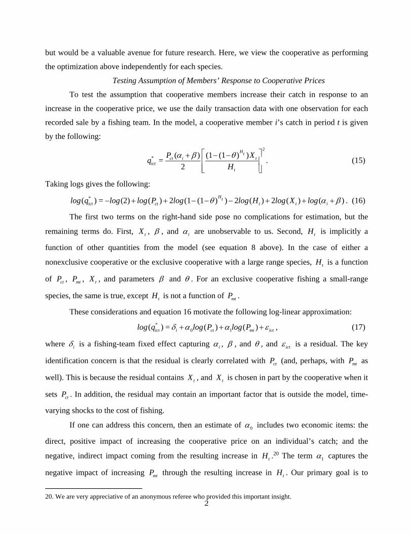
increase in the cooperative price, we use the daily transaction data with one observation for each

recorded sale by a fishing team. In the model, a cooperative member i’s catch in period t is given

by the following:

2

* ( ) (1 (1 ) )=

2

Htct i t

ictt

P Xq

H

. (15)

Taking logs gives the following:

*( ) = (2) ( ) 2 (1 (1 ) ) 2 ( ) 2 ( ) ( )Ht

ict ct t t ilog q log log P log log H log X log . (16)

The first two terms on the right-hand side pose no complications for estimation, but the

remaining terms do. First, tX , , and i are unobservable to us. Second, tH is implicitly a

function of other quantities from the model (see equation 8 above). In the case of either a

nonexclusive cooperative or the exclusive cooperative with a large range species, tH is a function

of ctP , mtP , tX , and parameters and . For an exclusive cooperative fishing a small-range

species, the same is true, except tH is not a function of mtP .

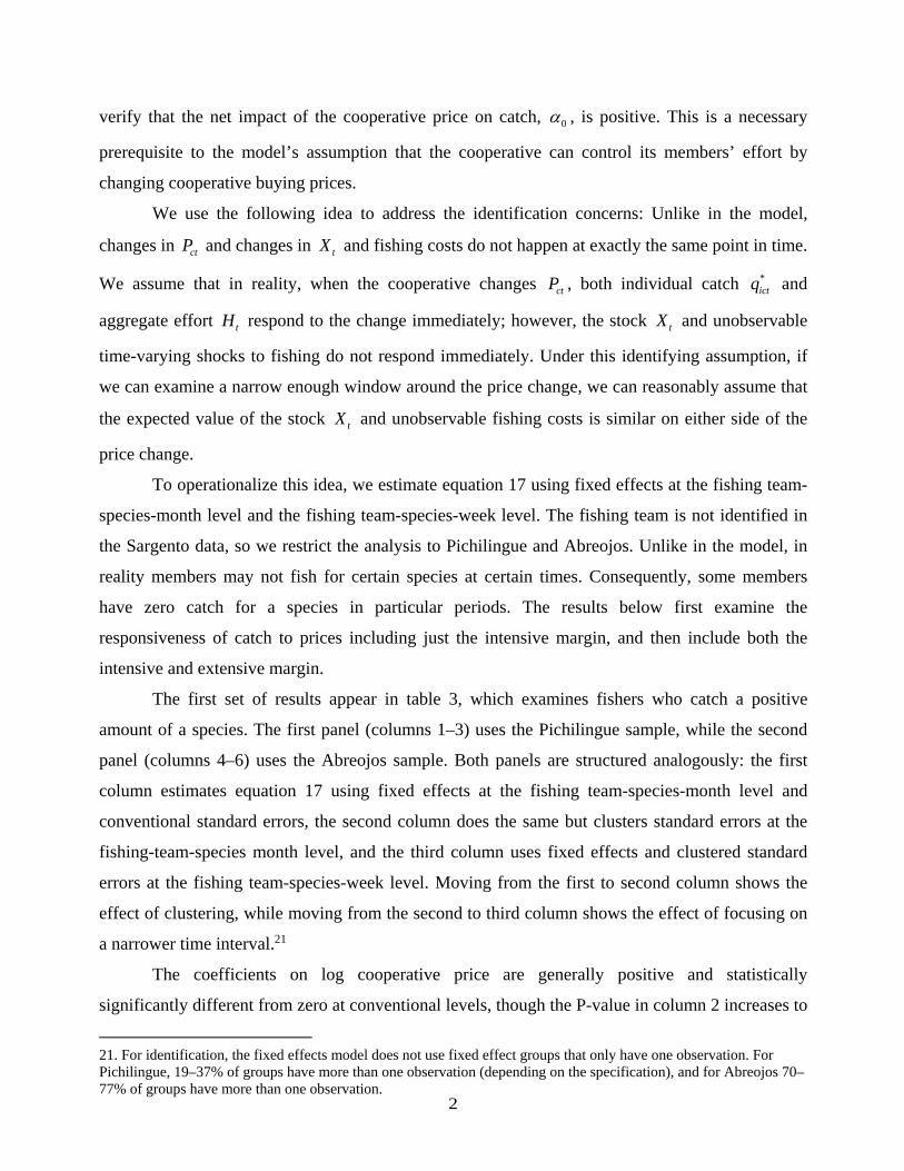
These considerations and equation 16 motivate the following log-linear approximation:

*0 1( ) = ( ) ( )ict i ct mt ictlog q log P log P , (17)

where i is a fishing-team fixed effect capturing i , , and , and ict is a residual. The key

identification concern is that the residual is clearly correlated with ctP (and, perhaps, with mtP as

well). This is because the residual contains tX , and tX is chosen in part by the cooperative when it

sets ctP . In addition, the residual may contain an important factor that is outside the model, time-

varying shocks to the cost of fishing.

If one can address this concern, then an estimate of 0 includes two economic items: the

direct, positive impact of increasing the cooperative price on an individual’s catch; and the

negative, indirect impact coming from the resulting increase in tH .20 The term 1 captures the

negative impact of increasing mtP through the resulting increase in tH . Our primary goal is to

                                                       20. We are very appreciative of an anonymous referee who provided this important insight.

2 

verify that the net impact of the cooperative price on catch, 0 , is positive. This is a necessary

prerequisite to the model’s assumption that the cooperative can control its members’ effort by

changing cooperative buying prices.

We use the following idea to address the identification concerns: Unlike in the model,

changes in ctP and changes in tX and fishing costs do not happen at exactly the same point in time.

We assume that in reality, when the cooperative changes ctP , both individual catch *ictq and

aggregate effort tH respond to the change immediately; however, the stock tX and unobservable

time-varying shocks to fishing do not respond immediately. Under this identifying assumption, if

we can examine a narrow enough window around the price change, we can reasonably assume that

the expected value of the stock tX and unobservable fishing costs is similar on either side of the

price change.

To operationalize this idea, we estimate equation 17 using fixed effects at the fishing team-

species-month level and the fishing team-species-week level. The fishing team is not identified in

the Sargento data, so we restrict the analysis to Pichilingue and Abreojos. Unlike in the model, in

reality members may not fish for certain species at certain times. Consequently, some members

have zero catch for a species in particular periods. The results below first examine the

responsiveness of catch to prices including just the intensive margin, and then include both the

intensive and extensive margin.

The first set of results appear in table 3, which examines fishers who catch a positive

amount of a species. The first panel (columns 1–3) uses the Pichilingue sample, while the second

panel (columns 4–6) uses the Abreojos sample. Both panels are structured analogously: the first

column estimates equation 17 using fixed effects at the fishing team-species-month level and

conventional standard errors, the second column does the same but clusters standard errors at the

fishing-team-species month level, and the third column uses fixed effects and clustered standard

errors at the fishing team-species-week level. Moving from the first to second column shows the

effect of clustering, while moving from the second to third column shows the effect of focusing on

a narrower time interval.21

The coefficients on log cooperative price are generally positive and statistically

significantly different from zero at conventional levels, though the P-value in column 2 increases to

                                                       21. For identification, the fixed effects model does not use fixed effect groups that only have one observation. For Pichilingue, 19–37% of groups have more than one observation (depending on the specification), and for Abreojos 70–77% of groups have more than one observation.

2 

0.103. The estimated elasticities of catch with respect to price range from 0.563 to 0.782, with

more stability for Abreojos across specifications. The coefficients on the market price are negative

in columns 1–2 as expected given the discussion above, but cannot be distinguished from zero in

any of the columns except one. The one exception is column 6, where we see an unexpected

positive sign. As noted in the context section above, Abreojos may have nonprice mechanisms with

which to induce members to fish; the significant positive coefficient is consistent with this, and

may suggest that our model captures only one mechanism through which cooperatives control

effort.22

The results that incorporate both the intensive and the extensive margin appear in table 4.

To incorporate both margins, we consider the exponentiated form of equation 17:

*0 1= ( ) ( )ict i ct mt ictq exp log P log P . (18)

Given that this equation is consistent with the conditional expectation function of the fixed effects

Poisson model, and given that a large fraction of observations are zeros, we estimate the model

using the Poisson quasi-maximum likelihood estimator with fixed effects at the fishing team-time-

species level.23 As discussed in Wooldridge (2010), ch. 18, and Burgess et al. (2012), the Poisson

model is a quasi-maximum likelihood estimator that yields consistent estimates as long as the

conditional expectation is correctly specified, regardless of the exact distribution of the underlying

error.

Table 4 is structured analogously to table 3. The coefficients can be interpreted as the

elasticity of the conditional expectation of catch with respect to price. The coefficient on log

cooperative price is positive and significant for every column except columns 2 and 3. This means

that the extensive margin effect appears stronger for Abreojos than Pichilingue. Except in one case,

the coefficient on market price is negative (and significant in columns 1 and 4).24

A complementary empirical approach, presented in the supplemental appendix, examines

changes in catch at the time of discrete events when there is a large and sustained change in

                                                       22. We also estimated these specifications without including the market price, even though this specification is only consistent with the theory in the case of small-range species at Abreojos. In these cases, when standard errors are clustered, the coefficient on log cooperative price is still positive and significant for Abreojos at the 1% level, ranging from 0.718 to 0.739. The Pichilingue coefficient falls to 0.375 (week-level regressions) and 0.205 (month-level regressions), with P-values of 0.141 and 0.335, respectively. Similar qualitative patterns hold when performing the same exercise for the specifications examining both the intensive and extensive margin in table 4. 23. The observations row in the table shows the number used for estimation; observations that do not show variation within group are not used. Among the observations used for estimation, 6871 (month specification) and 2480 (week specification) observations are zero for Pichilingue. The corresponding numbers for Abreojos are 36933 and 18296. 24. The exception is again column 6, the week specification for Abreojos, where the coefficient is positive but statistically indistinguishable from zero.

2 

cooperative prices for a species. Such events are difficult to pinpoint in the data. Still, the signs of

estimated coefficients are consistent with those above, though not always statistically significant.

Therefore, there is evidence that cooperative members respond to cooperative buying prices in the

way posited by the model.

Implication 1: Price Levels Across Cooperatives

Next, we test the model’s implications for how cooperatives choose buying prices. For this

portion of the analysis, we first aggregate the data to the cooperative-week-species level, taking the

sum of catch and the average log price across the week. The first implication of the model is if

market prices are constant and growth rates and 0X are the same across cooperatives, then on

average the exclusive cooperative will pay lower prices to its members than a nonexclusive

cooperative but will have higher catch.

To operationalize this comparison, note that in our forward-looking model without

uncertainty, the cooperative price in one period ctP will be a function of the exogenous variables

for every period, the initial stock 0X , and the cost parameter. Therefore, if we denote the exclusive

cooperative by E and the nonexclusive cooperative by N, we have for d=E,N:

0 0 0( ) = ( ),...., ( ), ,..., , ,ctd d m mT Tlog P g log P log P r r X , where the (.)dg are functions. In a more

general case, the cost term could also vary by time. A first-order Taylor series approximation of

the equations about the expected log market price ( )mlog P and the expected growth rate r yields:

0 0( ) = ( ( ) ( )) ... ( ( ) ( ))ctd d dp m m dpT mT mlog P g g log P log P g log P log P (19)

0 0( ) ... ( )dr drT T tdg r r g r r (20)

where dg is the function evaluated at ( )mlog P and r and contains 0X . The terms dptg and drtg

give the derivatives of dg with respect to ( )mtlog P and tr evaluated at the mean values of these

variables, respectively. Finally, ctd contains both approximation error and period-cooperative-

specific shocks to cost (if is allowed to vary by time). If tdD is a dummy variable equal to 1

when d=E and 0 otherwise, then the two equations can be combined:

=0

( ) = ( ) ( ) ( )( )T

ctd N E N td Nrt t td Ert Nrt tt

log P g g g D g r r D g g r r (21)

=0

( ( ) ( )) ( )( ( ) ( ))T

Npt mt m td Ept Npt mt mt

g log P log P D g g log P log P (22)

2 

( )tN td tE tND ò ò ò (23)

This motivates the following regression equation:

0 1( ) =ctd td tdlog P D u (24)

where:

=0

=0

= ( ( ) ( )) ( )( ( ) ( ))

( ) ( )( ) ( )

T

td Npt mt m td Ept Npt mt mt

T

Nrt t td Ert Nrt t tN td tE tNt

u g log P log P D g g log P log P

g r r D g g r r D

ò ò ò

Since both the exclusive and nonexclusive cooperative see the same market prices and growth rates

in any period, the expected value of tdu conditional on tdD is just ( ( ) | )tN td tE tN tdE D D ò ò ò .

Implication 1 of the model for prices is that 1( ) = < 0E Ng g . The above reasoning makes

clear what the threats to interpreting 1 in this way are. First, ( ( ) | )tN td tE tN tdE D D ò ò ò may not

be zero. To take an example, fishing costs may differ between exclusive and nonexclusive

cooperatives because of differences in species caught. Another possibility is that, since Abreojos

fishes some species that the other cooperatives do not, the two types of cooperatives systematically

see different market prices for output. To deal with this important issue, we use species-time fixed

effects. The fixed effects permit a comparison of cooperative prices within species-time period.

Second, 0X may not be the same across cooperatives within species.25 In this case, 1 reflects both

the mechanism stressed in the model simulations and the difference in initial stocks. We discuss

these identification concerns further below.

Finally, we can follow the same reasoning as above to develop an estimating equation for

catch:

0 1( ) =ctd td tdlog Q D v (25)

Implication 1 of the model for catch is that 1 > 0 . The identification concerns noted above are

applicable here as well.

We estimate equations 24 and 25 using fixed effects at the species-quarter, species-month,

and species-week levels.26 From the point of view of flexibly capturing time-varying unobservable

                                                       25. Coastal ocean productivity varies temporally, due to seasonal and longer-term drivers (e.g., ENSO). Ocean productivity also varies spatially between the Pacific and Gulf coasts of BCS (Lluch-Cota et al. 2010; Leslie et al. 2015), which could create differences in the productivity of fish populations. These effects are still not well understood. 26. The sample in both regressions uses only weeks in which at least one catch was recorded in the logbooks. Standard errors are clustered at the level of the fixed effect.

2 

costs, the species-week specification is most preferable. However, this uses a more limited subset

of data for identification. Reassuringly, the results are very similar with all three approaches.

The left panel of table 5 shows the results for log cooperative price, while the right panel

shows the results for log weekly catch. Within species and time period, prices are more than one

log point lower in Abreojos than the other cooperatives (columns 1–3). The magnitude is quite

similar across the columns. This suggests that within a species-quarter combination, omitted

determinants of log cooperative prices that vary by week or month are not strongly correlated with

the Abreojos dummy. The coefficient on the Abreojos dummy in the catch specifications also has

the expected sign (columns 4–6). Within species and time period, log catch is substantially higher

in Abreojos than the other cooperatives.

Above, we raised a number of endogeneity concerns. The stability of the coefficient

estimates across the columns in table 5 may alleviate some of these concerns. Moreover, some of

these concerns are less problematic when one considers both the price and catch results

simultaneously. For instance, the catch results could be driven by the fact that initial stocks of all

species are exogenously higher on the Pacific side of B.C.S. (near Abreojos) compared to the Gulf

of California side (near Pichilingue and Sargento). But this by itself would not explain the negative

coefficient in the price regressions. Similarly, differences in the number of members across

Abreojos and the other cooperatives could explain the differences in catch but not necessarily the

differences in prices. If market prices are systematically lower for Abreojos than for the other

cooperatives even within a species—since Abreojos sells in part to different markets—this could

explain the price results, but not the catch results.

Nevertheless, there is still a class of relevant endogeneity concerns: If the area around

Abreojos is more productive ecologically, fishing costs could simply be lower for Abreojos; this

could lead to lower cooperative prices and higher catch totals. The next subsection shows that,

while this effect may be at work, it does not fully capture the patterns in the data.

Implication 2: Role of Species Scale in Price Gaps

Next, we examine the second implication of the model: The gap in prices and catch

between cooperatives with exclusive property rights and cooperatives without exclusive rights will

be smaller in magnitude for species that have a larger scale of movement. The development of an

empirical specification to test implication 2 is similar to the case of implication 1. Instead of

allowing the functions g(.) to differ based only on whether the cooperative is exclusive or not, there

are now four possible combinations (d,x), d=E,N, x=L,S: exclusive, large-scale (EL); exclusive,

3 

small-scale (ES); nonexclusive, large scale (NL); and nonexclusive, small scale (NS). If xL is a

dummy variable that is 1 for large scale species and 0 otherwise, the Taylor series expansion about

the scale-specific expected growth rates and expected log prices yields:

( ) = ( ) ( ) ( ) ( )ctdx NS ES NS td NL NS x EL NL ES NS td x tdxlog P g g g D g g L g g g g D L u (26)

where tdxu is a function of prices, growth rates, and tdxò analogous to the one in the previous

subsection, except now including the scale-specific expected growth rates and expected log prices,

tdD , xL , and the interaction of the two.

This motivates the following regression equation:

0 1 2 3( ) =ctdx td x td x tdxlog P D L D L u (27)

Assuming again that the two types of cooperatives see the same market prices and growth rate for a

given species, the expectation of tdxu conditional on tdD and xL simplifies to the following:

( ) ( ) ( ) ( ) | ,NS ES NS td NL NS x EL NL ES NS td x td xE D L D L D L ò ò ò ò ò ò ò ò ò

Implication 2 of the model is that, with all else held equal, 3 > 0 . As above, there are two types of

threats to interpreting 3 as reflecting the model’s mechanisms. First, the expectation in the

expression just above may not be zero. This could happen, for instance, if the difference in fishing

costs between the exclusive and nonexclusive cooperative varies by the scale of the species. Since

one source of this issue is differences in the type of species caught, we again use species-time fixed

effects. The second type of identification concern is that the difference in 0X between the

exclusive cooperative and the nonexclusive cooperatives could vary depending on scale. For both

identification concerns, the crucial issue is whether the difference between the exclusive and

nonexclusive cooperatives varies by scale. For example, simply having a difference in fishing costs

between exclusive and nonexclusive cooperatives that is invariant to species scale biases the

estimate of 1 but not the estimate of 3 . In this sense, the test of implication 2 is more robust than

that of implication 1 and is analogous to a differences-in-differences approach.

Analogous reasoning leads to an estimating equation for catch:

0 1 2 3( ) =Ctdx td tdx td tdx tdxlog Q D L D L v (28)

Implication 2 of the model for catch is that 3 < 0 .

As in the previous subsection, we estimate equation 27 and 28 using fixed effects first at the

3 

species-quarter level, then the species-month level, and finally at the species-week level.27 The left

panel of table 6 shows the regressions for log price, and the right panel shows the regressions for

log weekly catch.

There is again stability in the coefficients across the various specifications. As expected, the

coefficient on the Abreojos dummy—reflecting the price gap for small scale species—is always

negative and significant (columns 1–3). More interesting is the coefficient on the interaction

between the Abreojos dummy and the large scale dummy. As predicted by the theory, this

coefficient is positive and statistically different from zero. The magnitude suggests that the gap in

prices between Abreojos and the other cooperatives is reduced by 15–17% when considering

species that are more highly mobile (columns 1–3). The results for catch also confirm the theory:

While weekly catch is higher in Abreojos than in the other cooperatives, this difference is cut in

half for large scale species (columns 4–6).

This is consistent with the idea that Abreojos exerts less control of effort over large scale

species relative to small scale species. These results also narrow the class of alternative

explanations that can capture the data. For example, if lower fishing costs near Abreojos than near

the other cooperatives are driving the results, then it must be the case that the cost difference is

lower for large scale species than for small scale species.

Implication 3: Changes in Growth Rates

The third implication of the model is that the difference in prices between a nonexclusive

cooperative and an exclusive cooperative will rise when population growth rates fall, and fall when

population growth rates rise. Essentially, the exclusive cooperative acts more aggressively to limit

effort when growth rates are projected to be low.

To develop an estimating equation to test the prediction, first consider the cooperative’s

maximization problem in equation 11 above. Let t be the Lagrange multiplier on the constraint

for the 1tX stock equation, and note that tH is an implicitly defined function of ( , , )t ct mtX P P and

* is an implicitly defined function of ( , )ct mtP P . The first-order condition with respect to ctP can

then be written in general as 1( , , , , ; , , ) = 0ct mt t t tG P P X r , where G(.) is a function and

( , , ) give the discount rate, costs of fishing, and the extraction rate from fishing effort. This

means that ( )ctdlog P for cooperative of type d=E,N can be written in general as:

                                                       27. The sample in both regressions uses only weeks in which at least one catch was recorded in the logbooks. Standard errors are clustered at the level of the fixed effect.

3 

1( ) = ( ( ), , , , , , )ctd d mt td t tdlog P g log P X r , where this could be further generalized to allow for

time-varying and cooperative-varying costs by substituting td for .

We begin again with a Taylor series approximation of this function about the expected

values of all arguments:

1( ) = ( ( ) ( )) ( )ctd d dp mt m dr tlog P g g log P log P g r r (29)

( ) ( )dx td d d td d tdg X X g ò (30)

where dg is the function evaluated at the expected values and all other bars indicate expected

values. The additional subscripts on g indicate derivatives with respect to a variable, evaluated at

the expected values. Here, td is approximation error and, if is allowed to vary by time and

cooperative type, period/cooperative-specific shocks to fishing costs (similarly, td could reflect

shocks to other parameters). Both cooperatives see the same values of mtP and 1tr .

Let tdD equal 1 when d=E and 0 otherwise. Then, similarly to above, we have:

( ) = ( ) ( ( ))( ( ) ( ))ctd N td E N Np td Ep Np mt mlog P g D g g g D g g log P log P (31)

1( ( ))( ) ( ( ))( )Nr td Er Nr t N td E N td dg D g g r r g D g g (32)

( ( ))( )Nx td Ex Nx td d tdg D g g X X ò (33)

Implication 3 of the model concerns the difference in the correlation between ( )ctlog P and

1( )tlog r across exclusive and nonexclusive cooperatives, holding market prices, fishing costs, and

initial stock constant. This derivation makes several challenges clear. First, there are items in tdò

that are potentially correlated with the observable variables. Time-varying costs, for example, may

be related to market prices if these prices are locally determined. Another possibility is that the

differential effects of species scale across cooperatives, as shown above. Second, differences in two

key unobservables—stock tdX and Lagrange multiplier td —reflect differences in market prices,

fishing costs, and initial stock. Third, and finally, direct data on growth rates are not available.

Instead, we use ONI as a proxy variable. Since ONI increases growth rates for some species and

reduces growth rates for others, as discussed above, we must account for species-specific responses

to ONI in the specification. Our classification of these responses will introduce measurement error.

To deal with these issues, we estimate the following specification in the empirical analysis

using data on the species-week level for each cooperative:

3 

0 1 2 3 4 5( ) = ( ) ( )ctdx td td x mtx td mtx tlog P D D L log P D log P ONI (34)

6 7 8 9td t td x x t td x t xp tdxD ONI D R R ONI D R ONI u (35)

where x is the species subscript and xL is the dummy for large scale as in the discussion of

implication 2. tONI is our ONI measure (varying at the month level). Including td tD ONI allows

for baseline differences across geographic areas in response to ONI for species whose recruits have

no known response to ONI; the adults of these species may still respond to ONI. xR is a variable

equal to -1 if ONI has negative effects on recruitment of species x, equal to 1 if ONI has positive

effects and 0 if there is no established consensus. Finally, xp is a species-time period-specific

fixed effect, where a time period is a month in the preferred specifications below.

Implication 3 of the model is that 9 > 0 : the 9 coefficient indicates the difference across

cooperatives in responding to other species’ positive or negative responses to ONI. Our identifying

assumption is that, after controlling for the other observables in equation 34, no factor in tdxu leads

to differential effects of ONI across cooperatives. The remaining threats to identification must take

a very particular form. For instance, tdxX and tdx are omitted from the estimating equation. The

cooperative dummy tdD and the species-time period-specific fixed effect xp capture the

components of these unobservables that are additively separable between these items, so the

remaining problem comes from components that are cooperative-species-specific. An example that

could generate the patterns we see in the data is that the initial stock 0X might be higher near

Abreojos only for those species that respond positively to ONI. While we cannot prove an

explanation like this is not at work, below we show that our basic results are robust to a number of

changes in the specification.

Table 7 shows the results from estimating versions of equation 34. The first column shows

the base specification, using fixed effects at the species-month level. The first two rows show the

results for the Abreojos main effect and the interaction with the large scale species dummy. These

coefficients have the expected signs, given the discussion of implications 1 and 2 above. The third

and fourth rows show how the market prices are correlated with cooperative prices for each

cooperative. The next two rows contain the interactions of Abreojos with ONI and the Recruit

Effect ( xR from above). Finally, the last row contains the estimate of 9 . This shows that when

growth rates change due to ONI, the price difference between Abreojos and other cooperatives

3 

moves in the predicted direction. The coefficient 9 implies a 16% price change in response to a

one standard deviation change in ONI.

A serious concern with this result is that market prices may be correlated with fishing costs.

Above, we saw that our three cooperatives are not dominant players in the La Paz market, so they

are unlikely to be able to affect market prices directly with their own actions. Moreover, for at least

some species, market prices in La Paz seem to be related to prices in a market that should be

relatively unaffected by supply-side issues in B.C.S. Still, if at least some market prices are locally

determined, a large positive shock to fishing costs of every player in B.C.S. may cause a large

positive shock to market prices as well. Our species-month fixed effect deals with this issue in part;

but it could still be the case that a weekly shock in costs relative to the monthly mean is associated

with a weekly shock to market prices. This endogeneity could then cause a bias in the coefficient of

interest that would be difficult to sign.

We deal with this issue in two ways. First, we instrument for market prices and the

interaction of market prices with the Abreojos dummy. As our instruments we use a lag of market

prices and the interaction of the lag with the Abreojos dummy. Column 2 uses the one period lag,

while column 3 uses the two period lag. The estimates of 9 are quite similar to the estimate in

column 1. Nevertheless, this solution has several problems. If weekly shocks to costs from the

monthly mean are correlated across time, then the period t shock in the residual could be correlated

with the instruments. Even if the exclusion restriction is satisfied, these are not strong instruments.

The Kleibergen-Paap LM statistic for column 2 is large enough that we can reject the null

hypothesis of underidentification at the 10% level, but we fail to reject with the corresponding

Wald statistic. In column 3, we fail to reject with both statistics.

Therefore, we also estimate the standard fixed effects model without incorporating the

market prices. While this deviates from the theoretically inspired specification, it is still useful: If

the remaining coefficients change dramatically, this suggests that the endogeneity of market prices

could cause large biases. The results appear in column 4. Reassuringly, 9 is still positive,

statistically different from zero, and of similar magnitude.

Finally, we test the sensitivity of the results to the level of the fixed effect. With a less

flexible set of fixed effects (species-quarter), 9 falls in size and becomes statistically

indistinguishable from zero (column 5). However, with species-week fixed effects, 9 is again

3 

positive and significant, and the magnitude is closely comparable to the baseline

specification (column 6).28

Alternative Explanations

There are historical and geographic differences between Abreojos and the other two

cooperatives. An important concern is that the empirical patterns above reflect these other

differences, rather than the difference in property rights. The tests of implications 2 and 3 help

greatly in this regard. The empirical specifications testing these implications are essentially

difference-in-difference models: while the Abreojos dummy may be endogenous to price and catch

levels, the estimated coefficients on the key interaction terms are unbiased as long as the source of

endogeneity does not differ by species scale or by species-specific responses to environmental

oscillations.

One specific concern, for example, is that Abreojos’s distance from La Paz leads to higher

costs for selling catch, and this cost is taken out of payments to cooperative members. This

explains the negative coefficient on the Abreojos dummy in the buying price regressions above.

However, this explanation is problematic. First, the cost difference is unlikely to be large: Abreojos

has streamlined methods of transporting, processing, and marketing catch through its operations in

La Paz and Enseñada, as well as FEDECOOP’s exports. Second, the explanation cannot capture the

fact that the price gap between Abreojos and Pichilingue/Sargento is smaller for large-scale

species.

One could supplement the above alternative explanation with the idea that, relative to the

other cooperatives, Abreojos faces a smaller disadvantage in marketing catch for its exports to the

United States and elsewhere. If large-scale species are more often exported, this could explain the

fact that the price gap between Abreojos and Pichilingue/Sargento is smaller for large-scale

species. However, this explanation is also problematic. Of the species for which we have market

price data, Abreojos’s most salient exports are lobster and sea bass, and both species are small-

scale.29 Moreover, this alternative explanation cannot explain our third finding, that the price gap is

responsive to ONI and the specific effect of ONI (positive or negative) on a particular species.

The geographic differences between Abreojos and the other cooperatives suggest there may                                                        28. Throughout, we have used the sample for which we have nonmissing cooperative prices and nonmissing market

prices. In specifications not shown here, we show that 9 continues to be positive and significant with species-week

fixed effects when this sample is broadened to all observations without nonmissing cooperative prices. However, 9 is

smaller and insignificant with this sample when using species-month fixed effects. 29. By “salient,” we mean products advertised on the FEDECOOP website: http://www.fedecoop.com.mx/. Abalone, another small-scale species, is a key export of Abreojos, but we do not have market price data for this species.

3 

be differential stock endowments across the two areas. This could explain our results for

differential catch, but such an alternative explanation would have to take a particular form to

capture both of our empirical results: specifically, the stock advantage of the Pacific side would

have to be relatively larger for small scale species than for large scale species. Existing work

suggests the presence of differences in ocean productivity in the Pacific versus Gulf sides of the

Baja Peninsula; unfortunately, however, not much is known (as far as we are aware) about how

these differences manifest differentially across small scale and large scale species. Therefore, this

alternative explanation for our catch results may be plausible, and we do not have evidence to

support or refute it at this time. Nevertheless, we believe our model is the most plausible

explanation that captures all of the empirical patterns we have seen for price and catch in one

unified framework.

V CONCLUSION

In this paper, we set out to understand how cooperatives use property rights to control

fishing effort, and how this use is shaped by key characteristics of the targeted fish populations:

scale of individual movement and responses to large environmental fluctuations. Using rich

logbook data from three cooperatives, including one that enjoys strong property rights, we find

support for the implications of our theoretical model. The magnitude of the differences between the

cooperative with property rights and the ones without rights—as well as the shrinking of these

differences when resources have a large scale or when growth rates are high—are economically

significant.

These results highlight the value of linking theory with empirical analysis in order to

examine the reciprocal interactions between natural resources and resource users. Our approach

focuses on the economic mechanisms underlying these interactions and thereby complements more

descriptive, existing analyses of fishery outcomes. Our results are also relevant beyond fisheries, as

they illustrate how the decisions of resource users embedded in local institutions are mediated by

characteristics of the resource and external dynamic factors. However, given that our logbook data

are restricted to only three cooperatives, our conclusions are necessarily provisional. We hope that

our analysis points the way to future investigation with more representative data.

More generally, integration of the connections between resources and resource users may

well increase the effectiveness of state policies in coastal areas, whether focused on environmental

stewardship, economic development, or both. Indeed, CONAPESCA’s recently developed National

Program of Inspection and Vigilance (Programa Nacional de Inspección y Vigilancia)

3 

demonstrates the government’s interest in involving the leaders of local user groups in fisheries

management; the program calls for the formation of state committees that include representatives

of national, state, and local governments, as well as representatives of fisher groups.30 Our results

suggest that even greater devolution of authority to local users—by granting property rights—could

be a viable management strategy in the right circumstances. By recognizing the influence that local

institutions like Mexico’s fishing cooperatives may have on both ecological and economic

outcomes, policymakers will be better able to craft proactive, ecosystem-based policies that sustain

both marine resources and the human communities that rely on them.

References

Aburto-Oropeza, O., E. Sala, G. Paredes, A. Mendoza, and E. Ballesteros. 2007. “Predictability of Feef Fish Recruitment in a Highly Variable Nursery Habitat.” Ecology 88 (9), 2220–28.

Acosta, C. A. 1999. “Benthic Dispersal of Caribbean Spiny Lobsters among Insular Habitats: Implications for the Conservation of Exploited Marine Species.” Conservation Biology 13 (3), 603–612.

Allison, E. H., and F. Ellis. 2001. “The Livelihoods Approach and Management of Small-Scale Fisheries.” Marine Policy 25 (5), 377–88.

Basurto, X., A. Bennett, A. Weaver, S. Rodriguez-Van Dyck, and J.-S. Aceves-Bueno. 2013. “Cooperative and Noncooperative Strategies for Small-Scale Fisheries’ Self-Governance in the Globalization Era: Implications for Conservation.” Ecol. Soc. 18 (38).

Basurto, X., and E. Coleman. 2010. “Institutional and Ecological Interplay for Successful Self-Governance of Community-Based Fisheries.” Ecological Economics 69 (5), 1094–103.

Branch, T. A., O. P. Jensen, D. Ricard, Y. Ye, and R. Hilborn. 2011. “Contrasting Global Trends in Marine Fishery Status Obtained from Catches and from Stock Assessments.” Conservation Biology 25 (4), 777–86.

Burgess, R., M. Hansen, B. A. Olken, P. Potapov, and S. Sieber. 2012. “The Political Economy of Deforestation in the Tropics.” Quarterly Journal of Economics 1707–54.

Calderon-Aguilera, L., S. Marinone, and E. Aragón-Noriega. 2003. “Influence of Oceanographic Processes on the Early Life Stages of the Blue Shrimp (Litopenaeus stylirostris) in the Upper Gulf of California.” Journal of Marine Systems 39 (1), 117–28.

Carson, R. T., C. Granger, J. Jackson, and W. Schlenker. 2009. “Fisheries Management under Cyclical Population Dynamics.” Environmental and Resource Economics 42 (3), 379–410.

Clark, C. W. 1990. Mathematical Bioeconomics: Optimal Management of Renewable Resources, Hoboken, NJ: John Wiley and Sons Inc.

Costello, C., S. D. Gaines, and J. Lynham. 2008. “Can Catch Shares Prevent Fisheries Collapse?” Science 321 (5896), 1678–81.

Costello, C. and D. T. Kaffine. 2010), “Marine protected areas in spatial property-rights fisheries.” Australian Journal of Agricultural and Resource Economics 54 (3), 321–41.

                                                       30. For details, see http://www.conapesca.sagarpa.gob.mx/wb/cona/programa_nacional_de_inspeccion_vigilancia_

3 

Costello, C., S. Polasky, and A. Solow. 2001. “Renewable Resource Management with Environmental Prediction.” Canadian Journal of Economics/Revue Canadienne d’ Économique 34 (1), 196–211.

Cota-Nieto, J. 2010. Descripción história y reciente de las pesquerías artesanales de punta abreojos B.C.S., México. periodo 2000–2007., Thesis, Universidad Autónoma de Baja California Sur.

Deacon, R. T. 2012. “Managing Fisheries by Assigning Rights to Harvester Cooperatives.” Review of Environmental Economics and Policy 6 (2), 258–77.

Deacon, R. T., D. P. Parker, and C. Costello. 2008. “Improving Efficiency by Assigning Harvest Rights to Fishery Cooperatives: Evidence from the Chignik Salmon Co-op.” Arizona Law Review 50 (2).

———. 2013. “Reforming Fisheries: Lessons from a Self-Selected Cooperative.” Journal of Law and Economics 56 (1).

DeWalt, B. R. 2001. “Community Forestry and Shrimp Aquaculture in Mexico: Social and Environmental Issues.” presentado en la Latin American Studies Association, Washington DC 6.

Dong, D., B. W. Gould, and H. M. Kaiser. 2004. “Food Demand in Mexico: An Application of the Amemiya-Tobin Approach to the Estimation of a Censored Food System.” American Journal of Agricultural Economics 86 (4), 1094–107.

Eberhardt, L. 1977. “Relationship between Two Stock-Recruitment Curves.” Journal of the Fisheries Research Board of Canada 34 (3), 425–28.

Edmonds, E. V. 2002. “Government-Initiated Community Resource Management and Local Resource Extraction from Nepal’s Forests.” Journal of Development Economics 68 (1), 89–115.

Foster, A. D. and M. R. Rosenzweig. 2003. Agricultural Development, Industrialization and Rural Inequality, Technical report, Cambridge, Massachusetts: Harvard University.

Gordon, H. S. 1954. “The Economic Theory of a Common-Property Resource: The Fishery.” The Journal of Political Economy 62(2), 124–142.

Gutiérrez, N. L., R. Hilborn, and O. Defeo. 2011. “Leadership, Social Capital and Incentives Promote Successful Fisheries.” Nature 470 (7334), 386–89.

Hilborn, R., J. K. Parrish, and K. Litle. 2005. “Fishing Rights or Fishing Wrongs?” Reviews in Fish Biology and Fisheries 15 (3), 191–99.

Ibarra, A. A. 1996. “Fisheries Trade under NAFTA and a Comparison with the EU,” Technical report, Instituto Nacional De La Pesca, Mexico City.

Ibarra, A. A., C. Reid, and A. Thorpe. 1998. Neo-Liberalism and the Latin “Blue Revolution” Fisheries Development in Chile, Mexico and Peru, University of Portsmouth, Centre for the Economics and Management of Aquatic Resources.

———. 2000. “The Political Economy of Marine Fisheries Development in Peru, Chile and Mexico.” Journal of Latin American Studies 32 (02), 503–27.

3 

Leslie, H. M., X. Basurto, M. Nenadovic, L. Sievanen, K. C. Cavanaugh, J. J. Cota-Nieto, B. E. Erisman, et al. 2015. “Operationalizing the Social-Ecological Systems Framework to Assess Sustainability.” PNAS 112 (19), 5979–84.

Lester, S. E., B. S. Halpern, K. Grorud-Colvert, J. Lubchenco, B. I. Ruttenberg, S. D. Gaines, S. Airamé, and R. R. Warner. 2009. “Biological Effects within No-Take Marine Reserves: A Global Synthesis.” Marine Ecology Progress Series 384, 33–46.

Lluch-Cota, S., A. Pares-Sierra, V. Magana-Rueda, F. Arreguin-Sanchez, G. Bazzino, H. Herrera-Cervantes, and D. Lluch-Belda. 2010. “Changing Climate in the Gulf of California.” Progress In Oceanography 87, 114–26.

Mann, K., and J. Lazier. 2005. Dynamics of Marine Ecosystems: Biological-Physical Interactions in the Oceans, Wiley-Blackwell.

McCay, B. J., F. Micheli, G. Ponce-Díaz, G. Murray, G. Shester, S. Ramirez-Sanchez, and W. Weisman. 2014. “Cooperatives, Concessions, and Co-management on the Pacific Coast of Mexico.” Marine Policy 44, 49–59.

McGuire, T. R. 1983. “The Political Economy of Shrimping in the Gulf of California.” Human Organization 42 (2), 132–45.

OECD 2006. Agricultural and Fisheries Policies in Mexico: Recent Achievements, Continuing the Reform Agenda, Organisation for Economic Cooperation and Development Publishing.

Ostrom, E. 1990. Governing the Commons: The Evolution of Institutions for Collective Action, Cambridge University Press: Cambridge (UK).

Ovando, D. A., R. T. Deacon, S. E. Lester, C. Costello, T. Van Leuvan, K. McIlwain, C. Kent Strauss, et al. 2013. “Conservation Incentives and Collective Choices in Cooperative Fisheries.” Marine Policy 37, 132–40.

Parma, A. M., and R. B. Deriso. 1990. “Experimental Harvesting of Cyclic Stocks in the Face of Alternative Recruitment Hypotheses.” Canadian Journal of Fisheries and Aquatic Sciences 47 (3), 595–610.

Pauly, D. 1997. Small-Scale Fisheries in the Tropics: Marginality, Marginalization, and Some Implications for Fisheries Management, in E. Pikitch, D. Hupert and M. Sissenwine, eds, “Global trends: Fisheries Management.” American Fisheries Society Symposium 20: Bethesda, Maryland, 40–49.

Petterson, J. S. 1980. “Fishing Cooperatives and Political Power: A Mexican Example.” Anthropological Quarterly 64–74.

Polis, G., M. Rose, F. Sanchez Pinero, P. Stapp, and W. Anderson,. 2002. “Island Food Webs,” in A New Island Biogeography of the Sea of Cortes. New York: Oxford UP, 280–362.

Reddy, S. M., A. Wentz, O. Aburto-Oropeza, M. Maxey, S. Nagavarapu, and H. M. Leslie. 2013. “Evidence of Market-Driven Size-Selective Fishing and the Mediating Effects of Biological and Institutional Factors.” Ecological Applications 23 (4), 726–41.

Reed, W. J. 1975. “A Stochastic Model for the Economic Management of a Renewable Animal Resource.” Mathematical Biosciences 22, 313–37.

Sáenz-Arroyo, A., C. M. Roberts, J. Torre, M. Cariño-Olvera, and R. R. Enríquez-Andrade. 2005. “Rapidly Shifting Environmental Baselines among Fishers of the Gulf of California.” Proceedings of the Royal Society B: Biological Sciences 272 (1575), 1957–62.

4 

Sala, E., O. Aburto-Oropeza, M. Reza, G. Paredes, and L. G. López-Lemus. 2004. “Fishing Down Coastal Food Webs in the Gulf of California.” Fisheries 29 (3), 19–25.

Sanchez, A., J. J. C. Nieto, I. M. Osorio, B. Erisman, M. Moreno-Baez, and O. Aburto-Oropeza. 2015. Caracterizacion de las cadenas productivas pesqueras – baja california sur, mexico (primera fase la paz). Database, Centro para la Biodiversidad Marina y la Conservacion (CMBC) and Scripps Institution of Oceanography.

Schaefer, K. M., D. W. Fuller, and B. A. Block. 2007. “Movements, Behavior, and Habitat Utilization of Yellowfin Tuna (Thunnus albacares) in the Northeastern Pacific Ocean, Ascertained through Archival Tag Data.” Marine Biology 152 (3), 503–25.

Scott, A. 1956. “The Fishery: The Objectives of Sole Ownership.” The Journal of Political Economy 63 (2), 116–24.

SEPESCA 1992. Legal Framework for Fisheries 1992, Technical report, Secretaria de Pesca, Mexico City.

Sievanen, L. 2014. “How do small-scale fishers adapt to environmental variability? lessons from Baja California Sur, Mexico.” Maritime Studies . 13:9:doi:10.1186/s40152-40014-40009-40152.

Velarde, E., E. Ezcurra, M. A. Cisneros-Mata, and M. F. Lavín, M. F. 2004. “Seabird Ecology, El Niño Anomalies, and Prediction of Sardine Fisheries in the Gulf of California.” Ecological Applications 14 (2), 607–15.

Villa, A. 1996. “A Review of Recent Changes in Mexico’s Fishing Policy,” thesis, College of Marine Studies at the University of Delaware.

White, C. and C. Costello. 2011), “Matching Spatial Property Rights Fisheries with Scales of Fish Dispersal.” Ecological Applications 21, 350–62.

Wilen, J. E., J. Cancino, and H. Uchida. 2012. “The Economics of Territorial Use Rights fisheries, or TURFs.” Review of Environmental Economics and Policy (62), 237–57.

Wooldridge, J. 2010. Econometric Analysis of Cross Section and Panel Data, Second Edition, Cambridge, MA: The MIT Press.

Young, E. 2001. “State Intervention and Abuse of the Commons: Fisheries Development in Baja California Sur, Mexico.” Annals of the Association of American Geographers 91 (2), 283–306.

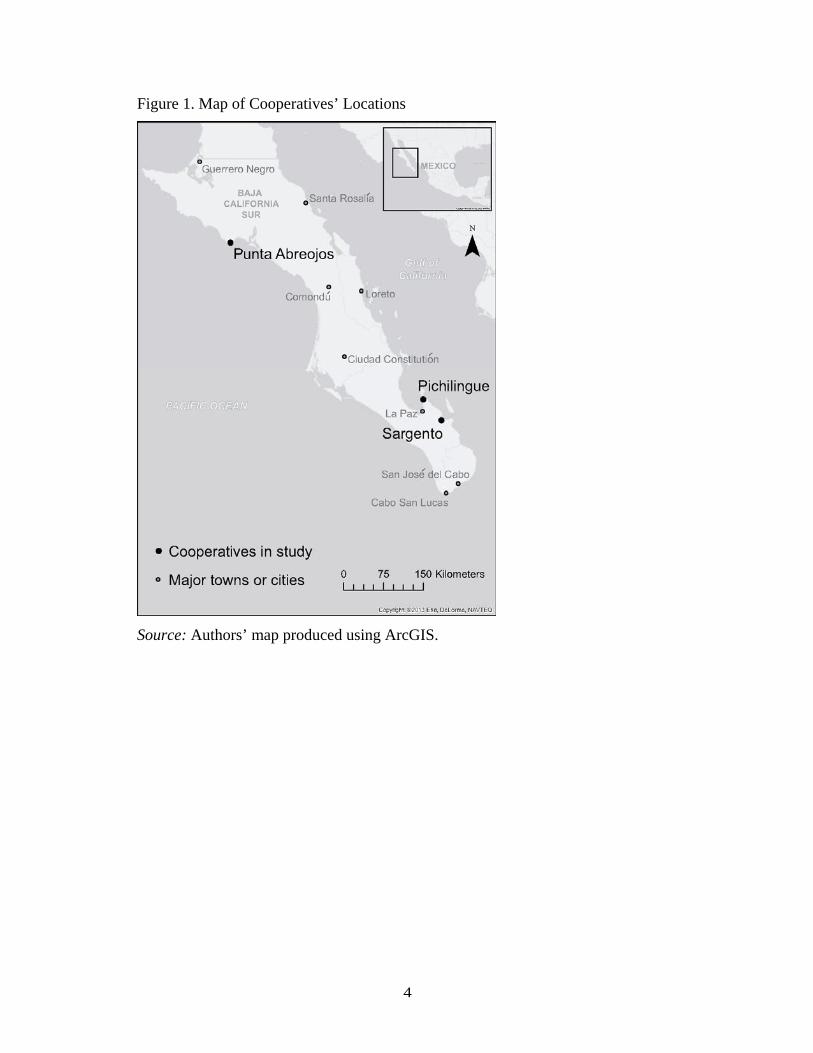
4 

Figure 1. Map of Cooperatives’ Locations

Source: Authors’ map produced using ArcGIS.

4 

Figure 2. Frequency Distribution of ONI Effect on Recruits

Source: Authors’ analysis based on cooperative database described in the main text.

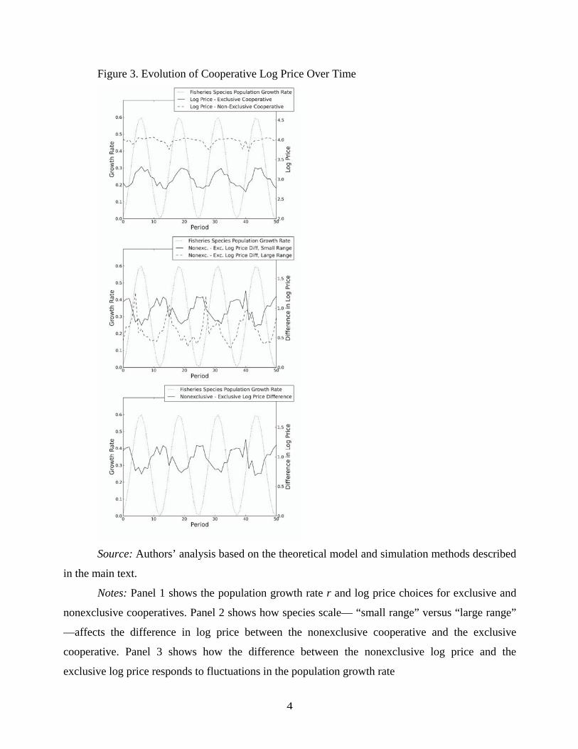
4 

Figure 3. Evolution of Cooperative Log Price Over Time

Source: Authors’ analysis based on the theoretical model and simulation methods described

in the main text.

Notes: Panel 1 shows the population growth rate r and log price choices for exclusive and

nonexclusive cooperatives. Panel 2 shows how species scale— “small range” versus “large range”

—affects the difference in log price between the nonexclusive cooperative and the exclusive

cooperative. Panel 3 shows how the difference between the nonexclusive log price and the

exclusive log price responds to fluctuations in the population growth rate

4 

Figure 4. Evolution of Cooperative Log Catch Over Time

Source: Authors’ analysis based on the theoretical model and simulation methods described

in the main text.

Notes: Panel 1 shows the population growth rate r and log catch for exclusive and

nonexclusive cooperatives. Panel 2 shows how species scale—“small range” versus “large

range”—affects the difference in log catch between the nonexclusive cooperative and the exclusive

cooperative. Panel 3 shows how the difference between the nonexclusive log catch and the

exclusive log catch responds to fluctuations in the population growth rate.

4 

Table 1. Summary Statistics

All cooperatives

Variable N Mean Std. dev. Min. Max.

Log catch 5015 4.436 2.062 -1.609 11.258

Log coop price 4310 2.848 1.002 0.729 6.034

Log mkt price 3325 3.365 0.832 0.729 6.061

Large scale

(0/1)

5014 0.373 0.484 0.000 1.000

ONI 5015 -0.181 0.776 -1.400 1.800

Recruit effect (-

1/0/1)

5014 0.039 0.527 -1.000 1.000

ONI X recruit

effect

5014 -0.018 0.426 -1.800 1.800

Pichilingue and Sargento

Variable N Mean Std. dev. Min. Max.

Log catch 3091 4.170 1.646 0.000 8.790

Log coop price 3005 3.228 0.708 1.640 6.034

Log mkt price 2145 3.476 0.714 0.950 6.054

Large scale

(0/1)

3090 0.312 0.463 0.000 1.000

ONI 3091 -0.197 0.754 -1.400 1.800

Recruit effect (-

1/0/1)

3090 0.067 0.608 -1.000 1.000

ONI X recruit

effect

3090 -0.023 0.475 -1.800 1.800

Abreojos

Variable N Mean Std. Dev. Min. Max.

Log catch 1924 4.864 2.537 -1.609 11.258

Log coop price 1305 1.975 1.032 0.729 5.907

Log mkt price 1180 3.163 0.982 0.729 6.061

4 

Large scale

(0/1)

1924 0.470 0.499 0.000 1.000

ONI 1924 -0.155 0.811 -1.400 1.800

Recruit effect (-

1/0/1)

1924 -0.005 0.355 -1.000 1.000

ONI X recruit

effect

1924 -0.010 0.331 -1.800 1.800

Table 2. Relationship Between La Paz and La Nueva Viga (LNV) Prices

Common name of species (in Spanish)

Variable Almeja Calamar Camaron Cazon Jurel Lisa Mojarra Ostion Pulpo

LNV

log price

0.313** 0.606*** -0.146 0.102*** -

0.231***

0.145*** 0.124 -

0.207***

0.123***

(0.133) (0.026) (0.133) (0.020) (0.012) (0.027) (0.085) (0.025) (0.040)

Constant -0.182 0.484*** 5.769*** 2.777*** 3.691*** 1.971*** 1.851*** 5.939*** 3.637***

(0.449) (0.069) (0.655) (0.073) (0.035) (0.076) (0.292) (0.113) (0.172)

Obs 42 80 35 1528 1903 110 152 113 103

R2 0.121 0.877 0.035 0.016 0.170 0.207 0.014 0.373 0.085

Note: All specifications use OLS with the log of the price in La Paz as the dependent

variable.

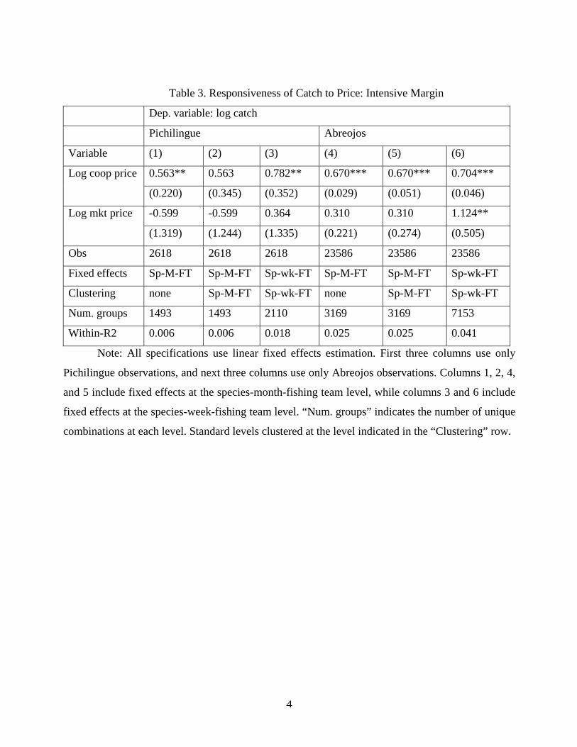
4 

Table 3. Responsiveness of Catch to Price: Intensive Margin

Dep. variable: log catch

Pichilingue Abreojos

Variable (1) (2) (3) (4) (5) (6)

Log coop price 0.563** 0.563 0.782** 0.670*** 0.670*** 0.704***

(0.220) (0.345) (0.352) (0.029) (0.051) (0.046)

Log mkt price -0.599 -0.599 0.364 0.310 0.310 1.124**

(1.319) (1.244) (1.335) (0.221) (0.274) (0.505)

Obs 2618 2618 2618 23586 23586 23586

Fixed effects Sp-M-FT Sp-M-FT Sp-wk-FT Sp-M-FT Sp-M-FT Sp-wk-FT

Clustering none Sp-M-FT Sp-wk-FT none Sp-M-FT Sp-wk-FT

Num. groups 1493 1493 2110 3169 3169 7153

Within-R2 0.006 0.006 0.018 0.025 0.025 0.041

Note: All specifications use linear fixed effects estimation. First three columns use only

Pichilingue observations, and next three columns use only Abreojos observations. Columns 1, 2, 4,

and 5 include fixed effects at the species-month-fishing team level, while columns 3 and 6 include

fixed effects at the species-week-fishing team level. “Num. groups” indicates the number of unique

combinations at each level. Standard levels clustered at the level indicated in the “Clustering” row.

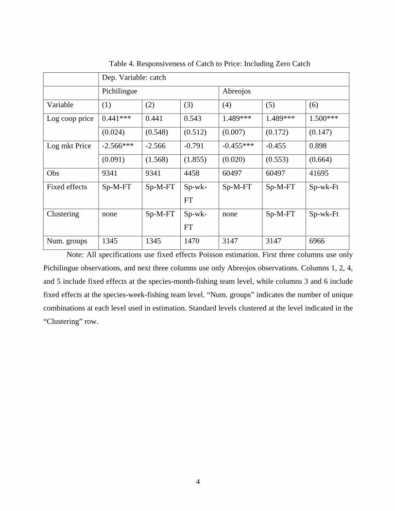
4 

Table 4. Responsiveness of Catch to Price: Including Zero Catch

Dep. Variable: catch

Pichilingue Abreojos

Variable (1) (2) (3) (4) (5) (6)

Log coop price 0.441*** 0.441 0.543 1.489*** 1.489*** 1.500***

(0.024) (0.548) (0.512) (0.007) (0.172) (0.147)

Log mkt Price -2.566*** -2.566 -0.791 -0.455*** -0.455 0.898

(0.091) (1.568) (1.855) (0.020) (0.553) (0.664)

Obs 9341 9341 4458 60497 60497 41695

Fixed effects Sp-M-FT Sp-M-FT Sp-wk-

FT

Sp-M-FT Sp-M-FT Sp-wk-Ft

Clustering none Sp-M-FT Sp-wk-

FT

none Sp-M-FT Sp-wk-Ft

Num. groups 1345 1345 1470 3147 3147 6966

Note: All specifications use fixed effects Poisson estimation. First three columns use only

Pichilingue observations, and next three columns use only Abreojos observations. Columns 1, 2, 4,

and 5 include fixed effects at the species-month-fishing team level, while columns 3 and 6 include

fixed effects at the species-week-fishing team level. “Num. groups” indicates the number of unique

combinations at each level used in estimation. Standard levels clustered at the level indicated in the

“Clustering” row.

4 

Table 5. Implication 1: Price and Catch Across Cooperatives

Log price Log catch

Variable (1) (2) (3) (4) (5) (6)

Abreojos -1.095*** -1.112*** -1.124*** 0.984*** 1.037*** 1.002***

(0.029) (0.023) (0.016) (0.183) (0.148) (0.125)

Constant 3.180*** 3.185*** 3.189*** 4.059*** 4.039*** 4.052***

(0.009) (0.007) (0.005) (0.070) (0.057) (0.048)

Obs 4310 4310 4310 5015 5015 5015

Num. groups 626 1379 3505 703 1572 4081

Within-R2 0.790 0.840 0.916 0.035 0.047 0.081

Fixed effects Sp-qtr Sp-month Sp-week Sp-qtr Sp-month Sp-week

Note: Sample includes observations at the weekly level from Abreojos, Pichilingue, and

Sargento. The omitted category is Pichilingue/Sargento. All specifications use linear fixed effects

at the species-quarter (sp-qtr), species-month (sp-month), or species-week (sp-week) level.

Standard errors are clustered at the level of the fixed effect.

5 

Table 6. Implication 2: Price/Catch Differences by Scale

Log Price Log Catch

Variable (1) (2) (3) (4) (5) (6)

Abreojos -1.174*** -1.188*** -1.187*** 1.347*** 1.354*** 1.240***

(0.029) (0.020) (0.014) (0.293) (0.217) (0.173)

Abreojos X large

scale

0.168*** 0.167*** 0.149*** -0.778** -0.705** -0.561**

(0.058) (0.046) (0.035) (0.351) (0.289) (0.246)

Constant 3.178*** 3.183*** 3.185*** 4.060*** 4.044*** 4.062***

(0.009) (0.007) (0.005) (0.069) (0.056) (0.047)

Obs 4309 4309 4309 5014 5014 5014

Num. groups 625 1378 3504 702 1571 4080

Within-R2 0.795 0.845 0.920 0.041 0.053 0.088

Fixed effects Sp-qtr Sp-month Sp-week Sp-qtr Sp-month Sp-week

Note: Sample includes observations at the weekly level from Abreojos, Pichilingue, and

Sargento. The omitted category is Pichilingue/Sargento. All specifications use linear fixed effects

at the species-quarter (sp-qtr), species-month (sp-month), or species-week (sp-week) level.

Standard errors are clustered at the level of the fixed effect.

5 

Table 7. Implication 3: Effect of Growth Rates on Price Differences

Dep Variable: Log Cooperative Price

Variable (1) (2) (3) (4) (5) (6)

Abreojos -0.780*** -0.835*** -0.960*** -1.189*** -1.181*** -1.188***

(0.133) (0.173) (0.233) (0.023) (0.032) (0.017)

Abreojos X large

scale

0.157*** 0.139*** 0.162*** 0.158*** 0.162*** 0.141***

(0.043) (0.045) (0.052) (0.044) (0.056) (0.033)

Log mkt price 0.395*** 1.022 -2.440

(0.117) (0.845) (2.406)

Abreojos X log mkt

price

-0.135*** -0.114* -0.085

(0.050) (0.060) (0.075)

Abreojos X ONI 0.056* 0.071** 0.047 0.065** 0.064* 0.064***

(0.034) (0.035) (0.045) (0.031) (0.037) (0.023)

Abreojos X recruit

effect

0.793*** 0.722*** 0.652*** 0.393*** 0.274*** 0.403***

(0.176) (0.198) (0.232) (0.063) (0.085) (0.049)

Abreojos X ONI X

recruit effect

0.211*** 0.193** 0.196** 0.208*** 0.097 0.228***

(0.074) (0.075) (0.086) (0.074) (0.090) (0.055)

Estimation method FE FE-IV FE-IV FE FE FE

Fixed effects Sp-mth Sp-mth Sp-mth Sp-mth Sp-qtr Sp-week

Obs 2871 2600 2538 2871 2871 2871

Num. groups 770 575 560 770 340 2152

Within-R2 0.905 0.902 0.876 0.941

Note: Sample includes observations at the weekly level from Abreojos, Pichilingue, and

Sargento. The omitted cooperative category is Pichilingue/Sargento. Columns 2 and 3 treat log

market price as endogenous and instrument for it using the one period and two period lag of log

market price, respectively. Standard errors are clustered at the level of the fixed effect.

5 

Appendix

In the main text, we use a fixed effects approach to examine whether fishers respond to changes in

the cooperative price as assumed in the model. A complementary approach presented here instead

examines changes in catch at the time of events when there is a large change in cooperative prices

for a species. Here, using a small window around these price changes, we control for changes in

catch associated with time trends and examine the effect of dummy variables for the onset of higher

or lower prices.

Figure 1 shows both the potential and the challenges of such an approach. The figure shows

daily log prices and catch at Abreojos for a species known colloquially as “Vieja”, which has

the fourth most entries in the Abreojos logbooks among all species. Log prices are averaged

across all entries for a day, and catch is summed over all fishing teams for a day. We include

only days on which there was at least one catch recorded. Three features of the graph are

notable. First, there is some indication that spikes in prices are occurring at the same time as

spikes in catch. This is true even in the middle of the graph, where there is a short-term spike in

prices that deviates substantially from neighboring prices. Second, while there are periods where

prices are relatively stable, they move around quite a bit over time. This makes the definition

of an “event” for an event analysis challenging. Third, catch moves around even when prices are

relatively stable. This could be because of seasonal patterns in fishing effort and natural

fluctuations in stock.

To take a systematic approach given these challenges, we do the following: We focus on

dates on which the log price is 0.2 larger or smaller than the previous seven dates in the log book

data, and then remains that distance from the previous seven values for at least six dates in the

future. The result is a 14-date window in which the seven days in the latter half of the

window have an approximately 20% higher (or 20% lower) price than the seven days in the

first half of the window.31 This criterion is satisfied at least once by only eight species in our

                                                       31 Note that the logbooks do not always have recorded catch for every single day. Therefore, the 14-date window could

5 

data, and all eight are from Abreojos (including “Vieja”).

Figure 2 show the raw price and catch data for these eight species in the event windows.32 The

figure is structured analogously to Figure 1. There is substantial noise in the data; while a few

pictures reveal a positive relationship between price and catch movements, others do not. In order

to remove time effects related to seasonality in fishing effort, we run regressions of log catch and

catch on the time variable (days since Jan. 2, 2007), the square of the time variable, a dummy

variable for a price increase regime shift, and a dummy variable for a price decrease regime shift.

The results appear in Table 1, where the first column examines log catch with a linear model, the

second examines catch with a linear model, and the third examines catch with a Poisson model (to

deal with the fact that catch is never negative and has many values close to zero). All columns use

species fixed effects. We see evidence that downward price adjustments are associated with lower

catch, and upward price adjustments are associated with higher catch, but these coefficients are

sometimes imprecisely estimated.

Given the challenges of an event analysis in this setting, we view these results as complementary

to the fixed effects analysis in the main text. Overall, the evidence suggests that catch responds to

cooperative prices in the manner assumed in the model.

                                                                                                                                                                                   include dates that are spread across more than two weeks. We restrict the window to lie within a two month span to avoid mingling different seasons into one window. 32 Species number 85, ``Jurel'', has multiple windows. The figure includes only the first two windows, which are contiguous. 

5 

Figure 1: Price and Catch Movements for “Vieja”

Vieja (Species 84)

0 200 400 Days Since Jan 2 2007

600 800

Log Price (2010 pesos) Catch (kg)

Log

Pric

e

Cat

ch (

kg)

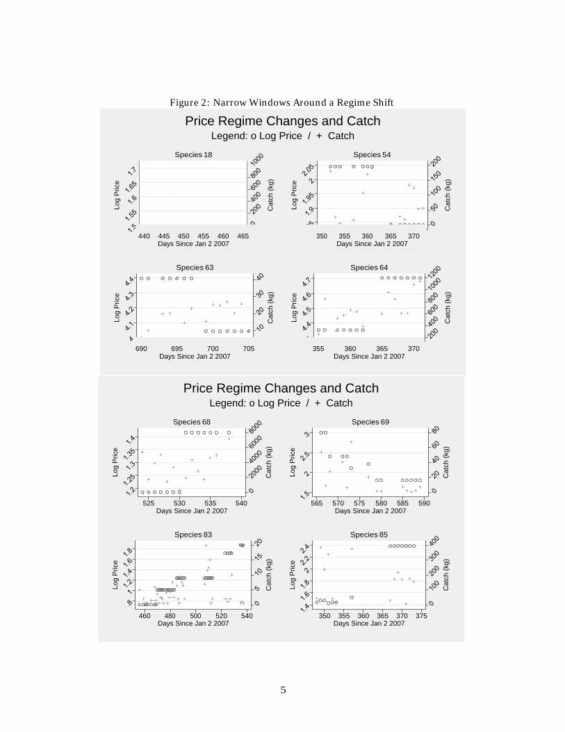
5 

Price Regime Changes and Catch Legend: o Log Price / + Catch

Species 18 Species 54

Species 63 Species 64

Price Regime Changes and Catch Legend: o Log Price / + Catch

Species 68 Species 69

525 530 535 540 565 570 575 580 585 590Days Since Jan 2 2007 Days Since Jan 2 2007

Species 83 Species 85

460 480 500 520 540Days Since Jan 2 2007

350 355 360 365 370 375Days Since Jan 2 2007

Figure 2: Narrow Windows Around a Regime Shift

690

695 700

705

355

360 365

370

  Days Since Jan 2 2007     Days Since Jan 2 2007  

Lo

g P

rice

L

og

Pri

ce

Lo

g P

rice

L

og

Pri

ce

Ca

tch

(kg

) C

atc

h (k

g)

Ca

tch

(kg

) C

atc

h (k

g)

Lo

g P

rice

L

og

Pri

ce

Lo

g P

rice

L

og

Pri

ce

Ca

tch

(kg

) C

atc

h (k

g)

Ca

tch

(kg

) C

atc

h (k

g)  

 

 

  440

445 450 455 460

465

350

355 360 365

370

  Days Since Jan 2 2007     Days Since Jan 2 2007  

5 

Table 1: Price Regime Shifts and Changes in Catch

Variable Log Catch Catch (Linear) Catch (Poisson) Price Decrease (0/1) -0.808** -19.297 -0.555***

  (0.334) (184.468) (0.052) Price Increase (0/1) 0.044 95.008 0.267***

  (0.165) (91.016) (0.008) Date 0.098 -8.660 -0.000

  (0.065) (36.042) (0.005) Date Squared -0.000 0.008 -0.000

(0.000) (0.035) (0.000) Obs 152 152 152 Num. Groups 8 8 8

NOTE: All specifications use species fixed effects and restrict to the event window, as defined in the text.