miguel a. velásquez valle - redalyc.org filerevista mexicana de ciencias agrícolas issn: 2007-0934...

Revista Mexicana de Ciencias Agrícolas

ISSN: 2007-0934

[email protected]

Instituto Nacional de Investigaciones

Forestales, Agrícolas y Pecuarias

México

Velásquez Valle, Miguel A.; Díaz Padilla, Gabriel; Muñoz Villalobos, Jesús A.; Guajardo Panes, Rafael

Alberto; Sánchez Cohen, Ignacio

Aleatoriedad de una serie de precipitación en el estado de Veracruz, México

Revista Mexicana de Ciencias Agrícolas, núm. 1, julio-agosto, 2011, pp. 41-55

Instituto Nacional de Investigaciones Forestales, Agrícolas y Pecuarias

Estado de México, México

Disponible en: http://www.redalyc.org/articulo.oa?id=263120987004

Cómo citar el artículo

Número completo

Más información del artículo

Página de la revista en redalyc.org

Sistema de Información Científica

Red de Revistas Científicas de América Latina, el Caribe, España y Portugal

Proyecto académico sin fines de lucro, desarrollado bajo la iniciativa de acceso abierto

http://www.redalyc.org/revista.oa?id=2631

http://www.redalyc.org/articulo.oa?id=263120987004

http://www.redalyc.org/comocitar.oa?id=263120987004

http://www.redalyc.org/fasciculo.oa?id=2631&numero=20987

http://www.redalyc.org/articulo.oa?id=263120987004

http://www.redalyc.org/revista.oa?id=2631

http://www.redalyc.org

Revista Mexicana de Ciencias Agrícolas Pub. Esp. Núm. 1 1 de julio - 31 de agosto, 2011 p. 41-55

ALEATORIEDAD DE UNA SERIE DE PRECIPITACIÓN EN EL ESTADO DE VERACRUZ, MÉXICO*

RANDOMNESS OF A SERIES OF PRECIPITATION IN THE STATE OF VERACRUZ, MEXICO

Miguel A. Velásquez Valle1§, Gabriel Díaz Padilla2, Jesús A. Muñoz Villalobos1, Rafael Alberto Guajardo Panes2 e Ignacio Sánchez Cohen1

1Centro Nacional de Investigación Disciplinaria en Relación Agua-Suelo-Planta-Atmósfera. INIFAP. Margen derecha Canal Sacramento, km 6.5. C. P. 35140. Gómez Palacio, Durango. ([email protected]), ([email protected]). 2Campo Experimental Cotaxtla. INIFAP. Carretera Federal Veracruz-Córdoba, km 34.5. Medellín de Bravo, Veracruz. C. P. 94270. ([email protected]), ([email protected]). §Autor para correspomdencia: [email protected].

* Recibido: febrero de 2011

Aceptado: julio de 2011

RESUMEN

Ante un eminente cambio en las tendencias de los estadísticos, que describen las series de tiempo de información climática en las últimas décadas, es necesario caracterizar adecuadamente las series de tiempo, con el propósito de aumentar el grado de predicción de las variables involucradas. El objetivo es presentar el análisis de la información pluviométrica considerando el análisis fractal, con el propósito de explicar el grado de aleatoriedad de la serie de tiempo, desde un punto de vista multiescalar en tiempo. En el estado de Veracruz, la estación meteorológica “Las Vigas” es representativa de la región conocida como Las Vigas de Ramírez y se encuentra ubicada en la zona centro del estado. La longitud de la serie de tiempo de la estación es de 85 años. A partir de esta base de datos se generaron archivos para las escalas diaria, decenal, mensual y anual. Estos mismos archivos se guardaron como series de tiempo con la extensión ∗.ts, para calcular el exponente de Hurst, utilizando los métodos de referencia de ondoletas (Hw) y el Rango Re-escalado (HR/S), diseñados para el análisis de los patrones auto-afines con el programa comercial Benoit®. Se presentan los valores del exponente de Hurst para las escalas de tiempo diario (HR/S = 0.26 y Hw= 0.22) y valores promedio

ABSTRACT

Facing an imminent change in the statistical trends that describe the time series of climate information in the past decades, it is necessary to adequately characterize the time series in order to increase the involved variables’ predictability. The aim is to present the analysis of rainfall information considering the fractal analysis in order to explain the degree of randomness of the time series from a multi-scale point of view in time. In the State of Veracruz, the weather station “Las Vigas” is representative of the region known as Las Vigas de Ramírez and is located in the center of the state. The station’s length of the time series is 85 years. From this database, daily, decadal, monthly and yearly scale files were generated. These same files are stored as time series with the extension ∗.ts to calculate the Hurst exponent, using the reference methods of wavelets (Hw) and the rescaled range (HR/S) designed for the analysis of patterns self-affine with Benoit® commercial program. The Hurst exponent´s values were presented for a daily time scale (HR/S= 0.26 and Hw= 0.22) and average values for the scales of decades (HR/S= 0.25 and Hw= 0.20), monthly (HR/S= 0.26 and Hw= 0.09) and annual (HR/S=

Miguel A. Velásquez Valle et al.42 Rev. Mex. Cienc. Agríc. Pub. Esp. Núm. 1 1 de julio - 31 de agosto, 2011

para las escalas decenal (HR/S= 0.25 y Hw= 0.20), mensual (HR/S= 0.26 y Hw= 0.09) y Anual (HR/S= 0.24 y Hw= 0.21). Ambos métodos de referencia indican un comportamiento anti-persistente de las series multiescalares de tiempo, con una tendencia a la volatilidad.

Palabras clave: anti-persistencia, exponente de Hurst, grado de aleatoriedad, precipitación.

INTRODUCCIÓN

Por la complejidad en el entendimiento del funcionamiento y estructura de algunos procesos o fenómenos de un sistema, se ha señalado que posee un comportamiento caótico o con falta de orden. Estos sistemas son extremadamente sensibles a las condiciones iníciales, por lo que pequeñas variaciones en ellas pueden hacer impredecible el comportamiento futuro (Guégan y Leroux, 2009). Este comportamiento errático es una respuesta compleja (no-lineal) del sistema en función de su dinámica en el tiempo y de su variabilidad en el espacio. La dinámica no-lineal estudia aquellos sistemas que responden de manera no proporcional a un estímulo y la magnitud de la respuesta es aparentemente impredecible (Martínez, 2000). Es por esta razón que no existe un buen ajuste entre los valores observados o simulados con la línea de tendencia de modelos como los lineales.

En este contexto, la capacidad predictiva de los modelos está limitada por diversos factores o circunstancias. Algunos errores de los modelos son atribuibles a la falta de aproximación a la realidad; es decir, al desconocimiento del funcionamiento o estructura del sistema que de desea simular (Sánchez et al., 2005). Como consecuencia, pequeños errores desde el inicio de la simulación pueden crecer durante el proceso y generar información equivocada (sub o sobreestimada). Una manera de tener una buena aproximación del sistema es conocer el tipo de estructura que lo conforma. El patrón estructural del sistema contiene información que nos permite conocer su funcionamiento y en un determinado momento entender la complejidad que está detrás del sistema; la cual produce la serie de tiempo (Sánchez, 2008).

El clima como un sistema caótico, en la actualidad y a una escala global cada año se manifiestan una serie de eventos climatológicos fuera de tiempo y espacio, que han ocasionado disturbios ecológicos, biológicos e incluso la pérdida de vidas humanas. Por el comportamiento errático,

0.24 and Hw= 0.21). Both reference methods indicate anti-persistent behavior of the multi-scalar time series, with a tendency to volatility.

Key words: anti-persistence, degree of randomness, Hurst exponent, precipitation.

INTRODUCTION

Because of the complexity in understanding the functioning and structure of some processes or phenomena of a system, it has been reported that it possessed a chaotic behavior or lack of order. These systems are extremely sensitive to the initial conditions, so that small changes can make them unpredictable for the future behavior (Guégan and Leroux, 2009). This erratic behavior is a complex response (non-linear) made by the system, based on their dynamics in time and its variability in space. The non-linear dynamic study those systems that respond at an incentive in a non-proportional way and the magnitude of the response is apparently unpredictable (Martínez, 2000). It is for this reason that there is not a good fit between observed or simulated values with the modelʼs trend line such as the linear models.

In this context, the model’s predictive ability is limited by several factors or circumstances. Some model errors are attributable to the lack of approach to reality; i. e. the lack of function or structure of the system that you want to simulate (Sánchez et al., 2005). As a result, small errors from the beginning of the simulation can grow during the process and generate wrong information (under-or overestimated). One way to get a good approximation of the system is to knowing the type of structure that it forms. The structural pattern of the system contains information that lets us know how it works and at one point, to understand the complexity behind the system itself, which produces the time series (Sánchez, 2008).

The climate as a chaotic system, currently and each year in a global scale, a series of climatic events manifest out of time and space, causing ecological disturbances, biological and even losses of human lives. Due to climate’s erratic, random and unpredictable behavior, it can be classified as a chaotic or non-linear (Lima et al., 2003). In a particular region, the variation in climate averages may

Aleatoriedad de una serie de precipitación en el estado de Veracruz, México 43

aleatorio y poco predecible del clima se puede clasificar como un sistema caótico o no-lineal (Lima et al., 2003). En particular de una región, la variación en los promedios del clima pueden ocurrir debido a pequeños cambios en el periodo, que es observable o bien cuando la ocurrencia de eventos extremos logran alterar esos promedios.

Por otro lado, la ocurrencia de eventos extremos (Wang y Zhou, 2005; Da-Quan et al., 2008; Květoň y Žák, 2008) incrementan el grado de aleatoriedad e incertidumbre del clima y por consiguiente es difícil implementar acciones de cualquier tipo, que tiendan a mitigar los efectos de una posible alteración en los patrones climatológicos. Ante un eminente cambio en las tendencias de los estadísticos que describen las series de tiempo de información climática en las últimas décadas, es necesario caracterizar adecuadamente las bases de datos, con el propósito de aumentar el grado de predicción de las variables involucradas. Una de las variables climatológicas de importancia es la precipitación pluvial. La predicción de la precipitación es útil, porque de ella dependen la mayoría de los procesos que regulan la vida en nuestro planeta.

Tradicionalmente las herramientas utilizadas en la predicción de la precipitación, están basadas en el uso de promedios, así como en otras medidas del grado de dispersión de los datos con respecto a la media, los cuales se calcularon utilizando los momentos estadísticos de segundo y tercer (desviación estándar y varianza, respectivamente) y en algunos de ellos son utilizadas probabilidades condicionadas. Los modelos para la generación de información climatológica como el ClimGen y WGen (Richardson y Wright, 1984; Nelson, 2003; respectivamente) requieren de la base de datos este tipo de estadísticos.

Estos modelos han sido de gran utilidad para proporcionar información climatológica a otros que simulan procesos hidrológicos y de erosión de suelos como el RUSLE (Yu, 2002). Sin embargo, algunas deficiencias de los modelos es que no permiten: a) caracterizar el patrón de heterogeneidad, que es una propiedad del sistema a diferentes escalas; b) describir las relaciones funcionales entre las propiedades del sistema; c) los procesos que se llevan a cabo; y d) sus mecanismos funcionales (Oleschko et al., 1997).

Desde la década de los 50’s se han desarrollado nuevos conceptos y métodos en el análisis de series de tiempo. Aunado a lo anterior, la geometría fractal ha sido una importante herramienta en la toma de decisiones en lo relacionado con el manejo de los recursos hídricos (Salomão

occur due to small changes in the period that is observable or when the occurrences of extreme events are able to alter these averages.

On the other hand, the occurrences of extreme events (Wang y Zhou, 2005; Da-Quan et al., 2008; Květoň y Žák, 2008) increase the degree of randomness and uncertainty of climate and thus are difficult to implement actions of any kind aimed at mitigating the effects of a possible change in the weather patterns. Facing an imminent change in the statistical trends that describe the time series of climate information in the past decades, it is necessary to adequately characterize the databases in order to increase the predictability of the variables involved. One of the relevant meteorological variables is the precipitation. The prediction of the precipitation is quite useful, because on it depends most of the processes that give and control life in our planet.

Traditionally, the tools used in the prediction of the precipitation are based on the use of averages, as well as other measures of the degree of dispersion of data regarding the mean, which are calculated using statistical moments of second and third (SD standard variance, respectively) and in some of them, conditional probabilities are used. The models for generating climatic information such as ClimGen and WGen (Richardson and Wright, 1984; Nelson, 2003, respectively) require the kind of statistics for the database.

These models have been useful to providing climatic information to others that simulate hydrologic and soil’s erosion processes, such as RUSLE (Yu, 2002). However, some deficiencies of these models are that they do not allow: a) to characterize the pattern of heterogeneity, which is a property of the system at different scales; b) describe the functional relationships between the properties of the system; c) the processes that take place; and d) their functional mechanisms (Oleschko et al., 1997).

Since the 50’s, new concepts and methods for the analysis of time series have been developed. Added to this, the fractal geometry has been an important tool in making decisions related to the management of water resources (Salomão et al., 2009). The fractal dimension allows to measuring how many times does the complexity is being repeated at each scale, and for a time series, it helps to explain or describe the relationship of the increases (Breslin and Belward, 1999). One way to calculate the fractal dimension is through the Hurst exponent.


et al., 2009). La dimensión fractal nos permite medir que tantas veces la complejidad está siendo repetida en cada escala y para una serie de tiempo, ayuda a explicar o describir la relación de los incrementos (Breslin y Belward, 1999); una manera de calcular la dimensión fractal es a través del exponente de Hurst.

El objetivo de este estudio es presentar un método alternativo al convencional, para analizar una serie de tiempo con información pluviométrica, con el propósito de explicar el grado de aleatoriedad de la misma, desde un punto de vista multiescalar en tiempo.

MATERIALES Y MÉTODOS

Estación climatológica “Las Vigas”

En el estado de Veracruz, la estación meteorológica “Las Vigas”, es representativa de la región conocida como Las Vigas de Ramírez y se encuentra ubicada en la zona centro, con las coordenadas 19o 38’ latitud norte y 97o 06’ longitud oeste, a una altura de 2 484 msnm. En este lugar el clima representativo es templado-húmedo-regular con una temperatura promedio anual de 1 074 mm, registrándose en promedio 97 días con lluvia al año; la temperatura promedio anual es de 25.8 oC. Su suelo es de tipo Andosol y Litosol, el primero se ha formado a partir de cenizas volcánicas y el segundo caracterizado por tener una profundidad menor de 10 cm.

Características de la serie de tiempo de precipitación

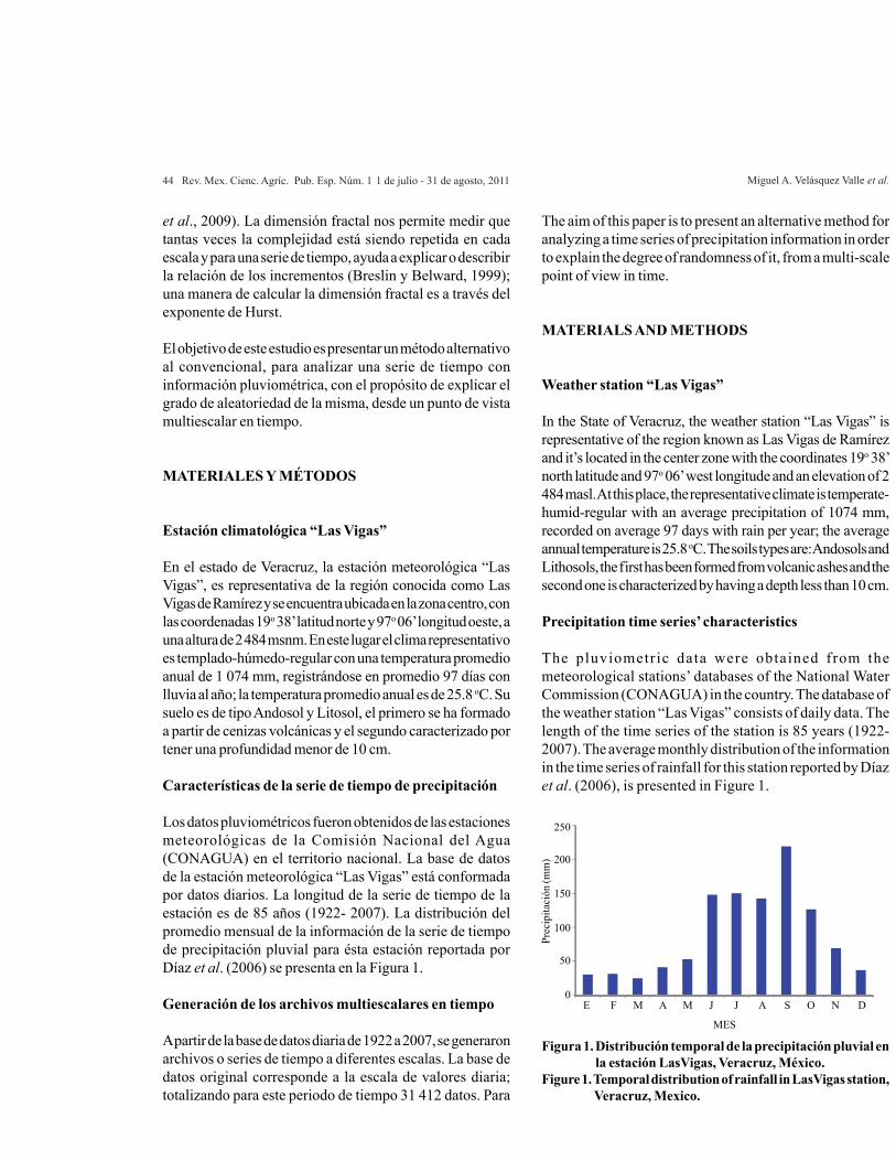
Los datos pluviométricos fueron obtenidos de las estaciones meteorológicas de la Comisión Nacional del Agua (CONAGUA) en el territorio nacional. La base de datos de la estación meteorológica “Las Vigas” está conformada por datos diarios. La longitud de la serie de tiempo de la estación es de 85 años (1922- 2007). La distribución del promedio mensual de la información de la serie de tiempo de precipitación pluvial para ésta estación reportada por Díaz et al. (2006) se presenta en la Figura 1.

Generación de los archivos multiescalares en tiempo

A partir de la base de datos diaria de 1922 a 2007, se generaron archivos o series de tiempo a diferentes escalas. La base de datos original corresponde a la escala de valores diaria; totalizando para este periodo de tiempo 31 412 datos. Para

The aim of this paper is to present an alternative method for analyzing a time series of precipitation information in order to explain the degree of randomness of it, from a multi-scale point of view in time.

MATERIALS AND METHODS

Weather station “Las Vigas”

In the State of Veracruz, the weather station “Las Vigas” is representative of the region known as Las Vigas de Ramírez and it’s located in the center zone with the coordinates 19o 38’ north latitude and 97o 06’ west longitude and an elevation of 2 484 masl. At this place, the representative climate is temperate-humid-regular with an average precipitation of 1074 mm, recorded on average 97 days with rain per year; the average annual temperature is 25.8 oC. The soils types are: Andosols and Lithosols, the first has been formed from volcanic ashes and the second one is characterized by having a depth less than 10 cm.

Precipitation time series’ characteristics

The pluviometric data were obtained from the meteorological stations’ databases of the National Water Commission (CONAGUA) in the country. The database of the weather station “Las Vigas” consists of daily data. The length of the time series of the station is 85 years (1922-2007). The average monthly distribution of the information in the time series of rainfall for this station reported by Díaz et al. (2006), is presented in Figure 1.

Figura 1. Distribución temporal de la precipitación pluvial en la estación LasVigas, Veracruz, México.

Figure 1. Temporal distribution of rainfall in LasVigas station, Veracruz, Mexico.

250

200

150

100

50

0

Prec

ipita

ción

(mm

)

E F M A M J J A S O N D

MES


la escala decenal se constituyeron archivos por cada decena del año; es decir, el primer archivo decenal correspondió a aquellos valores de precipitación que ocurrieron en los primeros diez días del mes de enero, de cada uno de los 85 años contabilizando para esta escala 860 datos.

La escala mensual se conformó con los valores de precipitación registrados para cada mes de cada año; así, el archivo del mes de enero agrupó los datos de precipitación diaria del mes de enero de 1922, hasta los valores registrados en el mes de enero de 2007 (2 666 datos) y finalmente la escala anual, está constituida por los valores de precipitación registrada cada año, abarcando de esta manera el total de valores de la serie de tiempo original. Estos mismos archivos se guardaron como series de tiempo con la extensión ∗.ts, para calcular la dimensión fractal y el coeficiente de Hurst utilizando los métodos de referencia de ondoletas (Dw) y del rango re-escalado (DR/S) diseñados para el análisis de los patrones auto-afines con el programa comercial Benoit® (Benoit, 1997).

Obtención de parámetros fractales

Método de ondoletas (Dw)

El método de ondoletas analiza las variaciones localizadas del coeficiente de Hurst, relacionando los datos mediante la descomposición de la traza (serie de tiempo) en tres armónicas dentro del espacio frecuencia-tiempo. Esta descomposición es útil para determinar los tipos de variabilidad que dominan en una serie de datos, así como su dinámica en tiempo. El método es válido para el análisis de las trazas auto-afines, donde la varianza no es constante con el incremento del tamaño de la ventana. La forma de la ondoleta se determina a tiempos espaciados y cuantificando como varía o permanece constante en el tiempo.

El algoritmo considera n transformadas de ondoleta, cada una con su propio y diferente coeficiente de escalado (ai ); donde S1, S2……..Sn son las desviaciones estándar a partir de cero de los coeficientes de escalamiento respectivo (ai).

La tasa de variación de las desviaciones estándar G1, G2…….G n - 1 se define como:

(1)

El valor promedio de Gi se estima a partir de la ecuación:

Generation of the multi-scale in time files

From the daily database from 1922 to 2007, files or time series were generated at different scales. The original database corresponds to the scale of daily values; amounting to this period of time 31 412 data. For the decadal scale, records were established for each decade of the year; i. e., the first decade file corresponded to those values of precipitation that occurred in the first ten days of January of each of the 85 years, accounting for this scale 860 data.

The monthly scale was integrated by the precipitation’s values, recorded each month of each year; so the January file grouped the daily rainfall data from January 1922 to the values recorded in the month of January 2007 (2 666 data) and finally the annual scale is formed by the precipitation’s values recorded each year, thus covering the total value of the original time series. These same files are stored as time series with the ∗.ts extension, in order to calculate the fractal dimension and the Hurst coefficient using the reference of wavelet methods (Dw) and the re-scaled range (DR/S) designed for the self-similar patterns’ analysis with the commercial software Benoit® (Benoit, 1997).

Obtaining fractal parameters

Wavelet methods (Dw)

The wavelet methods analysis the localized Hurst coefficient’s variations, relating the data by the decomposition of the trace (time series) in three harmonics, within the space frequency-time. This decomposition is useful for determining the variability types that dominate in a series of data and its dynamics in time. The method is valid for the analysis of self-affine traces, where the variance is not constant with the increasing window’s size. The wavelet’s shape is determined in spaced timings, quantifying its movements over time.

The algorithm considers n wavelet transforms, each with its own distinct scaling coefficient (ai), where S1, S2 ........ Sn, are the standard deviations parting from zero of the respective scaling coefficients (ai).

The standard deviation´s variation rate G1, G2, ......., Gn-1 is defined as:

(1)

The average value of Gi is estimated from the equation:

G1= S1, G2= S2…..........….Gn - 1= Sn - 1

S2 S3 Sn G1= S1, G2= S2…..........….Gn - 1= Sn - 1

S2 S3 Sn


(2)

El coeficiente de Hurst se calcula como:

H= f(Gpromedio) (3)

Donde: f= función heurística, que se usa para aproximar el coeficiente de Hurst por Gpromedio para las trazas estocásticas auto-afines (Benoit, 1997). De manera práctica el coeficiente de Hurst es relacionado con la dimensión fractal (D) de la siguiente manera (Carbone et al., 2004).

H= 2-D (4)

Método del rango re-escalado (R/S)

Al considerar un intervalo de una traza o serie de tiempo, es posible obtener dos parámetros: el rango de variación de la variable (R(w)) y la desviación estándar (S(w)). El primero de ellos es medido con respecto a la tendencia dentro del intervalo. Esta tendencia es estimada simplemente como la unión entre el primero y el último valor dentro del intervalo. El segundo parámetro es la desviación estándar de la primera derivada delta y de los valores de y dentro del intervalo. Las primeras diferencias entre y’ se definen como las diferencias entre los valores de y en algún punto x y otro, ubicado en una posición (x-dx) previa sobre el eje x:

dy(x)= y(x) - y(x - dx) (5)

Donde: delta x(dx) es el intervalo de muestreo; es decir, el intervalo entre los dos valores consecutivos de x que se están considerando. Una medida confiable de S(w) requiere que los datos se calculen con un intervalo de muestreo dx constante, porque se busca que las diferencias esperadas entre los valores consecutivos de y sean una función del tipo ley de potencia con la distancia (w) que los separa.

R(w)/ S(w) αwH (6)

S(w) en el método de rango re-escalado se usa para normalizar el rango R(w) para permitir comparaciones de diferentes conjuntos de datos; si no se usa S(w), el rango R(w) puede calcularse sobre los conjuntos de datos que tienen un intervalo de muestreo no-constante. El rango de re-escalado se define como:

R(w)/ S(w)= <R(w)/S(w)> (7)

(2)

The Hurst coefficient is calculated as:

H= f(Gaverage) (3)

Where: f= heuristic function, which is used to approximate the Hurst coefficient for Gaverage for the stochastic self-affine traces (Benoit, 1997). As a practical matter, the Hurst coefficient is related to the fractal dimension (D) as follows (Carbone et al., 2004):

H= 2-D (4)

Re-scaled range method (R/S)

When considering a trace interval or time series, it is possible to obtain two parameters: the variableʼs range of variation (R(w)) and the standard deviation (S(w)). The first one is measured with respect to the trend within the interval. This tendency is estimated simply as the union between the first and the last values within the interval. The second parameter is the standard deviation of the first derivative y delta of the y’s values within the interval. The first difference between y’s it’s defined as the differences between the values of y at some point x and another one located at a previous position (x-dx) over the x-axis:

dy(x)= y(x) - y(x - dx) (5)

Where: delta x(dx) is the sampling interval, i. e. the interval between two consecutive values of x that are being considered. A reliable measurement of S(w) requires that the data are calculated with a constant dx interval sampling, because it is intended that the expected differences between consecutive y values are a function of power law type with distance (w) that separates them:

R(w)/ S(w) αwH (6)

S(w) in the re-scaled range method is used to normalize the range R(w) to allowing comparisons of different data sets; if S(w) is not used, the R(w) range can be calculated on the data sets with a sampling interval not-constant. The re-scaled range is defined as:

R(w)/ S(w)= <R(w)/S(w)> (7)

n-1Gavg= ∑ Gi/n-1 i-1

n-1Gavg= ∑ Gi/n-1 i-1


Donde: w= longitud de ventana o intervalo de análisis de los datos y los paréntesis anguladas <R(w)> denotan el promedio de un número considerado de valores de R(w). En la práctica, para una determinada longitud de ventana w, uno subdivide la serie de tiempo analizada un número de intervalos de longitud w, mide R(w) y S(w) en cada intervalo, y calcula primero para cada ventana R(w)/S(w) y posteriormente la tasa promedio de <R(w)/S(w)>.

Este proceso se repite para un número de las longitudes de ventana seleccionada por el algoritmo de manera automática y el logaritmo de R(w)/S(w) es graficado versus los logaritmos de w. Si la traza es auto-afín, la gráfica debe seguir una línea recta cuya pendiente es igual al coeficiente de Hurst (H). La dimensión fractal de la traza, se calcula a partir de la relación arriba mencionada entre el coeficiente de Hurst y la dimensión fractal.

El coeficiente de Hurst

El coeficiente de Hurst mide la intensidad de dependencia entre los datos y de acuerdo con su magnitud, la serie de tiempo se clasifica como persitente (0.5< H≤ 1), lo que se interpreta que existe dependencia entre un evento y los ocurridos anteriormente; cuando se clasifica la serie de tiempo como antipersistente (0≤ H< 0.5), se puede decir que la serie está caracterizada por una tendencia a ser caótica o que sus valores tienen alta volatilidad.

En el caso de que H= 0.5 se concluye que la serie de tiempo es aleatoria y los datos no son correlacionados entre sí; es decir, donde los valores futuros de la serie no son influenciados por lo que ocurre en el presente (Palomas, 2002). Este último caso modela el ruido blanco, la distribución Gaussiana normal o el movimiento Browniano clásico. Los dos casos anteriores describen los movimientos Brownianos fraccionarios. El valor de H permite definir si el comportamiento de datos de la precipitación es persistente o anti-persistente (Burgos y Pérez, 1999; Miranda et al., 2004) y en función de esto hablar del tipo de correlación (positiva o negativa) entre los eventos.

Como parte complementaria al análisis de la información pluviométrica, se obtuvieron los estadísticos básicos que miden la tendencia central (promedio), la dispersión (desviación estándar y coeficiente de variación), así como el coeficiente de asimetría o sesgo y el grado de apuntamiento o curtosis de la serie de tiempo de lluvia.

Where: w= window’s length or range of data analysis and the angled brackets <R(w)> denote an average number of values of R(w). In practice, for a given window’s length w, one subdivides the time series analyzed a number of intervals of length w, measuring R(w) and S(w) at each interval, and each window is first calculated R(w)/S(w), then the average rate < R(w)/S(w) >.

This process is repeated for a number of window lengths selected by the algorithm automatically and the logarithm of R(w)/S(w) is plotted versus the w logarithms. If the trace is self-affine, the plot should follow a straight line whose slope is equal to the Hurst coefficient (H). The fractal dimension of the trace is calculated from the above relationship between the Hurst coefficient and the fractal dimension.

The Hurst coefficient

The Hurst coefficient measures the strength of dependence between the data and according to their magnitude the time series is classified as persistent (0.5< H≤ 1) meaning that there is a dependency between an event and the occurred earlier; when the time series is classified as anti-persistent (0≤ H< 0.5) we can say that the series is characterized by a tendency to be chaotic or that their values are highly volatile.

In the case of H= 0.5 it is concluded that the time series data is random and it’s not correlated with each other; that is where the future values of the series are not influenced for what’s happening in the present (Palomas, 2002 ). The latter case models the white noise, the normal Gaussian distribution or the classical Brownian motion. Both cases described the fractional Brownian motions. The values of H define whether the behavior of rainfall data is persistent or anti-persistent (Burgos and Pérez, 1999; Miranda et al., 2004) and according to this, define the type of correlation (positive or negative) between the events.

As a complement to the pluviometric information analysis, the basic statistics were obtained, measuring the central tendency (mean), dispersion (standard deviation and coefficient of variation) as well as the rain time seriesʼ coefficient of asymmetry or bias and the pointing degree or kurtosis.


RESULTS AND DISCUSSION

Description of the structural pattern of the time series

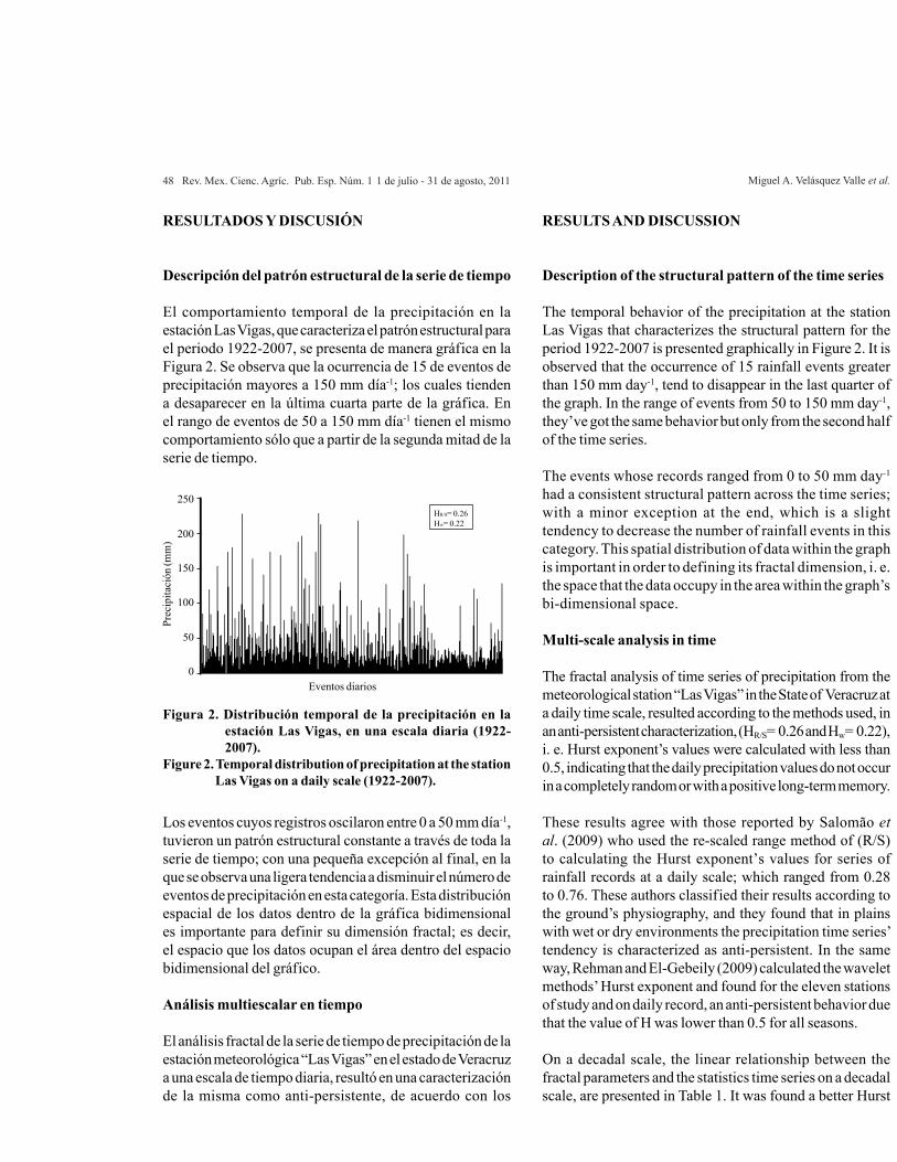
The temporal behavior of the precipitation at the station Las Vigas that characterizes the structural pattern for the period 1922-2007 is presented graphically in Figure 2. It is observed that the occurrence of 15 rainfall events greater than 150 mm day-1, tend to disappear in the last quarter of the graph. In the range of events from 50 to 150 mm day-1, they’ve got the same behavior but only from the second half of the time series.

The events whose records ranged from 0 to 50 mm day-1 had a consistent structural pattern across the time series; with a minor exception at the end, which is a slight tendency to decrease the number of rainfall events in this category. This spatial distribution of data within the graph is important in order to defining its fractal dimension, i. e. the space that the data occupy in the area within the graph’s bi-dimensional space.

Multi-scale analysis in time

The fractal analysis of time series of precipitation from the meteorological station “Las Vigas” in the State of Veracruz at a daily time scale, resulted according to the methods used, in an anti-persistent characterization, (HR/S= 0.26 and Hw= 0.22), i. e. Hurst exponent’s values were calculated with less than 0.5, indicating that the daily precipitation values do not occur in a completely random or with a positive long-term memory.

These results agree with those reported by Salomão et al. (2009) who used the re-scaled range method of (R/S) to calculating the Hurst exponentʼs values for series of rainfall records at a daily scale; which ranged from 0.28 to 0.76. These authors classified their results according to the ground’s physiography, and they found that in plains with wet or dry environments the precipitation time series’ tendency is characterized as anti-persistent. In the same way, Rehman and El-Gebeily (2009) calculated the wavelet methods’ Hurst exponent and found for the eleven stations of study and on daily record, an anti-persistent behavior due that the value of H was lower than 0.5 for all seasons.

On a decadal scale, the linear relationship between the fractal parameters and the statistics time series on a decadal scale, are presented in Table 1. It was found a better Hurst

RESULTADOS Y DISCUSIÓN

Descripción del patrón estructural de la serie de tiempo

El comportamiento temporal de la precipitación en la estación Las Vigas, que caracteriza el patrón estructural para el periodo 1922-2007, se presenta de manera gráfica en la Figura 2. Se observa que la ocurrencia de 15 de eventos de precipitación mayores a 150 mm día-1; los cuales tienden a desaparecer en la última cuarta parte de la gráfica. En el rango de eventos de 50 a 150 mm día-1 tienen el mismo comportamiento sólo que a partir de la segunda mitad de la serie de tiempo.

Los eventos cuyos registros oscilaron entre 0 a 50 mm día-1, tuvieron un patrón estructural constante a través de toda la serie de tiempo; con una pequeña excepción al final, en la que se observa una ligera tendencia a disminuir el número de eventos de precipitación en esta categoría. Esta distribución espacial de los datos dentro de la gráfica bidimensional es importante para definir su dimensión fractal; es decir, el espacio que los datos ocupan el área dentro del espacio bidimensional del gráfico.

Análisis multiescalar en tiempo

El análisis fractal de la serie de tiempo de precipitación de la estación meteorológica “Las Vigas” en el estado de Veracruz a una escala de tiempo diaria, resultó en una caracterización de la misma como anti-persistente, de acuerdo con los

Figura 2. Distribución temporal de la precipitación en la estación Las Vigas, en una escala diaria (1922-2007).

Figure 2. Temporal distribution of precipitation at the station Las Vigas on a daily scale (1922-2007).

250

200

150

100

50

0

Prec

ipita

ción

(mm

)

Eventos diarios

HR/S= 0.26Hw= 0.22


métodos de referencia utilizados (HR/S= 0.26 y Hw= 0.22); es decir, se calcularon valores del exponente Hurst menores a 0.5, lo que indica que los valores de precipitación diaria no ocurren de una manera totalmente aleatoria o con memoria positiva a largo plazo.

Estos resultados concuerdan con lo reportado por Salomão et al. (2009), quienes utilizaron el método del rango re-escalado (R/S) para calcular los valores del exponente de Hurst, para series de registros pluviométricos a una escala diaria; los cuales fluctuaron entre 0.28 a 0.76. Los autores mencionados clasificaron sus resultados en función de la fisiografía del terreno, y encontraron que para planicies con ambientes húmedos o secos la tendencia de las series de tiempo de precipitación se caracteriza por ser anti-persistente. De igual manera, Rehman y El-Gebeily (2009) calcularon el exponente de Hurst por el método de ondoletas, encontrando para las once estaciones de estudio y para un periodo de registros diarios un comportamiento anti-persistente, ya que el valor de H fue menor de 0.5 para todas las estaciones.

En una escala decenal, la relación lineal entre los parámetros fractales y los estadísticos de la serie de tiempo en una escala decenal se presentan en el Cuadro 1. Se encontró una mejor asociación del exponente de Hurst extraído de la serie de tiempo de precipitación, por el método de referencia de rango re-escalado (HR/S) con los estadísticos de la misma. Se observa que aunque el método de rango re-escalado, utiliza de inversamente proporcional la desviación estándar (ecuación 6), para estimar el exponente de Hurst, no existe una asociación significativa de este estadístico (r= - 0.2) con los valores de exponente HR/S.

Sin embargo, cuando la desviación estándar es utilizada para calcular el coeficiente de variación y de asimetría, se mejora la relación lineal con los valores decenales del exponente de Hurst. En menor proporción se observa el mismo comportamiento, cuando el exponente de Hurst es estimado por el método de ondoletas (Hw).

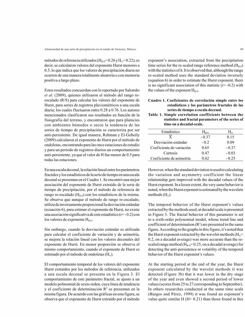
El comportamiento temporal de los valores del exponente Hurst extraídos por los métodos de referencia, utilizados a una escala decenal se presenta en la Figura 3. El comportamiento de este parámetro fractal, se ajusto a un modelo polinomial de sexto orden, cuya línea de tendencia y el coeficiente de determinación R2 se presentan en la misma figura. De acuerdo con las gráficas en esta figura, se observa que el exponente de Hurst extraído por el método

exponentʼs association, extracted from the precipitation time series for the re-scaled range reference method (HR/S) with the statistics of it. It is observed that, although the range re-scaled method uses the standard deviation inversely (equation 6) in order to estimate the Hurst exponent, there is no significant association of this statistic (r= -0.2) with the values of the exponent HR/S.

However, when the standard deviation is used to calculating the variation and asymmetry coeff icient the linear relationship gets improved with the decadal values of the Hurst exponent. In a lesser extent, the very same behavior is noted, when the Hurst exponent is estimated by the wavelets methods (Hw).

The temporal behavior of the Hurst exponent’s values extracted by the methods used, at decadal scale is presented in Figure 3. The fractal behavior of this parameter is set to a sixth-order polynomial model, whose trend line and coefficient of determination (R2) are presented in the same figure. According to the graphs in this figure, it’s noted that the Hurst exponent extracted by the wavelet methods (Hw= 0.2, on a decadal average) was more accurate than the re-scaled range method (HR/S= 0.25, on a decadal average) for detecting the anti-persistence or volatility of the temporal behavior of the Hurst exponent’s values.

At the starting period at the end of the year, the Hurst exponent calculated by the wavelet methods it was detected (Figure 3b) that it was lower in the dry stage of the year and even showed a second period of lower values (scores from 25 to 27 corresponding to September). In others researches conducted at the same time scale (Burgos and Pérez, 1999) it was found an exponentʼs value quite similar H (H= 0.21) than those found in this

Estadístico HR/S Hw

X - 0.37 0.15Desviación estándar - 0.2 0.09

Coeficiente de variación 0.65 - 0.37Curtosis 0.47 - 0.03

Coeficiente de asimetría 0.62 - 0.25

Cuadro 1. Coeficientes de correlación simple entre los estadísticos y los parámetros fractales de las series de tiempo a escala decenal.

Table 1. Simple correlation coefficients between the statistics and fractal parameters of the series of time on a decadal-scale.


de ondoletas (Hw= 0.2, como promedio decenal) fue más preciso que el método del rango re-escalado (HR/S= 0.25, como promedio decenal), para detectar la anti-persistencia o volatilidad del comportamiento temporal de los valores del exponente Hurst.

En el periodo de inicio a final del año, se detectó que el exponente de Hurst calculado por el método de ondoletas (Figura 3b), es menor en la etapa más seca del año e inclusive se observa una segunda época de bajos valores (decenas 25 a 27 que corresponden al mes de septiembre). En otras investigaciones realizadas en esta misma escala de tiempo (Burgos y Pérez, 1999) encontraron un valor del exponente H muy similar (H= 0.21) a los encontrados en este estudio. Los autores referidos estimaron el valor del exponente mediante un programa basado en que el valor esperado de (Sn)2, está relacionado de manera lineal con el valor de H; de esta manera para diferentes valores de n, el valor de la pendiente de la línea de regresión entre log n y log (Sn)2, corresponde al valor del exponente H.

Es importante señalar que el comportamiento temporal a través del año de los valores del exponente de Hurst es opuesto, dependiendo del método utilizado. La tendencia de los valores del exponente de Hurst para el periodo de la

paper. The authors referred, estimated the exponentʼs value with a program based on expecting (Sn)2 value to be linearly related to the value of H; in this way for the different values of n, the value of the slope of the line regression between log n log (Sn)2, corresponds to the value of the exponent H.

It’s noteworthy, that the temporal behavior of the Hurst exponent’s values through the year are opposite, depending on the method used. The tendency of the Hurst exponent’s values for the period from the decade 7 to 21 in Figure 3a is downwardly, whereas in Figure 3b, the values’ tendency are opposite. This behavior can be seized by the researcher, because it depends on the degree of accuracy or focus of interest.

If the purpose is to determine the maximum level of volatility in the time series, the method with which the Hurst exponent’s value is lower or close to zero should be chosen, whereas if the objective is to document the degree of randomness, the reference method with which the Hurst exponentʼs value is closest or equal to 0.5 should be selected. In order to achieve the same results of the Hurst exponentʼs values with both methods itʼs likely to needing to calibrate them before, via a standardization or transformation of the database (Table 2).

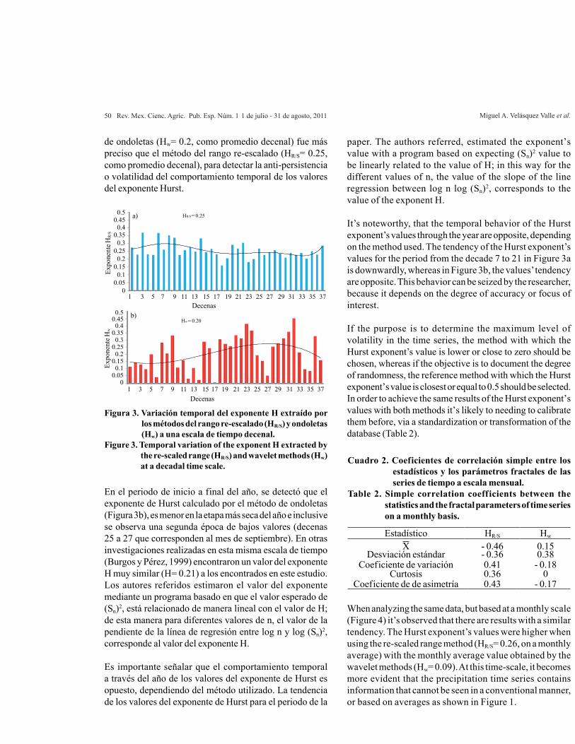
When analyzing the same data, but based at a monthly scale (Figure 4) it’s observed that there are results with a similar tendency. The Hurst exponent’s values were higher when using the re-scaled range method (HR/S= 0.26, on a monthly average) with the monthly average value obtained by the wavelet methods (Hw= 0.09). At this time-scale, it becomes more evident that the precipitation time series contains information that cannot be seen in a conventional manner, or based on averages as shown in Figure 1.

Figura 3. Variación temporal del exponente H extraído por los métodos del rango re-escalado (HR/S) y ondoletas (Hw) a una escala de tiempo decenal.

Figure 3. Temporal variation of the exponent H extracted by the re-scaled range (HR/S) and wavelet methods (Hw) at a decadal time scale.

Estadístico HR/S Hw

X - 0.46 0.15Desviación estándar - 0.36 0.38

Coeficiente de variación 0.41 - 0.18Curtosis 0.36 0

Coeficiente de de asimetría 0.43 - 0.17

Cuadro 2. Coeficientes de correlación simple entre los estadísticos y los parámetros fractales de las series de tiempo a escala mensual.

Table 2. Simple correlation coefficients between the statistics and the fractal parameters of time series on a monthly basis.

0.50.45

0.40.35

0.30.25

0.20.15

0.10.05

0

Expo

nent

e HR

/S

l 3 5 7 9 11 13 15 17 19 21 23 25 27 29 31 33 35 37

HR/S = 0.25

Decenas

a)

0.50.45

0.40.35

0.30.25

0.20.15

0.10.05

0

Expo

nent

e Hw

l 3 5 7 9 11 13 15 17 19 21 23 25 27 29 31 33 35 37Decenas

Hw = 0.20b)


decena 7 a 21 en la Figura 3a es descendente; mientras que en la Figura 3b la tendencia de los valores es en sentido contrario. Este comportamiento puede ser aprovechado por el investigador, ya que dependiendo del grado de precisión o enfoque de interés.

Sí el propósito es determinar el máximo nivel de volatilidad de la serie de tiempo, se deberá escoger el método con el cual el valor del exponente de Hurst sea más bajo o cercano a cero; pero si el objetivo es documentar el grado de aleatoriedad, se deberá seleccionar el método de referencia con el cual el valor del exponente de Hurst se aproxime o sea igual a 0.5. Para lograr consensar un mismo resultado del valor del exponente de Hurst con los dos métodos aquí utilizados, es factible la necesidad de calibrarlos previamente vía una estandarización o transformación de la base de datos (Cuadro 2).

Al analizar la misma base de datos pero a una escala mensual (Figura 4), se observa que existen resultados con una tendencia similar. Los valores del exponente de Hurst fueron mayores cuando se utilizó el método de rango re-escalado (HR/S = 0.26, como promedio mensual), con el valor promedio mensual obtenido por el método de ondoletas (Hw= 0.09). A esta escala temporal se hace más evidente que la serie de tiempo de precipitación, contiene información que no puede ser vista de una manera convencional o basada en promedios como se aprecia en la Figura 1.

A través de los resultados obtenidos por los métodos de referencia, como el rango re-escalado y ondoletas, se puede apreciar que a esta escala temporal, la información de la serie de tiempo de precipitación de la estación “Las Vigas”, tiene un comportamiento antipersistente; es decir, no tiene memoria a largo plazo. En la Figura 4b se detecta que los eventos de lluvia que ocurren en los meses previos y al final de la época de lluvia, son totalmente independientes o no dependen de los ocurridos con anterioridad, como sí puede ocurrir cuando de presentan eventos dentro de la época lluviosa del año.

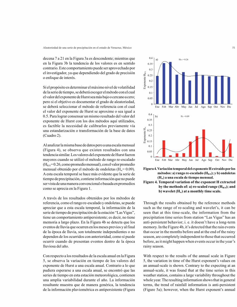
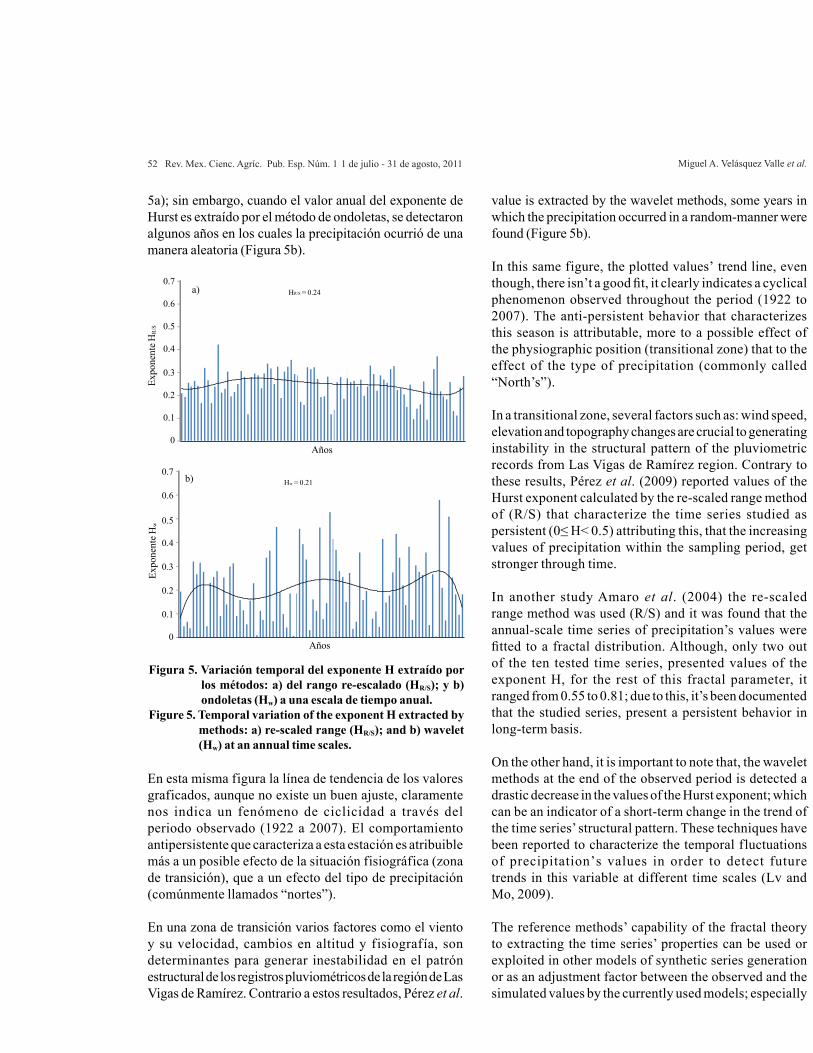
Con respecto a los resultados de la escala anual en la Figura 5, se observa la variación en tiempo de los valores del exponente de Hurst a una escala anual. Contrario a lo que pudiera esperarse a una escala anual, se encontró que las series de tiempo en esta estación meteorológica, contienen una amplia variabilidad durante el año. La información resultante muestra que de manera genérica, la tendencia de la información pluviométrica es antipersistente (Figura

Through the results obtained by the reference methods such as the range of re-scaling and wavelet’s, it can be seen that at this time-scale, the information from the precipitation time series from station “Las Vigas” has an anti-persistent behavior; i. e. it doesn’t have a long-term memory. In the Figure 4b, it’s detected that the rain events that occur in the months before and at the end of the rainy season, are completely independent to those that occurred before, as it might happen when events occur in the year’s rainy season.

With respect to the results of the annual scale in Figure 5, the variation in time of the Hurst exponent’s values on an annual-scale is shown. Contrary to the expecting at an annual-scale, it was found that at the time series in this weather station, contains a large variability throughout the whole year. The resulting information shows that in general terms, the trend of rainfall information is anti-persistent (Figure 5a); however, when the Hurst exponent’s annual

Figura 4. Variación temporal del exponente H extraído por los métodos: a) rango re-escalado (HR/S); y b) ondoletas (Hw) a una escala de tiempo mensual.

Figure 4. Temporal variation of the exponent H extracted by the methods of: a) re-scaled range (HR/S); and b) wavelet (Hw) at a monthly time scale.

0.4

0.35

0.3

0.25

0.2

0.15

0.1

0.05

0

Expo

nent

e HR

/S

a)

Ene Feb Mar Abr May Jun Jul Ago Sep Oct Nov Dic

HR/S = 0.26

b)0.4

0.35

0.3

0.25

0.2

0.15

0.1

0.05

0Ene Feb Mar Abr May Jun Jul Ago Sep Oct Nov Dic

Expo

nent

e Hw

Hw = 0.09


value is extracted by the wavelet methods, some years in which the precipitation occurred in a random-manner were found (Figure 5b).

In this same figure, the plotted valuesʼ trend line, even though, there isn’t a good fit, it clearly indicates a cyclical phenomenon observed throughout the period (1922 to 2007). The anti-persistent behavior that characterizes this season is attributable, more to a possible effect of the physiographic position (transitional zone) that to the effect of the type of precipitation (commonly called “North’s”).

In a transitional zone, several factors such as: wind speed, elevation and topography changes are crucial to generating instability in the structural pattern of the pluviometric records from Las Vigas de Ramírez region. Contrary to these results, Pérez et al. (2009) reported values of the Hurst exponent calculated by the re-scaled range method of (R/S) that characterize the time series studied as persistent (0≤ H< 0.5) attributing this, that the increasing values of precipitation within the sampling period, get stronger through time.

In another study Amaro et al. (2004) the re-scaled range method was used (R/S) and it was found that the annual-scale time series of precipitation’s values were fitted to a fractal distribution. Although, only two out of the ten tested time series, presented values of the exponent H, for the rest of this fractal parameter, it ranged from 0.55 to 0.81; due to this, it’s been documented that the studied series, present a persistent behavior in long-term basis.

On the other hand, it is important to note that, the wavelet methods at the end of the observed period is detected a drastic decrease in the values of the Hurst exponent; which can be an indicator of a short-term change in the trend of the time series’ structural pattern. These techniques have been reported to characterize the temporal fluctuations of precipitationʼs values in order to detect futuretrends in this variable at different time scales (Lv and Mo, 2009).

The reference methods’ capability of the fractal theory to extracting the time series’ properties can be used or exploited in other models of synthetic series generation or as an adjustment factor between the observed and the simulated values by the currently used models; especially

5a); sin embargo, cuando el valor anual del exponente de Hurst es extraído por el método de ondoletas, se detectaron algunos años en los cuales la precipitación ocurrió de una manera aleatoria (Figura 5b).

En esta misma figura la línea de tendencia de los valores graficados, aunque no existe un buen ajuste, claramente nos indica un fenómeno de ciclicidad a través del periodo observado (1922 a 2007). El comportamiento antipersistente que caracteriza a esta estación es atribuible más a un posible efecto de la situación fisiográfica (zona de transición), que a un efecto del tipo de precipitación (comúnmente llamados “nortes”).

En una zona de transición varios factores como el viento y su velocidad, cambios en altitud y fisiografía, son determinantes para generar inestabilidad en el patrón estructural de los registros pluviométricos de la región de Las Vigas de Ramírez. Contrario a estos resultados, Pérez et al.

Figura 5. Variación temporal del exponente H extraído por los métodos: a) del rango re-escalado (HR/S); y b) ondoletas (Hw) a una escala de tiempo anual.

Figure 5. Temporal variation of the exponent H extracted by methods: a) re-scaled range (HR/S); and b) wavelet (Hw) at an annual time scales.

Expo

nent

e HR

/S

0.7

0.6

0.5

0.4

0.3

0.2

0.1

0

a)

Años

HR/S = 0.24

Expo

nent

e Hw

b)

Años

0.7

0.6

0.5

0.4

0.3

0.2

0.1

0

Hw = 0.21


(2009) reportan valores del exponente de Hurst calculados por el método del rango re-escalado (R/S), que caracterizan las series de tiempo estudiadas como persistentes (0≤ H< 0.5), atribuyendo lo anterior a que los incrementos de los valores de precipitación dentro del periodo de muestreo se fortalecen como transcurre el tiempo.

En otro estudio, Amaro et al. (2004) se utilizó el método del rango re-escalado (R/S) y se encontró que en series de tiempo a una escala anual, los valores de precipitación se ajustaron a una distribución fractal. Aunque solo dos de las diez series de tiempo evaluadas presentaron valores del exponente H, para el resto este parámetro fractal osciló entre 0.55 a 0.81; por lo que se documenta que las series estudiadas presentan persistencia a largo plazo.

Por otro lado, es relevante señalar que por el método de ondoletas al final del periodo observado, se detecta una disminución drástica de los valores del exponente de Hurst; lo que puede ser un indicador de cambio a corto plazo en la tendencia del patrón estructural de la serie de tiempo. Estas técnicas ya han sido reportadas para caracterizar las fluctuaciones temporales de valores de precipitación, con el objetivo de detectar tendencias a futuro de esta variable a diferentes escalas de tiempo (Lv y Mo, 2009).

Esta capacidad de los métodos de referencia de la teoría fractal de extraer propiedades de las series de tiempo, puede ser utilizada o aprovechada en otros modelos de generación de series sintéticas o bien como un factor de ajuste entre los valores observados y simulados, por los modelos que actualmente son utilizados; principalmente cuando no se observa el fenómeno de invarianza al escalado espacial o temporal. La generación de estos modelos “híbridos” debe ser validada aún más cuando se presenta en la actualidad, un incremento en el grado de incertidumbre en la predicción de variables climáticas.

Invarianza al escalado en tiempo

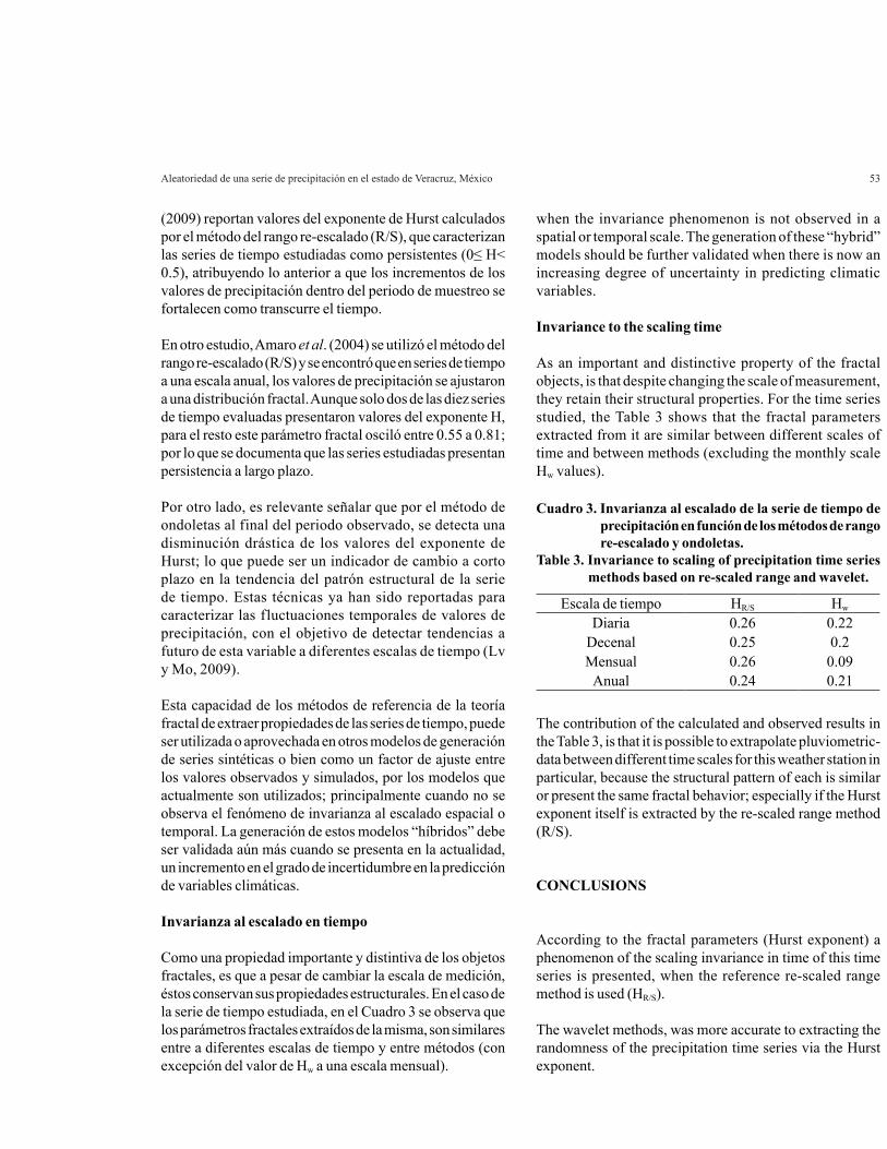
Como una propiedad importante y distintiva de los objetos fractales, es que a pesar de cambiar la escala de medición, éstos conservan sus propiedades estructurales. En el caso de la serie de tiempo estudiada, en el Cuadro 3 se observa que los parámetros fractales extraídos de la misma, son similares entre a diferentes escalas de tiempo y entre métodos (con excepción del valor de Hw a una escala mensual).

when the invariance phenomenon is not observed in a spatial or temporal scale. The generation of these “hybrid” models should be further validated when there is now an increasing degree of uncertainty in predicting climatic variables.

Invariance to the scaling time

As an important and distinctive property of the fractal objects, is that despite changing the scale of measurement, they retain their structural properties. For the time series studied, the Table 3 shows that the fractal parameters extracted from it are similar between different scales of time and between methods (excluding the monthly scale Hw values).

The contribution of the calculated and observed results in the Table 3, is that it is possible to extrapolate pluviometric-data between different time scales for this weather station in particular, because the structural pattern of each is similar or present the same fractal behavior; especially if the Hurst exponent itself is extracted by the re-scaled range method (R/S).

CONCLUSIONS

According to the fractal parameters (Hurst exponent) a phenomenon of the scaling invariance in time of this time series is presented, when the reference re-scaled range method is used (HR/S).

The wavelet methods, was more accurate to extracting the randomness of the precipitation time series via the Hurst exponent.

Escala de tiempo HR/S Hw Diaria 0.26 0.22

Decenal 0.25 0.2 Mensual 0.26 0.09 Anual 0.24 0.21

Cuadro 3. Invarianza al escalado de la serie de tiempo de precipitación en función de los métodos de rango re-escalado y ondoletas.

Table 3. Invariance to scaling of precipitation time series methods based on re-scaled range and wavelet.


La aportación de los resultados calculados y observados en el Cuadro 3, es que existe la posibilidad extrapolar información pluviométrica entre diferentes escalas de tiempo, para esta estación meteorológica en particular, debido que el patrón estructural de cada una de ellas es similar o tiene el mismo comportamiento fractal; espacialmente sí el exponente de Hurst es extraído por el método del rango re-escalado (R/S).

CONCLUSIONES

De acuerdo a los parámetros fractales (exponente de Hurst), se presenta un fenómeno de invarianza al escalado en tiempo de esta serie de tiempo, cuando es utilizado el método de referencia rango de re-escalado (HR/S).

El método de ondoletas fue más preciso, para extraer la aleatoriedad de la serie de tiempo de precipitación vía el exponente de Hurst.

Es necesario presentar información generada por un modelo “híbrido” de esta variable, en la cual se utilice el valor del exponente de Hurst, como un parámetro adicional a los estadísticos básicos y comparar el grado de precisión en la predicción pluviométrica, al utilizar un generador de series de tiempo “híbrido” y el comúnmente utilizado o convencional.

LITERATURA CITADA

Amaro, I. R.; Demey, J. R y Macchiavelli, R. 2004. Aplicación del análisis r/s de Hurst para estudiar las propiedades fractales de la precipitación en Venezuela. INCI. 29:617-620.

Benoit, M. 1997. Ver. 1.2 Copyright© TruSoft Intʼl Inc. 1997-1999. All Rights Reserved.

Breslin, M. C. and Belward, J. A. 1999. Fractal dimension for rainfall time series. Mathematics and Computers in Simulation. 48:437-446.

Burgos, T. R. and Pérez, V. E. 1999. Estimation of the fractal dimension of a rainfall time series over a zone relevant to the agriculture in Havana. SOMETCUBA. Bulletin. Vol. 5. Núm. 1.

Carbone, A. G.; Castelli, J. and Stanley, H. 2004. Analysis of clusters formed by the moving average of a long-range correlated time series. Phys. Rev. E69:026105. 4 p.

It’s necessary to present information generated by a “hybrid” model of this variable, in which the Hurst exponent’s value is used as an additional parameter to the basic statistics and compare the degree of accuracy in predicting precipitation, using a “hybrid” time series generator and the commonly used.

Da-Quan, Z. F.; Guo, L. and Jing, G. H. 2008. Trend of extreme precipitation events over China in last 40 years. Chinese Phys. B. 17:736-742.

Díaz, P. G.; Ruíz, C. J. A.; Cano, G. M. A.; Serrano, A. V. y Medina, G. G. 2006. Estadísticas climáticas básicas del estado de Veracruz (1961-2003). Campo Experimental Cotaxtla. INIFAP-CIRGOC. Veracruz, México. Libro técnico. Núm. 13. 292 p.

Květoň, V. and Žák, M. 2008. Extreme precipitation events in the Czech Republic in the context of climate change. Adv. Geosci. 14:251-25.

Lima, M. I.; João, L. M. P. and Coelho, E. S. 2003. Spectral analysis of scale invariance in the temporal structure of precipitation in Mainland Portugal. Eegenharia Civil. UM. 16:73-82.

Lv, J. B. S. and Mo, S. 2009. Multiple time scales analysis of precipitation in Holtan, China. J. Sustainable Development. 2:182- 85.

Martínez, M. G. 2000. Una aproximación a los sistemas complejos. Ciencias. 59:6-9.

Miranda, J. G. V.; Andrade, A. B.; da Silva, C. S.; Ferreira, A. P.; González, R. F. S. and Carrera-López, J. L. 2004. Temporal and spatial persistence in rainfall records from Northeast Brazil and Galicia, Spain. Theor. Appl. Climatol. 77:113- 21.

Nelson, R. 2003. CLIMGEN-climatic data generator. Washington State Univ., Pullman. URL: http://www.bsyse.wsu.edu/climgen/.

Oleschko, L. K.; Miranda, M. E y Prat, C. 1997. Análisis fractal de los tepetates. In: Memorias del III Simposio Internacional sobre Suelos Volcánicos Endurecidos. Quito, Ecuador. 90-97 p.

Guégan, D. and Leroux, J. 2009. Forecasting chaotic systems: the role of local Lyapunov exponents. Chaos, Solitons & Fractals. 41:2401-2404.

End of the English version


Pérez, S. P.; Sierra, E. M.; Massobrio, M. J. y Momo, F. R. 2009. Análisis fractal de la precipitación en el este de la Provincia de la Pampa, Argentina. Revista de Climatología. 9:25-31.

Rehman, S. and El-gebeily, M. 2009. A study of climatic parameters using climatic predictability indices. Chaos, Solitons and fractals. 41:1055-1069.

Richardson, C. W. and Wright, D. A. 1984. WGEN. A model for generating daily weather variables, USDA ARS Bulletin No. ARS-8. Washington DC, USA. Government Printing Office. 83 pp.

Palomas, M. E. 2002. Evidencia e implicaciones del fenómeno Hurst en el mercado de capitales. Gaceta de Economía. Año 8. 5:117-53.

Sánchez, P. A. and Velázquez, J. 2005. Nonlinear time series with breaks in the seasonal pattern. A modeling approach using neural networks. In: 25th International Symposium on Forecasting. San Antonio, TX, USA. 85 p.

Sánchez, P. A. 2008. Cambios estructurales en las series de tiempo: una revisión del estado del arte. Revista Ingenierías. 7:15-140.

Wang, Y. and Zhou, L. 2005. Observed trends in extreme precipitation events in China during 1961-2001 and the associated changes in large-scale circulation, Geophys. Res. Lett. 32, L09707, doi:10.1029/2005GL022574.

Yu, B. 2002. Using CLIMGEN to generate RUSLE climate imputs. Transactions of the ASAE. 45:993-1001.

miguel a. velásquez valle - redalyc.org filerevista mexicana de ciencias agrícolas issn: 2007-0934...

Documents