1

Control de robot móviles

INF-383Seminario de Modelo y Métodos

CuantitativosProf. Teddy Alfaro

Modelado de Sistemas

• El sistema de un robot se representa por unconjunto de variables reales satisfaciendo una igualdad o inigualdad

• A las variables se les llama variables de estado• Y al conjunto de variables que cumplen con

todas la restricciones se les llama espacio deestado

2

Teoría de control en robot móviles

• Sistema dinámico, variables de control u el

segundo término se le llama drift• Si• Es integrable, el sistema es holonómico• Si no lo es es no-holónomico

( ) ( ) ( ))()(),()(),()( 0 tuYtutxYtutxftx +==&

( ) 0,, =txxG &

Punto de vista de control

• La holonomicidad-noholonomicidad puede ser vista como– Direcciones en la cuales el movimiento es

permitido– (más que) las direcciones en las cuales el

movimiento es prohibido• Cuestionamiento

– Dado dos puntos arbitrarios, existe una trayectoria q(t) la cual satisfaga las restricciones cinemáticas

3

Representación Vectorial• Dependiendo de los grados de libertad del

sistema, se tendrán matrices y vectores

• La matriz de vectores Xi debe cumplir ciertas propiedades

• Supongamos, que nuestra es x tienda a cero (típico error)

• La solución a este sistema será la Ley de control,en este caso una solución conveniente es:

∑+= )()(0 xXuxXx ii&

xKu ⋅=& ikxiii exku −→−=

( )( )k

m

uuuuxxxx

L

L

,,,,,

21

21

==

Modelo Uniciclo

• Las variables de control son:– Velocidad traslacional – Variación de cambio angular

ωθ

θυθυ

=

==

&

&

&

sincos

yx

υω

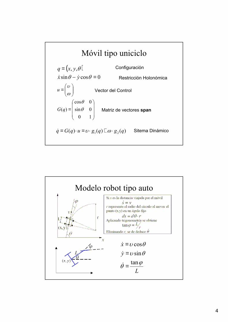
4

Móvil tipo uniciclo

( )0cossin

,,=−

=θθ

θyxyxq&&

=

=

100sin0cos

)( θθ

ωυ

qG

u

)()()( 21 qgqguqGq ⋅+⋅=⋅= ωυ&

Configuración

Restricción Holonómica

Vector del Control

Matriz de vectores span

Sitema Dinámico

Modelo robot tipo auto

L

yx

ϕθ

θυθυ

tansincos

=

==

&

&

&

5

Móvil tipo Auto( )

( ) ( )0cossin

0cossin,,,

=−

=+−+=

θθ

ϕθϕθϕθ

yxyx

yxq

ff

&&

&&

=

=

1000sin0cos

)(L

tagqG

u

ϕθθ

ϖν

( ) )()( 21 qgqguqGq ⋅+⋅=⋅= ϖν&

Configuración

RestricciónesHolonómica

Vector del Control

Matriz de vectores span

Sitema Dinámico

Matriz con singularidad en 2πϕ ±=

Controlabilidad• Condición de rango del algebra de Lie en un

punto p0

• Con es constantey

• Entonces el sistema no-holonómico será controlable si n0=n

• Lie Bracket

( ){ }mgggLiegpgSpanp ,...,,:)()( 2100 ∈=∆

( ) 00 )( npDim =∆

( ) npDim =

[ ] 12

21

21 )(, gqgg

qgqgg

∂∂

−∂∂=

6

Verificado el sistema uniciclo• Dimensión de q es 3• Dimensión de span es la

Se generan hasta 3 gi independientes. Luego, dimensión del Spande Lie(g1,g2)=dim(q) Entonces, es posible encontrar una ley decontrol para que conduzca el sistema desde cualquier estado acualquier otro estado

),,( θyxq =( ) ?),(dim 21 =ggLie

[ ]

−==

=

=

0cossin

,100

0sincos

21321 θθ

θθ

ggggg

Desarrollo anterior

Sólo se obtienen 3 gi

7

Verificando el sistema auto• Dimensión de q es 4• Dimensión del span de Lie(g1,g2)?

( )ϕθ ,,, yxq =

=

=

1000

0

tansincos

21 gL

g ϕθθ

Utilizando Lie Bracket

[ ] [ ]

−

==

−==

00cos

coscos

sin

,

0cos

100

, 2

2

3142

213 ϕθ

ϕθ

ϕL

L

gggL

ggg

Luego, dimensión del Span de Lie(g1,g2)=4=dim(q). Entonces, es posibleencontrar una ley de control para que conduzca el sistema desde cualquier estado a cualquier estado

Desarrollando• Calcular g3, resulta ser ortogonal

g3=[g1,g2]• Luego, verificar que se puede obtener g4

g4=[g1,g3]• g1,g2,g3,g4 independientes, se cumple que

la dimension 4 es equivalente a verificar el rango de la matriz span [g1 g2 g3 g4] se completo

8

Trajectory Tracking (unicycle)

ωθ

θυθυ

=

==

&

&

&

sincos

yx

refref

refrefref

refrefref

yx

ωθ

θυ

θυ

=

=

=

&

&

&

sin

cos

• Error x-xref, y-yref, - refθ θ

Trajectory Tracking

• Siguiendo el modelo cinemático, si es el error

• Debieramos obtener una expresión paray reescribir

• Luego encontrar una ley de control • Se obtiene K, y luego debe probarse que el

término driftless tiende a cero

),,( refrefref yyxxg θθ −−−=g&

∑ ⋅+= ugXgXg i )()(0&

gKu ⋅=

9

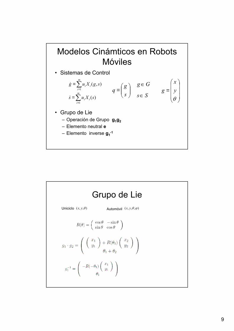
Modelos Cinámticos en Robots Móviles

• Sistemas de Control

• Grupo de Lie– Operación de Grupo g1g2

– Elemento neutral e– Elemento inverse g1

-1

∑=

=m

iii sXus

1)(&

∑=

=m

iii sgXug

1),(&

=sg

q

=θyx

gSs∈

Gg∈

Grupo de Lie),,( θyx ),,,( ϕθyxUniciclo Automóvil

10

Leyes de Control

• El cómo obtener leyes de control queda fuera del contenido del presente curso

• A continuación veremos un método moderno llamado funciones transversales

• La idea es controlar el errordonde f es una función armónica. A este enfoque se denomia Practical Stabilization

fggz r −−≈

El contenido que sigue, es sólo de tipo cultural y no preguntable para la prueba

Theorem

• X1,….,Xm Q vector field. Then the following properties are equivalent:– Lie(X1,…,Xm)(q)=TqQ (controllability)– For any neighborhood U of q in Q, there exist a

function such that, for any

∈

);( UTcf p∞∈

pT∈θ

{ } ( )pmf TdffXfXspanT )())(()),...,((1)( θθθθ ⊕=

∑=

=n

iii qXuq

1)(&

...“Practical Stabilization”, J.C. Samson, P. Morin, 2003.

11

Practical Stabilization

=

−

sggg v

1~ 1)(~ −⋅= αfgz

−−

=

r

r

rr

f yyxx

Rgθ

θ )(

Control Design on Lie Group

• Concept the transverse function used in control laws for systems

• Dynamic feedback law

• Yields the satisfaction of the equation

( )),~()()()~()( )(1

1 tgPzZzdrgdlHu

fz −=

−

−−

ααα&

∑=

+=m

iii tgPgXug

1),~()~(~&

)(zZz =& ii zk−

12

Transversality Condition

• Considering the tranversality matrix

• Inverse defined for all

( ) ( )nnnm

mfffXfXH

×+

∂∂

∂∂=

αα

ααααα )(,...,)(,)(,...,)()(

11

mnT −∈α

[ ] 0)( ≠αHDet

Examples

13

Unicycle Case

• Kynematic Equation

• Error Definition

• Practical Stabilization

• Transverse Function

+

=

100

0sincos

ωθθ

vg&

ggg r ⋅= −1~

1)(~ −⋅= αfgz

=

αε

αεε

αε

α

cos42sin

sin

)(

1

21

1

f

Unicycle

• Control Law

• Lie Group

• Linearization

( ))(),(),~()()( 11 zZfzAtgPzBHv

−− +−=

α

αω

( )ftgPzBfXfvXfzAz && −++= ),~()()()(),( 21 ω

−−−

=

33

22

11

zkzkzk

z&

14

Car-like Vehicle Case

+

=

1000

0

tansincos

ωϕθθ

Lvg&

⋅=−

ϕggg r

1~

• Kynematics Equation

• Error Definition

• Practical Stabilization 1)(~ −⋅= αfgz

Car-like• Transverse Function C.S. dim 4

• Transverse Function car-like vehicle

• Condition

15

Car-like• Control Law

• Not completely on the Lie Group

• Linearization

( ))(),(),~()()( 11

2

1

zZfzAtgPzBH

v

−− +−=

α

ααω

( ))(),~()()()(),( 21 zvCftgPzBfXfvXfzAz +−++= && ω

)(),()2/tan(2

44

33

22

11

zCfzvA

zkzkzkzk

z +

−−

−−

=&

Car-like convergence

• A(z,f) bounded matrix

=

0

00

)(4z

zc

)0()( 444 zetz tk−=

16

N-Trailer System

N-Trailer

• Standard N-Trailer vs. General N-Trailer

17

Remark• Standard N-trailer can be transformed into

chained form• Standard case has already been widely studied

but there exist few result for the general case, and the existing solutions always require some assumptions on the reference trajectory

• Motivation:– a solution with the Transversal Function

Approach – that does not require such assumptions.

Control Variables

• Change speed matrix

• with

18

1-Trailer System

Kynematics

• Kynematic Equations

• 2 control variable

• Doing

19

Rewrite system

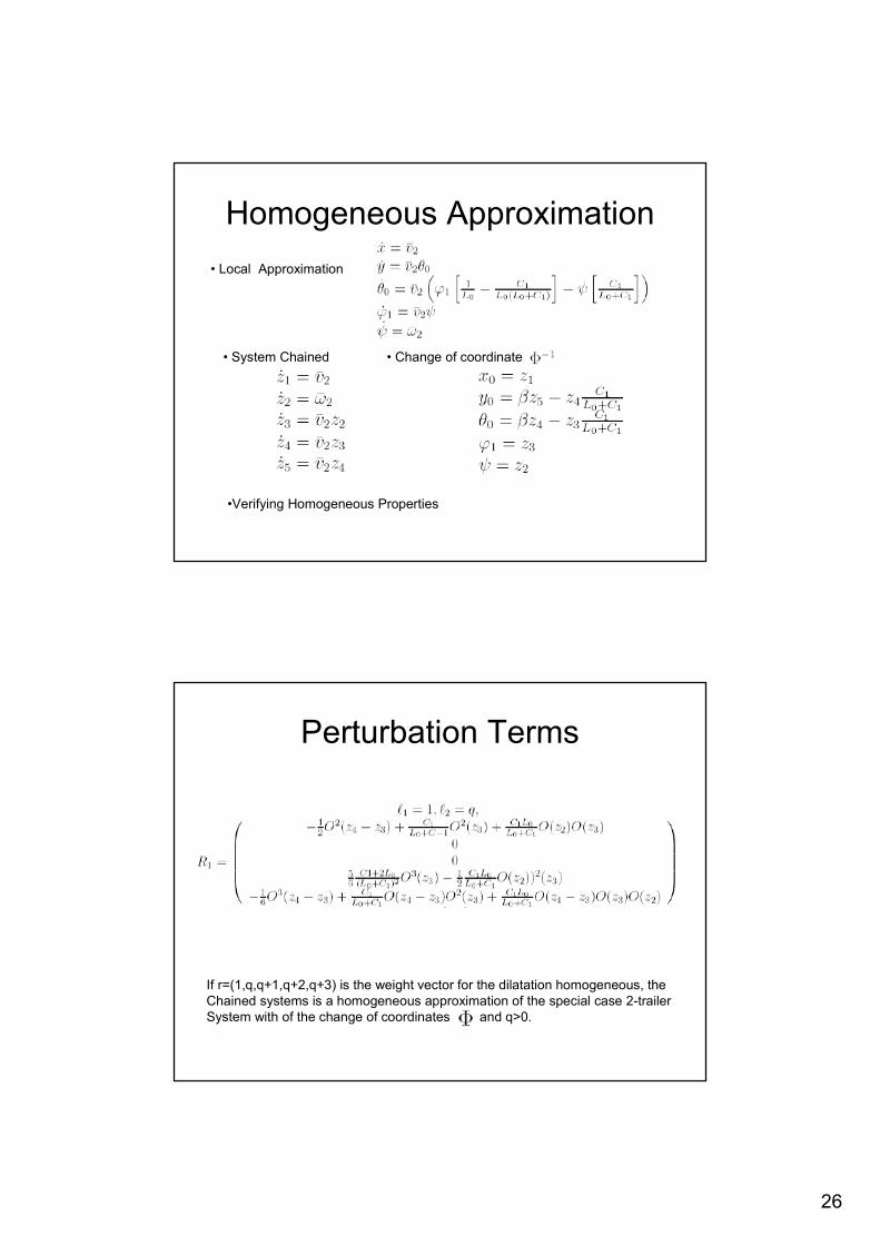
Homogeneous Approximation

• System Chained

• Local Approximation

• Homogeneous Properties

ψ• Change of coordinate

20

Perturbation Terms

If r=(1,q,q+1,q+2) is the weight vector for the dilatation homogeneous, the Chained systems is a homogeneous approximation of the system 1-trailerWith of th change of coordinates and q>1.ψ

Transverse Function

1−ψWith

Condition

21

Control Design• Error

• With

• and

Control Law

22

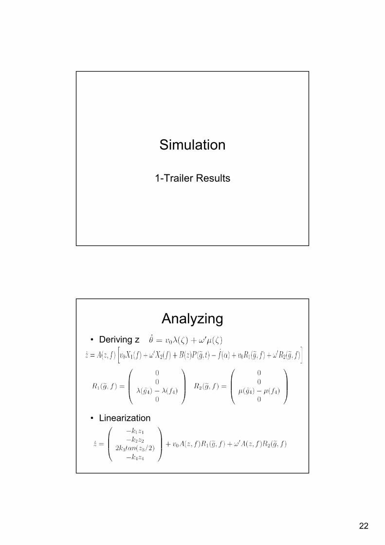
Simulation

1-Trailer Results

Analyzing• Deriving z

• Linearization

23

Convergence

• If thenFor this converge to zero

Special Case 2-Trailer System

24

Kynematics

• Kynematic Equations

• Writing all in function of the speeds),( 22 ωv

Kynematic General

• Considering

25

Special Case

• Simplifying, we study the case when C2=0

Rewrite system

26

Homogeneous Approximation

• System Chained

• Local Approximation

•Verifying Homogeneous Properties

• Change of coordinate

Perturbation Terms

If r=(1,q,q+1,q+2,q+3) is the weight vector for the dilatation homogeneous, the Chained systems is a homogeneous approximation of the special case 2-trailer System with of the change of coordinates and q>0.

27

Transverse Function

With

Control Design• Error

• With

• and

28

Control Law

Transversality Condition

• Hard condition for the parameters

29

Simulation

2-Trailer Results

Analyzing• Deriving z

• Linearization

30

Convergence

• z4,y z5

Convergence

• Third term

31

Annex

1-trailer figure

32

2-trailer figure