DOCUMENTOS DE TRABAJO

Determinants of Household Position within Chilean Wealth Household’s Distribution

Felipe MartínezFrancisca Uribe

N° 827 Septiembre 2018BANCO CENTRAL DE CHILE

BANCO CENTRAL DE CHILE

CENTRAL BANK OF CHILE

La serie Documentos de Trabajo es una publicación del Banco Central de Chile que divulga los trabajos de investigación económica realizados por profesionales de esta institución o encargados por ella a terceros. El objetivo de la serie es aportar al debate temas relevantes y presentar nuevos enfoques en el análisis de los mismos. La difusión de los Documentos de Trabajo sólo intenta facilitar el intercambio de ideas y dar a conocer investigaciones, con carácter preliminar, para su discusión y comentarios.

La publicación de los Documentos de Trabajo no está sujeta a la aprobación previa de los miembros del Consejo del Banco Central de Chile. Tanto el contenido de los Documentos de Trabajo como también los análisis y conclusiones que de ellos se deriven, son de exclusiva responsabilidad de su o sus autores y no reflejan necesariamente la opinión del Banco Central de Chile o de sus Consejeros.

The Working Papers series of the Central Bank of Chile disseminates economic research conducted by Central Bank staff or third parties under the sponsorship of the Bank. The purpose of the series is to contribute to the discussion of relevant issues and develop new analytical or empirical approaches in their analyses. The only aim of the Working Papers is to disseminate preliminary research for its discussion and comments.

Publication of Working Papers is not subject to previous approval by the members of the Board of the Central Bank. The views and conclusions presented in the papers are exclusively those of the author(s) and do not necessarily reflect the position of the Central Bank of Chile or of the Board members.

Documentos de Trabajo del Banco Central de ChileWorking Papers of the Central Bank of Chile

Agustinas 1180, Santiago, ChileTeléfono: (56-2) 3882475; Fax: (56-2) 3882231

Documento de Trabajo

N° 827

Working Paper

N° 827

Determinants of Household Position within Chilean Wealth

Household’s Distribution

Felipe Martínez Central Bank of Chile

Francisca Uribe Central Bank of Chile**

Abstract

This paper analyzes the distribution of net wealth, its relationship with income and the factors that influence the household position within the wealth distribution in Chile. The research draws on microdata from the Survey of Household Finances 2014. We de.ne net wealth as the difference between assets and debts without considering pension wealth. The results show that wealth is unequally distributed among Chilean households. In fact, 73% of wealth is owned by the richest quintile. In addition, we show that to finance partial or totally the main residence with a subsidy has a significant effect on the probability of a household being above the lowest wealth quintile and that inheritances significantly increase the probability of belonging to a higher quintile of wealth. In terms of income we show that, even though it has a significant effect in the wealth position of a household, the relationship between income and wealth is weak.

Resumen

Este documento estudia la distribución de riqueza neta, su relación con el ingreso y los factores que influyen en la posición de los hogares en la distribución de riqueza en Chile. El estudio utiliza información de la Encuesta Financiera de Hogares 2014. Definimos riqueza neta como la diferencia entre activos y pasivos sin considerar los fondos de pensiones del hogar. Los resultados muestran que la riqueza neta está desigualmente distribuida entre los hogares chilenos. De hecho, 73% de la riqueza se concentra en el quintil más rico. Además, mostramos que la utilización de subsidios para financiar parcial o totalmente la vivienda principal tiene un efecto significativo sobre la probabilidad de que un hogar esté sobre el quintil más bajo de riqueza y que recibir una propiedad como herencia aumenta significativamente la probabilidad de pertenecer a los quintiles de riqueza más altos. En relación al ingreso, mostramos que, aunque este tiene un efecto significativo en la posición en la distribución de riqueza, su relación con la riqueza es débil en el corte transversal.

The views expressed in this paper are exclusively those of the authors and do not necessarily reflect the position of the Central Bank of Chile or it’s Board members. Any errors or omissions are the responsibility of the authors. Emails: fmartinez@bcentral.cl, furibe@bcentral.cl . ** No longer works at the Central Bank of Chile.

1 Introduction

The emergence of new sources of information about the balance sheet of households and thepublication of several articles that find an increase in the wealth inequality in the last decades hasencouraged the study of wealth distribution (Wolff, 2010; Jantti, 2008; Brandolini et al., 2004). Inaddition, the publication of “The Capital in the Twenty-First Century”by Piketty (2014) and theresults of the “Commission on the Measurement of Economic Performance and Social Progress”led by Stiglitz at al. (2009) have given an important stimulus to research about household wealth.

In general, the literature has studied household wealth according to two lines of research. Onehas analyzed the distribution of wealth, and the other one has studied the determinants of wealthaccumulation.

Related to the study of wealth distribution, using the balance sheet information of householdsfrom the Survey of Consumer Finances (SCF) conducted by the US Federal Reserve Board,Kennickell (2003), Díaz-Giménez et al. (2011) and Wolff (2010) study the wealth distribution ofUS American families. All authors observe a high concentration of wealth within the richest 20%of households in different waves of the survey. In the case of Canada, Brzozowski et al. (2010)analyze the distribution of income, consumption and wealth over the past 30 years using differentsources of information.1 Their main result is that wage and income inequality has intensifiedduring the last 30 years, and that wealth inequality has remained fairly stable and fairly highsince 1999.

In the case of Europe, the Household Finance and Consumption Survey (HFCS) led by theEuropean Central Bank (ECB) has been used. Caju (2013) examines the structure, distributionand components of household wealth for countries in the HFCS. The author concludes that netwealth is more unevenly distributed than income and that there are significant disparities be-tween Eurozone countries. Using the same survey, Sierminska and Medgyesi (2013) compare theinequality of wealth and income between countries in the Eurozone and decompose the wealthin order to identify the factors that determine this inequality. The main result of their paperindicates that there are large differences not only in terms of wealth level but also in terms ofwealth inequality among the countries analyzed. Meanwhile, Kontbay-Busun and Peichl (2015)examine the joint distribution of income and wealth at the top tail of 15 Eurozone countries’distributions. Their results show a weak correlation between income and wealth.

Based on the Luxembourg Wealth Study Database (LWS),2 Cowell et al. (2012) examine thedifferences in the distribution of household wealth according to several economic and demographiccharacteristics for countries like Finland, Italy, Sweden, the United Kingdom and the UnitedStates. The authors note that the differences in wealth distribution between countries cannot beexplained away by differences in age, working status, household structure, education or income.

1The Canadian surveys used by the authors are the Survey of Familiar Expenditure, the Survey of HouseholdsSpending, the Survey of Consumer Finances, the Survey of Labour and Income Dynamics, and the Survey ofFinancial Securities.

2The Luxembourg Wealth Study consists of harmonised national data on topics like wealth, income and labourmarkets for 10 countries: Austria, Canada, Cyprus, Germany, Finland, Italy, Norway, Sweden, the United Kingdomand the United States.

1

Using the same survey, Jantti et al. (2008) develop a study of the joint distribution of income andwealth for households in Canada, Germany, Italy, Sweden and the United States. In particular,they note that net wealth and disposable income of households are highly - but not perfectly -correlated within each country.

In the case of Chile, few studies have been developed to analyze wealth distribution. Forinstance, Cox et al. (2006) study the concentration of assets and debts in Chilean householdsusing the Social Protection Survey 2004. The authors find a strong concentration of these twovariables in households with higher incomes. Meanwhile, Bauducco and Castex (2013) comparethe distribution of wealth between Chile and the United States using the financial survey for eachcountry.3 The authors find a more unequal income distribution in Chile but a greater wealthinequality in the United States. Martínez and Uribe (2017) study the distribution of net wealthand its components across Chilean households based on the SHF 2011-12. The authors find a highconcentration of wealth in the richest quintile of the population; they also conclude that wealthdistribution is more unequal than income distribution, and that there is no strong relationshipbetween wealth and income.

A second line of research that has been fostered in recent years is the study of the determinantsof wealth accumulation. Leitner (2015) studies the sources of inequality in households’gross, netand real estate gross wealth across eight Eurozone countries based on the HFCS. The main resultis that dispersion in bequest and inter-vivos transfers obtained by households has a remarkableeffect on wealth inequality. Using the same survey, Fessler and Schürz (2015) examine the roleof inheritances, income and welfare-state policies in explaining differences in household wealthwithin and between Eurozone countries. The main result is that social services provided by thestate are substitutes for private wealth accumulation and partly explain the observed differencesin the level of net wealth of households across European countries. Arrondel et al. (2014) studythe relationship between wealth and income distribution of households for 15 European countriesusing the HFCS. They conclude that to belong to the upper income deciles or to have receivedgifts or inheritances increases the probability of being in a higher wealth decile. Mathä et al.(2014) provide an in-depth analysis of factors contributing to the accumulation of householdwealth across Eurozone countries using the HFCS. The results reveal large differences in wealthwithin these countries. The main factors behind these differences are home ownership, propertyprice dynamics and intergenerational transfers. Meanwhile, Pfeffer and Griffi n (2015) study thedeterminants of extreme fluctuations in wealth in the United States using the Panel Study ofIncome Dynamics 2005 and 2007. The authors conclude that the initial wealth is a good predictorof future fluctuations, and that a large part of these fluctuations may be associated with assetsportfolio.

In the Chilean case, there are no studies analyzing the determinants of household wealthaccumulation. In that sense, our paper is a contribution about this issue for Chile. In particular,we study the determinants of the household’s position in the wealth distribution. For this purpose,we estimate a generalized ordered logit model using as the dependent variable the wealth quintileof a household. In addition, we analyze if the weak relationship between income and wealth foundby Martínez and Uribe (2017) remains when we control for other variables.

3For Chile, the authors use the Survey of Household Finances (SHF) 2007, while they use the SCF 2007 for theUnited States.

2

The paper is organized as follows. In Section 2, we describe the dataset and the clasiffi cationsused across the paper. In Section 3, we analyze the wealth distribution of Chilean households. InSection 4, we study the relationship between the distribution of wealth and income. In Section5, we describe the empirical model, and in Section 6 we analyze the results of the estimation.Section 7 presents our concluding remarks.

2 Data

For this paper, we use the microdata comes from the SHF 2014 managed by the Central Bank ofChile. This is a cross-sectional survey and provides a comprehensive sight of households’balancesheets. In particular, the survey provides data on income, assets and debts, along with the socio-demographic characteristics of the Chilean households and their members. This survey has anurban national representativeness and its fieldwork was between July 2014 and February 2015.During that period, 4,502 Chilean households were interviewed. In order to better capture thebehavior of households with the highest participation in financial markets, the sample design of theSHF oversampled the richest 20% of households in the population, its group is defined according tothe assessed value available in the sampling frame of the survey (Encuesta Financiera de Hogares,2015b).4

When we analyze the results of household surveys, we must take into account some issues.First, the SHF is a self-reported survey. This implies that the collected data may be subject to ameasurement error, which is not necessarily systematic. Second, it should be noted that althoughthe SHF tries to sample the entire population, it is likely that extremely wealthy householdsrefuse to respond. In fact, Eckerstorfer et al. (2015) present evidence that rich households areless likely to participate in surveys about household wealth based on the SCF data. This lowparticipation of the richest households might have an impact on the shape of the upper tail of thewealth distribution. Finally, since the data collected by the SHF is given voluntarily, it is diffi cultto collect complete information in all items of the survey. In order to solve the item non-responseproblem, the SHF carries out a multiple imputation process.5

It is worth mentioning that the SHF does not collect information on mandatory pension fundsfor each household member. Because of that, our measure of wealth does not incorporate thistype of assets. Martínez and Uribe (2017) show that the exclusion of mandatory pension fundshas a negative effect in the wealth inequality for Chilean households.

The main variables that we use in our work are income, assets, debts, net wealth and inher-itances of households. In the case of household income, we use the monthly disposable income,which refers to the total sum of labor income, pension income, income from financial investmentsand other incomes that are not included in the previous categories.

4This sample design is also used in the SCF from the United States (Kennickell and Woodburn, 1997) and insome countries from the HFCS (Eurosystem Household Finance and Consumption Network, 2013).

5A similar procedure is used by SCF (Kennickell, 1998) and HFCS (Eurosystem Household Finance and Con-sumption Survey, 2013).

3

Regarding assets, they are the sum of financial and non-financial assets of a household. Fi-nancial assets are defined as the sum of the amount invested in assets with variable return plusthe amount invested in assets with fixed return,6 while non-financial assets are defined as the sumof the self-reported values of the main residence, other real estate properties and vehicles.7 ,8

On the other hand, debts are the sum of mortgage and non-mortgage debt of households. Mort-gage debt includes the debt of the principal residence and other properties, while non-mortgagedebt includes consumer debt in banks and other type of formal financial institutions,9 vehicledebt, educational debt and other debts.10

Thus, the net wealth of a household is defined as the sum of assets minus debts, excludingthe funds in the mandatory pension system.11 This definition of wealth is the same used by theOrganization for Economic Cooperation and Development (OECD) in its analysis of wealth formember countries (OECD, 2015) and is of widespread used in the literature about householdwealth.

The results that are shown hereinafter are expressed in United States dollars of 2014. Thestatistical unit for the analysis of wealth distribution is the household.12 Our results are presentedfollowing the guidelines propose by the “OECD Guidelines for Micro Statistics on HouseholdWealth” (OECD, 2013). This guide classifies households according to the information of thereference person and to the household level information.13

3 Wealth Distribution

In this section, we analyze the wealth distribution of the Chilean households. The Table 1 charac-terizes the wealth distribution. In particular, the first column shows the percentage of householdsin each cetegory. The second column shows the percentage of household with negative wealth,and the third column displays the proportion of wealth in each category. Finally, fourth and fifthcolumns show the median and the interquartile range of wealth distribution, respectively.

6Financial assets are the sum of the following categories: stocks, mutual funds and other investment funds,currency and deposits, savings accounts, voluntary individual life insurance and private pension funds, net equityin own unincorporated enterprises and other assets.

7Other real estate properties are farm land, vacation properties, sheds, second residence, commercial premisesor offi ces, hotel or lodging, warehouses and parking lots.

8The reported value for the principal residence and other real estate properties is obtained from the question:“If you sell this property today, what do you think would be its value? (residence plus land)” in the questionnaireof the SHF (Encuesta Financiera de Hogares, 2015a).

9Other type of formal financial institutions are department stores, the credit unions and the family allowancecompensation funds.10Other debt includes loans from family, pawnshop, informal lenders and some other secondary sources of funding.11Through the paper we will use the terms wealth and non-previsional wealth interchangeably to refer to net

household wealth.12The SHF defines a household as a group of individuals who live in the same home and share the same budget

(single-person households are also considered). This definition is very similar to the one used in the SCF and theHFCS (Bricker et al., 2014; Eurosystem Household Finance and Consumption Network, 2013).13For more details on the definition of the reference person, see Appendix A.

4

The results in Table 1 indicate that the median household has a net wealth of around 31,000dollars, and 15% of households shows a negative level of wealth. Regarding the wealth quintiles,Table 1 shows that the richest quintile concentrates 73% of wealth.14 This result describes astrong concentration of wealth among Chilean households, which is comparable to countries likeAustria, Germany, and the United States, where the richest 20% holds over 70% of householdwealth15 (Carrol et al., 2014; Vermeulen, 2014; Díaz-Giménez et al., 2011). In terms of dispersionwithin wealth quintile, we note that the first 4 quintiles show low dispersion in wealth, while therichest quintile shows large heterogeneity for this measure. This result evidences that the largestdifferences in wealth are concentrated among the wealthiest households in the population.

In terms of the age of the reference person, Table 1 shows that the median level of wealthgrows along this variable, even over 65 years old. This is due to our wealth measure does notinclude pension wealth. We also observe that the proportion of wealth grows with the age of thereference person during her working life but it starts to decrease once the reference person reachesthe age of retirement. Moreover, we note that wealth is concentrated (24%) in the group wherethe reference person is aged between 55 and 64 years. Meanwhile, the group with the lowestwealth is represented by households whose reference person is younger than 35 holding only 8%of wealth, and has the highest proportion of households with negative wealth. Indeed, 25% ofthis group have more debts than assets. This percentage decreases with the age of the referenceperson until turning 65 years, and, thenceforth, the proportion of households with negative wealthfalls below to 10%. In terms of dispersion, we observe a large heterogeneity in wealth stocks inthe groups where the reference person is older than 54. In fact, this dispersion reaches its peakin the group led by the reference person aged over 74 years. This growth in the dispersion acrossthe age of the reference person denotes heterogeneous patterns in the accumulation of householdwealth over time.

In terms of the housing status, the results show that households who have already paid fortheir principal residence concentrate 71% of wealth and represent 45% of total households. Asimilar situation is observed in countries such as Finland, Italy, the United Kingdom and theUnited States (Cowell et al., 2012). From Table 1, we also highlight that 37% of households thatdo not own the property where they live shows negative net wealth.

Finally, we note a similar median level of wealth among households who are the outright ownersof their property and for those who are still paying for it. This result seems counterintuitivebecause owners without mortgage should show a level of wealth higher than those who are stillpaying for their home. However, this is not so because some portion of outright owners obtainedtheir property through social programs, which implies that the value of those proporties is low.Besides the latter, households who own such properties have a low capacity to generate income,which prevents them from further accumulating wealth over time. Meanwhile, the group ofhouseholds that are still paying for their house shows a low level of wealth because some of themare in the early years of their mortgage loan. Therefore, given the composition of each group, we

14Since the cut point for the first wealth quintile is zero and around 8% of households have zero wealth, it wasnecessary to generate a random assignment of households with zero wealth in order to balance the number ofhouseholds between the first and second quintiles.15 In fact, Davies et al (2011) show that the richest 10% of world population concentrates the 71% of global wealth.

5

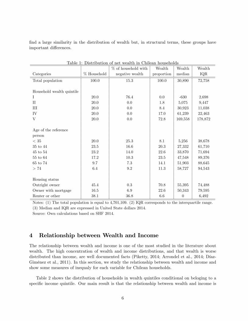
find a large similarity in the distribution of wealth but, in structural terms, these groups haveimportant differences.

Table 1: Distribution of net wealth in Chilean households% of household with Wealth Wealth Wealth

Categories % Household negative wealth proportion median IQR

Total population 100.0 15.3 100.0 30,890 72,758

Household wealth quintileI 20.0 76.4 0.0 -630 2,698II 20.0 0.0 1.8 5,075 9,447III 20.0 0.0 8.4 30,923 11,038IV 20.0 0.0 17.0 61,239 22,463V 20.0 0.0 72.8 169,558 178,872

Age of the referenceperson< 35 20.0 25.3 8.1 5,256 38,67835 to 44 23.5 16.6 20.3 27,332 61,71045 to 54 23.2 14.0 22.6 33,870 71,69455 to 64 17.2 10.3 23.5 47,548 89,37665 to 74 9.7 7.3 14.1 51,903 88,645> 74 6.4 9.2 11.3 58,727 94,543

Housing statusOutright owner 45.4 0.3 70.8 55,395 74,488Owner with mortgage 16.5 6.9 22.6 50,343 79,595Renter or other 38.1 36.8 6.6 0 6,492

Notes: (1) The total population is equal to 4,701,109. (2) IQR corresponds to the interquartile range.(3) Median and IQR are expressed in United State dollars 2014.Source: Own calculations based on SHF 2014.

4 Relationship between Wealth and Income

The relationship between wealth and income is one of the most studied in the literature aboutwealth. The high concentration of wealth and income distributions, and that wealth is worsedistributed than income, are well documented facts (Piketty, 2014; Arrondel et al., 2014; Díaz-Giménez et al., 2011). In this section, we study the relationship between wealth and income andshow some measures of inequaly for each variable for Chilean households.

Table 2 shows the distribution of households in wealth quintiles conditional on beloging to aspecific income quintile. Our main result is that the relationship between wealth and income is

6

not strong. This means that belonging to a particular income quintile does not determine thebelonging to a particular wealth quintile in the cross-sectional data, except for the richest quintile.The result in Table 2 indicates that the 80% of households with the lowest income shows a highdegree of homogeneity in wealth, since the probability of being in the first four wealth quintilesis similar. This result is similar to that found by Arrondel et al. (2014) for European countriesusing the HFCS, and by Martínez and Uribe (2017) for Chile using the SFH 2011-12.

Table 2: Joint distribution of income and wealth across household quintiles% of households in % of households in quintiles of net wealthquintiles of income I II III IV V Total

I 24.7 21.8 26.9 16.5 10.1 100II 24.7 19.9 23.5 22.5 9.3 100III 24.5 24.5 22.7 18.3 10.0 100IV 15.7 20.2 16.6 25.2 22.4 100V 10.4 13.7 10.2 17.5 48.2 100

Source: Own calculations based on SHF 2014.

To deepen the above results, in Table 3 we characterize the distributions of wealth and incomeby quintiles for each of these variables. In terms of wealth quintiles, the results show that wealthand income are concentrated in the richest quintile of the population. The proportion of wealthin this quintile reaches 73%, while the proportion of income reaches only 40%. We can also inferfrom Table 3 that, while there is an increase of the median wealth for the first three quintiles,their median level of income does not show a large variation. This may be because these quintilesconcentrate a large proportion of households whose employed members are located in the middleand the lower ranges of wages and salaries.

When we analyze the income quintiles, we note that even though the lowest quintile holdsonly 3% of the total income, it has a proportion of wealth similar to the second and third quintile.Using the SHF 2011-12, Martínez and Uribe (2017) show that this result is mainly explained by ahigh proportion of the reference persons over 65 years in the first income quintile, who own theirmain residence and have a low level of debt. From Table 3, we can also observe that the highestincome quintile holds 47% of the wealth and 58% of the income. However, the concentration ofwealth in income quintiles is less severe than the one observed in wealth quintiles.

To conclude this section, we examine some measures of inequality of income and wealth dis-tributions. The results for the different measurements are shown in Table 4. The first and mostextended measure considered is the Gini coeffi cient.16 In the case of wealth, the index reaches avalue of 0.74, which is consistent with the fact that the richest 20% of Chilean households con-centrates the 73% of non-previsional wealth. This result shows that wealth in Chile is unequallydistributed. This is also true in other countries such as Austria, Germany, and the United States,which show a Gini index above 0.70 for net wealth (Arrondel et al., 2014; Díaz-Giménez et al.,

16Since net wealth can be negative, the Gini index in this case is not bounded by 1 in the top (Chau-Nan et al.,1982).

7

2011). For income, the Gini coeffi cient reaches a value of 0.54. This result implies that wealthis worse distributed than income. It is worth mentioning that this outcome is not particular toChile. In fact, Jantti et al. (2008) point out that in many cases the wealth inequality ranking ofcountries differs considerable from the rank in terms of income inequality. Comparing our resultsto those of the United States and countries from the Eurozone, we detect that the patterns ofincome and wealth inequality are very similar to the ones observed in Chile. In particular, wenote that Chile’s wealth inequality is comparable to Austria and Germany 17(Arrondel et al.,2014; Sierminska and Medgyesi, 2013) and has one of the highest Gini indexes in terms of incometogether with the United States18 (Díaz-Giménez et al., 2011).

Table 3: Distribution of wealth and income by quintiles of wealth and incomeWealth Income

Categories Proportion Median Proportion Median

Total population 100.0 30,890 100.0 1,338

Household wealth quintileI 0.0 -630 13.6 1,083II 1.8 5,075 14.9 1,254III 8.4 30,923 13.5 1,052IV 17.0 61,239 17.9 1,373V 72.8 169,558 40.0 2,821

Household income quintileI 11.6 21,489 3.3 405II 10.5 24,046 7.4 824III 10.9 20,060 11.9 1,343IV 20.3 42,011 19.5 2,156V 46.8 86,209 57.9 4,689

Note: Median is expressed in United State dollars 2014.Source: Own calculations based on SHF 2014.

In addition, Table 4 shows that the coeffi cient of variation indicates a greater dispersion inthe distribution of wealth (2.24) than in the distribution of income (1.55). Regarding the ratiobetween the mean and the median in each distribution, we note that the ratio for wealth is higherthan the ratio for income, which indicates that wealth distribution is more concentrated thanincome distribution towards higher values. Regarding the ratio between the 90th percentile andthe median, we see that households in the 90th percentile of the distribution have almost six timesthe median level of household wealth and almost four times the median level of household income.Therefore, wealth shows a more skewed and unequal distribution than income.

17Both countries, Austria and Germany, register a Gini coeffi cient of wealth equal to 0.76. These results corre-spond to 2010-2011 (Arrondel et al., 2014).18The United States registers a Gini index of income of 0.58. These results correspond to 2007 (Díaz-Giménez et

al., 2011).

8

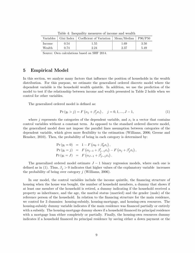
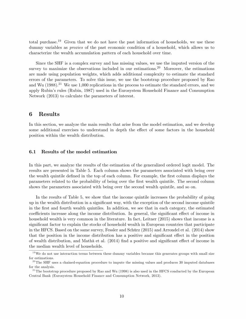
Table 4: Inequality measures of income and wealthVariables Gini Index Coeffi cient of Variation Mean/Median P90/P50

Income 0.54 1.55 1.69 3.50Wealth 0.74 2.24 2.37 5.49

Source: Own calculations based on SHF 2014.

5 Empirical Model

In this section, we analyze many factors that influence the position of households in the wealthdistribution. For this purpose, we estimate the generalized ordered discrete model where thedependent variable is the household wealth quintile. In addition, we use the prediction of themodel to test if the relationship between income and wealth presented in Table 2 holds when wecontrol for other variables.

The generalized ordered model is defined as:

Pr (yi > j) = F(αj + β

′jxi), j = 0, 1, ..., J − 1, (1)

where j represents the categories of the dependent variable, and xi is a vector that containscontrol variables without a constant term. As opposed to the standard ordered discrete model,the generalized model does not impose the parallel lines assumption between categories of thedependent variable, which gives more flexibility to the estimation (Williams, 2006; Greene andHensher, 2010). Then, the probability of being in each category is determined by:

Pr (yi = 0) = 1− F(α0 + β

′0xi),

Pr (yi = j) = F(αj−1 + β

′j−1xi

)− F

(αj + β

′jxi),

Pr (yi = J) = F(αJ−1 + β

′J−1xi

).

The generalized ordered model estimate J − 1 binary regression models, where each one isdefined as in (1). Thus, βj > 0 indicates that higher values of the explanatory variable increasesthe probability of being over category j (Williams, 2006).

In our model, the control variables include the income quintile, the financing structure ofhousing when the house was bought, the number of household members, a dummy that shows ifat least one member of the household is retired, a dummy indicating if the household received aproperty as inheritance, and the age, the marital status (married) and the gender (male) of thereference person of the household. In relation to the financing structure for the main residence,we control for 3 dummies: housing-subsidy, housing-mortgage, and housing-own resources. Thehousing-subsidy dummy variable indicates if the main residence was financed partially or entirelywith a subsidy. The housing-mortgage dummy shows if a household financed its principal residencewith a mortgage loan either completely or partially. Finally, the housing-own resources dummyindicates if a household financed its principal residence by saving either a down payment or the

9

total purchase.19 Given that we do not have the past information of households, we use thesedummy variables as proxies of the past economic condition of a household, which allows us tocharacterize the wealth accumulation pattern of each household over time.

Since the SHF is a complex survey and has missing values, we use the imputed version of thesurvey to maximize the observations included in our estimations.20 Moreover, the estimationsare made using population weights, which adds additional complexity to estimate the standarderrors of the parameters. To solve this issue, we use the bootstrap procedure proposed by Raoand Wu (1988).21 We use 1,000 replications in the process to estimate the standard errors, and weapply Rubin’s rules (Rubin, 1987) used in the Eurosystem Household Finance and ConsumptionNetwork (2013) to calculate the parameters of interest.

6 Results

In this section, we analyze the main results that arise from the model estimation, and we developsome additional exercises to understand in depth the effect of some factors in the householdposition within the wealth distribution.

6.1 Results of the model estimation

In this part, we analyze the results of the estimation of the generalized ordered logit model. Theresults are presented in Table 5. Each column shows the parameters associated with being overthe wealth quintile defined in the top of each column. For example, the first column displays theparameters related to the probability of being over the first wealth quintile. The second columnshows the parameters associated with being over the second wealth quintile, and so on.

In the results of Table 5, we show that the income quintile increases the probability of goingup in the wealth distribution in a significant way, with the exception of the second income quintilein the first and fourth wealth quintiles. In addition, we see that in each category, the estimatedcoeffi cients increase along the income distribution. In general, the significant effect of income inhousehold wealth is very common in the literature. In fact, Leitner (2015) shows that income is asignificant factor to explain the stocks of household wealth in European countries that participatein the HFCS. Based on the same survey, Fessler and Schürz (2015) and Arrondel et al. (2014) showthat the position in the income distribution has a positive and significant effect in the positionof wealth distribution, and Mathä et al. (2014) find a positive and significant effect of income inthe median wealth level of households.19We do not use interaction terms between these dummy variables because this generates groups with small size

for estimations.20The SHF uses a chained-equation procedure to impute the missing values and produces 30 imputed databases

for the analysis.21The bootstrap procedure proposed by Rao and Wu (1998) is also used in the HFCS conducted by the European

Central Bank (Eurosystem Household Finance and Consumption Network, 2013).

10

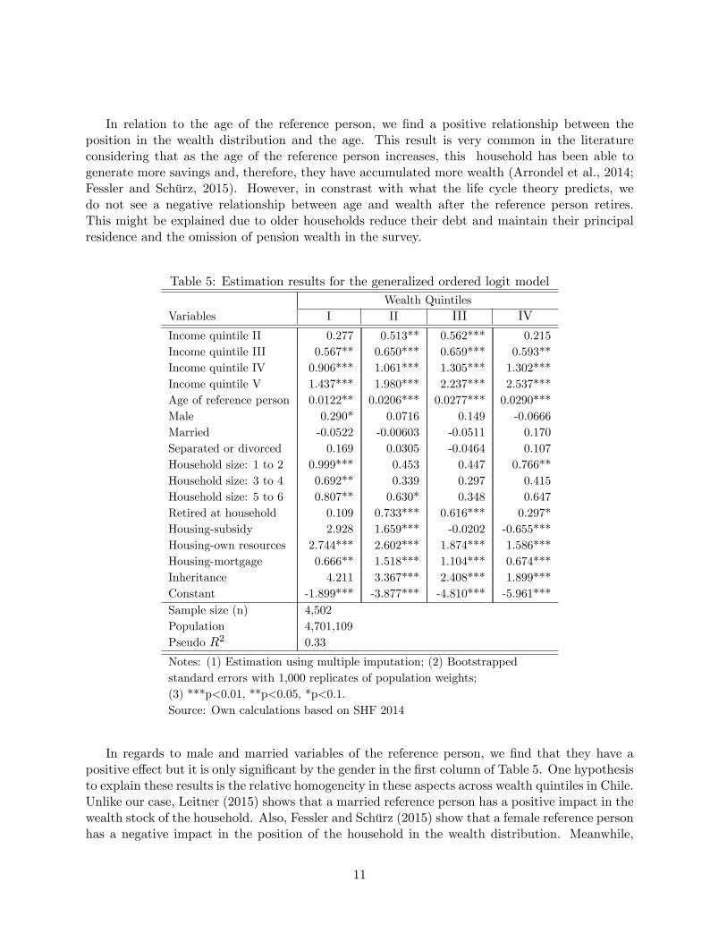
In relation to the age of the reference person, we find a positive relationship between theposition in the wealth distribution and the age. This result is very common in the literatureconsidering that as the age of the reference person increases, this household has been able togenerate more savings and, therefore, they have accumulated more wealth (Arrondel et al., 2014;Fessler and Schürz, 2015). However, in constrast with what the life cycle theory predicts, wedo not see a negative relationship between age and wealth after the reference person retires.This might be explained due to older households reduce their debt and maintain their principalresidence and the omission of pension wealth in the survey.

Table 5: Estimation results for the generalized ordered logit modelWealth Quintiles

Variables I II III IV

Income quintile II 0.277 0.513** 0.562*** 0.215Income quintile III 0.567** 0.650*** 0.659*** 0.593**Income quintile IV 0.906*** 1.061*** 1.305*** 1.302***Income quintile V 1.437*** 1.980*** 2.237*** 2.537***Age of reference person 0.0122** 0.0206*** 0.0277*** 0.0290***Male 0.290* 0.0716 0.149 -0.0666Married -0.0522 -0.00603 -0.0511 0.170Separated or divorced 0.169 0.0305 -0.0464 0.107Household size: 1 to 2 0.999*** 0.453 0.447 0.766**Household size: 3 to 4 0.692** 0.339 0.297 0.415Household size: 5 to 6 0.807** 0.630* 0.348 0.647Retired at household 0.109 0.733*** 0.616*** 0.297*Housing-subsidy 2.928 1.659*** -0.0202 -0.655***Housing-own resources 2.744*** 2.602*** 1.874*** 1.586***Housing-mortgage 0.666** 1.518*** 1.104*** 0.674***Inheritance 4.211 3.367*** 2.408*** 1.899***Constant -1.899*** -3.877*** -4.810*** -5.961***Sample size (n) 4,502Population 4,701,109Pseudo R2 0.33

Notes: (1) Estimation using multiple imputation; (2) Bootstrappedstandard errors with 1,000 replicates of population weights;(3) ***p<0.01, **p<0.05, *p<0.1.Source: Own calculations based on SHF 2014

In regards to male and married variables of the reference person, we find that they have apositive effect but it is only significant by the gender in the first column of Table 5. One hypothesisto explain these results is the relative homogeneity in these aspects across wealth quintiles in Chile.Unlike our case, Leitner (2015) shows that a married reference person has a positive impact in thewealth stock of the household. Also, Fessler and Schürz (2015) show that a female reference personhas a negative impact in the position of the household in the wealth distribution. Meanwhile,

11

Mathä et al. (2014) find a positive and significant effect over the median wealth level if thereference person is a male, and they find a mixed effect of marital status. Previous results reflectthat there is not a clear effect of the gender and the marital status of the reference person in thehousehold position within the wealth distribution.

Household size has a positive effect on the probability of households to rise in the wealthdistribution, but this effect is significant only in the first wealth quintile for all household sizes.The non-significant effect of household size could be attributed to the similar household structureof all wealth quintiles. A similar result is found by Mathä et al. (2014) using the HFCS, wherehousehold size has a significant effect only in some countries.

In relation to the presence of a retired person in the household, we find that this variable hasa positive and significant effect of being over the second wealth quintile. In the literature, theresults show a positive and significant effect when the reference person is retired (Mathä et al.,2014) or the interviewee is retired (Fessler and Schürz, 2015), which is in line with our results.

The variables of financing structure of the house purchase show a mixed effect in the householdposition within the distribution of wealth. First, we find that the housing-subsidy variable has apositive and significant effect in the probability of being over the second wealth quintile, but thisvariable has a negative and significant effect in the probability of being over the fourth wealthquintile. This result is explained by the fact that public policies focused on encouraging housingtenure have been successful in increasing the wealth stock in the most vulnerable households.This result is a novel outcome in the literature and it is interesting for developing countries thatapply similar policies.

For the housing-own resources variable, we see that this variable increases in a significant waythe probability of a household improving its position in the wealth distribution. This result showsthat households that are capable of saving enough money to partially or fully finance the housepurchase have a high probability of being in the wealthiest quintiles in the future.

In the case of the housing-mortgage dummy, we find that this variable has a positive andsignificant effect to explain the position of households in the wealth distribution. The explanationof this effect is related to the fact that households with mortgage are those with a high expectedincome, and then with a higher capacity to accumulate wealth. Therefore, we can see a positiverelationship between high expected income households and mortgage loan (Encuesta Financierade Hogares, 2015b).22

When we analyze the variable of having received a property as inheritance, we observe that ithas a positive and significant effect of being above the second wealth quintile. This result is similarto that found by Arrondel et al. (2014) and Fessler and Schürz (2015) for European countries inthe HFCS, where inheritances have a positive and significant effect over the household’s position

22The financing structure of the house purchase also capture (in some way) the effect of housing tenure acrosshouseholds. It is worth mentioning that we conducted an exercise that includes a dummy variable of housing tenureand, although the magnitude of the parameters changed, the sign and the significance remained similar to what weobserved in Table 5. Therefore, in the model that we present in this paper, we exclude the housing tenure variableto avoid the possible endogeneity that could emerge with its inclusion.

12

in the wealth distribution. In fact, Leitner (2015) shows that around 37% of wealth inequality isdue to inheritances in European countries, while Piketty (2014) points out that inheritances arean important factor to explain the wealth inequality.

Finally, we analyze the prediction behavior of the model in order to better understand thefit. In particular, Table 6 compares the wealth quintile predicted by the model with the wealthquintile of each household in the data. The results show that the model correctly predicts between45% and 51% of the cases in each wealth quintile. In addition, we see that wrong predictions tendto group around the diagonal of the matrix. This implies that even though the model does notcorrectly predict all cases, this does not generate extreme wrong predictions.

Table 6: Comparison of model predicted and effective values of wealth quintiles% of households in % of households predicted in quintiles of wealthquintiles of wealth I II III IV V Total

I 49.1 45.5 1.1 2.9 1.5 100II 25.6 50.8 14.4 8.3 1.1 100III 2.8 17.2 44.3 29.2 6.6 100IV 1.0 8.9 28.4 46.4 15.3 100V 0.5 4.8 12.5 34.8 47.3 100

Source: Own calculations based on SHF 2014.

6.2 Analysis of Estimated Probabilities

To deepen the study of determinants of wealth distribution, we analyze the effect of the age ofthe reference person on the predicted probability of belonging to a specific wealth quintile. Forthat purpose, we estimate the probability of being in each quintile j as:

P̂r (yi = j) = F(α̂j−1 + β̂

′j−1xi + γ̂j−1age

)− F

(α̂j + β̂

′jxi + γ̂jage

), j = 0, 1, ..., J, (2)

where α̂j , β̂j , and γ̂j are the estimated parameters in Table 5. The xi is a vector that includesthe characteristics of a representative household. This representative household belongs to thethird income quintile,23 has three or four members, financed the house using its own resourcesplus a mortgage loan, and its reference person is a married man.

The result of the previous exercise is shown in Figure 1. The figure shows that the predictedprobability of belonging to the first three wealth quintiles decreases with the age of the referenceperson. As the theory points out, this result is expected since as people age, they accumulatemore wealth, and therefore, the probability of being in a lower wealth quintile decreases. Figure1 also shows that the probability of being in the fourth wealth quintile increases with the age ofthe reference person for the representative household.

23We choose this quintile because it is in the middle of the income distribution.

13

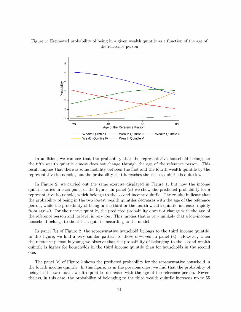
Figure 1: Estimated probability of being in a given wealth quintile as a function of the age ofthe reference person

0.1

.2.3

.4.5

.6P

roba

bili

ty

20 40 60 80Age of the Reference Person

Wealth Quintile I Wealth Quintile II Wealth Quintile III

Wealth Quintile IV Wealth Quintile V

In addition, we can see that the probability that the representative household belongs tothe fifth wealth quintile almost does not change through the age of the reference person. Thisresult implies that there is some mobility between the first and the fourth wealth quintile by therepresentative household, but the probability that it reaches the richest quintile is quite low.

In Figure 2, we carried out the same exercise displayed in Figure 1, but now the incomequintile varies in each panel of the figure. In panel (a) we show the predicted probability for arepresentative household, which belongs to the second income quintile. The results indicate thatthe probability of being in the two lowest wealth quintiles decreases with the age of the referenceperson, while the probability of being in the third or the fourth wealth quintile increases rapidlyfrom age 40. For the richest quintile, the predicted probability does not change with the age ofthe reference person and its level is very low. This implies that is very unlikely that a low-incomehousehold belongs to the richest quintile according to the model.

In panel (b) of Figure 2, the representative household belongs to the third income quintile.In this figure, we find a very similar pattern to those observed in panel (a). However, whenthe reference person is young we observe that the probability of belonging to the second wealthquintile is higher for households in the third income quintile than for households in the secondone.

The panel (c) of Figure 2 shows the predicted probability for the representative household inthe fourth income quintile. In this figure, as in the previous ones, we find that the probability ofbeing in the two lowest wealth quintiles decreases with the age of the reference person. Never-theless, in this case, the probability of belonging to the third wealth quintile increases up to 55

14

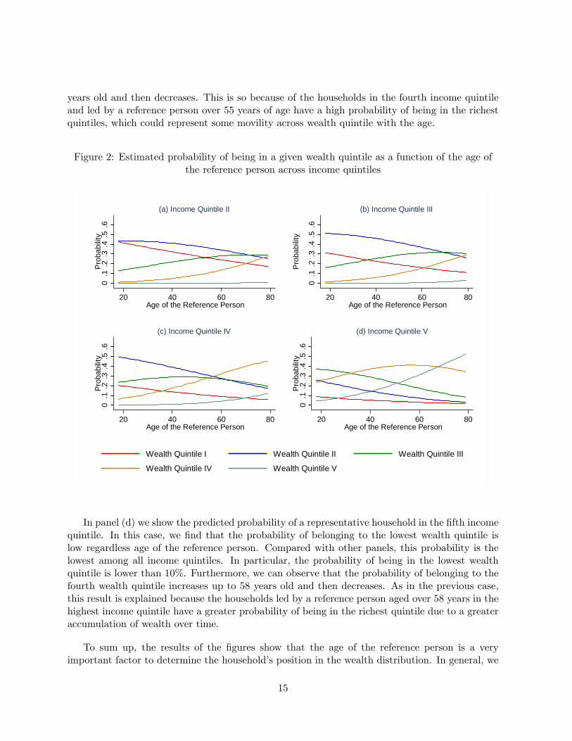
years old and then decreases. This is so because of the households in the fourth income quintileand led by a reference person over 55 years of age have a high probability of being in the richestquintiles, which could represent some movility across wealth quintile with the age.

Figure 2: Estimated probability of being in a given wealth quintile as a function of the age ofthe reference person across income quintiles

0.1

.2.3

.4.5

.6P

robabili

ty

20 40 60 80Age of the Reference Person

(a) Income Quintile II

0.1

.2.3

.4.5

.6

Pro

babili

ty20 40 60 80

Age of the Reference Person

(b) Income Quintile III

0.1

.2.3

.4.5

.6P

robabili

ty

20 40 60 80Age of the Reference Person

(c) Income Quintile IV

0.1

.2.3

.4.5

.6P

robabili

ty

20 40 60 80Age of the Reference Person

(d) Income Quintile V

Wealth Quintile I Wealth Quintile II Wealth Quintile III

Wealth Quintile IV Wealth Quintile V

In panel (d) we show the predicted probability of a representative household in the fifth incomequintile. In this case, we find that the probability of belonging to the lowest wealth quintile islow regardless age of the reference person. Compared with other panels, this probability is thelowest among all income quintiles. In particular, the probability of being in the lowest wealthquintile is lower than 10%. Furthermore, we can observe that the probability of belonging to thefourth wealth quintile increases up to 58 years old and then decreases. As in the previous case,this result is explained because the households led by a reference person aged over 58 years in thehighest income quintile have a greater probability of being in the richest quintile due to a greateraccumulation of wealth over time.

To sum up, the results of the figures show that the age of the reference person is a veryimportant factor to determine the household’s position in the wealth distribution. In general, we

15

find that as the age of the reference person rises, the probability of being in a higher wealth quintileincreases. We also note that while the household’s income increases, there is a low probability ofbelonging to the lowest wealth quintile. As we showed in Figure 2, the probability of being in thelowest wealth quintile goes from 30% in the second income quintile to 6% in the highest incomequintile for a household led by a person who is 30 years old. In addition, between the second andthe fourth income quintiles we see that there is some homogeneity in the patterns of the predictedprobability of belonging to a specific wealth quintile through the age of the reference person. Thisimplies that, even though the income has a significant effect in the probability of belonging toeach wealth quintile, these differences are not so important for these groups.

Finally, Table 7 replicates Table 2, but this time we use the wealth quintiles predicted for themodel to evaluate the relationship between income and wealth. The results show that even thoughthe income is a significant factor to explain the household’s position in the wealth distribution, therelationship between these two variables remains weak in the cross-section, even when we controlfor other variables. In fact, the diagonal of the matrix increases its weight, with the exception ofthe second quintile.24 This result shows that income only partially explains the wealth inequality.In fact, Leitner (2015) shows that only 11% of the wealth inequality is attributable to income.

Table 7: Joint distribution of income quintiles and model predicted values for wealth quintiles% of household in % of household predicted in quintiles of net wealthquintiles of income I II III IV V Total

I 30.8 13.9 34.5 19.4 1.4 100II 30.2 14.6 25.2 28.5 1.6 100III 14.6 37.9 22.7 22.4 2.5 100IV 2.5 35.2 13.8 37.1 11.3 100V 0.9 25.8 4.3 14.0 55.1 100

Source: Own calculations based on SHF 2014.

7 Conclusions

In this paper, we characterize the wealth distribution in the Chilean households and study thefactors that influence household position in the wealth distribution using the SHF 2014 collectedby Central Bank of Chile.

Our results show that net wealth is highly concentrated in Chilean households. In fact, therichest quintile accumulates 74% of total wealth. This level of concentration is similar to the levelobserved in Austria or Germany, which are the European countries with the most concentratedwealth distribution. In addition, we show that the Gini index for wealth in Chile is 0.74, whichimplies an unequal wealth distribution. This result is similar to the one observed in countries

24The result in the second quintile might be explained by the reallocation of household with zero wealth betweenthe first and the second wealth quintile.

16

such as Austria, Germany and the United States. The comparison with Latin American countriesis not posibble due to lack of information for other countries.

We also show that wealth is more unequal than income. This result is very common in theliterature related to wealth distribution. In fact, European countries and the United States showthe same relationship between income and wealth.

Regarding the factors that influence the household’s position in the wealth distribution, we findthat the age of the reference person and the household income increase the probability of being ina higher wealth quintile. We also show that the financing structure at the moment the householdbought its house is significant to explain the household’s position in the wealth distribution today.This result reflects that the past economic conditions of a household are useful to partially controlfor heterogeneous patterns of wealth accumulation.

Another important result is that housing-subsidy has a significant effect on the probability thathouseholds are above the first wealth quintile, but this variable affects negatively the probability ofa household being above the fourth wealth quintile. This implies that the public policies orientedto encourage housing tenure have had an important effect in wealth stocks of vulnerable Chileanhouseholds. This is a novel result in the literature because the analysis of wealth distribution indeveloping countries is quite limited.

In relation to the inheritance, the results show that receiving a property as an inheritanceincreases the probability of a household being in a better position in the wealth distributiontoday.

In terms of the relationship between wealth and income, we show that this is weak. Althoughincome has a significant effect on household position within the wealth distribution, we do notfind the position in the income distribution to be a good predictor of the position in the wealthdistribution.

Finally, we mention some challenges for future reasearch about wealth distribution. First, apanel dimension would be useful to study not only the current distribution, but also the het-erogeneous patterns in wealth accumulation. Second, the inlcusion of pension wealth would bebeneficial since this type of wealth is the most important asset for some households in Chile.

17

References

Arrondel, L., Roger, M., and Savignac, F. (2014) “Wealth and Income in the Euro Area: Het-erogeneity in Household’s Behaviours?”, Working Papers Series No 1709, European CentralBank.

Bauducco, S., and Castex, G. (2013) “The Wealth Distribution in Developing Economies: Com-paring the United States to Chile”, Banco Central de Chile, Documento de Trabajo No 702.

Brandolini, A., Cannari, L., D’Alessio, G., and Faiella, I. (2004) “Household Wealth Distributionin Italy in the 1990s”, Levy Economics Institute Working Paper, No. 414.

Bricker, J., Dettling, L., Henriques, A., Hsu, J., Moore, K., Sabelhaus, J., Thompson, J. andWindle, R. (2014) “Changes in U.S. Family Finances from 2010 to 2013: Evidence from theSurvey of Consumer Finances”, Federal Reserve Bulletin, Vol. 100, No. 4.

Brzozowski, M., Gervais, M., Klein, P., and Suzuki, M. (2010) “Consumption, Income and WealthInequality in Canada”, Review of Economic Dynamics, Vol 13(1): pp 52-75.

Caju, P. D. (2013) “Structure and Distribution of Household Wealth: an Analysis based onHFCS”, National Bank of Belgium Economic Review.

Carrol, C. D., Slacalek, J., and Tokuoka, K. (2014) “The Distribution of Wealth and the MPC:Implications of New European Data”, European Central Bank, Working Papers Series No1648.

Central Bank of Chile (2013) “Encuesta Financiera de Hogares: Metodología y Principales Re-sultados EFH 2011-12”, Banco Central de Chile.

Chau-Nan, C., Tien-Wang T., and Tong-Shieng, R. (1982) “The Gini Coeffi cient and NegativeIncome”, Oxford Economics Papers, Vol. 34 (3), pp. 473-478.

Cowell, F., Karagiannaki, E., and McKnight, A. (2012) “Accounting for Cross-Country Differencesin Wealth Inequality”, LWS Working Paper No 13.

Cox, P., Parrado, E., and Ruiz-Tagle, J. (2006) “The Distribution of Assets, Debt, and Incomeamong Chilean Households”, Banco Central de Chile, Documentos de Trabajo No 388.

Davies, J. B., Sandström , S., Shorrocks, A. and Wolff, E. N. (2011) “The Level and Distributionof Global Household Wealth”, The Economic Journal, Vol 121 (551), pp. 223—254.

Díaz-Giménez, J., Glover, A., and Ríos-Rull J.V. (2011) “Facts on the Distributions of Earn-ings, Income, and Wealth in the United States: 2007 Update”, Federal Reserve Bank ofMinneapolis Quarterly Review, Vol 34(1): pp. 2-31.

Encuesta Financiera de Hogares (2015a) “Encuesta Financiera de Hogares 2014: Cuestionario”,Banco Central de Chile.

Encuesta Financiera de Hogares (2015b) “Encuesta Financiera de Hogares 2014: PrincipalesResultados”, Banco Central de Chile.

18

Eurosystem Household Finance and Consumption Network (2013) “The Eurosystem HouseholdFinance and Consumption Survey: Methodological Report for the First Wave”, ECB Statis-tical Paper, Series, No 1.

Eckerstorfer, P., Halak, J., Kapeller, J., Schütz, B., and Springholz, F. (2015) “Correcting for theMissing Rich: An Application to Wealth Survey Data”, The Review of Income and Wealth,DOI: 10.1111/roiw.12188.

Fessler, P., and Schürz, M. (2015) “Private Wealth across European Countries: The role of Income,Inheritance and the Welfare State”, Working Papers Series No 1847, European Central Bank.

Greene, W., and Hensher, D. (2010) “Modelling Ordered Choices”, Cambridge Books, CambridgeUniversity Press.

Jantti, M., Sierminska, E., and Smeeding T. (2008) “The Joint Distribution of Household Incomeand Wealth: Evidence from the Luxembourg Wealth Study”, OECD Social, Employmentand Migration Working Paper No 65.

Kennickell, A. (1998) “Multiple Imputation in the Survey of Consumer Finances”, Proceedingsof the Section on Business and Economic Statistics, 1998 Annual Meetings of the AmericanStatistical Association.

Kennickell, A. (2003) “A Rolling Tide: Changes in the Distribution of Wealth in the US, 1989-2001”, paper presented at the Levy Institute Conference on International Perspectives onHousehold Wealth, October 2003.

Kennickell, A.B., and Woodburn, R. L. (1997) “Consistent Weight Design for the 1989, 1992, and1995 SCF’s, and the Distribution of Wealth”, Review of Income and Wealth, Vol 25 (2), pp.193-215.

Kontbay-Busun, A., and Peichl, A. (2015) “Multidimensional Affl uence in Income and Wealth inthe Eurozone: A Cross-Country Comparison Using HFCS”, IZA Discussion Paper No 9139,June 2015.

Leitner, S. (2015) “Drivers of Wealth Inequality in Euro Area Countries”, wiiw Working PaperNo 122, The Vienna Institute for International Economic Studies.

Martínez, F., and Uribe, F. (2017) “Distribución de Riqueza no Previsional de los HogaresChilenos", Banco Central de Chile, Documento de Trabajo.

Mathä, T., Porpiglia, A., and Ziegelmeyer, M. (2014) “Household Wealth in the Euro Area:The Importance of Intergenerational Transfers, Homeownership and House Price Dynamics”,Working Paper Series No. 1690, European Central Bank.

OECD (2013) “OECD Guidelines for Micro Statistics on Household Wealth”, OECD Publishing.

OECD (2015) “In It Together: Why less Inequality Benefits All?”, OCDE Publishing, Paris.

Pfeffer, F., and Griffi n, J. (2015) “Determinants of Wealth Fluctuations”, Technical Series PaperNo15-01, PSID.

19

Piketty, T. (2014) “Capital in the Twenty-First Century”, Havard University Press.

Rao, J.N.K., and Wu, C.F.J. (1988) “Resampling Inference with Complex Survey Data”, Journalof American Statistical Association, Vol. 83 (401), pp. 231-241.

Rubin, D. B. (1987) “Multiple Imputation for Nonresponse in Surveys”, John Wiley and Sons.New York.

Sierminska, E., and Medgyesi, M. (2013) “The Distribution of Wealth between Households”,European Commission, Research Note 11/2013.

Stiglitz, J. E., Sen, A. and Fitoussi, J. P. (2009) “Report by the Commission on the Measure-ment of Economic Performance and Social Progress”, Commission on the Measurement ofEconomic Performance and Social Progress.

Vermeulen, P. (2014) "How Fat is the Top tail of the wealth Distribution?", European CentralBank, Working Papers Series No 1692.

Williams, R. (2006) “Generalized Ordered Logit/Partial Proportional Odds Models for OrdinalDependent Variables”, The Stata Journal, Vol. 6, pp: 58-82.

Wolff, E. N. (2010) “Recent Trends in Household Wealth in the United States: Rising Debt andthe Middle-Class Squeeze - an Update to 2007”, Levy Economics Institute of Board College,Working Paper No 589.

20

Appendix

A Household reference person

The household reference person was selected according to the criteria presented in the 2011 Cam-berra Group Handbook on Household Income Statistics.25

To identify the household reference person, the following criteria were applied sequentially toall household members, in order listed below, until a single person was identified:

1. One of the partners in a registered or de facto marriage, with children aged 0-17 years.

2. One of the partners in a registered or de facto marriage, without children aged 0-17 years.

3. A single parent with children aged 0-17 years.

4. The person with the highest income.

5. The oldest person.

For example, in the case of three persons all aged 18 years or more and none of them ina registered or de facto marriage, the person with the highest income would be selected as thereference person. If two of them were married, the partner with the highest income would beselected as the reference person. If the income of the partners were equal, the oldest partnerwould be selected as the reference person.

For households where it was not possible to identify a reference person according to the abovecriteria, we adopted an additional criterion:

6. Person self-reported as head of household.

25United Nations (UN).

21

Documentos de Trabajo

Banco Central de Chile

NÚMEROS ANTERIORES

La serie de Documentos de Trabajo en versión PDF

puede obtenerse gratis en la dirección electrónica:

www.bcentral.cl/esp/estpub/estudios/dtbc.

Existe la posibilidad de solicitar una copia impresa

con un costo de Ch$500 si es dentro de Chile y

US$12 si es fuera de Chile. Las solicitudes se

pueden hacer por fax: +56 2 26702231 o a través del

correo electrónico: bcch@bcentral.cl.

Working Papers

Central Bank of Chile

PAST ISSUES

Working Papers in PDF format can be downloaded

free of charge from:

www.bcentral.cl/eng/stdpub/studies/workingpaper.

Printed versions can be ordered individually for

US$12 per copy (for order inside Chile the charge

is Ch$500.) Orders can be placed by fax: +56 2

26702231 or by email: bcch@bcentral.cl.

DTBC – 826

Revisiting the Exchange Rate Pass Through: A General Equilibrium Perspective

Mariana García-Schmidt y Javier García-Cicco

DTBC – 825

An Econometric Analysis on Survey-data-based Anchoring of Inflation Expectations

in Chile

Carlos A. Medel

DTBC – 824

Can Economic Perception Surveys Improve Macroeconomic Forecasting in Chile?

Nicolas Chanut, Mario Marcel y Carlos Medel

DTBC – 823

Characterization of the Chilean Financial Cycle, Early Warning Indicators and

Implications for Macro-Prudential Policies

Juan Francisco Martínez y Daniel Oda

DTBC – 822

Taxonomy of Chilean Financial Fragility Periods from 1975 Juan Francisco Martínez, José Miguel Matus y Daniel Oda

DTBC – 821

Pension Funds and the Yield Curve: the role of Preference for Maturity Rodrigo Alfaro y Mauricio Calani

DTBC – 820

Credit Guarantees and New Bank Relationships

William Mullins y Patricio Toro

DTBC – 819

Asymmetric monetary policy responses and the effects of a rise in the inflation target

Benjamín García

DTBC – 818

Medida de Aversión al Riesgo Mediante Volatilidades Implícitas y Realizadas

Nicolás Álvarez, Antonio Fernandois y Andrés Sagner

DTBC – 817

Monetary Policy Effects on the Chilean Stock Market: An Automated Content

Approach Mario González y Raúl Tadle

DTBC – 816

Institutional Quality and Sovereign Flows

David Moreno

DTBC – 815

Desarrollo del Crowdfunding en Chile

Iván Abarca

DTBC – 814

Expectativas Financieras y Tasas Forward en Chile

Rodrigo Alfaro, Antonio Fernandois y Andrés Sagner

DTBC – 813

Identifying Complex Core-Periphery Structures in the Interbank Market

José Gabriel Carreño y Rodrigo Cifuentes

DTBC – 812

Labor Market Flows: Evidence for Chile Using Micro Data from Administrative Tax

Records Elías Albagli, Alejandra Chovar, Emiliano Luttini, Carlos Madeira, Alberto Naudon,

Matías Tapia

DOCUMENTOS DE TRABAJO • Septiembre 2018