UNIVERSIDAD COMPLUTENSE DE MADRID FACULTAD DE CIENCIAS MATEMÁTICAS DEPARTAMENTO DE GEOMETRÍA Y TOPOLOGÍA

TESIS DOCTORAL

CONEXIONES DE AMBROSE-SINGER Y ESTRUCTURAS HOMOGÉNEAS EN VARIEDADES PSEUDO-RIEMANNIANAS

AMBROSE-SINGER CONNECTIONS AND HOMOGENEOUS STRUCTURES ON PSEUDO-RIEMANNIAN MANIFOLDS

MEMORIA PARA OPTAR AL GRADO DE DOCTOR

PRESENTADA POR

Ignacio Luján Fernández

Director

Marco Castrillón López

Madrid, 2014 © Ignacio Luján Fernández, 2014

CONEXIONES DE AMBROSE-SINGER YESTRUCTURAS HOMOGENEAS EN

VARIEDADES PSEUDO-RIEMANNIANAS

AMBROSE-SINGER CONNECTIONS ANDHOMOGENEOUS STRUCTURES ON

PSEUDO-RIEMANNIAN MANIFOLDS

Memoria presentada para optar al grado deDoctor en Ciencias Matematicas por

Ignacio Lujan Fernandez

Dirigida por

Dr. Marco Castrillon Lopez

Departamento de Geometrıa y TopologıaFacultad de Ciencias Matematicas

Universidad Complutense de Madrid

A mis padres

“At ubi materia, ibi Geometria.”“Where there is matter, there is geometry”

Johannes Kepler

Agradecimientos

Este trabajo ha sido financiado por una beca FPU del Ministerio de Educacion (2010-2014) y por el proyecto de investigacion MTM-2011-22528 del Ministerio de Ciencia eInnovacion.

En primer lugar quiero dar las gracias a mi director de tesis Marco Castrillon Lopez.Siempre estare en deuda con el, no solo por su incalculable guıa y ayuda duranteestos anos, sino sobre todo por haberme contagiado su entusiasmo y placer por lasMatematicas. De el he aprendido 2ℵ0 cosas, y ninguna de ellas ha sido trivial.

Agradezco ası mismo al Departamento de Geometrıa y Topologıa haberme acogidodurante el desarrollo de este trabajo. Este agradecimiento se extiende a toda la Facultadde Matematicas de la UCM, pero en especial a todos aquellos profesores que con sudesinteresada dedicacion mantienen vivo el programa de Doctorado.

I would also like to thank Andrew Swann and Anna Fino for their hospitality dur-ing my stays at Aahrus and Torino, and for such enlightening discussions on severaltopics of Differential Geometry. It was a great pleasure to learn and work with them.Tambien estoy en deuda con Pedro Martınez Gadea, que siempre saco tiempo paravaliosos consejos, sugerencias, y alguna que otra correccion.

Quiero agradecer todos los buenos ratos a los doctorandos de matematicas: Carlos,Fonsi, Javi, Luis, Andrea, Alvarito, Quesada, Diego, Espe, Ali, Laura, Simone, Giovanni,Silvia, Manu y Hector. Desde los seminarios en los sofas de Tino’s donde descubrimosque toda matriz en C es diagonalizable (bueno, salvo quiza una o dos), hasta el agujerode gusano donde el profesor Jean Paul imparte sus cursos de astrofısica. Con ellos hecomprendido que compartir las Matematicas es elevarlas al cuadrado.

No puedo continuar sin hacer mencion a mis amigos, los Pilaristas: Rafa, Chino,Palao, Pena, Choco, Prada, Pollo, Mariano, Mallol, Loren, Douglas y Fafa. Siempre mehabeis hecho las preguntas mas difıciles: ¿De que va tu tesis? ¿Y eso para que sirve? ¿Ysolo usas papel y boli? ¿Por que no te metes a un banco y empiezas a forrarte de pasta?Y aunque yo responda torpemente, nunca os habeis cansado de preguntar. Gracias porcreer siempre en mı y aguantar alguna “chapa” matematica mas de la cuenta. No seme dan muy bien los numeros, pero creo que son ya 21 anitos juntos.

Sin lugar a dudas este trabajo nunca habrıa sido posible sin mi familia, en especialmis padres y mis hermanos. A ellos les agradezco el apoyo y aliento que he recibido paraalcanzar esta meta. Si bien creo que nunca conseguı que entendiesen en que consiste estode la Geometrıa Diferencial, espero que sı comprendan que gracias a ellos he conseguidorealizar un sueno. Ellos supieron ver antes que nadie cual era mi camino. Quiero dar lasgracias tambien de manera especial a mis abuelos Manolo, Amarfil, Enrique y Aurora,y mis tıos Amador y Paca. Porque su fe ciega siempre me ayudo a apuntar alto.

Por ultimo, un lugar especial en estos agradecimientos le pertenece por derechopropio a Marta. Por guıarme, por su incansable animo, y por aguantarme todos estosanos (si detras de todo hombre hay una gran mujer, detras de este doctorando hay unagran mujer con infinita paciencia), pero sobre todo por sacar siempre la mejor versionde mı mismo. Ese merito es todo suyo. A su lado ningun problema parecio nuncademasiado difıcil.

Contents

Summary i

Resumen vii

1 Preliminaries 11.1 Principal bundles and connections . . . . . . . . . . . . . . . . . . . . . 1

1.1.1 Principal bundles . . . . . . . . . . . . . . . . . . . . . . . . . . . 11.1.2 Connections on principal bundles . . . . . . . . . . . . . . . . . . 21.1.3 Holonomy . . . . . . . . . . . . . . . . . . . . . . . . . . . . . . . 5

1.2 Pseudo-Riemannian connections, G-structures, and Berger’s Theorem . 71.2.1 Pseudo-Riemannian connections and G-structures . . . . . . . . 71.2.2 Berger’s Theorem . . . . . . . . . . . . . . . . . . . . . . . . . . 91.2.3 Geometric description of some G-structures . . . . . . . . . . . . 11

1.3 Homogeneous spaces and the canonical connection . . . . . . . . . . . . 23

2 Ambrose-Singer connections and homogeneous spaces 292.1 Symmetric spaces and Cartan’s Theorem . . . . . . . . . . . . . . . . . 292.2 Ambrose-Singer and Kiricenko’s Theorems . . . . . . . . . . . . . . . . . 302.3 Homogeneous structures . . . . . . . . . . . . . . . . . . . . . . . . . . . 35

3 Locally homogeneous pseudo-Riemannian manifolds 393.1 Reductive locally homogeneous pseudo-Riemannian manifolds . . . . . . 39

3.1.1 Locally homogeneous pseudo-Riemannian manifolds with invari-ant geometric structures . . . . . . . . . . . . . . . . . . . . . . . 46

3.2 Strongly reductive locally homogeneous pseudo-Riemannian manifolds . 483.3 Reconstruction of strongly reductive locally homogeneous spaces . . . . 533.4 Examples and the reductivity condition . . . . . . . . . . . . . . . . . . 58

4 Classification of homogeneous structures 634.1 General procedure . . . . . . . . . . . . . . . . . . . . . . . . . . . . . . 634.2 Some classifications . . . . . . . . . . . . . . . . . . . . . . . . . . . . . . 65

4.2.1 Homogeneous pseudo-Riemannian structures . . . . . . . . . . . 654.2.2 Homogeneous pseudo-Kahler structures . . . . . . . . . . . . . . 664.2.3 Homogeneous para-Kahler structures . . . . . . . . . . . . . . . . 684.2.4 Homogeneous pseudo-quaternion Kahler structures . . . . . . . . 704.2.5 Homogeneous para-quaternion Kahler structures . . . . . . . . . 734.2.6 Homogeneous Sasakian and cosymplectic structures . . . . . . . 77

5 Homogeneous ε-Kahler structures of linear type 815.1 The non-degenerate case . . . . . . . . . . . . . . . . . . . . . . . . . . . 815.2 The degenerate case . . . . . . . . . . . . . . . . . . . . . . . . . . . . . 84

5.2.1 Local form of the metrics . . . . . . . . . . . . . . . . . . . . . . 885.3 Infinitesimal models, homogeneous models and completeness . . . . . . . 95

5.3.1 The non-degenerate para-Kahler case . . . . . . . . . . . . . . . 97

5.3.2 The non-degenerate pseudo-Kahler case . . . . . . . . . . . . . . 995.3.3 The degenerate case with λ = − ε

2 . . . . . . . . . . . . . . . . . 1005.3.4 The degenerate case with λ = 0 . . . . . . . . . . . . . . . . . . . 102

5.4 Relation with homogeneous plane waves . . . . . . . . . . . . . . . . . . 103

6 Homogeneous ε-quaternion Kahler structures of linear type 1076.1 Characterizing homogeneous ε-quaternion Kahler structures of linear type 1086.2 Infinitesimal models, homogeneous models and completeness . . . . . . . 111

6.2.1 The para-quaternion Kahler case . . . . . . . . . . . . . . . . . . 1116.2.2 The pseudo-quaternion Kahler case . . . . . . . . . . . . . . . . . 114

7 Reduction of homogeneous structures 1177.1 Reduction by a normal subgroup of isometries . . . . . . . . . . . . . . . 118

7.1.1 The space of tensors reducing to a given tensor . . . . . . . . . . 1217.2 Reduction in a principal bundle . . . . . . . . . . . . . . . . . . . . . . . 122

7.2.1 Examples . . . . . . . . . . . . . . . . . . . . . . . . . . . . . . . 1277.3 Application to cosymplectic and Sasakian homogeneous structures of lin-

ear type . . . . . . . . . . . . . . . . . . . . . . . . . . . . . . . . . . . . 132

8 Appendix: Computations concerning formula (5.17) 137

Summary

Ambrose-Singer connections and homogeneous structures on pseudo-Riemannianmanifolds.

Conexiones de Ambrose-Singer y estructuras homogeneas en variedadespseudo-Riemannianas.

Introduction

Homogeneous and locally homogeneous spaces enjoy a large group of internal symme-tries. For that reason they constitute a distinguished class of spaces on which the studyof pseudo-Riemannian geometry is especially rich and varied. This kind of spaces havebeen extensively studied by means of many different methods and techniques. One dif-ficulty arising is that the same pseudo-Riemannian manifold (M, g) can admit severaldifferent descriptions as a coset space G/H. It is surprising how little is known aboutthis problem for many well-known spaces. One of the most fruitful approaches was at-tempted by Ambrose and Singer, who in 1958 [4] extended Cartan’s characterization ofsymmetric spaces. They characterized connected, simply-connected and complete ho-mogeneous Riemannian manifolds as Riemannian manifolds (M, g) admitting a linear

connection ∇ satisfying

∇g = 0, ∇R = 0, ∇S = 0,

where S = ∇ − ∇, ∇ is the Levi-Civita connection of g, and R is the curvature ofg. These equations would become later known as Ambrose-Singer equations, and con-nections satisfying them as Ambrose-Singer connections. The previous result not onlycharacterizes homogeneous spaces in a “nice” way, but also introduces a new tool forstudying the geometry of this kind of manifolds, namely the Ambrose-Singer connec-tion ∇ and the so called homogeneous structure tensor S (or homogeneous structure forshort). Since their introduction, these objects have proved to be very useful, probablydue to the combination of their geometric and algebraic natures. The first results in thisdirection were obtained by Tricerri and Vanhecke in [60], where the algebraic nature ofS allowed the authors to achieved a classification of homogeneous Riemannian structuretensors into eight different classes using only algebraic arguments and a representationtheoretical approach. They further identified two of those classes with spaces of con-stant sectional curvature and naturally reductive homogeneous spaces respectively. Thistheory was extended to locally homogeneous Riemannian spaces by several authors (seefor instance [40] and [59]). In this setting, the canonical Ambrose-Singer connectionconstructed by Kowalski in [40] becomes the central axis around which the theory isbuilt.

Ambrose-Singer Theorem was generalized by Kiricenko to the case when the Rie-mannian manifold (M, g) is endowed with a geometric structure defined by a set oftensor fields P1, . . . , Pn. In that case, one have to add the conditions

∇P1 = 0, . . . , ∇Pn = 0

to Ambrose-Singer equations. Similar classifications of homogeneous Riemannian struc-tures to that provided by Tricerri and Vanhecke were obtained by several authors inthe presence of different geometric structures, and in [26], the classification for all the

i

ii

holonomies appearing in Berger’s list is achieved by a representation theoretical ap-proach. In many cases (such as Kahler, hyper-Kahler, quaternion Kahler, G2 or Spin(7))these classifications contain a class consisting of sections of a bundle whose rank growslinearly with the dimension of the manifold. For that reason homogeneous structuresbelonging to these classes are called of linear type. The corresponding tensor fields Sare defined by a set of vector fields satisfying a system of PDE’s equivalent to Ambrose-Singer equations. The importance of this kind of structures relies on the fact that in thepurely Riemannian case so as in the case of Kahler and quaternion Kahler manifolds,homogeneous structures of linear type characterize spaces of negative constant sectional(resp. holomorphic sectional, quaternionic sectional) curvature (see [60], [29] and [16]).

In [31] Ambrose-Singer Theorem is adapted to metrics with arbitrary signature.As it is well known, every homogeneous Riemannian manifold is reductive, but this isno longer true if the metric is not definite. This way, the pseudo-Riemannian versionof Ambrose-Singer Theorem states that the existence of an Ambrose-Singer connec-tion characterizes reductive homogeneous pseudo-Riemannian manifolds under suitabletopological conditions.

Some of the techniques used in the Riemannian case have also been adapted to met-rics with signatures in order to obtain classifications of homogeneous pseudo-Riemannianstructures, both in the purely pseudo-Riemannian case and in the presence of a geo-metric structure (see for instance [31], [30] and [8]). In this situation we also havethat in many cases (such as pseudo-Kahler, para-Kahler, pseudo-hyper-Kahler, para-hyper-Kahler, pseudo-quaternion Kahler, para-quaternion Kahler, G∗2(2) or Spin(4, 3))there is a class, also called of linear type, consisting of sections of a bundle whose rankgrows linearly with the dimension of the manifold. When metrics with signature arestudied, the causal character of the vector fields defining the homogeneous structuretensor needs to be taken into account. In the purely pseudo-Riemannian case, non-degenerate homogeneous structures of linear type (i.e. given by a non null vector field)characterize spaces of constant sectional curvature [31]. On the other hand, degeneratehomogeneous structures of linear type (i.e. given by a null vector field) characterizesingular scale-invariant homogeneous plane waves [46]. Furthermore, in [45] it is shownthat homogeneous structures in the composed class S1 +S3 are related to a larger classof singular homogeneous plane waves. It is worth pointing out that very less is knownabout homogeneous spaces with holonomy G∗2(2) or Spin(4, 3). It is even very difficult tofind non-flat examples in the literature, and most of them have low dimensional holon-omy. Concerning this situation, new examples of Lie groups with left-invariant metricswith full holonomy G∗2(2) have been recently obtained in [27].

Objectives

The present dissertation has three main objectives. In the first place, we want to extendAmbrose-Singer Theorem to locally homogeneous pseudo-Riemannian manifolds. Theadaptation of the theory is not as straightforward as in the Riemannian case, and newconcepts need to be developed. In addition we will like to explore how the constructionof the canonical connection made by Kowalski fits in the pseudo-Riemannian setting,and in particular if the reconstruction of a locally homogeneous space from the cur-vature and its covariant derivatives up to finite order still holds. Secondly, we wouldlike to characterize homogeneous structures of linear type in the pseudo-Kahler, para-Kahler, pseudo-quaternion Kahler and para-quaternion Kahler cases. As it happenedin the purely pseudo-Riemannian case, the causal character of the vector fields definingthe homogeneous structure opens room for new objects and scenarios, which do notexist in the Riemannian realm. Finally, we are interested in studying the behavior ofhomogeneous structures within the framework of reduction under a group of isometries.Reduction procedures are widely use in many settings of differential geometry in order

iii

to construct new objects or to obtain new information from known cases. This way, areduction scheme for homogeneous structures can be very convenient for the study ofhomogeneity.

Outline and results

In Chapter 1 we settle the foundations for subsequent chapters. More precisely, webriefly introduce the theory of principal bundles and connections. We also define theholonomy of a connection and present the most relevant results. This concept will becentral throughout the rest of the manuscript. We then apply this theory to pseudo-Riemannian manifolds and G-structures. After stating Berger’s Theorem, we describesome basic features of the geometric structures we will deal with in Chapters 5, 6 and7. We finally introduce the basics about homogeneous spaces and define the canonicalconnection associated to a reductive homogeneous space. This is the first and mostrepresentative example of Ambrose-Singer connection.

In Chapter 2 we state Ambrose-Singer Theorem, which is the starting point of thetheory of Ambrose-Singer connections and of the present dissertation. We first contex-tualize this result relating it with Cartan’s characterization of symmetric spaces. Wealso present Kiricenko’s Theorem, which extends Ambrose-Singer Theorem to the casewhen the manifold is endowed with an extra geometric structure. Since the author ofthis thesis has not found any proof of Kiricenko’s Theorem in the literature, an originalproof is given. We end this chapter defining the homogeneous structure tensor associatedto an Ambrose-Singer connection. We introduce the corresponding infinitesimal model,Nomizu construction and transvection algebra, and discuss some of their properties.

In Chapter 3 we develop the theory of Ambrose-Singer connections on locally homo-geneous pseudo-Riemannian manifolds. We prove that a locally homogeneous pseudo-Riemannian manifold admits an Ambrose-Singer connection if it satisfies an algebraiccondition concerning the set of local Killing vector fields (Theorem 3.1.9). In analogywith the global case, we call this condition reductive. Conversely, we show that a pseudo-Riemannian manifold admitting an Ambrose-Singer connection is locally homogeneousand reductive (Theorem 3.1.10). As it is well known, different Lie (pseudo-)groups canact transitively on the same (locally) homogeneous manifold. We will see that the notionof reductivity is a property concerning the action of a certain Lie (pseudo-)group ratherthan a property of the manifold itself. Note that this follows the spirit of F. Klein’sErlangen Programm, pointing out that different actions on the same manifold mighthave a very different nature. Several examples will explore the possible scenarios. Wewill further extend the previous results to manifolds endowed with an extra geometricstructure (Theorems 3.1.16 and 3.1.17). Following the work of Kowalski in the Rie-mannian case [40], a new condition, which we will call strong reductivity, will naturallyappear. We prove that strongly reductive (locally) homogeneous pseudo-Riemannianmanifolds admit a very special Ambrose-Singer connection analogous to the canonicalconnection constructed by Kowalski in the Riemannian case (Theorem 3.2.8). Unlikethe reductivity condition, this new condition is indeed a property of the manifold itselfand not of the action of any Lie (pseudo-)group. We study some properties of stronglyreductive locally homogeneous pseudo-Riemannian manifolds, and in particular we see(Theorem 3.3.2) that they can be recovered from the curvature and its covariant deriva-tives up to finite order at some point (recall that this property is enjoyed by all locallyhomogeneous Riemannain manifolds [49]).

In Chapter 4 we exploit the algebraic nature of homogeneous structures in order toobtain classification results. We first sketch a general procedure to classify homogeneousstructures with or without the presence of a geometric structure, and we then specifyit for the geometric structures and the holonomies appearing in Chapters 5, 6 and 7.We define the so called homogeneous structures of linear type, which are homogeneous

iv

structures characterized by a set of vector fields. These will be the main object of studyin Chapters 5 and 6. All the classifications obtained in this chapter were previously ob-tained by several authors, except for the para-quaternion Kahler, pseudo-hyper-Kahlerand para-hyper-Kahler cases which are original.

In Chapter 5 we study homogeneous pseudo-Kahler and para-Kahler structures oflinear type. On the one hand we prove that pseudo-Kahler and para-Kahler manifoldsadmitting a non-degenerate homogeneous pseudo-Kahler and para-Kahler structures oflinear type respectively (see Definitions 4.2.6 and 4.2.9) have constant holomorphic andpara-holomorphic sectional curvature respectively (Theorem 5.1.2). We moreover showthat the corresponding complex and para-complex space forms only admits these kind ofstructures locally, unless the metric is definite (Theorems 5.3.1). On the other hand weobtain the holonomy (Propositions 5.2.2 and 5.2.4) and the local form of pseudo-Kahlerand para-Kahler manifolds admitting a degenerate homogeneous pseudo-Kahler andpara-Kahler structures of linear type respectively (Propositions 5.2.5 and 5.2.6), focusingon the singular nature of the metrics. We compute the associated infinitesimal modeland transvection algebra for both cases, and study the completeness of the correspondinghomogeneous model (Theorem 5.3.2). We finally exhibit the relation between degeneratestructures and certain kind of homogeneous plane waves. Some of the results containedin this chapter, namely those referring to strongly degenerate structures, were publishedin [18].

In Chapter 6 we study homogeneous pseudo-quaternion Kahler and para-quaternionKahler structures of linear type. On the one hand we prove that pseudo-quaternionKahler and para-quaternion Kahler manifolds admitting a non-degenerate homoge-neous pseudo-quaternion Kahler and para-quaternion Kahler structures of linear typerespectively (see Definitions 4.2.12 and 4.2.15) have constant quaternionic and para-quaternionic sectional curvature respectively (Theorem 6.1.1). We moreover show thatthe corresponding quaternion and para-quaternion space forms only admits these kindof structures locally, unless the metric is definite (Theorem 6.2.1). On the other hand weshow that pseudo-quaternion Kahler and para-quaternion Kahler manifolds admitting adegenerate homogeneous pseudo-quaternion Kahler and para-quaternion Kahler struc-tures of linear type are flat (Theorem 6.1.1). We compute the associated infinitesimalmodel and transvection algebra for the non-degenerate case, and study the completenessof the corresponding homogeneous model (Theorem 6.2.2).

Finally, in Chapter 7 we study homogeneous structures within the framework ofreduction under a group H of isometries. In a first result, H is a normal subgroup ofthe group of symmetries associated to a homogeneous structure S defined on a globallyhomogeneous space. In this case S can be reduced to a homogeneous structure inthe space of orbits under the action of H (Theorem 7.1.4). In a second result westudy under which conditions a homogeneous structure S defined on the total spaceof a principal bundle π : (M, g) → (M, g) reduces to a homogeneous structure on thebase space (M, g). The answer (Theorem 7.2.1) involves an additional condition on theso called mechanical connection of the principal bundle which resembles to the extraequation appearing in Kiricenko’s Theorem. The behavior of the classes of homogeneoustensors are also investigated when reduction is performed (Proposition 7.2.3). It turnsout that the geometry of the fibres is involved in the preservation of some of them(Proposition 7.2.4). Some classical examples illustrate the theory. Finally, the reductionprocedure is applied to fiberings of almost contact manifolds over almost Hermitianmanifolds. If the homogeneous structure is moreover cosymplectic or Sasakian, theobtained reduced homogeneous structure is pseudo-Kahler. We will use this result toobtain some properties of homogeneous cosymplectic and Sasakian structures of lineartype (Propositions 7.3.8 and 7.3.10). The contents of this chapter are included in [19].

v

Conclusions

Regarding the first objective, we have been able to extend Ambrose-Singer Theorem andthe theory of Ambrose-Singer connections to locally homogeneous pseudo-Riemannianmanifolds. We have seen that the arguments used in the Riemannian case do notdirectly hold in this setting, and a deeper inspection has led to new concepts as reduc-tive and strong reductive locally homogeneous pseudo-Riemannian manifolds. Thesenew concepts reveal themselves as necessary not only in order to develop the theoryof Ambrose-Singer connections, but to extend the results from the Riemannian settingto metrics of arbitrary signature. It is very interesting how the transition from theRiemannian setting to the case of metrics with signature usually gives some perspec-tive and reveals the Riemannian case as a very special situation. Regarding this, it isworth pointing out that very less is known about non-reductive homogeneous pseudo-Riemannian manifolds (see for example [25]). I believe that Chapter 3 sheds some lightto this problem.

Concerning the second objective, we have been able to characterize the class of ho-mogeneous structures of linear type in the case of pseudo-Kahler, para-Kahler, pseudo-quaternion Kahler and para-quaternion Kahler geometries. It is very interesting howthe causal character of the set of vector field defining the homogeneous structures sep-arates two different worlds. On the one hand, non-degenerates structures give resultswhich resemble to the Riemannian case, namely they characterize manifolds of con-stant (para-)holomorphic and (para-)quaternionic sectional curvature. On the otherhand, degenerate structures have no Riemannian counterpart, so that genuine pseudo-Riemannian situations appear. More precisely, in the pseudo-Kahler and para-Kahlercases, these kind of homogeneous structures characterize manifolds whose underlyinggeometry can be interpreted as a (para-)complex generalization of the geometry ofhomogeneous plane waves. In the pseudo-quaternion and para-quaternion cases thecondition ∇R = 0 in Ambrose-Singer equations becomes too strong, and the manifoldis forced to be flat, suggesting that the notion of homogeneous plane wave cannot beextended to geometries of quaternionic type. Another remarkable feature about bothdegenerate and non-degenerate structures, is that completeness issues naturally arise.More precisely, besides the fact that the underlying geometry of degenerate structuresseems to be singular (in a cosmological sense), all homogeneous models associated tothese homogeneous structures are necessarily incomplete. The origin of these complete-ness issues seems fuzzy at this moment and could be an interesting topic of research inthe future.

Finally, the third objective has been accomplished providing a good reduction schemefor homogeneous structures. It is noteworthy the role played by the geometry of theprincipal fiber bundle and the Kiricenko condition on the mechanical connection involvedin the reduction scheme. It is also worth stressing how the geometry of the fibers areinvolved in the preservation of some classes of homogeneous structures. As desired,this results have allowed us to study new objects from known ones. More precisely, wehave been able to study some properties of homogeneous cosymplectic and Sasakianstructures of linear type making use of the reduction procedure and our knowledge ofhomogeneous pseudo-Kahler structures of linear type. Many problems still remain openfor the future. In the first place, an inverse procedure would be of great value, namelywe would like to find suitable conditions to define homogeneous structures on the totalspace of a principal bundle from homogeneous structures defined in the base space.Secondly, a complete study of homogeneous cosymplectic and Sasakian structures oflinear type remains to be done, since we have only deal with invariant structures. Theproperties we have obtained in this part of the thesis would be a head start for thispurpose.

The works derived from topics of this thesis appear in [18], [19], [20], [27], [41], and[42].

Resumen

Conexiones de Ambrose-Singer y estructuras homogeneas en variedadespseudo-Riemannianas / Ambrose-Singer connections and homogeneous structures on

pseudo-Riemannian manifolds.

Introduccion

Los espacios homogeneos y localmente homogeneos poseen un gran grupo de simetrıasinternas. Por esta razon constituyen una clase distinguida de espacios en los cualesel estudio de la geometrıa pseudo-Riemanniana es especialmente rica y variada. Estetipo de espacios han sido extensamente estudiados por medio de diferentes metodosy tecnicas. Una de las dificultades que aparecen es que la misma variedad pseudo-Riemanniana (M, g) puede admitir diferentes descripciones como espacio cociente G/H.Es sorprendente lo poco que se sabe acerca de este problema incluso para espacios bienconocidos. Una de las aproximaciones mas fructıferas fue desarrollada por Ambrose ySinger, quienes en 1958 [4] extendieron la caracterizacion de espacios simetricos dada porCartan. Estos autores caracterizaron los espacios homogeneos Riemannianos conexos,simplemente conexos y completos como aquellos que admiten una conexion lineal ∇ quesatisface

∇g = 0, ∇R = 0, ∇S = 0,

donde S = ∇−∇, ∇ es la conexion de Levi-Civita de g, y R es la curvatura de g. Estasecuaciones pasaron a llamarse ecuaciones de Ambrose-Singer, y las conexiones satis-faciendolas pasaron a llamarse conexiones de Ambrose-Singer. El resultado anterior nosolo caracteriza los espacios homogeneos de una manera “agradable”, sino que ademasintroduce una nueva herramienta para su estudio: las conexiones de Ambrose-Singer yel llamado tensor de estructura homogenea S (o estructura homogenea para abreviar).Desde su introduccion, estos objetos han probado ser de gran utilidad, probablementedebido a la combinacion de sus naturalezas algebraica y geometrica. El primer resul-tado en esta direccion fue obtenido por Tricerri y Vanhecke en [60], donde la naturalezaalgebraica de S permitio a los autores dar una clasificacion de los tensores estructurahomogenea Riemannianos usando solamente argumentos algebraicos y Teorıa de Rep-resentacion. Mas aun, los autores identificaron dos de las clases con los espacios decurvatura seccional constante y los espacios naturalmente reductivos respectivamente.Esta teorıa fue extendida a espacios Riemannianos localmente homogeneos por variosautores (vease por ejemplo [40] y [59]). En este ambito, la conexion canonica construidapor Kowalski en [40] es el eje central alrededor del cual se articula la teorıa.

El Teorema de Ambrose-Singer fue generalizado por Kiricenko al caso en que lavariedad Riemanniana (M, g) estuviese dotada de una estructura geometrica definidapor un conjunto de campos tensoriales P1, . . . , Pn. En este caso tenemos que anadir lascondiciones ∇P1 = 0, . . . , ∇Pn = 0 a las ecuaciones de Ambrose-Singer. Desde entoncesvarios autores han obtenido clasificaciones similares a la dada por Tricerri y Vanheckeen presencia de una estructura geometrica, y en [26], se estudian las clasificacionespara todas las holonomıas Riemannianas en la lista de Berger por medio de Teorıade Representacion. En muchos casos (tales como Kahler, hiper-Kahler, cuaternionicoKahler, G2 o Spin(7)) estas clasificaciones contienen una clase que consiste en seccionesde un fibrado cuyo rango crece linealmente con la dimension de la variedad. Por estarazon, las estructuras homogeneas que pertenecen a estas clases son llamadas de tipo

vii

viii

lineal. Los tensores S correspondientes estan definidos por un conjunto de camposvectoriales que satisfacen un sistema de EDPs equivalente a las ecuaciones de Ambrose-Singer. La importancia de este tipo de estructuras radica en el hecho de que en los casopuramente Riemanniano, Kahler y cuaternionico Kahler, caracterizan respectivamenteespacios de curvatura seccional, curvatura seccional holomorfa, y curvatura seccionalquaternionica constante negativa (vease [60], [29] y [16]).

En [31] el Teorema de Ambrose-Singer es adaptado a metricas con signatura ar-bitraria. Como es bien conocido, todo espacio homogeneo Riemanniano es reductivo,pero esto no es cierto si la metrica no es definida. De esta forma, la version pseudo-Riemanniana del Teorema de Amgrose-Singer establece que la existencia de una conexionde Ambrose-Singer caracteriza los espacios homogeneos pseudo-Riemannianos reduc-tivos bajo ciertas condiciones topologicas. Algunas de las tecnicas utilizadas en el casoRiemanniano han sido adaptadas a metricas con signatura para obtener resultados declasificacion, tanto en presencia de una estructura geometrica como en su ausencia(vease por ejemplo [31], [30] y [8]). En esta situacion tambien se tienen en muchoscasos (tales como pseudo-Kahler, para-Kahler, pseudo-hiper-Kahler, para-hiper-Kahler,pseudo-cuaternionico Kahler, para-cuaternionico Kahler, G∗2(2) o Spin(4, 3)) clases queconsisten en secciones de un fibrado cuyo rango crece linealmente con la dimension dela variedad (llamadas igualmente de tipo lineal). Cuando se estudian metricas con sig-natura el caracter causal de los campos vectoriales que definen un tensor estructurahomogenea de tipo lineal juega un papel importante. En el caso puramente pseudo-Riemanniano, las estructuras homogeneas de tipo lineal no degeneradas (dadas porun campo vectorial no isotropo) caracterizan espacios de curvatura seccional constante[31]. Por otro lado, las estructuras homogeneas de tipo lineal degeneradas (dadas porun campo vectorial isotropo) caracterizan las llamadas “singular scale-invariant homo-geneous plane waves” [46]. Mas aun, en [45] se prueba que las estructuras homogeneasen la clase compuesta S1 + S3 estan relacionadas con una clase mas amplia de ondasplanas singulares. Merece la pena senalar lo poco que se sabe sobre espacios homogeneoscon holonomıa G∗2(2) o Spin(4, 3). Es muy difıcil encontrar ejemplos en la literatura queno sean planos, y la mayorıa de ellos tienen una holonomıa de muy baja dimension.Acerca de este problema, nuevos ejemplos de grupos de Lie con metricas invariantes yholonomıa igual a G∗2(2) han sido obtenidos recientemente en [27].

Objetivos

La presente tesis doctoral tiene tres objetivos principales. En primer lugar queremosextender el Teorema de Ambrose-Singer a variedades localmente homogeneas pseudo-Riemannianas. La adaptacion de la teorıa desde el caso global al caso local no estan directa como en el caso Riemanniano, por lo que es necesario desarrollar nuevosconceptos. Ademas nos gustarıa explorar como encaja la construccion de la conexioncanonica de Kowalski en el ambito pseudo-Riemanniano, y en particular si se mantienela reconstruccion de una variedad localmente homogenea a partir de su curvatura ysus derivadas covariantes hasta orden finito en un punto. En segundo lugar queremoscaracterizar las estructuras homogeneas de tipo lineal en los casos pseudo-Kahler, para-Kahler, pseudo-cuaternionico Kahler y para-cuaternionico Kahler. Como ocurre enel caso puramente pseudo-Riemanniano, el caracter causal de los campos vectorialesque definen la estructura homogenea en cuestion abre espacio para nuevos objetos yescenarios que no existen en la categorıa Riemanniana. Finalmente estamos interesadosen estudiar el comportamiento de las estructuras homogeneas en el marco de la reduccionbajo la accion de un grupo de isometrıas. Los procesos de reduccion son ampliamenteusados en diferentes ramas de la Geometrıa Diferencial con el objetivo de construirnuevos objetos u obtener nueva informacion a partir de casos conocidos. De esta formaun esquema de reduccion para las estructuras homogeneas puede ser muy conveniente

ix

para estudiar homogeneidad.

Contenido y resultados

En el Capıtulo 1 sentamos los fundamentos para los siguientes capıtulos. Mas concreta-mente, introducimos brevemente la teorıa de fibrados principales y conexiones. Tambiendefinimos la holonomıa de una conexion y presentamos los resultamdos mas relevantes.Este concepto sera central a lo largo de la tesis. A continuacion aplicamos esta teorıa almarco de las variedades pseudo-Riemannianas y las G-estructuras. Despues de enunciarel Teorema de Berger describimos algunas de las estructuras geometricas que tratare-mos en los capıtulos 5, 6 y 7. Finalmente introducimos algunos conceptos basicos sobreespacios homogeneos y definimos la conexion canonica asociada a un espacio reductivo.Este es el ejemplo mas representativo de conexion de Ambrose-Singer.

En el Capıtulo 2 enunciamos el Teorema de Ambrose-Singer, que constituye el puntode partida de la presente tesis. Primero contextualizamos este resultado relacionandolocon la caracterizacion de los espacios simetricos dada por Cartan. Tambien enunciamosel Teorema de Kiricenko, el cual extiende el Teorema de Ambrose-Singer a variedadespseudo-Riemannianas equipadas con una estructura geometrica extra. Como el presenteautor no ha encontrado una demostracion de este resultado en la literatura, se presentauna prueba original. Terminamos este capıtulo definiendo la estructura homogenea Sasociada a una conexion de Ambrose-Singer. Introducimos el correspondiente modeloinfinitesimal, la construccion de Nomizu, y el algebra de transvecciones, y discutimosalgunas de sus propiedades.

En el Capıtulo 3 desarrollamos la teorıa de conexiones de Ambrose-Singer en var-iedades localmente homogeneas pseudo-Riemannianas. Probamos que una variedad lo-calmente homogenea pseudo-Riemanniana admite una conexion de Ambrose-Singer sisatisface una condicion algebraica relacionada con el conjunto de sus campos de Killinglocales (Teorema 3.1.9). En analogıa con el caso global llamamos a esta condicion reduc-tividad. Recıprocamente probamos que una variedad pseudo-Riemanniana admitiendouna conexion de Ambrose-Singer es localmente homogenea y reductiva (Teorema 3.1.10).Como es bien sabido, diferentes (pseudo-)grupos de Lie pueden actuar transitivamentesobre la misma variedad. Veremos que la reductividad no es una propiedad de la var-iedad en sı misma, sino que depende de la accion del (pseudo-)grupo de Lie considerado.Notese que esto esta en concordancia con el espıritu del Programa Erlangen de F. Klein,senalando que las acciones de diferentes (pseudo)-grupos de Lie sobre la misma variedadpueden tener una naturaleza muy distinta. A traves de varios ejemplos exploramos losposibles escenarios. Ademas extenderemos estos resultados al caso en que la variedadeste dotada de una estructura geometrica extra (Teoremas 3.1.16 y 3.1.17).

Siguiendo el trabajo de Kowalski en el caso Riemanniano [40], aparece de maneranatural una nueva condicion que llamaremos reductividad fuerte. Probamos que una var-iedad localmente homogenea fuertemente reductiva admite una conexion de Ambrose-Singer analoga a la conexion canonica construida por Kowalski (Teorema 3.2.8). Alcontario que la condicion de redutividad, la fuerte reductividad es una propiedad dela variedad en sı misma y no depende de la accion de ningun (pseudo-)grupo de Lie.Algunas propiedades de las variedades localmente homogeneas pseudo-Riemannianasfuertemente reductivas son estudiadas, y en particular mostramos que este tipo de var-iedades pueden ser reconstruidas a partir de su curvatura y sus derivadas covarianteshasta orden finito en un punto (Teorema 3.3.2) (recuerdese que esta propiedad la satis-facen todas las variedades localmente homogeneas Riemannianas [49]).

En el Capıtulo 4 aprovechamos la naturaleza algebraica de las estructuras homo-geneas para obtener resultados de clasificacion. Primero esbozamos el procedimientogeneral para clasificar estructuras homogeneas en presencia y en ausencia de una estruc-tura geometrica extra, y a continuacion lo especificamos para las estructuras geometricas

x

y holonomıas que aparecen en capıtulos siguientes. Definimos las llamadas estructurashomogeneas de tipo lineal que seran el principal objeto de estudio en los Capıtulos 5y 6. Todas las clasificaciones que aparecen en este capıtulo fueron obtenidas previ-amente por diferentes autores con excepcion de los casos para-cuaternionico Kahler,pseudo-hiper-Kahler y para-hiper-Kahler que son originales.

En el Capıtulo 5 estudiamos las estructuras homogeneas pseudo-Kahler y para-Kahler de tipo lineal. Probamos que variedades pseudo-Kahler y para-Kahler admi-tiendo respectivamente estructuras homogeneas pseudo-Kahler y para-Kahler de tipolineal no degeneradas (veanse Definiciones 4.2.6 y 4.2.9) tienen respectivamente cur-vatura seccional holomorfa y para-holomorfa constante (Teorema 5.1.2). Ası mismomostramos que, salvo en el caso de metricas definidas, las correspondientes formas espa-ciales complejas solo admiten este tipo de estructuras localmente (Teorema 5.3.1). Porotro lado obtenemos la holonomıa (Proposiciones 5.2.2 y 5.2.4) y la forma local de lametrica de una variedad pseudo-Kahler o para-Kahler admitiendo respectivamente unaestructura homogenea pseudo-Kahler o para-Kahler de tipo lineal degenerada (Proposi-ciones 5.2.5 y 5.2.6), prestando especial atencion a la naturaleza singular de la geometrıasubyacente. Calculamos los modelos infinitesimales asociados y las algebras de transvec-ciones para cada caso, y estudiamos la completitud de los correspondientes modeloshomogeneos (Teorema 5.3.2). Finalmente mostramos la relacion entre las estructurasdegeneradas y cierto tipo de ondas planas homogeneas. Algunos de los resultados con-tenidos en este capıtulo, mas concretamente aquellos referidos a las estructuras fuerte-mente degeneradas, estan publicados en [18].

En el Capıtulo 6 estudiamos las estructuras homogeneas pseudo-cuaternionicas ypara-cuaternionicas Kahler de tipo lineal. Por un lado probamos que variedades pseudo-cuaternionicas y para-cuaternionicas Kahler admitiendo respectivamente estructuras ho-mogeneas pseudo-cuaternionicas y para-cuaternionicas Kahler de tipo lineal no degen-eradas (veanse Definiciones 4.2.12 y 4.2.15) tienen respectivamente curvatura seccionalquaternionica y para-cuaternionica constante (Teorema 6.1.1). Ası mismo mostramosque, salvo en el caso de metricas definidas, las correspondientes formas espaciales cu-aternionicas solo admiten este tipo de estructuras localmente (Teorema 6.2.1). Por otrolado probamos que una variedad pseudo-cuaternionica o para-cuaternionicas Kahleradmitiendo respectivamente una estructura homogenea pseudo-cuaternionica o para-cuaternionica Kahler de tipo lineal degenerada es necesariamente plana (Teorema 6.1.1).Calculamos los modelos infinitesimales y las algebras de transvecciones asociadas, y es-tudiamos la completitud de los correspondientes modelos homogeneos (Teorema 6.2.2).

Finalmente, en el Capıtulo 7 estudiamos las estructuras homogeneas en el marco dela reduccion bajo la accion de un grupo de isometrıas. En un primer resultado, H esun subgrupo de normal del grupo de simetrıas asociado a una estructura homogenea Sdefinida en una variedad gobalmente homogenea. En este caso S puede ser reducida auna estructura homogenea en el espacio de orbitas bajo la accion de H (Teorema 7.1.4).En un segundo resultado estudiamos bajo que condiciones una estructura homogeneaS definida en el espacio total de un fibrado principal π : (M, g)→ (M, g) reduce a unaestructura homogenea en el espacio base (M, g). La respuesta involucra una condicionadicional en la llamada conexion mecanica, parecida a la ecuacion extra que aparece enel Teorema de Kiricenko. El comportamiento de las clases de estructuras homogeneaspseudo-Riemannianas bajo reduccion es analizado (Proposicion 7.2.3). Resulta que lageometrıa de las fibras del fibrado principal esta involucrada en la preservacion de algunade ellas (Proposicion 7.2.4). Algunos ejemplos clasicos ilustran la teorıa. Finalmenteel proceso de reduccion se aplica a fibraciones de variedades casi-contacto metricas so-bre variedades casi-Hermıticas. Cuando la estructura homogenea S es cosimplecticao Sasakiana la estructura homogenea reducida es pseudo-Kahler. Usaremos este re-sultado para obtener algunas propiedades de estructuras homogeneas cosimplecticas oSasakianas de tipo lineal (Proposiciones 7.3.8 y 7.3.10). Los contenidos de este capıtuloestan incluidos en [19].

xi

Conclusiones

Respecto al primer objetivo, hemos sido capaces de extender el Teorema de Ambrose-Singer y la teorıa de conexiones de Ambrose-Singer a variedades localmente homogeneaspseudo-Riemannianas. Hemos comprobado que los argumentos usados en el caso Rie-manniano no son directamente aplicables al ambito de metricas con signatura, y unainspeccion mas profunda ha llevado a nuevos conceptos tales como la reductividad y lareductividad fuerte. Estos se revelan como necesarios no solo para desarrollar la teorıa,sino tambien para extender los resultados del caso Riemanniano. Resulta muy intere-sante ver como la transicion del reino Riemanniano al caso de metricas con signaturaa menudo aporta perspectiva y revela el caso Riemanniano como una situacion muyespecial dentro del vasto universo de la geometrıa pseudo-Riemanniana. En relacioncon esta idea, es notable lo poco que se sabe sobre variedades homogeneas no reductivas(vease por ejemplo [25]). El Capıtulo 3 arroja algo de luz sobre este problema.

Acerca del segundo objetivo, hemos sido capaces de caracterizar la clase de es-tructuras homogeneas de tipo lineal en los casos pseudo-Kahler, para-Kahler, pseudo-cuaternionico Kahler y para-cuaternionico Kahler. Resulta interesante como el caractercausal del campo vectorial definiendo estas estructuras separa dos mundos muy difer-entes. Por un lado, las estructuras no degeneradas producen resultados analogos al casoRiemanniano, es decir, caracterizan espacios de curvatura seccional holomorfa, para-holomorfa, cuaternionica y para-cuaternionica constante. Por otro lado las estructurasdegeneradas no poseen analogo Riemanniano, por lo que aparecen nuevos objetos y es-cenarios. Mas concretamente, en los casos pseudo-Kahler y para-Kahler este tipo deestructuras caracterizan variedades cuya geometrıa puede interpretarse como una gen-eralizacion (para-)compleja de la geometrıa de las ondas planas homogeneas. En los

casos pseudo-cuaternionico y para-cuaternionico, la condicion ∇R = 0 se vuelve de-masiado fuerte forzando a la variedad a ser plana. Esto sugiere que la nocion de ondaplana homogenea no puede generalizarse a las geometrıas de tipo cuaternionico. Otrapropiedad resaltable de las estructuras degeneradas y no degeneradas es que de maneranatural aparecen problemas de completitud. A parte de que en el caso degenerado lageometrıa subyacente parece ser singular en un sentido cosmologico, todos los modeloshomogeneos asociados a estas estructuras son necesariamente incompletos. El origen deestos problemas de incompletitud aparece difuso en este momento y puede ser un temade estudio interesante para el futuro.

Finalmente, respecto al tercer objetivo hemos proporcionando un buen esquema dereduccion para las estructuras homogeneas. Es notable el papel que juega la geometrıadel fibrado principal y la condicion de Kiricenko impuesta sobre la conexion mecanica.Ası mismo merece la pena senalar como la geometrıa de las fibras esta involucrada en lapreservacion de algunas clases de estructuras homogeneas en este proceso de reduccion.Como pretendıamos, los resultados obtenidos nos han permitido estudiar nuevos obje-tos. Mas concretamente, hemos podido estudiar algunas propiedades de las estructurashomogeneas cosimplecticas y Sasakianas de tipo lineal a partir del proceso de reducciony los resultados sobre estructuras homogeneas pseudo-Kahler de tipo lineal previamenteobtenidos. Muchos problemas sin embargo permanecen abiertos. En primer lugar,puede ser de gran valor tener un proceso inverso a la reduccion, es decir, debemos en-contrar condiciones que aseguren la posibilidad de construir una estructura homogeneaen el espacio total de un fibrado principal a partir de una estructura homogenea enel espacio base. En segundo lugar, el estudio completo de las estructuras homogeneascosimplecticas y Sasakianas permanece abierto, ya que el proceso de reduccion soloes aplicable a estructuras homogeneas invariantes. En cualquier caso, las propiedadesobtenidas en esta parte de la tesis adelantan gran parte del trabajo y proporcionan unaventaja significativa.

Los resultados derivados del trabajo realizado en esta tesis doctoral se encuentranen [18], [19], [20], [27], [41], y [42].

Chapter 1

Preliminaries

In this chapter we settle the foundations for subsequent chapters. We will recall somebasic definitions and results which will be used throughout the rest of the manuscriptin order to be as self-contained as possible.

1.1 Principal bundles and connections

The base text for this section is [38], where all the proofs not appearing here can befound. Unless otherwise stated all objects are assumed to be C∞.

1.1.1 Principal bundles

Definition 1.1.1 Let P and M be manifolds, and let G be a Lie group. A principalbundle P (M,G) is a surjective submersion π : P → M , such that G acts freely andtransitively on the right on the fibers of π.

The manifolds P and M are called the total space and the base space respectively,and G is called the structure group. The action of a ∈ G on u ∈ P will be denoted byRa(u) or simply u · a. For every p ∈M there is a neighborhood U which is the domainof a local section σ : U → π−1(U). Then, φ : U × G → π−1(U), φ(q, a) = Ra(σ(q)) isa diffeomorphism such that π φ(q, a) = q and φ(Ra(u)) = (q, ba), where φ(u) = (q, b).The most important example of principal bundle for our purposes is the so called bundleof references or bundle of frames.

Example 1.1.2 Let M be a manifold of dimension m. We consider the set

L(M) = u = (p;u1, . . . , un)/ p ∈M, (u1, . . . , um) is a basis of TpM ,

which is easily seen to have a structure of differentiable manifold. The natural projectionπ : L(M) → M defines a principal bundle structure with structure group GL(m,R).The action of a matrix a = (aij) ∈ GL(m,R) on u = (p;u1, . . . , um) is defined byRa(u) = (p; u1, . . . , um) with uj =

∑i aijui. For the sake of simplicity we will often

omit the point p when describing a reference and we will only write u = (u1, . . . , um).In addition, it will be very useful to interpret references as a linear isomorphisms

u : Rm → TpMη 7→

∑mi=1 ηiui.

Let P (M,G) be a principal bundle with structure group G, and let F be a manifoldon which G acts on the left. G acts on P × F on the right as (u, f) · a = (u · a, a−1 · f).The quotient E = P ×G F = (P × F )/G together with the projection πE : E → M ,πE([u, v]G) = π(u) is a bundle called the associated bundle to P (M,G) with fiberF . When F = V is a vector space and G acts linearly on V , the associated bundleE = P ×G V is a vector bundle.

1

2

Example 1.1.3 Let V = Rm be endowed with the standard left action of GL(m,R). Asa straightforward computation shows, the associated vector bundle E = L(M)×GL(m,R)

Rm is isomorphic to the tangent bundle TM of M . In the same way, the vector bundleT rs (M) of tensor fields of type (r, s) on M can be modelled as the vector bundle associatedto L(M) with fiber V = (⊗s(Rm)∗)⊗ (⊗rRm).

There is a one to one correspondence between equivariant maps f : P → V (thatis, f(Ra(u)) = a−1 · f(u)) and sections σ : M → E. We associate to every equivariantmap f the section σ(p) = [u, f(u)]G, where u is any element in π−1(p). Conversely, weassociate to every section σ the equivariant map f(u) = η, where [u, η]G = σ(πE(u)).

A homomorphism between two principal bundles P ′(M ′, G′) and P (M,G) is a mapΨ : P ′ → P together with a homomorphism of Lie groups γ : G′ → G such thatΨ (Ra′(u

′)) = Rγ(a′)(Ψ (u′)). Each homomorphism Ψ of principal bundles induces amap ψ : M ′ →M with π Ψ = ψ π′.

Definition 1.1.4 We say that P ′(M ′, G′) is a subbundle of P (M,G) if there is a ho-momorphism i : P ′(M ′, G′) → P (M,G) such that i : P → P ′ is an embedding andγ : G′ → G is a monomorphism. If moreover M = M ′, and the map induced in thebase manifolds is the identity transformation, then P ′(M ′, G′) is called a reduction ofP (M,G) to structure group G′.

For us, the most important examples of reduction are the so called G-structures, thatis, reductions of L(M) to a subgroup G ⊂ GL(m,R). The reason is that under suitableconditions a G-structure will determine a geometric structure on M and viceversa.

Example 1.1.5 Let (M, g) be a pseudo-Riemannian manifold with signature (r, s). Weconsider the set

O(M) =u ∈ L(M)/ u is an orthonormal basis of (Tπ(u), gπ(u))

.

The natural inclusions i : O(M) → L(M) and i : O(r, s) → GL(m,R) determine areduction of L(M) to structure group O(r, s). Conversely, every O(r, s)-reduction Pof L(M) determines a pseudo-Riemannian metric g on M so that P is the bundle oforthonormal frames of g.

Remark 1.1.6 Let P ′(M,G′) be a reduction of P (M,G). Let V be a vector space onwhich G acts on the left (hence so does G′ by restriction). It is easy to see the associatedbundles to P ′(M,G′) and P (M,G) with fiber V are isomorphic, that is

P ×G V = P ′ ×G′ V.

This implies that defining a section of these associated bundles is equivalent to give aG-equivariant map P → V or a G′-equivariant map P ′ → V .

1.1.2 Connections on principal bundles

Let P (M,G) be a principal bundle. For every u ∈ P we define the vertical subspaceVuP ⊂ TuP at u as the tangent space to the fiber π−1(π(u)) at u. Let g be the Liealgebra of G and let A ∈ g. We define the fundamental vector field A∗ associated to Aby

Au =d

dt

∣∣∣∣t=0

Rexp(tA)(u), u ∈ P.

It is easy to see that A 7→ A∗u is an isomorphism between g and VuP . Moreover, by theproperty (Rb)∗(A

∗) = (Ad(b−1)A)∗, it determines a Lie algebra homomorphism betweeng and X(P ).

3

Definition 1.1.7 A connection Γ on a principal bundle P (M,G) is a G-equivariantdistribution HP complementary to the vertical distribution V P , that is, for every u ∈ Pwe can write TuP = HuP ⊕ VuP smoothly with respect to u and such that

(Ra)∗(HuP ) = HRa(u)P, u ∈ P, a ∈ G.

HP is called the horizontal distribution. Let Xu ∈ TuP , we can write Xu = Xhu+Xh

u ,where Xh

u and Xvu denotes the horizontal and vertical part of Xu with respect to Γ

respectively. We define the 1-form ω on P with values in g given by ωu(Xu) = A,where A is the unique element of g with A∗u = Xv

u. The form ω is called the connectionform of Γ. As a simple inspection shows there is a one to one correspondence betweenconnections Γ on P (M,G) and 1-forms ω on P with values in g satisfying

1. ω(X) = 0 if and only if X is horizontal.

2. ω(A∗) = A for every A ∈ g.

3. ω is G-equivariant, i.e., (Ra)∗ω = Ad

(a−1

)ω for every a ∈ G.

Let Xp ∈ TpM and let u ∈ π−1(p). We define the horizontal lift of Xp to u as theunique vector XH

u ∈ HuP such that π∗(XHu ) = Xp. We thus have that for every vector

field X ∈ X(M) there is a unique horizontal vector field XH such that it is G-equivariantand π∗(X

H) = X. In addition one has [XH , Y H ]h = [X,Y ]H . A C1 curve on P is calledhorizontal if its tangent vectors are horizontal at every point. This way, for every C1

curve τt on M and every u0 ∈ P there is a unique horizontal curve τt on P such thatτ0 = u0 and π(τt) = τt. The curve τ is called the horizontal lift of τ to u0 with respectto the connection Γ. Let τt, 0 ≤ t ≤ 1, be a C1 curve on M , and let τt be its horizontallift to a point u0 ∈ π−1(τ0). The end point u1 = τ1 will be a point in the fiber π−1(τ1).This defines a map (which we will also denote by τ)

τ : π−1(τ0) → π−1(τ1)u0 7→ u1

called the parallel transport along the curve τ with respect to the connection Γ. It isimmediate that the parallel transport commutes with the action of G, that is, Ra τ =τ Ra, and that it is independent of the parametrization of τ . In addition, the paralleltransport along the inverse curve of τt is the map τ−1 (in particular τ is an isomorphism)and the parallel transport along the composition of two curves is the composition of thecorresponding maps.

Definition 1.1.8 Let Γ be a connection on P (M,G) and ω its connection form. The2-form Ω with values in g defined by

Ω(X,Y ) = dω(Xh, Y h)

is called the curvature form of Γ. Ω is horizontal and satisfies R∗aΩ = Ad(a−1)Ω.

Theorem 1.1.9 (Structure equation) Let Ω be the curvature of a connection ω.Then

Ω(X,Y ) = dω(X,Y ) + [ω(X), ω(Y )],

where the brackets are the Lie algebra brackets of g.

Note that if X,Y are horizontal then Ω(X,Y ) = −ω([X,Y ]), so that the curvatureform gives the vertical part of the bracket of two horizontal vector fields.

Let Ψ : P ′(M ′, G′) → P (M,G) be a homomorphism of principal bundles with ho-momorphism of Lie groups γ : G′ → G, and with ψ : M ′ → M a diffeomorphism. LetΓ′ be a connection on P ′(M ′, G′) with connection form and curvature form ω′ and Ω′

4

respectively. Then there is a unique connection Γ on P (M,G) such that Ψ takes thehorizontal subspaces of P ′ with respect to Γ′ to the horizontal subspaces of P withrespect to Γ. Moreover, let ω and Ω be the connection form and curvature form of Γ,then Ψ∗ω = γ ω′ and Ψ∗Ω = γ Ω′. In these conditions we say that Ψ takes Γ′ toΓ. In the particular case when P ′(M ′, G′) is a reduction of P (M,G) we say that Γ isreducible to P ′(M ′, G′). On the other hand, if an automorphism Ψ of a principal bundleP (M,G) takes a connection Γ to itself we say that Γ is invariant by Ψ.

We now relate the notion of a connection on a principal bundle with the well knownnotion of covariant derivative on a vector bundle. Let P (M,G) be a principal bundleand Γ a connection on P (M,G). Let E be an associated vector bundle with fiber avector space V . We can endow E with a notion of parallel transport inherited form Γin the following way. For w ∈ E we define the vertical subspace VwE ⊂ TwE as thetangent space to the fiber π−1

E (πE(w)) at w. In order to define a horizontal subspacewe consider the natural projection P × V → E = P ×G V , (u, η) 7→ [u, η], and we takea point (v, ξ) such that w = [v, ξ]. Fixing ξ we consider the map

P → Eu 7→ [u, ξ].

Then, HwE is defined as the image of HvP by the differential of this map (which isindependent of the choice of (v, ξ)), and it is easy to see that TwE = VwE⊕HwE. Thisway, a curve in E is said to be horizontal if its tangent vectors are horizontal at everypoint. As expected, given a curve γt in M and a point w0 in the fiber of γ0 there is aunique horizontal lift γt in E starting at w0. Therefore, the parallel transport along acurve γt, 0 ≤ t ≤ 1, is defined analogously to the case of principal bundles, resultingin this case a linear isomorphism γ : π−1

E (γ0) → π−1E (γ1). A section φ : M → E will

be called parallel whenever φ∗(TpM) ⊂ Hφ(p)E for every p ∈ M , or equivalently, if the

parallel transport along any curve γt takes φ(γ0) to φ(γ1). We shall denote by γt2t1 theparallel transport along γ between γt1 and γt2 .

Definition 1.1.10 Let φ be a section of E and γt, −ε ≤ t ≤ ε, a curve in M . Thecovariant derivative of φ along γ at γ0 is given by

∇γ0φ = lim

t→0

1

t[γ0t (φ(γt))− φ(γ0)] ∈ π−1

E (γ0).

The covariant derivative of φ at p ∈M in the direction of a tangent vector Xp ∈ TpMis just defined as the covariant derivative of φ along a curve γt at γ0, where γ0 = p andγ0 = Xp. In addition, the covariant derivative of φ in the direction of a vector fieldX is the section ∇Xφ : M → E, p 7→ ∇Xpφ. Recall on the other hand, that sectionsof E can be interpreted as G-equivariant maps φ : P → V . It is easy to see that theG-equivariant map corresponding to the section ∇Xφ is XHφ : P → V , that is, thehorizontal lift of X differentiating the function φ : P → V .

We now focus on the so called linear connections, which are connections defined onthe principal bundle L(M). Recall that the bundle T rs (M) of tensors of type (r, s) canbe seen as an associated bundle to L(M). This way one can recover the usual covariantderivative of a tensor field. Hereafter we will interchangeably interpret a referenceu ∈ L(M) as a basis of Tπ(u)M or as a linear isomorphism u : Rm → Tπ(u)M , and wewill not distinguish between the covariant derivative ∇ and the linear connection Γ.

Definition 1.1.11 Let ∇ be a linear connection on M , we define the curvature tensorfield of ∇ as the (1, 3) tensor field

R(X,Y )Z = ∇[X,Y ]Z −∇X(∇Y Z) +∇Y (∇XZ),

5

and the torsion field of ∇ as the (1, 2) tensor field

T (X,Y ) = ∇XY −∇YX − [X,Y ].

As tensor fields, R and T are associated to GL(m,R)-equivariant functions fromL(M) to the corresponding space of tensors. We now see which these functions are.

We define the contact form θ of L(M) as the Rm valued 1-form given by θ(Xu) =u−1(π∗(Xu)), for Xu ∈ TuL(M). One can check that θ satisfies R∗aθ = a−1 · θ fora ∈ GL(m,R). Let u ∈ L(M), to every η ∈ Rm we can associate in a unique way ahorizontal vector B(η)u ∈ TuL(M) such that π∗(B(η)) = u(η). The vector field B(η)is called the standard vector field associated to η. It is obvious that standard vectorfields depend on the chosen connection. They are nowhere vanishing for η 6= 0 andsatisfy θ(B(η)) = η, and (Ra)∗(B(η)) = B(a−1η) for a ∈ GL(m,R). In addition, forA ∈ gl(m,R) and η ∈ Rm one has [A∗, B(η)] = B(Aη). The torsion form Θ of a linearconnection Γ is defined as Θ(X,Y ) = dθ(Xh, Y h). In particular R∗aΘ = a−1 · Θ fora ∈ GL(m,R), and it satisfies the structure equation

Θ = dθ + ω ∧ θ.

The proof of the following proposition follows immediately.

Proposition 1.1.12 Let ∇ be a linear connection on M .

1. The equivariant function associated with the torsion tensor field of ∇ is

t : L(M) → (Rm)∗ ⊗ (Rm)∗ ⊗ Rmu 7→ T (u)(η, ξ) = Θu(B(η)u, B(ξ)u).

2. The equivariant function associated with the curvature vector field of ∇ is

r : L(M) → (⊗3(Rm)∗)⊗ Rmu 7→ R(u)(η, ξ, ζ) = Ωu(B(η)u, B(ξ)u)ζ.

Definition 1.1.13 Let M and M ′ be manifolds with linear connections Γ and Γ′.We say that f : M → M ′ is an affine map if f∗ : TM → TM ′ takes horizontalcurves with respect to Γ to horizontal curves with respect to Γ′. If f : M → M ismoreover a diffeomorphism, then it is called an affine transformation. An affine mapsatisfies in particular f∗(∇XY ) = ∇′f∗Xf∗Y , f∗(R(X,Y )Z) = R′(f∗X, f∗Y )f∗Z, andf∗(T (X,Y )) = T ′(f∗X, f∗Y ).

Any transformation f : M → M induces a transformation of principal bundlesf : L(M)→ L(M) given by f(u) = (f∗(u1), . . . , f∗(um)). In particular f preserves fun-damental vector fields and the contact form θ. If f is moreover an affine transformation,then f∗ω = ω.

1.1.3 Holonomy

In this section we define the concept of holonomy of a connection, which will be centralthroughout the thesis. Its importance resides in the fact that it contains great part ofthe geometric information of the principal bundle and the connection. Although for thefollowing definitions and results one can work with curves of class Ck, 0 ≤ k ≤ ∞ (see[38, Ch. II, §7 ]), for simplicity will only consider curves of class C∞.

Let P (M,G) be a principal bundle endowed with a connection Γ. For every p ∈ Mwe denote by C(p) the space of loops based at p. Let τ ∈ C(p), we consider the paralleltransport along τ with respect to Γ, which will be an automorphism

τ : π−1(p)→ π−1(p).

The set of all parallel transports along loops based at p forms a group.

6

Definition 1.1.14 The group

Hol(p) = τ : π−1(p)→ π−1(p)/ τ ∈ C(p)

is called the holonomy group of Γ at p.

Let C0(p) be the subset of C(p) consisting of contractible loops based at p. Thesubgroup

Hol0(p) = τ : π−1(p)→ π−1(p)/ τ ∈ C0(p)is called the restricted holonomy group of Γ based p. It will be very convenient to seethese groups as subgroups of the structure group G in the following way. Let τ ∈ C(p)and u0 ∈ π−1(p) fixed, then τ(u0) ∈ π−1(p). Hence there is an element a ∈ G such thatτ(u0) = Ra(u0). We can thus identify the automorphism τ with the element a ∈ G, sothat Hol(p) is seen as a subgroup Hol(u0) of G, called the holonomy group of Γ with basepoint u0. Considering contractible loops one defines the restricted Holonomy subgroupHol0(u0) ⊂ Hol(u0) ⊂ G. A third way to define the holonomy group of Γ is consideringthe equivalence relation u ∼ v if and only if u and v can be joined by an horizontalcurve. Then it is immediate that

Hol(u0) = a ∈ G/u0 ∼ Ra(u0).

It is easy to see that for u, v ∈ P , if π(u) and π(v) can be joined by a curve, then thereis an element a ∈ G with u ∼ Ra(v), so that Hol(u) and Hol(v) are conjugated. Thesame holds for the restricted groups.

The following Theorem is one of the most important results in Holonomy Theory.The proof can be found once again in [38].

Theorem 1.1.15 Let P (M,G) be a principal bundle endowed with a connection Γ,where M a connected and paracompact. Let Hol(u) and Hol0(u) be the holonomy groupand the restricted holonomy group of Γ based at u ∈ P . Then

1. Hol0(u) is a connected Lie subgroup of G.

2. Hol0(u) is a normal subgroup of Hol(u) and Hol(u)/Hol0(u) is countable.

These imply that Hol(u) is a Lie subgroup of G, whose connected component containingthe identity is Hol0(u).

Concerning the behavior of the holonomy groups under homomorphisms of principalbundles we have the following result.

Proposition 1.1.16 Let Ψ : P ′(M ′, G′) → P (M,G) be a homomorphism of principalbundles. Let γ : G′ → G and ψ : M ′ →M be the corresponding maps.

1. If ψ is a diffeomorphism and Ψ(u′) = u, then γ takes Hol(u′) to Hol(u) andHol0(u′) to Hol0(u).

2. If γ is an isomorphism and Ψ(u′) = u, then γ takes Hol(u′) to Hol(u) and Hol0(u′)to Hol0(u).

Let u ∈ P be fixed, we consider the set

P(u) = v ∈ P/ v ∼ u.

It is easy to see that P(u) is principal bundle called the holonomy bundle of Γ based atu. It is obvious that P(u) = P(v) if and only if u ∼ v, and if u v then P(u)∩P(v) = ∅.Recall that the action of G takes horizontal curves to horizontal curves, hence for everya ∈ G we have that Ra : P(u)→ P(Ra(u)) is an isomorphism of principal bundles withthe corresponding isomorphism of Lie groups Ad(a−1) : Hol(u) → Hol(Ra(u)). Sincefor every u, v ∈ P there exist an element a ∈ G such that u ∼ Ra(v), the holonomybundles P(u) and P(v) are isomorphic for every u, v ∈ P .

7

Theorem 1.1.17 (Reduction Theorem) Let P (M,G) be a principal bundle with aconnection Γ, and let u0 be a fixed point of P . Then P(u0) is a reduction of P (M,G)to group Hol(u0). Moreover, the connection Γ is reducible to P(u0).

Theorem 1.1.18 (Holonomy Theorem) Let P (M,G) be a principal bundle with aconnection Γ. Let Ω be the curvature form of Γ and P(u) its holonomy bundle with basepoint u ∈ P . Then the Lie algebra of Hol(u) is the subalgebra hol(u) ⊂ g spanned by allthe elements of the form Ωv(X,Y ), where v ∈ P(u) and X,Y ∈ HvP .

1.2 Pseudo-Riemannian connections, G-structures,and Berger’s Theorem

1.2.1 Pseudo-Riemannian connections and G-structures

Let (M, g) be a pseudo-Riemannian manifold with signature (r, s), and O(M) be thecorresponding bundle of orthonormal frames.

Definition 1.2.1 A linear connection is called metric if it is reducible to O(M).

Proposition 1.2.2 A linear connection ∇ is metric if and only if ∇g = 0.

This proposition is a special case of a more general result given at the end of thesection. The following Theorem is a well known result

Theorem 1.2.3 There is a unique metric and torsionless linear connection on (M, g)called the Levi-Civita connection of g. It is obtained by

2g(∇XY,Z) = X(g(Y,Z)) + Y (g(X,Z))− Z(g(X,Y ))

+ g([X,Y ], Z) + g([Z,X], Y )− g([Y, Z], X).

Unless otherwise specified, hereafter ∇ will denote the Levi-Civita connection of(M, g). Let R be the curvature tensor field of ∇, since ∇ is uniquely determined by g, wewill refer to R as the curvature tensor field of g. We will also interpret R both as a (1, 3)-tensor field and as a (0, 4)-tensor field by means of the formula RXY ZW = g(RXY Z,W ).It satisfies the following symmetries:

RXY ZW = −RY XZW ,RXY ZW = RZWXY ,

SXYZ

RXY ZW = 0 (first Bianchi identity),

SXYZ

(∇XR)Y ZWV (second Bianchi identity).

We define the Ricci tensor field and the scalar curvature of g as

RicXY =

m∑i=1

ReiXeiY , s =

m∑i=1

Riceiei ,

where ei is any orthonormal basis.

Definition 1.2.4 Let (M, g) and (M ′, g′) be pseudo-Riemannian manifolds. A mapf : M → M ′ is called an isometry if it is a diffeomorphism and the differential f∗,p :(TpM, gp)→ (Tf(p)M

′, g′f(p)) is a linear isometry at every point p ∈M .

8

We will say that (M, g) and (M ′, g′) are isometric if there is an isometry betweenthem. We will say that (M, g) and (M ′, g′) are locally isometric if for every pair ofpoints p ∈M and q ∈M ′ there are neighborhoods U and V of p and q respectively, andan isometry f : U → V with f(p) = q.

Proposition 1.2.5 A diffeomorphism f : M → M is an isometry if and only if theinduced map f : L(M)→ L(M) restricts to a map f : O(M)→ O(M).

The proof of the previous Proposition is evident since every linear isometry sends or-thonormal basis to orthonormal basis. The intimate relation between the Levi-Civitaconnection and the metric can be notice with this Proposition.

Proposition 1.2.6 Let f : (M, g)→ (M ′, g′) be a diffeomorphism.

1. If f is an isometry then it is an affine map with respect to the Levi-Civita connec-tions of g and g′.

2. Let ∇ and ∇′ be metric connections on (M, g) and (M ′, g′). If f is an affine map

with respect to ∇ and ∇′ and f∗,p is a linear isometry for some point p ∈M , thenf is an isometry.

The following result exhibits the rigidity of isometries.

Proposition 1.2.7 Let f, h : (M, g) → (M ′, g′) be two isometries between connectedmanifolds. If there is a point p ∈M such that f(p) = h(p) and f∗,p = h∗,p, then f = h.

A vector field X ∈ X(M) is called an infinitesimal isometry or a Killing vectorfield if its one parameter group of local transformations consists of local isometries.Analogously, X is called an infinitesimal affine transformation if its one parametergroup consists of local affine maps.

Proposition 1.2.8 Let X ∈ X(M). The following are equivalent

1. X is a Killing vector field.

2. LXg = 0.

3. The horizontal lift XH of X with respect to the Levi-Civita connection is tangentto O(M).

The set of all isometries f : (M, g) → (M, g) has a group structure with the usualcomposition of maps. This group is called the isometry group of (M, g), and will bedenoted by Isom(M, g) or simply Isom(M). One of the main results concerning theisometry group is the following.

Theorem 1.2.9 The isometry group of a pseudo-Riemannian manifold (M, g) with afinite number of connected components is a Lie group with the compact-open topology.

We have seen the relation between pseudo-Riemannian metrics and reductions ofL(M) to structure group O(r, s), and how a special connection can be defined in thatreduction. This idea can be generalized to other geometries related to someG-structures.We will see under which conditions a connection in L(M) can be reduced to a G-structure, and what this imposes on the holonomy group.

Let K0 ∈ (⊗r(Rm)∗)⊗(⊗lRm

)be a tensor of type (r, l). Let H ∈ GL(m,R) be the

stabilizer of K0 under the action of GL(m,R), that is

H = a ∈ GL(m,R)/ a ·K0 = K0.

9

Suppose that there is tensor field K of type (r, l) on M , such that the associated equiv-ariant map

k : L(M)→ (⊗r(Rm)∗)⊗(⊗lRm

)takes values in the GL(m,R)-orbit of K0. Then it is easy to see that the set Q = k−1(K0)defines a reduction of L(M) to structure group H, that is, an H-structure. It is worthnoting that Q is the set of references with respect to which K is expressed as K0. Inaddition, if K0 and K ′0 are in the same GL(m,R)-orbit, then their stabilizers H and H ′

are conjugated, and the H-structure defined by K0 and the H ′-structure defined by K ′0are isomorphic. Conversely, let Q be an H-structure such that H is the stabilizer insideGL(m,R) of a tensor K0 ∈ (⊗r(Rm)∗)⊗

(⊗lRm

). We define the following H-equivariant

mapk : Q → (⊗r(Rm)∗)⊗

(⊗lRm

)u 7→ K0.

This map can be extended to L(M) by GL(m,R)-equivariance, defining this way atensor field on M . We have thus proved the following

Proposition 1.2.10 Let H be the stabilizer inside GL(m,R) of a tensor K0. There isa one to one correspondence between H-structures and tensor fields K on M such thatk takes values in the GL(m,R)-orbit of K0.

Moreover (see for instance [53, Lemma 1.3])

Proposition 1.2.11 Let Q be an H-structure with H the stabilizer inside GL(m,R) of

a tensor K0. Let K be the associated tensor field on M . A linear connection ∇ reducesto Q if and only if ∇K = 0.

We will say that a G-structure P (M,G) is integrable if there is a linear connectionwith vanishing torsion which reduces to P (M,G).

1.2.2 Berger’s Theorem

We begin this section showing the relation between Proposition 1.2.11 and the holonomyof a pseudo-Riemannian manifold. For a proof of the following Proposition see [11, p.282].

Proposition 1.2.12 (Equivalence Principle) Let (M, g) be a pseudo-Riemannianmanifold. Let H be the stabilizer inside O(r, s) of a tensor K0. The following statementsare equivalent:

1. There is a tensor field K on M whose equivariant map k takes values in theO(r, s)-orbit of K0 and such that ∇K = 0.

2. There is a reduction Q(M,H) of O(M) which is integrable.

3. Hol(u0) ⊂ H for u0 ∈ O(M).

The celebrated Theorem by Berger [9, 10] provides a list (which was refined later byseveral authors) of the possible groups appearing as the holonomy group of an irreduciblenon-locally symmetric pseudo-Riemannian manifold. This result in conjunction with thedecomposition Theorems by de Rham and Wu (see [24] and [65]) gives a classification ofthe possible geometric structures admitted by a pseudo-Riemannian manifold. Beforestating the Theorem we need some definitions and facts.

Definition 1.2.13 Let G be a group and V a vector space.

1. A representation (ρ, V ) of G on V is said irreducible if there is no proper invariantsubspace of V .

10

2. Let V be endowed with an inner product 〈 , 〉. A representation (ρ, V ) is saidorthogonal with respect to 〈 , 〉 if every automorphism ρ(g) : V → V , g ∈ G, is anisometry with respect to 〈 , 〉. In that case, (ρ, V ) is said indecomposable if 〈 , 〉 isdegenerate on every proper invariant subspace of V . This concept is also knownin the literature as weakly irreducible.

It is evident that an orthogonal irreducible representation is always indecomposable.The converse holds only for definite inner products.

Let (M, g) be a pseudo-Riemannian manifold of signature (r, s), and let p ∈M . Theparallel transport along a loop based at p with respect to the Levi-Civita connection givesa transformation of O(TpM), which can be identified with O(r, s) by fixing an orthonor-mal basis. The holonomy group Hol(p) of the Levi-Civita connection is thus seen as asubgroup of O(r, s) which acts orthogonally on (TpM, gp). We refer to this representationas the holonomy representation. When the holonomy representation is irreducible wesay that (M, g) is irreducible, and when the holonomy representation is indecomposablewe say that (M, g) is indecomposable. Recall that if (M1, g1) and (M2, g2) are pseudo-Riemannian manifolds, the product M1 ×M2 with the metric g = g1 + g2 is a pseudo-Riemannian metric whose holonomy group is Holg(p1, p2) = Holg1

(p1)×Holg2(p2) acting

on Tp1M1 ⊕ Tp2M2 as the product representation. The converse result is stated in thefollowing Theorem.

Theorem 1.2.14 (de Rham, Wu) Let (M, g) be a pseudo-Riemannian manifold andp ∈M . Then there exists an orthogonal decomposition of TpM into invariant subspaces

TpM = E0 ⊕ E1 ⊕ . . .⊕ El,

such that Hol(p) acts trivially on E0 and indecomposably on E1, . . . , El, and

Hol(p) = id ×Hol(p)|E1× . . .×Hol(p)|El .

Furthermore, if (M, g) is simply-connected and complete, then it is isometric to theproduct

(N0, g0)× (N1, g1)× . . .× (Nl, gl),

where (N0, g0) is flat, TpNi = Ei, gi = g|Ei , and Holgi(p) = Hol(p)|Ei for i = 1, . . . , l.If (M, g) is not simply-connected or complete the previous decomposition holds locally.

The previous result was proved in [13] and [24] for the Riemannian case, and then itwas extended for metrics with signature in [65].

Definition 1.2.15 A pseudo-Riemannian manifold (M, g) is called locally symmetricif ∇R = 0, where R is the curvature of g.

Although this is not the original definition of locally symmetric spaces, but rather thecharacterization achieved by E. Cartan, for the sake of simplicity it will be enough forthe moment. We will study symmetric spaces and Cartan’s Theorem in more detail inSection 2.1. We are now in position to enounce Berger’s Theorem, the proof of whichcan be found with geometric arguments in [56].

Theorem 1.2.16 (Berger’s Theorem) Let (M, g) be a pseudo-Riemannian manifoldof signature (r, s). If (M, g) is irreducible and non-locally symmetric, then the restrictedholonomy group is one of the following:

• SO(r, s),

• U(p, q), r = 2p, s = 2q,

• SU(p, q), r = 2p, s = 2q,

11

• Sp(p, q), r = 4p, s = 4q,

• Sp(p, q)Sp(1), r = 4p, s = 4q,

• SO(r,C), r = s,

• Sp(p)SL(2,R), r = s = 2p,

• Sp(p,C)SL(2,C), r = s = 4p,

• G2, r = 0, s = 7,

• G∗2(2), r = 4, s = 3,

• GC2 , r = s = 7,

• Spin(7), r = 0, s = 7,

• Spin(4, 3), r = s = 4,

• Spin(7)C, r = s = 8.

The initial list of Berger [9, 10] was refined and completed by Bryant, Chi, Merkulovand Schwachhofer (see [14, 21, 44]).

Note that in the Riemannian setting, the notions of irreducible manifolds and in-decomposable manifolds coincide. Therefore, Theorems 1.2.14 and 1.2.16 provide acomplete classification of non-locally symmetric Riemannian manifolds and their possi-ble geometric structures. However, this is not the case when metrics with signature areconsidered. There is a gap between Theorem 1.2.16 (which deals with irreducible man-ifolds) and Theorem 1.2.14 (which refers to indecomposable manifolds). This problemcan be solved by obtaining a classification of indecomposable representations of Lie alge-bras g ⊂ so(r, s), but the difficulty of this problem is considerably higher than the caseof irreducible representations. So far the solution is only known for Lorentzian manifoldsand manifolds of index 2 (see [33]), making Holonomy Theory of pseudo-Riemannianmanifolds still a field of intense research.

1.2.3 Geometric description of some G-structures

Theorem 1.2.16 suggests to study G-structures with G a group appearing in its list.In particular, in the present thesis we will be interested in the groups U(p, q), Sp(p, q)and Sp(p, q)Sp(1), hence a more detailed description of these G-structures is needed.In this section we review some of their geometric features, with special interest whenthese G-structures are integrable. We will also study some G-structures whose structuregroup does not appear in Theorem 1.2.16, but which are still of great interest, namelypara-Kahler, para-quaternion Kahler, Sasakian, and cosymplectic structures.

Pseudo-Kahler manifolds

For a detailed introduction to complex manifolds see [38, Ch. IX].An almost complex structure on a manifold M of dimension m = 2n is a reduction of

L(M) to structure group GL(n,C) ⊂ GL(2n,R), seen as the stabilizer of the (1, 1)-tensoron R2n

J0 =

(0 −IdnIdn 0

).

Equivalently, an almost complex structure is a (1, 1)-tensor field J on M satisfyingJ2 = −Id. This tensor field seen as a section of End(TM) provides an splitting of thecomplexified tangent bundle and the complexified cotangent bundle

T cM = T 1,0 ⊕ T 0,1, T ∗cM = T ∗1,0 ⊕ T ∗0,1,

12

corresponding to the eigenspaces of J with eigenvalues ±i respectively. The secondsplitting defines a bigraduation

Ωr(M,C) =⊕p+q=r

Ωp,q(M,C)

in the space of complex r-forms. A complex r-form belonging to Ωp,q(M,C) is called oftype (p, q). In the same way, a section of T 1,0 (resp. T 0,1) is called a complex vectorfield of type (1, 0) (resp. (0, 1)).

The celebrated Theorem by Newlander and Nirenberg [48] asserts that the followingstatements are equivalent:

1. M is a complex manifold, that is, M admits an atlas Uα of complex valuedcoordinates ϕα : Uα → Cn with holomorphic transition functions.

2. M admits an integrable GL(n,C)-structure.

3. M admits a complex structure, that is, an almost complex structure J with van-ishing Nijenhuis tensor field

N(X,Y ) = J [JX, Y ] + J [X, JY ] + [X,Y ]− [JX, JY ].

For a complex manifold (M,J)

d(Ωp,q(M,C)) ⊂ Ωp+1,q(M,C)⊕ Ωp,q+1(M,C),

so that we have differential operators

∂ : Ωp,q(M,C)→ Ωp+1,q(M,C), ∂ : Ωp,q(M,C)→ Ωp,q+1(M,C),

defined by the corresponding projections. These satisfy ∂2 = 0, ∂2 = 0, ∂ ∂+ ∂ ∂ = 0.A function f : M → C is said holomorphic if ∂f = 0. In the same way, a complex(p, 0)-form ω is holomorphic if ∂ω = 0. A holomorphic vector field is a complex vectorfield Z of type (1, 0) such that Z(f) is holomorphic whenever f : M → C is holomorphic.An analogous definition can be made for anti-holomorphic functions, (0, q)-forms, andvector fields of type (0, 1). There is a Lie algebra isomorphism between the set ofinfinitesimal automorphisms of J (i.e. LXJ = 0) and the set of holomorphic vectorfields given by X 7→ 1

2 (X − iJX). Finally, a mapping f : (M,J) → (M ′, J ′) betweencomplex manifolds is called holomorphic if J ′ f∗ = f∗ J .

A pseudo-Hermitian metric on (M,J) is a pseudo-Riemannian metric g such that

g(JX, JY ) = g(X,Y ),

or equivalently, a reduction to group structure U(p, q), where the signature of g is(2p, 2q), p+q = n. In that case, (M, g, J) is called an almost pseudo-Hermitian manifold,and if J is complex then it is called a pseudo-Hermitian manifold.

Definition 1.2.17 An almost pseudo-Hermitian manifold (M, g, J) is called pseudo-Kahler if one of the following equivalent conditions holds (see Proposition 1.2.12):

(a) The U(p, q)-structure is integrable.

(b) ∇J = 0, where ∇ is the Levi-Civita connection of g.

(c) The holonomy group of g is contained in U(p, q).

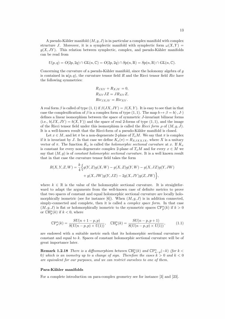
13

A pseudo-Kahler manifold (M, g, J) is in particular a complex manifold with complexstructure J . Moreover, it is a symplectic manifold with symplectic form ω(X,Y ) =g(X, JY ). This relation between symplectic, complex, and pseudo-Kahler manifoldscan be read from

U(p, q) = O(2p, 2q) ∩GL(n,C) = O(2p, 2q) ∩ Sp(n,R) = Sp(n,R) ∩GL(n,C).

Concerning the curvature of a pseudo-Kahler manifold, since the holonomy algebra of gis contained in u(p, q), the curvature tensor field R and the Ricci tensor field Ric havethe following symmetries:

RJXY +RXJY = 0,

RXY JZ = JRXY Z,

RicJXJY = RicXY .

A real form β is called of type (1, 1) if β(JX, JY ) = β(X,Y ). It is easy to see that in thatcase the complexification of β is a complex form of type (1, 1). The map b 7→ β = b(·, J ·)defines a linear isomorphism between the space of symmetric J-invariant bilinear forms(i.e., b(JX, JY ) = b(X,Y )) and the space of real 2-forms of type (1, 1), and the imageof the Ricci tensor field under this isomorphism is called the Ricci form ρ of (M, g, J).It is a well-known result that the Ricci-form of a pseudo-Kahler manifold is closed.

Let x ∈M , and let π be a non-degenerate 2-plane of TxM . We say that π is complexif it is invariant by J . In that case we define Kx(π) = RXJXXJX , where X is a unitaryvector of π. The function Kx is called the holomorphic sectional curvature at x. If Kx

is constant for every non-degenerate complex 2-plane of TxM and for every x ∈ M wesay that (M, g) is of constant holomorphic sectional curvature. It is a well known resultthat in that case the curvature tensor field takes the form

R(X,Y, Z,W ) =k

4

g(Y,Z)g(X,W )− g(X,Z)g(Y,W )− g(X, JZ)g(Y, JW )

+ g(X, JW )g(Y, JZ)− 2g(X, JY )g(Z, JW ),

where k ∈ R is the value of the holomorphic sectional curvature. It is straightfor-ward to adapt the arguments from the well-known case of definite metrics to provethat two spaces of constant and equal holomorphic sectional curvature are locally holo-morphically isometric (see for instance [6]). When (M, g, J) is in addition connected,simply-connected and complete, then it is called a complex space form. In that case(M, g, J) is flat or holomorphically isometric to the symmetric spaces CPnp (k) if k > 0or CHn

p (k) if k < 0, where

CPnp (k) =SU(n+ 1− p, p)

S(U(n− p, p)×U(1)), CHn

p (k) =SU(n− p, p+ 1)

S(U(n− p, p)×U(1)), (1.1)

are endowed with a suitable metric such that its holomorphic sectional curvature isconstant and equal to k. Spaces of constant holomorphic sectional curvature will be ofgreat importance later.

Remark 1.2.18 There is a diffeomorphism between CHnp (k) and CPnn−p(−k) (for k <

0) which is an isometry up to a change of sign. Therefore the cases k > 0 and k < 0are equivalent for our purposes, and we can restrict ourselves to one of them.

Para-Kahler manifolds

For a complete introduction on para-complex geometry see for instance [3] and [23].

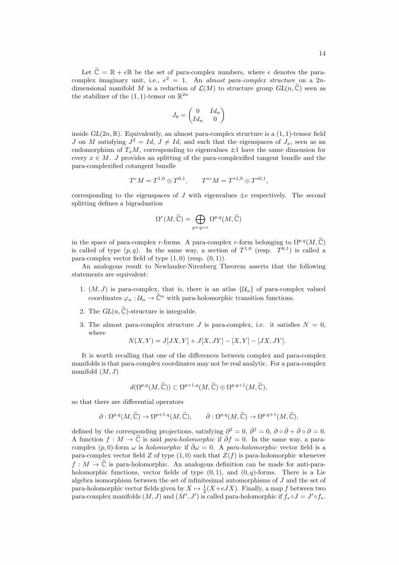
14

Let C = R + eR be the set of para-complex numbers, where e denotes the para-complex imaginary unit, i.e., e2 = 1. An almost para-complex structure on a 2n-dimensional manifold M is a reduction of L(M) to structure group GL(n, C) seen asthe stabilizer of the (1, 1)-tensor on R2n

J0 =

(0 IdnIdn 0

)inside GL(2n,R). Equivalently, an almost para-complex structure is a (1, 1)-tensor fieldJ on M satisfying J2 = Id, J 6= Id, and such that the eigenspaces of Jx, seen as anendomorphism of TxM , corresponding to eigenvalues ±1 have the same dimension forevery x ∈ M . J provides an splitting of the para-complexified tangent bundle and thepara-complexified cotangent bundle

T cM = T 1,0 ⊕ T 0,1, T ∗cM = T ∗1,0 ⊕ T ∗0,1,

corresponding to the eigenspaces of J with eigenvalues ±e respectively. The secondsplitting defines a bigraduation

Ωr(M, C) =⊕p+q=r

Ωp,q(M, C)

in the space of para-complex r-forms. A para-complex r-form belonging to Ωp,q(M, C)is called of type (p, q). In the same way, a section of T 1,0 (resp. T 0,1) is called apara-complex vector field of type (1, 0) (resp. (0, 1)).

An analogous result to Newlander-Nirenberg Theorem asserts that the followingstatements are equivalent:

1. (M,J) is para-complex, that is, there is an atlas Uα of para-complex valued

coordinates ϕα : Uα → Cn with para-holomorphic transition functions.

2. The GL(n, C)-structure is integrable.

3. The almost para-complex structure J is para-complex, i.e. it satisfies N = 0,where

N(X,Y ) = J [JX, Y ] + J [X, JY ]− [X,Y ]− [JX, JY ].

It is worth recalling that one of the differences between complex and para-complexmanifolds is that para-complex coordinates may not be real analytic. For a para-complexmanifold (M,J)

d(Ωp,q(M, C)) ⊂ Ωp+1,q(M, C)⊕ Ωp,q+1(M, C),

so that there are differential operators

∂ : Ωp,q(M, C)→ Ωp+1,q(M, C), ∂ : Ωp,q(M, C)→ Ωp,q+1(M, C),

defined by the corresponding projections, satisfying ∂2 = 0, ∂2 = 0, ∂ ∂ + ∂ ∂ = 0.A function f : M → C is said para-holomorphic if ∂f = 0. In the same way, a para-complex (p, 0)-form ω is holomorphic if ∂ω = 0. A para-holomorphic vector field is apara-complex vector field Z of type (1, 0) such that Z(f) is para-holomorphic whenever

f : M → C is para-holomorphic. An analogous definition can be made for anti-para-holomorphic functions, vector fields of type (0, 1), and (0, q)-forms. There is a Liealgebra isomorphism between the set of infinitesimal automorphisms of J and the set ofpara-holomorphic vector fields given by X 7→ 1

2 (X+eJX). Finally, a map f between twopara-complex manifolds (M,J) and (M ′, J ′) is called para-holomorphic if f∗J = J ′f∗.

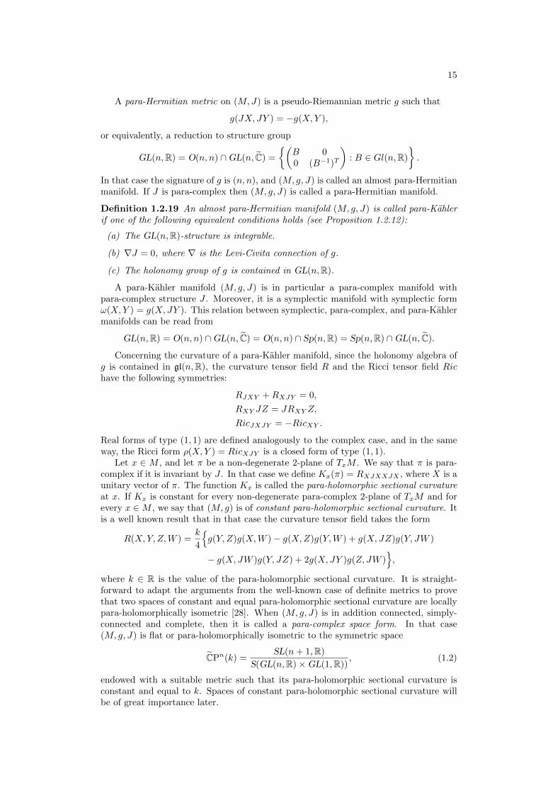
15

A para-Hermitian metric on (M,J) is a pseudo-Riemannian metric g such that

g(JX, JY ) = −g(X,Y ),

or equivalently, a reduction to structure group

GL(n,R) = O(n, n) ∩GL(n, C) =

(B 00 (B−1)T

): B ∈ Gl(n,R)

.

In that case the signature of g is (n, n), and (M, g, J) is called an almost para-Hermitianmanifold. If J is para-complex then (M, g, J) is called a para-Hermitian manifold.

Definition 1.2.19 An almost para-Hermitian manifold (M, g, J) is called para-Kahlerif one of the following equivalent conditions holds (see Proposition 1.2.12):

(a) The GL(n,R)-structure is integrable.

(b) ∇J = 0, where ∇ is the Levi-Civita connection of g.

(c) The holonomy group of g is contained in GL(n,R).

A para-Kahler manifold (M, g, J) is in particular a para-complex manifold withpara-complex structure J . Moreover, it is a symplectic manifold with symplectic formω(X,Y ) = g(X, JY ). This relation between symplectic, para-complex, and para-Kahlermanifolds can be read from

GL(n,R) = O(n, n) ∩GL(n, C) = O(n, n) ∩ Sp(n,R) = Sp(n,R) ∩GL(n, C).

Concerning the curvature of a para-Kahler manifold, since the holonomy algebra ofg is contained in gl(n,R), the curvature tensor field R and the Ricci tensor field Richave the following symmetries:

RJXY +RXJY = 0,

RXY JZ = JRXY Z,

RicJXJY = −RicXY .

Real forms of type (1, 1) are defined analogously to the complex case, and in the sameway, the Ricci form ρ(X,Y ) = RicXJY is a closed form of type (1, 1).

Let x ∈ M , and let π be a non-degenerate 2-plane of TxM . We say that π is para-complex if it is invariant by J . In that case we define Kx(π) = RXJXXJX , where X is aunitary vector of π. The function Kx is called the para-holomorphic sectional curvatureat x. If Kx is constant for every non-degenerate para-complex 2-plane of TxM and forevery x ∈M , we say that (M, g) is of constant para-holomorphic sectional curvature. Itis a well known result that in that case the curvature tensor field takes the form

R(X,Y, Z,W ) =k

4

g(Y,Z)g(X,W )− g(X,Z)g(Y,W ) + g(X, JZ)g(Y, JW )

− g(X, JW )g(Y, JZ) + 2g(X, JY )g(Z, JW ),

where k ∈ R is the value of the para-holomorphic sectional curvature. It is straight-forward to adapt the arguments from the well-known case of definite metrics to provethat two spaces of constant and equal para-holomorphic sectional curvature are locallypara-holomorphically isometric [28]. When (M, g, J) is in addition connected, simply-connected and complete, then it is called a para-complex space form. In that case(M, g, J) is flat or para-holomorphically isometric to the symmetric space

CPn(k) =SL(n+ 1,R)

S(GL(n,R)×GL(1,R)), (1.2)

endowed with a suitable metric such that its para-holomorphic sectional curvature isconstant and equal to k. Spaces of constant para-holomorphic sectional curvature willbe of great importance later.

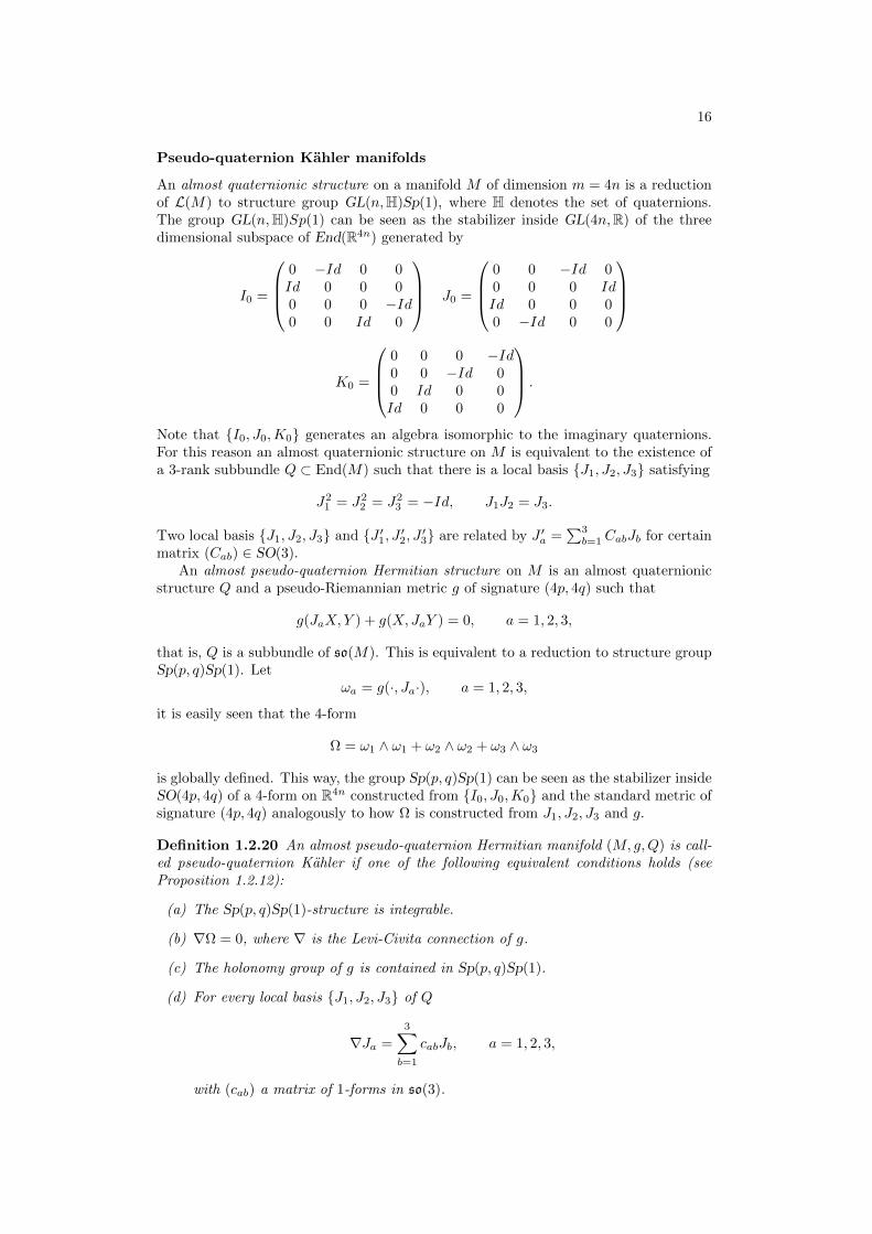
16

Pseudo-quaternion Kahler manifolds

An almost quaternionic structure on a manifold M of dimension m = 4n is a reductionof L(M) to structure group GL(n,H)Sp(1), where H denotes the set of quaternions.The group GL(n,H)Sp(1) can be seen as the stabilizer inside GL(4n,R) of the threedimensional subspace of End(R4n) generated by

I0 =

0 −Id 0 0Id 0 0 00 0 0 −Id0 0 Id 0

J0 =

0 0 −Id 00 0 0 IdId 0 0 00 −Id 0 0

K0 =

0 0 0 −Id0 0 −Id 00 Id 0 0Id 0 0 0

.

Note that I0, J0,K0 generates an algebra isomorphic to the imaginary quaternions.For this reason an almost quaternionic structure on M is equivalent to the existence ofa 3-rank subbundle Q ⊂ End(M) such that there is a local basis J1, J2, J3 satisfying

J21 = J2

2 = J23 = −Id, J1J2 = J3.

Two local basis J1, J2, J3 and J ′1, J ′2, J ′3 are related by J ′a =∑3b=1 CabJb for certain

matrix (Cab) ∈ SO(3).An almost pseudo-quaternion Hermitian structure on M is an almost quaternionic

structure Q and a pseudo-Riemannian metric g of signature (4p, 4q) such that

g(JaX,Y ) + g(X, JaY ) = 0, a = 1, 2, 3,

that is, Q is a subbundle of so(M). This is equivalent to a reduction to structure groupSp(p, q)Sp(1). Let

ωa = g(·, Ja·), a = 1, 2, 3,

it is easily seen that the 4-form

Ω = ω1 ∧ ω1 + ω2 ∧ ω2 + ω3 ∧ ω3

is globally defined. This way, the group Sp(p, q)Sp(1) can be seen as the stabilizer insideSO(4p, 4q) of a 4-form on R4n constructed from I0, J0,K0 and the standard metric ofsignature (4p, 4q) analogously to how Ω is constructed from J1, J2, J3 and g.

Definition 1.2.20 An almost pseudo-quaternion Hermitian manifold (M, g,Q) is call-ed pseudo-quaternion Kahler if one of the following equivalent conditions holds (seeProposition 1.2.12):

(a) The Sp(p, q)Sp(1)-structure is integrable.

(b) ∇Ω = 0, where ∇ is the Levi-Civita connection of g.

(c) The holonomy group of g is contained in Sp(p, q)Sp(1).

(d) For every local basis J1, J2, J3 of Q

∇Ja =

3∑b=1

cabJb, a = 1, 2, 3,

with (cab) a matrix of 1-forms in so(3).

17

The fact that (d) is equivalent to (a), (b) and (c) is actually a result by Ishihara[35, 36]. However, since so far the present author has not found a complete proof of thisresult, we exhibit a simple proof here.

Proof of Ishihara’s Theorem. Suppose that (M, g,Q) has holonomy contained inSp(p, q)Sp(1). Let P be the holonomy bundle, which is a reduction of O(M) to structuregroup Sp(p, q)Sp(1). The group Sp(1) can be seen as the group S3 ⊂ H of quaternionsof norm 1 (that is, qq = 1), so that it acts on the imaginary quaternions Im(H) as

Lq : Im(H) → Im(H)z 7→ qzq.

Under the identification Im(H) = R3, Lq is an element of SO(3) determining a 1 : 2covering Sp(1)→ SO(3). We consider the associated bundle

Q = P ×Sp(p,q)Sp(1) R3,

where Sp(p, q)Sp(1) acts on R3 through the action of Sp(1) described above. This vectorbundle is seen as a three rank subbundle of End(M) by

P ×Sp(n)Sp(1) R3 → P ×Sp(n)Sp(1) End(R4n)[v, ξ] 7→ [v, ξ1I0 + ξ2J0 + ξ3K0].

It is easy to see that a local section σ of P determines a local basis J1 = [σ, e1],J2 = [σ, e2], J3 = [σ, e3] of Q which satisfies

J21 = J2

2 = J23 = −Id, J1J2 = J3,

that is, Q is an almost quaternionic structure. Let τ be a curve in M and S0 = [u0, ξ] ∈Q. The horizontal lift of τ to S0 in End(M) is just the curve [ut, ξ], where ut is thehorizontal lift of τ to u0. By definition ut is contained in P, so that [ut, ξ] is containedin Q. This means that Q is invariant by parallel transport. Therefore, let τ t0 denote theparallel transport along τ from t = 0 to t, there is a matrix (Cab(t)) ∈ SO(3) such that

τ t0(Ja) =

3∑b=1

Cab(t)Jb, a = 1, 2, 3.

differentiating at t = 0 we find that

∇XJa =

3∑b=1

cabJb, a = 1, 2, 3,

where X = τ(t = 0), and cab = ddt

∣∣t=0

Cab(t) ∈ so(3). Conversely, suppose that

∇XJa =

3∑b=1

cabJb, a = 1, 2, 3.

Since ∇g = 0 we have that

∇Xωa =

3∑b=1

cabωb, a = 1, 2, 3,

and thus a straightforward computation shows that ∇Ω = 0.

18

Regarding the curvature, we will say that an algebraic curvature tensor R is of typesp(p, q) if it sits in 2sp(p, q) when seen as an element of 2so(4p, 4q). This kind oftensors satisfies the following symmetries:

RJaXY +RXJaY = 0, a = 1, 2, 3,

RXY JaZ = JaRXY Z, a = 1, 2, 3,

Ric = 0.

The proof of the following proposition can be found in [2].

Proposition 1.2.21 The curvature of a pseudo-quaternion Kahler manifold (M, g,Q)decomposes as

R = νqR0 +Rsp(p,q),

where νq = s16n(n+2) , R0 is four times the curvature of the pseudo-quaternionic hyper-

bolic space (of the corresponding signature)

R0XY ZW = g(X,Z)g(Y,W )− g(Y, Z)g(X,W ) +

∑a

g(JaX,Z)g(JaY,W )

−g(JaY,Z)g(JaX,W ) + 2g(X, JaY )g(Z, JaW ) , (1.3)

and Rsp(p,q) is of type sp(p, q). In particular (M, g,Q) is Einstein.

Let x ∈ M , and let Z ∈ TxM with g(Z,Z) 6= 0. We consider the 4-dimensionalsubspace V (Z) = SpanZ, J1Z, J2Z, J3Z ⊂ TxM . Let π ⊂ V (Z) be a non-degenerate2-plane and X,Y an orthonormal basis of π, if Kx(Z)(π) = RXYXY is constant forevery π, we call Kx(Z) the quaternionic sectional curvature with respect to Z at x. Wesay that (M, g,Q) has constant quaternionic sectional curvature if Kx(Z) is constantfor every Z ∈ TxM and every x ∈ M . It is a well known result that in that case thecurvature tensor field takes the form

R =k

4R0,

where R0 is given by (1.3) and k is the value of the quaternionic sectional curvature. Itis straightforward to adapt the arguments from the well-known case of definite metricsto prove that two spaces of constant and equal quaternionic sectional curvature arelocally isometric preserving their pseudo-quaternion Kahler structures (see for instance[52]). When (M, g,Q) is in addition connected, simply-connected and complete, then itis called a quaternion space form. In that case (M, g,Q) is flat or isometric (preservingthe pseudo-quaternion Kahler structures) to the symmetric spaces HPnp (k) if k > 0 orHHn

p (k) if k < 0, where

HPnp (k) =Sp(p, n+ 1− p)Sp(p, n− p)Sp(1)

, HHnp (k) =

Sp(p+ 1, n− p)Sp(p, n− p)Sp(1)

, (1.4)

endowed with a suitable metric such that its quaternionic sectional curvature is constantand equal to k. Spaces of constant quaternionic sectional curvature will be of greatimportance later.

Remark 1.2.22 There is a diffeomorphism between HHps(k) and HPnn−p(−k) (for k <

0) which is an isometry up to a change of sign. Therefore the cases k > 0 and k < 0are equivalent for our purposes, and we can restrict ourselves to one of them.

Although pseudo-hyper-Kahler manifolds will not give many interesting results inthis thesis, this kind of manifolds are intimate related to pseudo-quaternion Kahlermanifolds and will be briefly treated later. For this reason we recall its definition. An

19

almost pseudo-hyper-complex structure on M , dimM = 4n, is a three rank subbundleof End(M) which admits a global basis J1, J2, J3 satisfying

J21 = J2

2 = J23 = −Id, J1J2 = J3,

or equivalently a reduction of L(M) to group GL(n,H), which is seen as the commonstabilizer of I0, J0,K0 inside GL(4n,R). An almost pseudo-hyper-Hermitian structureon M is an almost pseudo-hyper-complex structure J1,J2, J3 and a pseudo-Riemannianmetric of signature (4p, 4q) such that

g(JaX,Y ) + g(X, JaY ) = 0, a = 1, 2, 3,

or equivalently a reduction to structure group Sp(p, q). We thus have

Definition 1.2.23 An almost pseudo-hyper-Hermitian manifold is called pseudo-hyper-Kahler if one of the following equivalent conditions holds (see Proposition 1.2.12):

(a) The Sp(p, q)-structure is integrable.

(b) ∇Ja = 0 for a = 1, 2, 3, where ∇ is the Levi-Civita connection of g.

(c) The holonomy group of g is contained in Sp(p, q).

It is evident that the curvature tensor field of a pseudo-hyper-Kahler manifold is oftype sp(p, q).

Para-quaternion Kahler manifolds

Let H denote the set of para-quaternions (also known as split-quaternions). An almostpara-quaternionic structure on a manifold M of dimension m = 4n is a reduction ofL(M) to structure group GL(n, H)Sp(1,R). The group GL(n, H)Sp(1,R) can be seen asthe stabilizer inside GL(4n,R) of the three dimensional subspace of End(R4n) generatedby

I0 =

0 −Id 0 0Id 0 0 00 0 0 −Id0 0 Id 0

J0 =

0 Id 0 0Id 0 0 00 0 0 Id0 0 Id 0

K0 =

−Id 0 0 0

0 Id 0 00 0 −Id 00 0 0 Id

.

Note that I0, J0,K0 generates an algebra isomorphic to the set of imaginary para-quaternions. For this reason an almost para-quaternionic structure on M is equivalentto the existence of a three rank subbundle Q ⊂ End(M) such that there is a local basisJ1, J2, J3 satisfying

J21 = −Id, J2

2 = J23 = Id, J1J2 = J3.

Two local basis J1, J2, J3 and J ′1, J ′2, J ′3 are related by J ′a =∑3b=1 CabJb for certain

matrix (Cab) ∈ SO(1, 2).A pseudo-Riemannian manifold of signature (r, s) is said strongly oriented if the

bundle of orthonormal frames can be reduced to the connected component SO0(r, s)(since SO(r, s)/SO0(r, s) is discrete there always exists a strongly oriented cover of M).

An almost para-quaternion Hermitian structure on a strongly oriented pseudo-Rie-mannian manifold (M, g) of signature (2n, 2n) is an almost para-quaternionic structureQ such that

g(JaX,Y ) + g(X, JaY ) = 0, a = 1, 2, 3,

20

that is, Q is a subbundle of so(M). This is equivalent to a reduction to structure groupSp(n,R)Sp(1,R) ⊂ SO0(2n, 2n). Let

ωa = g(·, Ja·), a = 1, 2, 3,

it is easily seen that the 4-form

Ω = ω1 ∧ ω1 − ω2 ∧ ω2 − ω3 ∧ ω3

is globally defined. This way, the group Sp(n,R)Sp(1,R) can be seen as the stabilizerinside SO0(2n, 2n) of a 4-form on R4n constructed from I0, J0,K0 and the standardmetric of signature (2n, 2n) analogously to how Ω is constructed from J1, J2, J3 and g.

Definition 1.2.24 An almost para-quaternion Hermitian manifold (M, g,Q) is calledpara-quaternion Kahler if one of the following equivalent conditions holds (see Proposi-tion 1.2.12):

(a) The Sp(n,R)Sp(1,R)-structure is integrable.

(b) ∇Ω = 0, where ∇ is the Levi-Civita connection of g.

(c) The holonomy of g is contained in Sp(n,R)Sp(1,R).

(d) For every local basis J1, J2, J3 of Q

∇Ja =

3∑b=1

cabJb, a = 1, 2, 3,

with (cab) a matrix of 1-forms in so(1, 2).

The fact that (d) is equivalent to (a), (b) and (c) can be proved analogously to thepseudo-quaternion Kahler case.

Regarding the curvature, we will say that an algebraic curvature tensor R is of typesp(n,R) if it sits in 2sp(n,R) when seen as an element of 2so(2n, 2n). This kind oftensors satisfy the following symmetries:

RJaXY +RXJaY = 0, a = 1, 2, 3,

RXY JaZ = JaRXY Z, a = 1, 2, 3,

Ric = 0.

The proof of the following proposition can be found in [2].

Proposition 1.2.25 A para-quaternion Kahler manifold (M, g,Q) has curvature tensorfield

R = νqR0 +Rsp(n,R),

where νq = s16n(n+2) , R0 is four times the curvature of the para-quaternionic hyperbolic

space (of the corresponding signature)

R0XY ZW = g(X,Z)g(Y,W )− g(Y, Z)g(X,W )−

∑a

εa g(JaX,Z)g(JaY,W )

−g(JaY,Z)g(JaX,W ) + 2g(X, JaY )g(Z, JaW ) , (1.5)

with (ε1, ε2, ε3) = (−1, 1, 1) and Rsp(n,R) is of type sp(n,R). In particular (M, g,Q) isEinstein.

21

Let x ∈ M , and let Z ∈ TxM with g(Z,Z) 6= 0. We consider the 4-dimensionalsubspace V (Z) = SpanZ, J1Z, J2Z, J3Z ⊂ TxM . Let π ⊂ V (Z) be a non-degenerate2-plane and X,Y an orthonormal basis of π, if Kx(Z)(π) = RXYXY is constant forevery π, we call Kx(Z) the para-quaternionic sectional curvature with respect to Z atx. We say that (M, g,Q) has constant para-quaternionic sectional curvature if Kx(Z)is constant for every Z ∈ TxM and every x ∈M . It is a well known result that in thatcase the curvature tensor field takes the form

R =k

4R0,

where R0 is given by (1.5) and k is the value of the para-quaternionic sectional curvature.It is straightforward to adapt the arguments from the well-known case of definite metricsto prove that two spaces of constant and equal para-quaternionic sectional curvatureare locally isometric preserving their para-quaternion Kahler structures (see for instance[62]). When (M, g,Q) is in addition connected, simply-connected and complete, thenit is called a para-quaternion space form. In that case (M, g,Q) is flat or isometric(preserving the para-quaternion Kahler structures) to the symmetric space

HPn(k) =Sp(n+ 1,R)

Sp(n,R)Sp(1,R)(1.6)

endowed with a suitable metric such that its para-quaternionic sectional curvature isconstant and equal to k. Spaces of constant para-quaternionic sectional curvature willbe of great importance later.

Although again para-hyper-Kahler manifolds will not give many interesting resultsin this thesis, this kind of manifolds are intimate related to para-quaternion Kahlermanifolds and will be briefly treated later. For this reason we recall its definition. Analmost para-hyper-complex structure on M , dimM = 4n, is a three rank subbundle ofEnd(M) which admits a global basis J1, J2, J3 satisfying

J21 = −Id, J2

2 = J23 = Id, J1J2 = J3,

or equivalently a reduction of L(M) to group GL(n, H), which is seen as the commonstabilizer inside GL(4n,R) of I0, J0,K0. An almost para-hyper-Hermitian structure onM is an almost para-hyper-complex structure J1, J2, J3 and a pseudo-Riemannianmetric of signature (2n, 2n) such that

g(JaX,Y ) + g(X, JaY ) = 0, a = 1, 2, 3,

or equivalently a reduction to structure group Sp(n,R). We thus have

Definition 1.2.26 An almost para-hyper-Hermitian manifold (M, g, J1, J2, J3) is calledpara-hyper-Kahler if one of the following equivalent conditions holds (see Proposition1.2.12):

(a) The Sp(n,R)-structure is integrable.

(b) ∇Ja = 0 for a = 1, 2, 3, where ∇ is the Levi-Civita connection of g.

(c) The holonomy group of g is contained in Sp(n,R).

It is evident that the curvature tensor field of a para-hyper-Kahler manifold is oftype sp(n,R).

22

Sasakian and cosymplectic manifolds

For a complete introduction to Sasakian and cosymplectic structures, and for detailedproofs see [12, 58].

Definition 1.2.27 1. An almost contact structure on a 2n+1-dimensional manifoldM is a triple (φ, ξ, η), where φ is a tensor field of type (1, 1), ξ is a vector fieldand η is a 1-form, such that

η(ξ) = 1, η φ = 0, φ2 = −id + η ⊗ ξ.

2. Let g be a pseudo-Riemannian metric on M , (φ, ξ, η, g) is called an almost contactmetric structure if (φ, ξ, η, g) is an almost contact structure and

g(ξ, ξ) = ε ∈ ±1, η = εξ[, g(φX, φY ) = g(X,Y )− εη(X)η(Y ),

for any vector fields X,Y .

An almost contact metric structure on M is equivalent to a reduction to structuregroup U(p, q)×1. Here, U(p, q)×1 is the subgroup of O(2p+1, 2q) or O(2p, 2q+1)(depending on the value of ε) stabilizing ξ0 = e2n+1 and

φ0 =

(J0 00 1

),

where e1, . . . , e2n+1 is the canonical basis of R2n+1 = R2n⊕R, and J0 is the standardcomplex structure on R2n. Here R2n+1 is assumed to be endowed with the scalar product〈 , 〉 = 〈 , 〉R2n +εe2n+1⊗e2n+1, where 〈 , 〉R2n is the standard scalar product of signature(p, q) on R2n. We define the fundamental 2-form associated to the almost contact metricstructure (φ, ξ, η, g) as Φ = g(·, φ·). In addition, in analogy with the Nijenhuis tensorfield for complex manifolds we define (see [12])

[φ, φ](X,Y ) = φ2[X,Y ] + [φX, φY ]− φ[φX, Y ]− φ[X,φY ].

Definition 1.2.28 An almost contact metric structure (φ, ξ, η, g) is called cosymplecticif one of the following equivalent conditions hold:

(a) The U(p, q)× 1-structure is integrable.

(b) (φ, ξ, η, g) satisfies [φ, φ] = 0, dη = 0, and dΦ = 0.

(c) ∇φ = 0 (which implies ∇η = 0 and ∇ξ = 0).

(d) The holonomy group of g is contained in U(p, q)× 1.

Definition 1.2.29 An almost contact metric structure (φ, ξ, η, g) is said to be Sasakianif one of the following equivalent conditions hold:

1. (φ, ξ, η, g) satisfies [φ, φ] + 2η ⊗ ξ = 0, and dη = Φ.

2. (∇Xφ)Y = g(X,Y )ξ − εη(Y )X.

Note that Sasakian geometry is not an integrable geometry, in the sense that theholonomy group is not contained in U(p, q)×1, that is, the U(p, q)×1-structured de-termined by the almost contact metric structure is not integrable. This fact will requirea slight modification when classifying homogeneous Sasakian structures in Chapter 4.In order to do that a few words about the intrinsic torsion of an almost contact metricstructure must be said (for an excellent introduction to the intrinsic torsion of a G-structure see [53, 26]). As we have seen above, the U(p, q) × 1-structure determined

23

by the almost contact metric structure (φ, ξ, η, g) is integrable if and only if ∇φ = 0 (orequivalently if and only if ∇Φ = 0). We can thus see the tensor field ∇φ (or ∇Φ) asthe obstruction for (φ, ξ, η, g) to be cosymplectic. Therefore, one can study the possiblenon-integrable geometries an almost contact metric manifold can present by studyingthe possible tensor fields ∇φ (or ∇Φ) arising. This can be done considering the vectorspace V = R2n+1 endowed with the standard almost contact metric structure describedabove. We then take the space C(V ) of tensors of type (0, 3) with the same symmetriesas ∇Φ, that is,

TXY Z = −TXY Z = −TXφY φZ + η(Y )TXξZ + η(Z)TXY ξ.

C(V ) is an U(p, q) × 1-module in a natural way, so that one can decompose it intoirreducible V -submodules. This was achieve in [22] for the Riemannian case obtainingtwelve irreducible submodules, and the case of metrics with signature is obtained by astraightforward adaptation. Each of this submodules determines a class of geometricstructures. The class corresponding to the so called α-Sasakian structures is given bythe submodule

C6(V ) = T ∈ C(V )/TXY Z = αε (〈X,Y 〉η(Z)− 〈X,Z〉η(Y )) , α ∈ R ,

from which Sasakian structures corresponds to α = 1. This will be used in section 4.2.6.We finally recall the notion of φ-sectional curvature. Let

Dx = X ∈ TxM, η(X) = 0.

If X ∈ TxM is a unitary vector, then X and φX span a non-degenerate plane π, andhence we can consider the sectional curvature Kx(π) = RXφXXφX of that plane. If Kx

is constant for all unitary vectors X ∈ Dx and every x ∈ M , then we say that M is ofconstant φ-sectional curvature. In that case the curvature tensor field takes the form

4R(X,Y )Z = (k + 3ε)g(Y,Z)X − g(X,Z)Y + (εk − 1)η(X)η(Z)Y − η(Y )η(Z)X+ (k − ε) g(X,Z)η(Y )ξ − g(Y, Z)η(X)ξ

+ g(φY,Z)φX + g(φZ,X)φY − 2g(φX, Y )φZ ,

where k is the constant value of the φ-sectional curvature.

1.3 Homogeneous spaces and the canonicalconnection

Let G be a Lie group and H a subgroup. It is a classic problem to try to endow thequotient G/H with a “good” differentiable structure, that is a differentiable structuresuch that π : G → G/H is a submersion. This is not always possible, and the mainproblem is to ensure that the quotient topology is Hausdorff. It is easy to see that thequotient G/H is Hausdorff if and only if H is a closed subgroup of G. In fact we havethe following well known result (see [38, Ch. I]).

Theorem 1.3.1 Let G be a Lie group and H a closed subgroup of G. Then there is aunique differentiable structure on G/H such that the action of G on G/H is C∞, thatis, the mapping G×G/H → G/H, (a, bH) 7→ abH is C∞. In particular π : G→ G/His a submersion. In addition, dimG/H = dimG− dimH.

Note that for every two points aH, bH ∈ G/H the differentiable mapping induced bythe left translation by ab−1 takes the point bH to aH, implying that the orbit of a pointaH by the action of G is the whole G/H. This fact suggests the following equivalentdefinitions.

24

Definition 1.3.2 (Definition of homogeneous space 1) A homogeneous space is aquotient G/H of a Lie group G by a closed subgroup H, endowed with the unique dif-ferentiable structure making π : G→ G/H a submersion.

Definition 1.3.3 (Definition of homogeneous space 2) A manifold M is homoge-neous if there is a Lie group G acting on the left on M , such that the action is C∞ andtransitive.

We shall denote by La : M →M the action of an element a ∈ G. We shall also oftendenote by a · p the action of a ∈ G on a point p. The equivalence between the previoustwo definitions is given by the following construction. Let G/H be the quotient of a Liegroup G by a closed subgroup H, then G acts on G/H by left translations, and as wehave seen this action is transitive. Conversely, let M be a manifold on which G actstransitively. We define the isotropy group at a point p ∈M as the subgroup

H = a ∈ G/a · p = p.

H is a closed subgroup of G and it is a straightforward computation to see that the map

G/H → MaH 7→ a · p

defines a diffeomorphism between G/H and M . Note that in both cases G→ G/H is aprincipal bundle with structure group H. A group G is said to act effectively on M ifthe subgroup

N = a ∈ G/La = IdM

only contains the neutral element of G. Since N is a normal subgroup of G, we canalways assume that G acts effectively on M replacing G by G/N .

Definition 1.3.4 A pseudo-Riemannian manifold (M, g) is called homogeneous if thereis a Lie group G of isometries acting transitively on the left on M .

If a connected pseudo-Riemannian manifold is homogeneous then the isometry groupIsom(M) and Isom0(M, g) acts transitively on M , where Isom0(M, g) is the connectedcomponent of Isom(M, g) containing the identity. Moreover, G can be identify with aLie subgroup of Isom(M, g).

Remark 1.3.5 It can be proved (see [38, Ch. I]) that a homogeneous manifold alwaysadmits a real analytic structure, such that the action G×G/H → G/H and the projectionG→ G/H are real analytic maps. Although most of the time we will only be concernedabout C∞ structures and maps, we will make use of this fact when necessary.

As we have seen, homogeneous spaces enjoy a large group of internal symmetries.For that reason they constitute a distinguished class of spaces on which the study ofpseudo-Riemannian geometry is especially rich and varied. However, this privilegedposition is often paid with their rigidity. Weakening Definition 1.3.3 we can obtain alarger and less rigid class of spaces which still share most of the desirable properties ofhomogeneous spaces.

Definition 1.3.6 A pseudo-Riemannian manifold (M, g) is called locally homogeneousif the pseudo-group of local isometries acts transitively on (M, g), that is, if for everytwo points p, q ∈ M there are neighborhoods U and V of p and q respectively, and anisometry f : U → V taking p to q.

The following definition will be central for the rest of this dissertation.

25

Definition 1.3.7 A homogeneous space G/H is called reductive if the Lie algebra gof G can be decomposed as g = h ⊕ m, where h is the Lie algebra of H and m is anAd(H)-invariant subspace, that is, Adh(m) ⊂ m for every h ∈ H.

The condition Ad(H)(m) ⊂ m implies [h,m] ⊂ m, and the converse holds if H isconnected. Note that we can identify the subspace m with ToM , where o = H ∈ G/His the origin of G/H, as follows: let X ∈ m, we consider the one parameter groupexp(tX), and identify X with X∗o , where X∗ is the fundamental vector field associatedto X defined by

X∗p =d

dt

∣∣∣∣t=0

Lexp(tX)(p), p ∈ G/H.

By definition it is easy to see that

[X∗, Y ∗] = −[X,Y ]∗, (Adg(X))∗Lg(p) = (Lg)∗p(X

∗p ).

Proposition 1.3.8 Every homogeneous Riemannian space (M, g) is reductive.

Proof. We fix the origin o ∈M . Let M = G/H, and let g and h denote the Lie algebrasof G and H respectively. We can suppose that G acts effectively. For every X ∈ g weconsider the associated vector field X∗. It is clear that h consists of those X ∈ g suchthat X∗o = 0. Let∇ be the Levi-Civita connection of g. Since X∗ is a Killing vector field,the operator AX∗ = LX∗ −∇X = −∇X is skew-symmetric, so that AX∗|o ∈ so(ToM).Let B denote the Killing form of so(ToM), we consider the symmetric bilinear form φon g defined as

φ(X,Y ) = −B(AX∗|o, AY ∗|o).

Since g is positive definite, B is negative definite so that φ(X,X) = 0 implies thatAX∗|o = 0. Therefore, if X ∈ h and φ(X,X) = 0 we have AX∗|o and X∗o = 0, whenceX∗ = 0. Since G acts effectively we obtain X = 0. This proves that φ is definite on h.In addition, let h ∈ H, for every X,Y ∈ g

φ(Adh(X),Adh(Y )) = −B(AAdh(X)∗|o, AAdh(Y )∗|o

)= −B

(ALh∗(X∗o ), ALh∗(Y ∗o )

)= −

∑k

g (∇ekLh∗(X∗o ),∇ekLh∗(Y ∗o ))

= −∑k

g (∇ekX∗o ,∇ekY ∗o )

= φ(X,Y ),

since Lh∗ is an isometry, where ek is any orthonormal basis of ToM . This shows thatφ is Ad(H)-invariant. Finally, we take the orthogonal complement m = h⊥ of h withrespect to φ. By construction g = h⊕m and m is Ad(H)-invariant.

We now turn to define a very special invariant connection: the so called canonicalconnection. But before we need some technical preliminaries.

Lemma 1.3.9 For every X ∈ X(M) there is a unique vector field X on L(M) suchthat

1. X is invariant by the right action of GL(m,R).

2. LXθ = 0.

3. π∗(Xu) = Xπ(u) for every u ∈ L(M).

26

Moreover, for every X on L(M) satisfying (a) and (b), there is a unique vector field X

on M satisfying (c). The vector field X is called the natural lift of X.

Proof. Let ft be the one parameter group of local transformations of X, we considerthe set of induced local maps ft on L(M). The vector field X is defined as the vector

field generating ft. It is straightforward to prove uniqueness and properties (a), (b) and(c).

Let M = K/H be a homogeneous space. We denote by o ∈ M the coset H, whichwill be called the origin of M . We consider the map

H → Aut(ToM)h 7→ (Lh)∗,o.

It is immediate to see that this map is a group homomorphism, which will be calledthe linear isotropy representation. By definition, the isotropy representation is faithfulif and only if the action of K is effective, or equivalently if the induced action of K onL(M) is free. Hereafter we suppose that K is connected and the isotropy representationis faithful. We will also assume that there is a G-structure P (M,G) which is invariantby the induced action of K on L(M), that is, for every a ∈ K we have an induced map

La : P → P . Note that all the subsequent results can be applied to pseudo-Riemannianhomogeneous spaces by taking the bundle of orthonormal references O(M) as P (M,G).Let u0 ∈ P such that π(u0) = o. We say that a linear connection on P (M,G) is

invariant by the action of K if it is invariant by La for every a ∈ K.Identifying ToM with Rm through the isomorphism u0 : Rm → ToM , we can see the

linear isotropy representation as the homomorphism

λ : H → Gh 7→ λ(h) = u−1

0 (Lh)∗,o u0.(1.7)

We shall also denote by λ the corresponding homomorphism of Lie algebras λ : h→ g.Let X ∈ k, consider the one parameter subgroup exp(tX) of K, which determines a oneparameter group of transformations ft = Lexp(tX) of M . We will also denote by X the

vector field associated to ft, that is Xp = ddt

∣∣t=0

ft(p), p ∈ K/H.

Theorem 1.3.10 (Wang) Let P (M,G) be an invariant G-structure on a reductivehomogeneous space K/H with reductive decomposition k = h⊕m. Then, there is a oneto one correspondence between invariant connections on P and linear maps Λm : m→ gsuch that

Λm(Adh(X)) = Adλ(h)(Λm(X)), X ∈ m, h ∈ H.

The correspondence can be read from

ωu0(X) =

Λm(X) X ∈ mλ(X) X ∈ h

,

where ω is the 1-form of the invariant connection.

Proof. The correspondence (see [38]) is given by

Λ(X) =

λ(X) if X ∈ hΛm(X) if X ∈ m

It is obvious that the linear map Λm = 0 satisfies the condition in Theorem 1.3.10.The corresponding invariant connection thus enjoys a distinguished position amonginvariant connections and will be of great importance in this thesis.

27

Definition 1.3.11 The invariant connection corresponding to the linear map Λm = 0is called the canonical connection associated to the reductive decomposition k = h⊕m.

The canonical connection associated a certain reductive decomposition has a geo-metric characterization which is often very useful (see [38, Ch. X, Corollary 2.5]).

Proposition 1.3.12 Let P (M,G) be a K-invariant G-structure on a homogeneousspace K/H. The canonical connection associated to a reductive decomposition k = h⊕mis the unique K-invariant connection on K with the following property: let ft = exp(tX)

be the one parameter subgroup of K generated by X ∈ m, and let ft be the induced trans-formations of P , then the orbit ft(u0) is horizontal, where u0 ∈ π−1(o).

Corollary 1.3.13 Let X ∈ m, consider the curve γt = Lexp(tX)(o) in K/H. Theparallel transport along γt from o to γs coincides with the differential of fs = Lexp(sX).

Proposition 1.3.14 [38] The torsion and the curvature of the canonical connectionassociated to a reductive decomposition k = h⊕m are given by:

T (X,Y )o = [X,Y ]m, X, Y ∈ m,

(R(X,Y )Z)o = [[X,Y ]h, Z], X, Y, Z ∈ m,

where the subindex h and m indicates projection on the corresponding subspace withrespect to the reductive decomposition. In addition, let ∇ denote the covariant derivativewith respect to the canonical connection, then

∇R = 0, ∇T = 0.

Proposition 1.3.15 If a tensor field on M is invariant by the action of K, then it isparallel with respect to the canonical connection.

Proof. Let J be a K-invariant tensor field of type (k, l) on M . Let X ∈ ToM , underthe identification of ToM and m we consider ft = Lexp(tX) and the curve γt = ft(o). By

Proposition 1.3.12 the horizontal lift of γt to u0 ∈ π−1(o) is γt = ft(u0). Let

E = P ×G(⊗k(Rm)∗

)⊗(⊗lRm

)be the associated bundle of tensor fields of type (k, l), and Jo = [u0, J0]. The horizontal

lift of γt to [u0, J0] in E is given by [ft(u0), J0]. But since J is K-invariant one has

[ft(u0), J0] = Jγt . We obtain by the definition of the covariant derivative on E that

(∇J)o = 0. Since the action of K is transitive and ∇ is invariant we deduce that

∇J = 0.

The converse of the previous Proposition also holds and is part of Kiricenko’s The-orem, which will be treated in Chapter 2.

Chapter 2

Ambrose-Singer connectionsand homogeneous spaces

2.1 Symmetric spaces and Cartan’s Theorem

In this section we recall the definition and some properties of symmetric and locallysymmetric spaces. We also present Cartan’s Theorem which characterizes these spacesin terms of the covariant derivative of the curvature. This is the starting point and themotivation for Ambrose-Singer’s Theorem, which generalizes Cartan’s characterizationto homogeneous spaces. For an extensive study of symmetric and locally symmetricspaces see [34].

Let (M, g) be a connected pseudo-Riemannian space, and ∇ its Levi-Civita con-nection. For every x ∈ M we consider the symmetry sx which inverts geodesics of ∇through x. sx is a diffeomorphism from a neighborhood U of x onto itself such thatsx sx is the identity transformation, that is sx is involutive, and has x as an isolatedfixed point.

Definition 2.1.1 (M, g) is called locally symmetric if sx is a local isometry for everyx ∈M . If moreover sx extends to a global isometry of M then (M, g) is called (globally)symmetric.

It is a well-known result (see [38, Ch. XI]) that, by composing symmetries sx alongbroken geodesics, the isometry group of a symmetric space (M, g) acts transitively onM , so that a symmetric space is a homogeneous space. More precisely, let G denote theidentity component of the group of isometries, then G acts transitively on M , and wecan write M = G/H, where H is the isotropy group at a point o ∈M . Let so : M →Mbe the symmetry at o ∈ M , we consider the map σ : G → G, g 7→ so g so, whichis obviously an involutive automorphism of G. Let Gσ denote the fixed point set of σand Gσ0 its identity component, then Gσ0 ⊂ H ⊂ Gσ. The differential σ∗ : g → g isalso an involutive automorphism of Lie algebras, so that it has eigenvalues ±1. A Liealgebra with such an involutive automorphism is called a symmetric Lie algebra. It isnot hard to see that h is the eigenspace associated to +1. Denoting by m the eigenspaceassociated to −1, we have that g = h⊕m and

[h, h] ⊂ h, [h,m] ⊂ m, [m,m] ⊂ h.

In particular G/H is reductive. Identifying ToM ' m, the pseudo-Riemannian metric ginduces a non-degenerate symmetric bilinear form B on m, which is necessarily Ad(H)-invariant. Conversely, let G be a Lie group with an involutive automorphism σ, andlet H be a closed subgroup sitting between Gσ0 and Gσ. Let B be an Ad(H)-invariantnon-degenerate symmetric bilinear form on m (which is the −1-eigenspace of σ∗), thenG/H can be endowed with a G-invariant pseudo-Riemannian metric g making (G/H, g)a symmetric space. In fact, under the identification m ' To(G/H), g is the G-invariantmetric on G/H with go = B. In addition, let π : G → G/H denote the canonical

29

30

projection, the map so π = π σ determines an isometric involution with fixed pointo, which can be transported by the action of G obtaining isometric involutions at everypoint of G/H.

Theorem 2.1.2 (E. Cartan) A pseudo-Riemannian manifold (M, g) is locally sym-metric if and only if ∇R = 0, where ∇ is the Levi-Civita connection of g and R itscurvature tensor field. If M is simply-connected and complete then (M, g) is symmetricif and only if ∇R = 0.

Although we don’t include the proof of this theorem (see for instance [38, Ch. XI]),it is very interesting to point out some of the arguments used, specially when comparingwith the arguments used in the proof of Ambrose-Singer’s Theorem presented in thenext section. Starting from a symmetric space (G/H, σ, g), we consider the canonicalconnection associated to the reductive decomposition g = h ⊕ m, where h and m arethe eigenspaces of σ corresponding to ±1 as before. One proves that this connectionhas vanishing torsion, and since g is G-invariant it is also metric, so that it coincideswith the Levi-Civita connection of g. This implies that ∇R = 0 by the properties ofthe canonical connection. On the other hand, let (M, g) be such that ∇R = 0. Fixinga point x ∈M one considers

g = hol⊕ TxM,

where hol is the Lie algebra of the holonomy group Hol of g. Note that since ∇R = 0, Ris invariant by the action of Hol, and so is by the action of hol. Therefore, the brackets

[A,B] = AB −BA, A,B ∈ hol,

[A,X] = A ·X, A ∈ hol, X ∈ TxM,

[X,Y ] = RXY , X, Y ∈ TxM,

endow g with a Lie algebra structure such that σ∗ : g → g with σ|TxM = −id andσ|hol = id is an involutive automorphism, that is (g, σ∗) is a symmetric Lie algebra.Consider the simply-connected Lie group G with Lie algebra g, and its connected Liesubgroup H with Lie group hol. σ∗ induces an involutive automorphism σ : G → Gsuch that H is the connected component of Gσ, hence H is closed in G and we cantake the homogeneous space G/H. Finally, the G-invariant pseudo-Riemannian metricg inherited from g at TxM makes (G/H, σ, g) a symmetric space, which is moreoverlocally isometric to (M, g).

2.2 Ambrose-Singer and Kiricenko’s Theorems

As we have seen, Cartan’s Theorem characterizes (locally) symmetric spaces as pseudo-Riemannian manifolds whose curvature tensor is covariantly constant. Moreover, whenthe manifold is globally symmetric, this approach allows us to recover a coset repre-sentation of the manifold. In this section we present Ambrose-Singer’s Theorem, whichgeneralizes Cartan’s Theorem to the more general framework of homogeneous spaces.Under suitable topological conditions, this result characterizes homogeneous spaces bythe existence of a metric connection ∇ with respect to which the curvature tensor fieldof the metric and the torsion of ∇ have vanishing covariant derivative. Furthermore, itprovides a method to recover a coset representation of the manifold, which, at least ata Lie algebra level, is achieved in terms of an elementary construction. This topic willbe studied in the next section. Ambrose-Singer’s Theorem is completed by Kiricenko’sTheorem, which extends the theory to manifolds with a geometric structure given by aset of tensor fields.

Theorem 2.2.1 (Ambrose-Singer) Let (M, g) be a connected, simply-connected andcomplete pseudo-Riemannian manifold. The following are equivalent:

31

(a) (M, g) is a reductive homogeneous pseudo-Riemannian manifold.

(b) (M, g) admits a linear connection ∇ satisfying

∇g = 0, ∇R = 0, ∇S = 0, (2.1)

where S = ∇−∇, ∇ is the Levi-Civita connection of g, and R its curvature tensorfield.

This theorem was proved by Ambrose and Singer in [4] for Riemannian metrics, andlater in [31] it was generalized to metrics of arbitrary signature.

Proposition 2.2.2 Equations (2.1) are equivalent to

∇g = 0, ∇R = 0, ∇T = 0,

where R and T are the curvature and torsion tensor fields of ∇ respectively.

Proof. The equivalence follows by direct calculation from the relations

TXY = SYX − SXY,

RXY = RXY + [SX , SY ] + STXY .

Before enouncing and proving Kiricenko’s Theorem we will need the following tech-nical Lemma (see [60] and the proof therein).

Lemma 2.2.3 Let M be a connected and simply-connected manifold of dimension m.Let X1, . . . , Xm be vector fields such that

(a) X1, . . . , Xm are complete.

(b) X1, . . . , Xm are linearly independent at every point p ∈M .

(c) [Xi, Xj ] =∑mk=1 c

kijXk, with ckij constant.

Then, fixing a point p ∈ M , M has a unique structure of Lie group such that p is theneutral element and X1, . . . , Xm is a basis of left-invariant vector fields.

Theorem 2.2.4 (Kiricenko) Let (M, g) be a connected, simply-connected and com-plete pseudo-Riemannian manifold with a geometric structure defined by a set of tensorfields P1, . . . , Pn. The following are equivalent:

(a) (M, g) is reductive homogeneous such that P1, . . . , Pn are invariant.

(b) (M, g) admits a linear connection ∇ satisfying

∇g = 0, ∇R = 0, ∇S = 0, ∇Pi = 0, (2.2)

for i = 1, . . . , n, where S = ∇ − ∇, ∇ is the Levi-Civita connection of g, and Rits curvature tensor field.

Kiricenko’s Theorem appears for the first time in [37], although Sekigawa in [54]had obtained the same result for almost Hermitian manifolds. Nevertheless, the proofappearing in the original paper by Kiricenko is incomplete, and despite the fact thatthis result has been extensively used since then, there is not a complete proof of it in theliterature as far as the author knows. For this reason we present here a detailed proof

32

of this theorem. Many of the arguments used therein are inherited from those used inthe proof of Ambrose-Singer’s theorem appearing in [60].

Proof of Kiricenko’s Theorem. Part I. Let (M, g) be a reductive homogeneouspseudo-Riemannian manifold with invariant tensor fields P1, . . . , Pn. Let G be a Liegroup acting transitively by isometries on (M, g) and preserving P1, . . . , Pn, and let H

be the isotropy group at some point p ∈ M . We take ∇ the canonical connection withrespect to a reductive decomposition g = h ⊕ m. By Proposition 1.3.14 we have that∇R = 0 and ∇T = 0, where R and T are the curvature and torsion tensor fields of ∇.As seen in Proposition 2.2.2 those equations imply that ∇R = 0 and ∇S = 0. Finally,making use of Proposition 1.3.15, since g and P1, . . . , Pn are invariant by the action ofG we obtain ∇g = 0 and ∇Pi = 0, i = 1, . . . , n.

Remark 2.2.5 Since S in invariant by the action of a Lie group G acting transitivelyon (M, g), it is completely determined by its value at the origin o ∈ M . In fact, by theproperties of the canonical connection

(∇α∗β∗)o = −[α, β]∗o, α, β ∈ g,

whence(Sα∗β

∗)o = (∇β∗α∗)o = −(Aα∗β∗)o.

This means that(So)XY = −(Aα∗)oY, X, Y ∈ ToM,

where α is the unique element in m such that α∗o = X

Proof of Kiricenko’s Theorem II.Suppose that (M, g) admits a linear connection ∇ satisfying (2.2). Let O(M) be the

bundle of orthonormal frames of (M, g), we fix a point x ∈M and reference u0 ∈ O(M)with π(u0) = x. Let Hi be the stabilizer of u∗0(Pi)x inside O(p, q), i = 1, . . . , n, andH = ∩iHi. The tensor fields Pi determine a reduction Q of O(M) to group H such

that u0 ∈ Q. We take the holonomy bundle P(u0) of ∇ at u0, which is a reduction of

Q to group Hol∇ ⊂ H, since ∇Pi = 0, i = 1, . . . , n. We denote by h and hol∇ the Lie

algebras of H and Hol∇ respectively.

Let A1, . . . , Ar be a basis of hol∇, we consider the associated fundamental vectorfields A∗1, . . . , A

∗r , which are complete in Q. Let e1, . . . , em be the canonical basis

of Rm, we take the associated standard vector fields B1 = B(e1), . . . , Bm = B(em).

These vector fields are also complete in Q since ∇ is complete (see [38, Vol. I, p. 140]).Moreover, it is easy to see that the vector fields A1, . . . , Ar, B1, . . . , Bm restricted toP(u0) are also complete and determine an absolute parallelism on P(u0).

Let ω be the connection 1-form of ∇ on the principal bundle Q → M , and let θ bethe contact form. We denote by Ω and Θ the curvature and torsion forms of ∇. Thenfor every i, j = 1, . . . ,m

Θ(Bi, Bj) = dθ(Bi, Bj)

= Bi(θ(Bj))−Bj(θ(Bi))− θ([Bi, Bj ])= −θ([Bi, Bj ]),

and

Ω(Bi, Bj) = dω(Bi, Bj)

= Bi(ω(Bj))−Bj(ω(Bi))− ω([Bi, Bj ])

= −ω([Bi, Bj ]),

33

whence the vertical and horizontal parts of [Bi, Bj ] are −Ω(Bi, Bj)∗ and

−B (Θ(Bi, Bj)). We can thus write

[Bi, Bj ] = −B (Θ(Bi, Bj))− Ω(Bi, Bj)∗.

In addition, by the properties of the fundamental vector fields (recall that the action ofH on Q is on the right) it is evident that

[A∗k, A∗l ] = [Ak, Al]

∗,

[Ak, Bi] = B(Ak(ei)).

for k, l = 1, . . . , r and i = 1, . . . ,m.On the other hand, let R and T the curvature and torsion tensor fields of ∇, for

every u ∈ Q and every horizontal vector X in TuQ we have

X (Θ(Bi, Bj)) = u−1((∇X T

)(Xi, Xj)

)= 0,

X (Ω(Bi, Bj)) = u−1((∇XR

)(Xi, Xj)

)= 0,

where X,Xi, Xj ∈ Tπ(u)M are the projections of X,Bi, Bj respectively. We deducethat for every i, j = 1, . . . ,m, the functions Θ(Bi, Bj) and Ω(Bi, Bj) with values in Rm

and h respectively are constant on P(u0). Therefore, the brackets of the vector fieldsA∗k, Bi, i = 1, . . . ,m, k = 1, . . . , r, have constant coefficients with respect to the basisA∗k, Bi, i = 1, . . . ,m, k = 1, . . . , r, hence they span a finite dimensional subalgebra ofX(Q).

Let G be the universal cover of P(u0), we consider the vector fields A∗k, Bi, i =1, . . . ,m, k = 1, . . . , r, on G defined by

ρ∗(A∗k) = A∗k, ρ∗(Bi) = Bi,

where ρ : G → P(u0) is the covering map. These vector fields are complete anddetermined an absolute parallelism. In addition their brackets have constant coefficients.Hence, making use of Lemma 2.2.3, G can be endowed with a Lie group structure withe ∈ ρ−1(u0) as the neutral element, and with A∗k, Bi, i = 1, . . . ,m, k = 1, . . . , rspanning its Lie algebra g. Note that A∗k, k = 1, . . . , r itself spans a subalgebrag0 ⊂ g, whose corresponding connected Lie subgroup of G is denoted by G0.

Lemma 2.2.6 M is diffeomorphic to G/G0

Proof. Let π : P(u0) be the projection of the holonomy bundle of ∇, the map π1 =π ρ : G→M determines a fibration on M . Taking its exact homotopy sequence

. . .π1∗→ Π1(M,y)

∂∗→ Π0(π−11 (y), b)

i∗→ Π0(G, b)π1∗→ Π0(M, g)

|| || ||0 0 0

we deduce that Π0(π−11 (y), b) = 0, that is, the fibers of π1 are connected. Since π1 is

continuous, its fibers are also closed. In addition, π1∗(A∗k) = 0 for k = 1, . . . , r, hence

the fibers are tangent to g0. We conclude that the fibers are the integral submanifolds ofthe involutive distribution g0, and can be thus represented as classes aG0, where a ∈ G.Therefore, we have a C∞ map π2 : G/G0 →M , aG0 7→ π1(a). π2 is obviously bijective,and its differential is an isomorphism at every point, hence it is a diffeomorphism.

Let now y ∈M and v = (y; v1, . . . ,m) ∈ P(u0), we can write

v =(bG0; (π1∗)b(B1b), . . . , (π1∗)b(Bmb)

),

where ρ(b) = v. We thus have

34

Lemma 2.2.7 The mapsLa : M → M

bG0 7→ abG0

induce transformations La : P(u0)→ P(u0).

Proof. Let La denote the left multiplication by a in G, then La π1 = π1 La. Lety = bG0 and v = ρ(b) ∈ P(u0). For all i = 1, . . . ,m we have

(La∗)y (π1∗)b(Bib) = (π1∗)ab (La∗)y(Bib)

= (π1∗)ab(Biab),

since Bi is left invariant. Taking into account that

bG0; (π1∗)b(B1b), . . . , (π1∗)b(Bmb) = y; v1, . . . , vm

is a reference in P(u0) for every point of M , we conclude that La is a transformation of

P(u0) for every a ∈ G.

We have thus proved that G acts on P(u0). Moreover, this action is transitive since

Lb1b−12

(ρ(b2)) = Lb1b−12

(b2G0; (π1∗)b2(B1b2), . . . , (π1∗)b2(Bmb2)

)=b1G0; (π1∗)b1(Bmb1), . . . , (π1∗)b1(Bmb1)

= ρ(b1).

Note that P(u0) ⊂ Q, so that the maps La act as isometries of (M, g) preservingthe tensor fields Pi, i = 1, . . . , n. Let now a be an element in the isotropy group K ofthe reference u0 ∈ P(u0), that is, La(u0) = u0, then

La(π(u0)) = π(u0),

andLa∗ (π1∗)e(Bie) = Bie, i = 1, . . . ,m.

This means that La is an isometry of M fixing the point x = π(u0) and such thatits differential at x is the identity, whence La is the identity transformation of M .Therefore, K is the kernel of the group homomorphism a 7→ La, so that it is a normalsubgroup of G. We thus obtain that P(u0) = G/K is a Lie group acting transitively onM by isometries preserving P1, . . . , Pn.

Finally, the Lie algebra g = TeP(u0) of G = P(u0) can be decomposed as g = hol∇⊕m, where hol∇ is spanned by (A∗k)u0

, k = 1, . . . , r and m is spanned by (Bi)u0, i =

1, . . . ,m. We show that this decomposition is reductive. Consider the following maps

ρ : G→ G,

p : G→ G/K, a 7→ aK,

I : G/K → G, aK 7→ La(u0).

It is easy to see that I is a diffeomorphism. Let K be the isotropy group of x withrespect to the action of G. We have

La(x) = La(eG0) = aG0,

so that a ∈ G0 if and only if La ∈ K. We thus have that the diffeomorphism I pidentifies G0 with K. In particular K is connected. On the other hand, the followingdiagram is commutative

Gp−→ G/K

ρ ↓ I

P (u)

35

so that ρ∗ = I∗ p∗. This means that hol∇ = ρ∗(g0) = (I p)∗(g0) is contained in

the Lie algebra of K, and counting dimensions we see that hol∇ equals the Lie algebra

of K. It is obvious that [hol∇,m] ⊂ m, and since K is connected we have that m isAd(K)-invariant.

Definition 2.2.8 Let (M, g) be a pseudo-Riemannian manifold.

(i) A linear connection ∇ on (M, g) satisfying (2.1) will be called an Ambrose-Singerconnection, or AS-connection for short.

(ii) If (M, g) is moreover endowed with a geometric structure defined by tensor fields

P1, . . . , Pn, a linear connection ∇ satisfying (2.2) will be called an Ambrose-Singer-Kiricenko-connection or ASK-connection for short.

2.3 Homogeneous structures

Definition 2.3.1 Let (M, g) be a pseudo-Riemannian manifold with Levi-Civita con-

nection ∇. Let ∇ be an AS-connection on (M, g). The tensor field S = ∇− ∇ is calleda homogeneous pseudo-Riemannian structure, or a homogeneous structure for short.

In the previous section we have seen that a homogeneous pseudo-Riemannian mani-fold admits an AS-connection, and thus a homogeneous structure, whenever it is reduc-tive. Conversely, a pseudo-Riemannian manifold admitting a homogeneous structure is areductive homogeneous pseudo-Riemannian space under suitable topological conditions.Dropping those topological assumptions one only obtains that (M, g) is locally homoge-neous. An analogous situation holds when a geometric structure is present. This resultand its converse will be treated in Chapter 3. It is worth noting that, under the men-tioned topological conditions, the proof of Ambrose-Singer’s Theorem (or Kiricenko’sTheorem) provides a method to construct a homogeneous pseudo-Riemannian manifoldrepresented as a coset G/H starting from an AS-connection (or from a homogeneousstructure S). We now study this construction in detail.

Let V be a vector space and let

K : V ∧ V → End(V ),

T : V → End(V ),

be morphisms.

Definition 2.3.2 The pair (K,T ) is called an infinitesimal model if the following prop-erties are satisfied:

TXY + TYX = 0 (2.3)

KXY Z +KY XZ = 0 (2.4)

〈KXY Z,W 〉+ 〈KWZX,Y 〉 = 0 (2.5)

KXY · T = 0 (2.6)

KXY ·K = 0 (2.7)

SXYZ

(KXY Z + TTXY Z) = 0 (2.8)

SXYZ

KTXY Z = 0, (2.9)

where KXY is acting as a derivation on the tensor algebra of V . When a tensor Pdefining a geometric structure on V is present, we say that (K,T, P ) is an infinitesimalmodel if (K,T ) is an infinitesimal model and moreover

KXY · P = 0.

36

Let ∇ be an AS-connection on (M, g) with associated homogeneous structure S. Fix-

ing a point x ∈M , Ambrose-Singer equations assure that ∇ determines an infinitesimalmodel by setting V = TxM , and

TXY = (Sx)YX − (Sx)XY,

KXY = (Rx)XY .

If a geometric structure defined by a tensor field P is present in (M, g), then one takes

Pp, and thus ∇P = 0 implies KXY ·Pp = 0. Now, from every infinitesimal model (K,T )one can construct a Lie algebra via the so called Nomizu construction:

g0 = V ⊕ h0,

whereh0 = A ∈ so(V )/A ·K = 0, A · T = 0.

Defining the brackets

[A,B] = AB −BA, A,B ∈ k,

[A,X] = A ·X, A ∈ k, X ∈ V,[X,Y ] = −TXY +KXY , X, Y ∈ V,

conditions (2.3) to (2.9) thus imply that g0 has a Lie algebra structure. When thegeometric structure P is taken into account, one has to take

h0 = A ∈ so(V )/A ·K = 0, A · T = 0, A · P = 0.

Obtaining Nomizu’s construction g0 from the infinitesimal model (K,T ) is not alwaysan easy task, since the computations required to find h0 can be really involved. As analternative one can consider the so called transvection algebra (see [39]). This algebrais defined as g′0 = V ⊕ h′0, where h′0 is the Lie algebra generated by the endomorphismsKXY for all X,Y ∈ V (the same definition is valid when a geometric structure ispresent). In general g′0 is a proper subalgebra of g0. When (K,T ) is the infinitesimal

model associated to an AS-connection ∇, then h′0 coincides with the holonomy algebra

of ∇.We now consider the abstract simply-connected Lie group G0 with Lie algebra g0,

and its connected Lie subgroup H0 with Lie algebra h0. We also consider the simply-connected Lie group G′0 with Lie algebra g′0, and its connected Lie subgroup H ′0 withLie algebra h′0

Definition 2.3.3 We say that the infinitesimal model (K,T ) (or (K,T, P )) is regularif H0 is closed in G0. On the other hand, we say that the transvection algebra (g′0, h

′0)

is regular if H ′0 is closed in G′0.

In the case when the infinitesimal model (resp. the transvection algebra) is regular,one can take the homogeneous space G0/H0 (resp. G′0/H

′0), which will be called the

associated homogenous model (or the homogeous model associated to ∇ or S if the

infinitesimal model or the transvection algebra come from an AS-connection ∇ withhomogeneous structure S). It is worth noting that following the proof of Ambrose-SingerTheorem (or Kiricenko’s Theorem), starting from a homogeneous pseudo-Riemannian

manifold (M, g), every AS-connection (or ASK-connection) ∇ gives a Lie group G =

P(u0) acting transitively by isometries on (M, g), where P (u0) is the holonomy bundle

of ∇ through u0. Its isotropy subgroup H is closed in G, so that M is diffeomorphicto G/H. The Lie group G′0 is then nothing but the universal cover of G, so that H ′0 isclosed in G′0, and M is diffeomorphic to G′0/H

′0.

37

An interesting feature about these constructions is that different AS-connections on(M, g) might give different representations of M as a coset G/H. To understand thisphenomenon we need the following results and definitions.

Definition 2.3.4 Two homogeneous structures S and S′ on pseudo-Riemannian man-ifolds (M, g) and (M ′, g′) are said to be isomorphic if there exists an isometry ϕ : M →M ′ such that

ϕ∗S′ = S.

Note that an isomorphism ϕ between two homogeneous structures S and S′ is anaffine transformation between ∇ = ∇− S and ∇′ = ∇′ − S′. Let now g0 = V ⊕ h0 andg′0 = V ′ ⊕ h′0 be the Nomizu constructions associated to S and S′ respectively.

Theorem 2.3.5 (see [60]) If S and S′ are isomorphic, then there is a Lie algebra iso-morphism ψ : g0 → g′0 such that ψ(V ) = V ′ and ψ(h0) = h′0. Moreover, the restrictionof ψ to V is an isometry with respect to the scalar products inherited by V and V ′ fromg0 and g′0 respectively.

Proof. Let ϕ be an isomorphism between S and S′. We define ψ|V = ϕ∗ and ψ(A) =ϕ∗A for A ∈ h0. As a straightforward computation shows ψ satisfies the statement.

Under suitable topological conditions we have the converse result:

Theorem 2.3.6 Let (M, g) and (M ′, g′) be connected, simply-connected and completemanifolds with homogeneous structures S and S′ respectively. If there exists a Lie algebraisomorphism ψ : g0 → g′0 such that ψ(V ) = V ′, ψ(h0) = h′0, and ψ|V is an isometry,then S and S′ are isomorphic.

Proof. As ψ is a Lie algebra isomorphism we have that ψ|V is an isometry between

V = TxM and V ′ = Tx′M′ preserving the curvature and torsion tensor fields of ∇

and ∇′ respectively. This implies that there are neighborhoods U and U ′ of x and x′

respectively, and an affine transformation of ∇ and ∇′ ϕ : U → U ′ taking x to x′ andwhose differential at x coincides with ψ|V (see [38, Vol. I, Ch. VI]). Since ∇ and ∇′are metric connections and the differential of ϕ at x is an isometry, ϕ is an isometry.In addition, since (M, g) and (M ′, g′) are connected, simply-connected and complete, ϕcan be extended to a global isometry (see again [38, Vol. I, Ch. VI]).

Remark 2.3.7 Under the hypotheses of the previous Theorem we conclude that (M, g)and (M ′, g′) are homogeneous pseudo-Riemannian manifolds whose simply-connectedisometry groups G0 and G′0 constructed from S and S′ respectively are isomorphic.Their corresponding isotropy groups H0 and H ′0 are also isomorphic.

It is worth noting that given a homogeneous structure S on (M, g) and an isometryϕ : M → M . The tensor field S′ = ϕ∗S is also a homogeneous structure on M , whichis in general distinct from S. On the other hand there are examples, for instance inthe Heisenberg group (see [60]) such that ϕ∗S = S for every isometry ϕ. This exhibitsthat in general there is not uniqueness of solutions of Ambrose-Singer equations, andthe existence of isomorphic homogeneous structures does not completely explain theexistence of multiple solutions. Actually, we have two different situations:

(i) There exist two non-isomorphic homogeneous structures S1 and S2 on (M, g)giving rise to the same Lie algebra g0 but with two different decompositions

g0 = V1 ⊕ h1 = V2 ⊕ h2,

this meaning that there is no isomorphism g0 → g0 with ψ(V1) = V2, ψ(h1) = h2

and ψ|V1an isometry. This is the case of the Heisenberg group.

38

(ii) There exist two homogeneous structures S1 and S2 on (M, g) with non-isomorphicLie algebras g1 and g2. This implies that there are two different representationsof M as a coset, namely G1/H1 and G2/H2. An example of this situation can befound for instance in the standard 6-dimensional Riemannian sphere:

S6 = SO(7)/SO(6) = G2/SU3.

Chapter 3

Locally homogeneouspseudo-Riemannian manifolds

Let (M, g) be a Riemannian manifold, then we have the following result (see for instance[59]).

Theorem 3.0.8 (M, g) is locally homogeneous if and only if it admits an AS-connec-tion.

This Theorem is no longer true if we replace g by a metric with signature. As acounter example one can take a non-reductive globally homogeneous pseudo-Riemannianmanifold. All the proofs of Theorem 3.0.8 known by the author use the “canonical” AS-connection constructed by Kowalski [40]. The construction of this AS-connection reliesstrongly on the fact that the Killing form of so(TpM) is definite if the metric g is definite.Nevertheless, in [31] it was proved that if a globally homogeneous pseudo-Riemannianmanifold (G/H, g) admits an AS-connection, then G/H is reductive. This suggests thatto obtain Theorem 3.0.8 in the pseudo-Riemannian case, one has to add a conditionplaying the same role as the reductivity condition for globally homogeneous spaces.

The aim of this chapter is to formulate and prove an analogous result to Theorem3.0.8 for pseudo-Riemannian manifolds. We shall also extend that Theorem to thecase when an invariant geometric structure is present. In addition, in Section 3.2 weshow, under suitable conditions, how to adapt the construction of the “canonical” AS-connection made by Kowalski to metrics with signature. As a consequence we willsee that, under those suitable conditions, a locally homogeneous pseudo-Riemannianmanifold can be recovered from the curvature and their covariant derivatives at somepoint up to finite order (see [49] for the Riemannian case). An analogous result willhold in the presence of an invariant geometric structure.

3.1 Reductive locally homogeneouspseudo-Riemannian manifolds

For a comprehensive introduction on Lie pseudo-groups and transitive Lie algebras see[57] and the references therein. We just recall that a transitive Lie algebra is a pair(L,L0), where L is a Lie algebra and L0 is a proper subalgebra such that the only idealof L contained in L0 is 0.

Let (M, g) be a locally homogeneous pseudo-Riemannian space. We denote by I thepseudo-group of all local isometries, which acts transitively on (M, g). All the elementsof I satisfy the system of PDE’s

f∗g = g,

turning I into a Lie pseudo-group. The corresponding system of Lie equations is thus

LXg = 0, (3.1)

39

40

that is, infinitesimal transformations are given by local Killing vector fields. Let p ∈Mbe fixed, we take V = TpM and choose a basis e1, . . . , em. The set e1, . . . , emdenotes its dual basis. We consider the transitive Lie algebra (i, i0) associated to thesystem (3.1). The Lie algebra i is the set of vector valued formal power series

ξ =∑

r,i,j1,...,jr

ξij1...jrei ⊗ ej1 . . . ejr ,

such that ξij1...jr solve 3.1 and all its derivatives. The subalgebra i0 is formed by all the

elements of i such that the terms of order zero ξi vanish. As seen in [57], an elementξ ∈ i is completely determined by the terms of order 0 and 1, which lie in V and so(V )respectively.

Definition 3.1.1 A Killing generator at p is a pair (X,A) ∈ TpM × so(TpM) verifying

A · ∇iRp + iX∇i+1Rp = 0, i ≥ 0,

where ∇ is the Levi-Civita connection of g.

The set kill of Killing generators at p has a Lie algebra structure with bracket

[(X,A), (Y,B)] = (AX −BY, (Rp)XY + [A,B]).

We definekill0 = (X,A) ∈ kill/X = 0.

Lemma 3.1.2 [57] (kill, kill0) is a transitive Lie algebra isomorphic to (i, i0).

Proof. Let (x1, . . . , xm) be a set of normal coordinates around p. We consider the map

i → kill

(ξi, ξij) 7→ (ξi∂xi|p, ξij∂xi|p ⊗ dx

j|p),

where (ξi, ξij) are the terms of order 0 and 1 characterizing an element ξ ∈ i. A straight-forward computation shows that this defines a Lie algebra isomorphism.

Let now ξ be a local vector field on M , we define the (1, 1)-tensor field

Aξ = Lξ −∇ξ = −∇ξ.

Among the equations that ξ must satisfy at p, we have

(Lξg)p = 0,

(Lξ∇iR)p = 0, i ≥ 0,

which coincide withA · gp = 0,

A · ∇iRp + iX∇i+1Rp = 0, i ≥ 0,

for X = ξp and A = Aξ|p, whence (ξp, Aξ|p) is a Killing generator.

Corollary 3.1.3 Every formal solution ξ ∈ i is realized by the germ of a local Killingvector field.

41

Proof. Adapting the arguments used by Nomizu in [50] to metrics with signature wecan see that if the dimension of the Lie algebra of Killing generators is constant on M ,then for every Killing generator (X,A) at a point p there exist a local Killing vectorfield ξ with (X,A) = (ξp, Aξ|p).

The Lie algebra isomorphism exhibited in the proof of Lemma 3.1.2 can be seen as

i → kill[ξ] 7→ (ξp, Aξ|p),

where [ξ] denotes the germ of the local vector field ξ at p.

We now consider a Lie pseudo-group G ⊂ I acting transitively on (M, g). A Liesubalgebra g ⊂ i can be attached to G, namely, the set of germs of local Killing vectorfields with 1-parameter group contained in G. The Lie algebra k formed by those [ξ] ∈ gvanishing at p is thus a Lie subalgebra of i0, and the pair (g, k) is a transitive Lie algebra.

Definition 3.1.4 Let G be a Lie pseudo-group acting transitively on (M, g). The isotro-py pseudo-group at a point p ∈M is

Hp = f ∈ G/ f(p) = p ⊂ G.

Since f(p) = p is not a differential equation, Hp is not a Lie pseudo-group in general.For this reason it is more convenient to work with the linear isotropy group.

Definition 3.1.5 The linear isotropy group of G at p ∈M is

Hp = F : TpM → TpM/F = f∗, f ∈ Hp.

Since every f ∈ Hp is an isometry, Hp is a Lie subgroup of O(TpM).

Lemma 3.1.6 The Lie algebra hp of Hp is isomorphic to k.

Proof. We define the mapk → hp

[ξ] 7→ ddt

∣∣t=0

(ft)∗,

where ft ⊂ Hp is the 1-parameter group generated by ξ. A simple inspection shows thatthis map is a Lie algebra isomorphism.

Note that the previous isomorphism between k and hp can be read as

k → hp[ξ] 7→ Aξ|p.

There is a natural action of Hp on g given by

Ad : Hp × g → g(F, [ξ]) 7→ [η] ,

with

ηq =d

dt

∣∣∣∣t=0

f ϕt f−1(q),

for every q in a neighborhood of p, where ϕt is the 1-parameter group generated by [ξ],and F = f∗. When identifying k with hp the restriction of this action to k is just theusual adjoint action of Hp on its Lie algebra, so the notation is consistent.

42

Definition 3.1.7 Let (M, g) be a pseudo-Riemannian manifold, and let G be a Liepseudo-group of isometries acting transitively on (M, g). We will say that the triple(M, g,G) is reductive if the transitive Lie algebra (g, k) associated to G can be decomposedas g = m⊕ k, where m is Ad(Hp)-invariant.

Note that being reductive is a property of the triple (M, g,G) rather than a propertyof the pseudo-Riemannian manifold (M, g) itself. In Section 3.4 we will show that asame locally homogeneous pseudo-Riemannian manifold can be reductive for the actionof certain Lie pseudo-group G, whereas it is non-reductive for the action of another Liepseudo-group G′. On the other hand, it seems that the previous definition depends onthe chosen point p ∈M , however

Proposition 3.1.8 If (M, g,G) is reductive at a point p ∈ M , then it is reductive atevery point q ∈M .

Proof. Let q be another point in M . We denote by (gp, kp) and (gq, kq) the transitiveLie algebras associated to G at p and q respectively. Let h ∈ G be a local isometry withh(p) = q. h induces isomorphisms h : gp → gq, [ξ] 7→ [h∗(ξ)], and h : Hp → Hq, F 7→h∗ F h−1

∗ . Let gp = mp⊕kp with mp Ad(Hp)-invariant, we define mq = h(mp) ⊂ gq. It

is obvious that gq = mq⊕ kq, since h is an isomorphism and takes kp to kq. We now showthat mq is Ad(Hq)-invariant and independent of the local isometry h. Let F ∈ Hq, andlet f ∈ Hq with F = f∗. Let [η] ∈ mq, there is an element [ξ] ∈ mp with η = h∗(ξ). The1-parameter group generated by η is thus φt = hϕt h−1, where ϕt is the 1-parametergroup generated by ξ. Therefore

AdF ([η]) =

[d

dt

∣∣∣∣t=0

f φt f−1

]=

[d

dt

∣∣∣∣t=0

f h ϕt h−1 f−1

]=

[d

dt

∣∣∣∣t=0

h h−1 f h ϕt h−1 f−1 h h−1

]= h∗

(Adh−1(F )([ξ])

).

Since h−1(F ) ∈ Hp, we have AdF ([η]) ∈ mq. On the other hand, in order to prove theindependence of h, it is enough to prove that for other h′ ∈ G with h′(p) = q we havethat h−1

∗ h′∗([ξ]) ∈ mp. But

h−1∗ h′∗([ξ]) =

[d

dt

∣∣∣∣t=0

h−1 h′ ϕt]

= Ad(h−1h′)∗([ξ]).

Since h−1 h′ ∈ Hp and mp is Ad(Hp)-invariant we conclude that h−1∗ h′∗([ξ]) ∈ mp.

The following two theorems characterize locally homogeneous pseudo-Riemannianmanifolds admitting an AS-connection (see Definition 2.2.8).

Theorem 3.1.9 Let (M, g,G) be a reductive locally homogeneous pseudo-Riemannianmanifold. Then (M, g) admits an AS-connection.

Proof. Let (r, s) be the signature of g, and let O(M) be the bundle of orthonormalreferences of M . We fix a point p ∈M and and a reference u0 ∈ O(M) in the fiber of p.We shall interpret an orthonormal reference u at q ∈M as an isometry u : (Rm, 〈 , 〉)→(TqM, gq), where 〈 , 〉 is the standard metric of Rm with signature (r, s). Consider theset

Q = u ∈ O(M)/ u = h(u0), h ∈ G, (3.2)

43

where h is the map induced on O(M) by a local isometry h. Q determines a reductionof O(M) with structure group

H = B ∈ O(r, s)/ u0(B) = f∗, f ∈ Hp,

where u0 : O(r, s) → O(TpM), B 7→ u0 B u−10 . It is obvious that u0 gives an

isomorphism between H and the linear isotropy group Hp. The right action of anelement B ∈ H on a reference u ∈ Q at q is given by RB(u) = uB : Rm → Rm → TqM .

Let F = u0(B) ∈ Hp and f ∈ Hp with F = f∗. Let h ∈ G be such that u = h(u0), wecan write

RB(u) = u B = u u0 F u0

= h∗ u0 u−10 F u0 = h∗ f∗ u0

= h f(u0).

We now consider the map

Ψ : g → Tu0Q

[ξ] → ξu0= d

dt

∣∣t=0

ϕt(u0),

where ϕt is the 1-parameter group of ξ. Recall that ξ is the natural lift of ξ as definedin Lemma 1.3.9. Ψ is injective as ϕt ⊂ G and the action of G on Q is free. Moreover,

dimg = dimTpM + dimk = dimTpM + dimVu0Q = dimTu0Q,

whence Ψ is a linear isomorphism. Let g = m ⊕ k be a reductive decomposition, wedefine the horizontal subspace at u0 as

Hu0Q = Ψ(m),

and making use of G we define an horizontal distribution on Q as

HuQ = h∗(Hu0), u = h(u0).

This horizontal distribution is C∞ and invariant by G. In order to see that HQ definesa linear connection ∇ on M we just have to show that it is equivariant by the rightaction of H. Let B ∈ H, we take F = u0(B), and f ∈ Hp with F = f∗. Let Xu ∈ HuQ,

by definition Xu = h∗(Xu0) for some Xu0

∈ Hu0Q and some h such that u = h(u0).

This means that Xu = h∗(Ψ([ξ])) for some [ξ] ∈ m. Let ϕt be the 1-parameter groupgenerated by ξ, we thus have

(RB)∗(Xu) = (RB)∗ h∗ Ψ([ξ])

=d

dt

∣∣∣∣t=0

RB h ϕt(u0) =d

dt

∣∣∣∣t=0

h ϕt f(u0)

=d

dt

∣∣∣∣t=0

h f f−1 ϕt f(u0)

= (h f)∗

(d

dt

∣∣∣∣t=0

f−1 ϕt f(u0)

)= (h f)∗ (Ψ(AdF−1([ξ]))) .

Since AdF−1([ξ]) ∈ m, we have Ψ(AdF−1([ξ])) ∈ Hu0Q, whence (RB)∗(Xu) ∈ HRB(u)Q

since RB(u) = h f(u0).

We now study the properties of the connection ∇. Firstly, since Q is a reduction ofO(M), the connection ∇ is metric, that is, ∇g = 0. On the other hand, the connection

44

∇ is characterized in the following way. Let p, q ∈ M , and let γ be a path in Mwith γ(0) = p and γ(1) = q. We denote by γ the horizontal lift of γ to u0 ∈ Q with

respect to ∇. The parallel transport along γ with respect to this connection is thusthe linear isometry γ : TpM → TqM given by γ = u u−1

0 , where u = γ(1). But since

u = h(u0) = h∗ u0 for some h ∈ G, we have that the linear isometry γ is exactly h∗.

This characterization of ∇ implies that its torsion T and curvature R are invariant byparallel transport, since ∇ is invariant by G, that is ∇T = 0 and ∇R = 0. As usual,this two equations are equivalent to

∇R = 0, ∇S = 0,

where R is the curvature of g, and S = ∇− ∇ with ∇ the Levi-Civita connection of g.This proves that ∇ is an AS-connection.

Theorem 3.1.10 Let (M, g) be a pseudo-Riemannian manifold admitting an AS-con-

nection ∇. Then there is a Lie pseudo-group of isometries G such that (M, g,G) isreductive locally homogeneous.

Proof. Let p, q ∈ M , we consider a path γ from p to q. Since ∇ is an AS-connection,the parallel transport γ : TpM → TqM with respect to ∇ is a linear isometry preserving

the torsion and curvature of ∇. This implies that there exist neighborhoods Up and Uq,and an affine transformation fγ : Up → Uq with respect to ∇, such that its differentialat p coincides with the parallel transport along γ (see [38, Vol. I, Ch. VI]). Since ∇ ismetric we have that fγ is an isometry. We consider the set

G = fγ/ γ is a path from p to q.

G is a pseudo-group of local isometries of (M, g) which acts transitively on (M, g), so that(M, g) is locally homogeneous. In addition, G coincides with the so called transvection

group of ∇, which consists of all local affine maps of ∇ preserving its holonomy bundle

P∇, that is, f(P∇) ⊂ P∇. This gives G a structure of Lie pseudo-group. We just haveto show that (M, g,G) is reductive. For a fixed point p ∈M , the isotropy pseudo-groupis

Hp = fγ/ fγ(p) = p 1:1↔ loops based at p.

The linear isotropy group is thus

Hp = fγ∗ : TpM → TpM/fγ ∈ Hp = Hol∇.

Therefore, let (g, k) be the transitive Lie algebra associated to G, we have k ' hol∇. Fixan orthonormal reference u0 at p and consider the bundle Q defined as in (3.2). It is

obvious that Q is exactly the holonomy bundle of ∇ at u0, and therefore, the connection∇ reduces to Q and determines a horizontal distribution HQ which is invariant by theright action of Hp and by the left action of G on Q (recall that all the elements of G are

affine maps with respect to ∇). We again take the linear map

Ψ : g → Tu0Q

[ξ] 7→ ξu0.

As seen before Ψ is a linear isomorphism. We consider the subspace m = Ψ−1(Hu0Q) ⊂g. Obviously g = m⊕k, as Ψ(k) = Vu0Q. In addition, let [ξ] ∈ m with 1-parameter groupϕt, and let F = f∗ ∈ Hp, recall that AdF ([ξ]) = [η] with ηq = d

dt

∣∣t=0

f ϕt f−1(q) forevery q in a neighborhood of p. Hence

Ψ(AdF ([ξ])) =d

dt

∣∣∣∣t=0

f ϕt f−1(u0) = f∗

((RF−1)∗(ξu0)

).

45

Since [ξ] ∈ m we have that ξu0∈ Hu0

Q, whence by the invariance and the equivarianceof the horizontal distribution

f∗

((RF−1)∗(ξu0)

)∈ f∗

(HRF−1 (u0)Q

)= Hu0

Q.

This implies that m is Ad(Hp)-invariant, showing that (M, g) is reductive.

Remark 3.1.11 Obviously a globally homogeneous pseudo-Riemannian manifold is inparticular a locally homogeneous pseudo-Riemannian manifold. Therefore the notion ofreductivity that we have defined for locally homogeneous pseudo-Riemannian manifoldsmust coincide with the well known definition of reductive homogeneous spaces when weconsider a Lie group G as the Lie pseudo-group G. We show below that this is the case.

Let (M, g) be a globally homogeneous pseudo-Riemannian manifold with a Lie groupG of (global) isometries acting transitively on it. Let Hp be the isotropy group at apoint p ∈ M . We denote by g and h the Lie algebras of G and H respectively. Recallthat (M, g,G) is said reductive if g = m⊕ h for some Ad(Hp)-invariant subspace m ⊂ g(see Definition 1.3.7). We denote by (g′, k′) the transitive Lie algebra associated to Gseen as a Lie pseudo-group of local isometries, i.e., the set of germs of local infinitesimaltransformations of G. The linear isotropy group as defined in Definition 3.1.4 is just theimage of Hp under the linear isotropy representation λ (see (1.7)). We also recall thedefinition of fundamental vector fields: let α ∈ g we define the vector field α∗ on M as

α∗q =d

dt

∣∣∣∣t=0

Lexp(tα)(q), q ∈M,

where La denotes the left action of a ∈ G on M . We consider the following map

φ : g → g′

α 7→ [α∗] .

Note that φ is not a Lie algebra homomorphism since [α, β]∗ = −[α∗, β∗]. Neverthelesswe show that it is a linear isomorphism. Let α ∈ g be such that [α∗] = 0, this meansthat α∗ = 0 in a neighborhood around p. In particular α∗p = 0 and Aα∗ |p = 0, so thatα∗ = 0. This implies α = 0, that is, φ is injective. On the other hand, let [ξ] ∈ g′,we consider the 1-parameter group of ξ, which determines a curve ϕt ⊂ G. Takingα = d

dt

∣∣t=0

ϕt we have φ(α) = [ξ]. This proves that φ is surjective. In addition, leth ∈ Hp so that h∗ ∈ λ(Hp), the following diagram is commutative:

g

Adh

φ // g′

Adh∗

gφ // g′

In fact, let α ∈ g, then Adh∗(α∗) = [η] with

ηq =d

dt

∣∣∣∣t=0

Lh Lexp tα Lh−1 = (Lh)∗

(α∗Lh−1 (q)

)= (Adh(α))∗q .

We conclude that making use of φ one can transform reductive complements of (g, h)to reductive complements of (g′, k′) and viceversa. This means that the notions ofreductivity from both the global and the local points of view coincide.

We finally show a necessary condition for a reductive locally homogeneous pseudo-Riemannian manifold to be locally isometric to a globally homogeneous pseudo-Rie-mannian manifold. This question has already been solved in the Riemannian case (seefor instance [39] and [57]).

46

Proposition 3.1.12 Let (M, g,G) be a reductive locally homogeneous pseudo-Riemann-

ian manifold endowed with an associated AS-connection ∇. If the infinitesimal model(K,T ) of ∇ is regular (see Definition 2.3.3), then (M, g) is locally isometric to a reduc-tive globally homogeneous pseudo-Riemannian manifold. The same holds if the transvec-

tion algebra (g′0, hol∇) is regular.

Proof. Let p ∈ M , consider the Nomizu construction g0 = TpM ⊕ h0 associated to(K,T ). Let G0 be the simply-connected Lie group with Lie algebra g0, and H0 itsconnected subgroup with Lie algebra h0. If (K,T ) is regular then H0 is closed in G0,so that we can consider the homogeneous space G0/H0. Moreover, G0/H0 is reductiveas g0 = TpM ⊕ h0 is a reductive decomposition, and the tangent space of G0/H0 at theorigin o is identified with TpM through a linear isomorphism F : TpM → T0(G0/H0).This homogeneous space is thus endowed with a G0-invariant pseudo-Riemannian ma-tric inherited from g at p. We consider the canonical connection ∇can associated tothis reductive decomposition (see Definition 1.3.11). Under the identification F , the

curvature and torsion of ∇ coincides with K and T respectively. This means that thereis a linear isometry F : TpM → T0(G0/H0) preserving the curvature and torsion of ∇and ∇can. Therefore, there are open neighborhoods U and V of p and o, and an affinetransformation f : U → V with respect to ∇ and ∇can taking p to o (see [38, Vol. I,Ch. VI]). Since both connections are metric we have that f is an isometry. The samearguments can be applied substituting the Nomizu construction by the transvectionalgebra.

3.1.1 Locally homogeneous pseudo-Riemannian manifolds withinvariant geometric structures

We now consider a locally homogeneous pseudo-Riemannian manifold (M, g) endowedwith a geometric structure given by a tensor field P . Recall the definition of an ASK-connection (Definition 2.2.8). Note that an ASK-connection is in particular an AS-connection. We say that the geometric structure given by P is invariant if the Liepseudo-group of isometries J preserving P , that is

J = f ∈ I, f∗P = P,

acts transitively on M . The corresponding Lie equation is

LXP,

so that the infinitesimal transformations of G are Killing vector fields which are in-finitesimal automorphisms of the geometric structure. A vector field ξ satisfying bothLξg = 0 and LξP = 0 will be called a geometric Killing vector field. We consider theLie algebra j ⊂ i, which consists of germs of geometric Killing vector fields. The Liesubalgebra j0 ⊂ i0 is defined as the set of elements of j vanishing at p, so that (j, j0)is a transitive Lie algebra. Let gkill be the subalgebra of kill containing all the Killinggenerators (X,A) satisfying

A · ∇jPp + iX∇j+1Pp = 0, j ≥ 0,

and let gkill0 = kill0 ∩ gkill, we have

Proposition 3.1.13 The transitive Lie algebra (gkill, gkill0) is isomorphic to (j, j0).

Proof. Let ξ be a geometric Killing vector field, let (X,A) = (ξp, Aξ|p). By definitionwe have

A · ∇jP = Lξ(∇jP )p −∇ξ∇jPp = Lξ(∇jP )p − iX∇j+1Pp,

47

and applying Lemma 3.1.14 below we obtain that (ξp, Aξ|p) ∈ gkill. Making use ofLemma 3.1.2 and Corollary 3.1.3 we see that the map

j → gkill[ξ] 7→ (ξp, Aξ|p)

is a Lie algebra isomorphism taking j0 to gkill0.

Lemma 3.1.14 Let ξ be a Killing vector field and ω a tensor field. If Lξω = 0 thenLξ(∇ω) = 0.

Proof. For the sake of simplicity we show the proof for ω a 1-form. The generalizationfor tensor fields of arbitrary type is straightforward. By direct calculation

Lξ(∇ω)(X,Y ) = −ξ · (ω(∇XY )) + ω(∇LξXY

)+ ω (∇XLξY ) .

Making use of Lξω = 0 we obtain

Lξ(∇ω)(X,Y ) = ω ((Lξ∇)(X,Y )) = ω(RξXY +∇2

XY ξ).

But Rξ +∇2ξ = 0 since it is just the affine Jacobi equation applied to a Killing vectorfield ξ.

We now consider a Lie pseudo-group G ⊂ J acting transitively on M . We associateto G the Lie algebra g ⊂ j consisting on germs of local geometric Killing vector fieldswith 1-parameter group contained in G. The Lie algebra k consisting of those [ξ] ∈ gvanishing at p is thus a Lie subalgebra of j0, and the pair (g, k) is a transitive Lie algebra.We take the isotropy pseudo-group Hp and the linear isotropy group Hp associated toG. As before we have that Hp is a Lie subgroup of the stabilizer of Pp inside O(TpM)and k ' hp. Recall that we have the action Ad of Hp on g.

Definition 3.1.15 Let (M, g, P ) be a pseudo-Riemannian manifold endowed with a ge-ometric structure defined by a tensor field P . Let G be a Lie pseudo-group of isometriesacting transitively on (M, g, P ) and preserving P . We will say that (M, g, P,G) is reduc-tive if the transitive Lie algebra (g, k) associated to G can be decomposed as g = m ⊕ k,where m is Ad(Hp)-invariant.

Theorem 3.1.16 Let (M, g, P,G) be a reductive locally homogeneous pseudo-Riemann-ian manifold with P invariant. Then (M, g, P ) admits an ASK-connection.

Proof. Let (M, g, P,G) be a reductive locally homogeneous pseudo-Riemannian man-

ifold with P invariant, by Theorem 3.1.9 (M, g) admits an AS-connection ∇. We just

have to show that ∇P = 0. However, recall that ∇ is characterized as the linear connec-tion whose parallel transport coincides with the differential h∗ for some h ∈ G. Since Gpreserves P , we have that P is invariant by parallel transport with respect to ∇, whence∇P = 0.

Theorem 3.1.17 Let (M, g, P ) be a pseudo-Riemannian manifold admitting a ASK-

connection ∇. Then there is a Lie pseudo-group of isometries G acting transitively on(M, g, P ) and preserving P , such that (M, g, P,G) is reductive locally homogeneous withP invariant.

Proof. As in the proof of Theorem 3.1.10 we consider the Lie pseudo-group

G = fγ/ γ is a path from p to q.

Since the local maps fγ are affine maps of ∇, and ∇P = 0, we have that P is invariant byG. The same exact arguments used in the proof of Theorem 3.1.10 show that (M, g, P )is reductive locally homogeneous with P invariant.

Remark 3.1.18 Propositions 3.1.12 can be adapted in a straightforward way to thecase when (M, g) is endowed with an invariant geometric structure.

48

3.2 Strongly reductive locally homogeneouspseudo-Riemannian manifolds

The results we present in this section apply to pseudo-Riemannian metrics of any sig-nature (including the Riemannian case) with or without an extra geometric structure.These results are new for pseudo-Riemannian metrics with signature with or withoutan extra geometric structure, and in the Riemannian case the results are new in thepresence of a geometric structure. For the already known case of Riemannian metricswithout extra geometry see [49]. For the sake of brevity we present here the most generalcase.

Let (M, g) be a pseudo-Riemannian manifold endowed with a geometric structuredefined by a tensor field P . Let ∇ and R denote the Levi-Civita connection of g andits curvature tensor field. Let p ∈ M , for every integers r, s ≥ 0 we consider the Liealgebras g(p, r) and p(p, s) given by

g(p, r) =A ∈ so(TpM), A ·

(∇iRp

)= 0, i = 0, . . . , r

,

p(p, s) =A ∈ so(TpM), A ·

(∇jPp

)= 0, j = 0, . . . , s

,

where A acts as a derivation on the tensor algebra of TpM . We thus have filtrations

so(TpM) ⊃ g(p, 0) ⊃ . . . ⊃ g(p, r) ⊃ . . .

so(TpM) ⊃ p(p, 0) ⊃ . . . ⊃ p(p, s) ⊃ . . .

Let k(p) and l(p) be the first integers such that g(p, k(p)) = g(p, k(p)+1) and p(p, l(p)) =p(p, l(p) + 1), and let h(p, r, s) = g(p, r)∩ p(p, s). We consider the complex of filtrations

so(TpM) ⊃ g(p, 0) ⊃ . . . ⊃ g(p, k(p)) = g(p, k(p) + 1)∪ ∪ ∪ ∪

p(p, 0) ⊃ h(p, 0, 0) ⊃ . . . ⊃ h(p, k(p), 0) = h(p, k(p) + 1, 0)∪ ∪ ∪ ∪...

......

...∪ ∪ ∪ ∪

p(p, l(p)) ⊃ h(p, 0, l(p)) ⊃ . . . ⊃ h(p, k(p), l(p)) = h(p, k(p) + 1, l(p))|| || || ||

p(p, l(p) + 1) ⊃ h(p, 0, l(p) + 1) ⊃ . . . ⊃ h(p, k(p), l(p) + 1) = h(p, k(p) + 1, l(p) + 1).

To complete the notation we will denote g(p,−1) = so(TpM), p(p,−1) = so(TpM), sothat h(p,−1, s) = p(p, s) and h(p, r,−1) = g(p, r).

We shall call a pair of integers (r(p), s(p)) in the set N∪0,−1 a stabilizing pair atp ∈M if r(p) ≤ k(p), s(p) ≤ l(p) and

h(p, r(p), s(p)) = h(p, r(p) + 1, s(p))|| ||

h(p, r(p), s(p) + 1) = h(p, r(p) + 1, s(p) + 1).

Note that (k(p), l(p)) is a stabilizing pair.

Remark 3.2.1 In Section 3.4 we exhibit an example of a manifold with an stabilizingpair distinct from (k(p), l(p)).

The following definition generalizes the definition of infinitesimal homogeneous spacegiven by Singer ([49]). Consider a pair of integers (r, s) ∈ (N ∪ 0,−1)2. We say that

49

(M, g, P ) is (r, s)-infinitesimally P -homogeneous if for every p, q ∈ M there is a linearisometry F : TpM → TqM such that

F ∗(∇iRq) = ∇iRp, i = 0, . . . , r + 1,

F ∗(∇jPq) = ∇jPp, j = 0, . . . , s+ 1.

Let p ∈ M be a fixed point and suppose that (r(p), s(p)) is a stabilizing pair at p. If(M, g, P ) is (r(p), s(p))-infinitesimally P -homogeneous, then (r(p), s(p)) is a stabilizingpair at all q ∈ M (so that we can omit the point p). In fact, any isometry F : TpM →TqM with F ∗(∇iRq) = ∇iRp and F ∗(∇jPq) = ∇jPp for i = 0, . . . , r(p) + 1 and j =0, . . . , s(p) + 1, induces isomorphisms between h(p, i, j) and h(q, i, j) for i ≤ r(p) andj ≤ s(p). In addition, if (M, g, P ) is (k(p), l(p))-infinitesimally P -homogeneous then thenumbers k(q) and l(q) are independent of q ∈M . Let H(p, r, s) be the stabilizing groupof the tensors ∇iRp, and ∇jPp, 0 ≤ i ≤ r + 1, 0 ≤ j ≤ s + 1, inside O(TpM). It isevident that h(p, r, s) is the Lie algebra of H(p, r, s).

Obviously, a locally homogeneous pseudo-Riemannian manifold with P invariant isin particular (r, s)-infinitesimally P -homogeneous for every pair (r, s). We shall see thatthe converse is also true.

Definition 3.2.2 Let (r, s) be a stabilizing pair at p ∈ M . We say that (M, g, P ) is(r, s)-strongly reductive at p if there is an Ad(H(p, r, s))-invariant subspace n(p, r, s) ⊂so(TpM) such that

so(TpM) = h(p, r, s)⊕ n(p, r, s).

Lemma 3.2.3 Let (M, g, P ) be an (r, s)-infinitesimally P -homogeneous manifold. If(M, g, P ) is (r, s)-strongly reductive at p ∈ M , then it is (r, s)-strongly reductive atevery point q ∈M .

Proof. Let q ∈M be another point distinct from p, recall that (r, s) is also a stabilizingpair at q. Let F : TpM → TqM be a linear isometry such that F ∗(∇iRq) = ∇iRpand F ∗(∇jPq) = ∇jPp for i = 0, . . . , r + 1 and j = 0, . . . , s + 1. F induces a linear

isomorphism F : so(TpM) → so(TqM) given by A 7→ F A F−1. By construction

it is obvious that F (h(p, r, s)) = h(q, r, s). Let n(p, r, s) be an Ad(H(p, r, s))-invariantcomplement to h(p, r, s), we define

n(q, r, s) = F (n(p, r, s)) ⊂ so(TqM).

This subspace is independent of the isometry F . Indeed, let G : TpM → TqM be anotherlinear isometry with G∗(∇iRq) = ∇iRp and G∗(∇jPq) = ∇jPp for i = 0, . . . , r + 1 andj = 0, . . . , s+1. The composition G−1 F is an element of O(TpM). Moreover, G−1 Fstabilizes Rp, . . . ,∇r+1Rp and Pp, . . . ,∇s+1Pp, so that it is an element of H(p, r, s).Hence, for any A ∈ n(p, r, s) we have

G−1 F (A) = AdG−1F (A) ∈ n(p, r, s),

showing that F (n(p, r, s)) does not depend on the linear isometry F . We finally showthat n(q, r, s) is Ad(H(q, r, s))-invariant. Let B ∈ n(q, r, s), there is A ∈ n(p, r, s) with

B = F (A). Let b ∈ H(q, r, s), we take a = F−1 b F ∈ H(p, r, s). Then

Adb(B) = b B b−1 = F a A a−1 F−1 = F (Ada(A)),

which belongs to n(q, r, s) since Ada(A) ∈ n(p, r, s).

By virtue of the previous Lemma, we will say that an (r, s)-infinitesimally P -homoge-neous manifold (M, g, P ) is (r, s)-strongly reductive if it is (r, s)-strongly reductive atsome point of M . The same applies for locally homogeneous spaces with P invariant.The term “strongly reductive” is motivated by Proposition 3.2.11 and Example 3.4.2,which show that strong reductivity implies reductivity but the converse is not true.

50

Remark 3.2.4 In the case g is Riemannian, the Killing form of so(TpM) is definite,so that the strong reductivity condition is automatically satisfied choosing for n(p, r, s)the orthogonal complement of h(p, r, s) inside so(TpM) with respect to the Killing form.When the presence of an extra geometric structure is not taken into account, the integerk(p) stabilizing the filtration

so(TpM) ⊃ g(p, 0) ⊃ . . . ⊃ g(p, r) ⊃ . . .

is a pseudo-Riemannian invariant of (M, g) known as the Singer invariant. In thiscase, the choice of g(p, k(p))⊥ as complement of g(p, k(p)) leads to the canonical AS-connection constructed by Kowalski in [40] in a similar way to the proof of Theorem3.2.8 below.

Let π : O(M) → M be the bundle of orthonormal frames with structure groupO(ν, n − ν), where ν is the index of the metric. Let u0 ∈ O(M) with π(u0) = p, andP0 = u∗0(Pp). Let P be the space of tensors to which P0 belongs. For any pair of integers(r, s) ∈ (N ∪ 0,−1)2 consider the following O(ν, n− ν)-equivariant map:

Φ(r,s) : O(M) →⊕k+1

i=0

(⊗r+4(Rn)∗

)⊕⊕s+1

j=0

(⊗j(Rn)∗ ⊗P

)u 7→ u∗(Rπ(u), . . . ,∇r+1Rπ(u), Pπ(u), . . . ,∇s+1Pπ(u)).

Lemma 3.2.5 Let (M, g, P ) be (r, s)-infinitesimally P -homogeneous. ThenΦ(r,s)(O(M)) is a single O(ν, n− ν)-orbit.

Proof. Let u ∈ O(M) and denote Φ = Φ(r,s). If π(u0) = π(u) then u0 and u are in thesame O(ν, n− ν)-orbit, and since Φ is O(ν, n− ν)-equivariant, we have that Φ(u0) andΦ(u) are in the same O(ν, n − ν)-orbit. If π(u0) 6= π(u), let q = π(u), then there is alinear isometry F : TpM → TqM such that F ∗(∇iRq) = ∇iRp for i = 0, . . . , r + 1, and

F ∗(∇jPq) = ∇jPp for j = 0, . . . , s+ 1. F induces a map F : O(M)→ O(M) such that

Φ F = Φ. Since π(u) = π(F (u0)), we conclude that Φ(u0) and Φ(u) are in the sameO(ν, n− ν)-orbit.

Lemma 3.2.6 If (M, g, P ) is an (r, s)-infinitesimally P -homogeneous manifold. Thenthere is a metric connection ∇ such that ∇X(∇iR) = 0 for i = 0, . . . , r + 1, and∇X(∇jP ) = 0 for j = 0, . . . , s+ 1.

Proof. Let u0 ∈ P with π(u0) = p and Φ = Φ(r,s). By Lemma 3.2.5 the orbit Φ(P )is the homogeneous space O(ν, n− ν)/I0, where I0 is the isotropy group at Φ(u0). Wethus have an equivariant map Φ : O(M) → O(ν, n − ν)/I0, so that Q = Φ−1(Φ(u0))determines a reduction of O(M) with group I0. Since Φ restricted to Q is constant, allthe tensor fields ∇iR and ∇jP , i = 0, . . . , r + 1, j = 0, . . . , s + 1, will be parallel withrespect to any connection adapted to Q.

Lemma 3.2.7 If (M, g, P ) is an (r, s)-infinitesimally P -homogeneous manifold, thenh(M, r, s) =

⋃q∈M h(q, r, s) is a vector subbundle of so(M). If (M, g, P ) is moreover

(r, s)-strongly reductive, then n(M, r, s) =⋃q∈M n(q, r, s) is a vector subbundle of so(M)

andso(M) = h(M, r, s)⊕ n(M, r, s).

Proof. To prove that h(M, r, s) is a vector subbundle of so(M) we have to finda neighborhood U around every q ∈ M with local sections H1, . . . ,Ht such thatH1(y), . . . ,Ht(y) is a basis of h(y, r, s) for every y ∈ U . Let ∇ be a linear connec-tion as in Lemma 3.2.6, we take a normal neighborhood U around q with respect to∇. Let H1(q), . . . ,Ht(q) be a basis of h(q, r, s), we extend them by parallel trans-port with respect to ∇ along radial ∇-geodesics in order to define H1(y), . . . ,Ht(y).

51

Since ∇X(∇iR) = 0 for i = 0, . . . , r + 1, and ∇X(∇jP ) = 0 for j = 0, . . . , s + 1,the parallel transport from q to y defines a linear isometry F : TqM → TyM withF ∗(∇iRy) = ∇iRq for i = 0, . . . , r + 1, and F ∗(∇jPy) = ∇jPq for j = 0, . . . , s + 1.This implies that Hi(y) ∈ h(y, r, s). If (M, g, P ) is (r, s)-strongly reductive, we considerthe decomposition so(TqM) = h(q, r, s)⊕ n(q, r, s) and take a basis η1(q), . . . , ηd(q) ofn(q, r, s). Extending η1(q), . . . , ηd(q) by parallel transport along radial ∇-geodesics,we obtain local sections η1, . . . , ηd of so(M) defined on U . As seen in Lemma 3.2.3, thelinear isometries F determined by the parallel transport takes n(q, r, s) to n(y, r, s) fory ∈ U , whence η1(y), . . . , ηd(y) is a basis of n(y, r, s) for every y ∈ U .

Theorem 3.2.8 Let (M, g, P ) be an (r, s)-infinitesimally P -homogeneous manifold. If(M, g, P ) is (r, s)-strongly reductive with a decomposition so(TpM) = n(p, r, s)⊕h(p, r, s)

with n(M, r, s) Ad(H(p, r, s))-invariant, then there is a unique ASK-connection ∇ such

that S = ∇ − ∇ is a section of T ∗M ⊗ n(M, r, s).

Proof. Let h(M) denote h(M, r, s) and let n(M) denote n(M, r, s). Let ∇ be a linearconnection as in Lemma 3.2.6. We consider the tensor field B = ∇− ∇, which definesa section of T ∗M ⊗ so(M) as ∇ is metric. By virtue of Lemma 3.2.7 we decompose

B = Bh +Bn,

with Bh and Bn sections of T ∗M ⊗ h(M) and T ∗M ⊗ n(M) respectively. We define

S = Bn, and take ∇ = ∇− S. Since S is a section of T ∗M ⊗ so(M) we have that ∇ is

metric, so that ∇g = 0. Moreover

∇X(∇iR) = ∇X(∇iR) +BhX · (∇

iR) = 0, i = 0, . . . , r + 1,

∇X(∇jP ) = ∇X(∇jP ) +BhX · (∇

jP ) = 0, j = 0, . . . , s+ 1,

since (r, s) is a stabilizing pair. Let q ∈ M and consider a normal neighborhood of q

with respect to ∇. Since

0 = ∇X(∇iR) = iX(∇i+1R)− SX · (∇iR),

0 = ∇X(∇jP ) = iX(∇j+1P )− SX · (∇jP ),

differentiating these formulas along a radial ∇-geodesic γ(t) we find

0 = 0− d

dt

(Sγ(t) · (∇iR)γ(t)

)= −

(∇γ(t)S

)· (∇iR)γ(t),

0 = 0− d

dt

(Sγ(t) · (∇jP )γ(t)

)= −

(∇γ(t)S

)· (∇jP )γ(t),

for i = 0, . . . , r and j = 0, . . . , s. This means that ∇γ(t)S ∈ h(γ(t), r, s). In addition, asa consequence of the ad(h(M))-invariance of n(M), the covariant derivative of a section

of n(M) is again a section of n(M), so that ∇γ(t)S ∈ n(γ(t), r, s). We conclude that

∇S = 0.We finally prove uniqueness. Let ∇ and ∇′ be as in the hypothesis, then S − S′

is a section of T ∗M ⊗ n(M). In addition ∇(∇iR) = ∇′(∇iR) = 0 and ∇(∇jP ) =

∇′(∇jP ) = 0 for all i, j. These are easily obtained from the fact that the torsion and

the curvature of ∇ (resp. ∇′) are parallel with respect to ∇ (resp. ∇′), and from

∇P = ∇′P = 0. This implies that S −S′ is a section of T ∗M ⊗ h(M), and then S = S′

and ∇ = ∇′.

Corollary 3.2.9 If n(p, r, s) ⊂ n(p, r′, s′) for stabilizing pairs (r, s) and (r′, s′). Then

the connections ∇ and ∇′ constructed from them coincide.

52

Proof. This is evident since S = ∇ −∇ is a section of both n(M, r, s) and n(M, r′, s′).

As we have seen, a strongly reductive locally homogeneous pseudo-Riemannian man-ifold (M, g, P ) with P invariant admits an ASK-connection, so by Theorem 3.1.10 thereis a Lie pseudo-group G (which is not necessarily the full isometry pseudo-group) actingtransitively by isometries and preserving P such that (M, g, P,G) is reductive. More-over, we shall show that strongly reductive locally homogeneous spaces with an invariantgeometric structure P are reductive for the action of the full pseudo-group of isometriespreserving P . In order to prove that we will make use of some results contained inSection 3.3 and the following Lemma.

Lemma 3.2.10 Let ∇ be an ASK-connection with curvature K and torsion T . Letp ∈M , and let A ∈ so(TpM) be such that A ·Kp = 0, A · Tp = 0 and A · Pp = 0. ThenA · ∇iRp = 0 and A · ∇jPp = 0 for all i, j ≥ 0.

Proof. The curvature and torsion of ∇ are related to R and S by

TXY = SYX − SXY, KXY = RXY + [SX , SY ] + STXY .

Making use of these formulas in conjunction with ∇R = 0 and ∇S = 0, an inductiveargument gives that ∇(∇iR) = 0 for all i ≥ 0. A similar computation gives ∇(∇jP ) = 0for all j ≥ 0. This means that

iX∇i+1R = SX · ∇iR, iX∇j+1P = SX · ∇jP,

for all i, j ≥ 0. Let now A ∈ so(TpM) be such that A ·Kp = 0, A ·Tp = 0 and A ·Pp = 0.By Corollary 3.3.5 A · Sp = 0, hence A ·Rp = 0. A simple computation thus leads to

(A · ∇i+1Rp)X = (A · Sp)X · ∇iRp + (Sp)X · (A · ∇iRp), i ≥ 0,

(A · ∇j+1Pp)X = (A · Sp)X · ∇jPp + (Sp)X · (A · ∇jPp), j ≥ 0.

Therefore, by induction on i and j we obtain that A · ∇iRp = 0 and A · ∇jPp = 0 forall i, j ≥ 0.

Proposition 3.2.11 If (M, g, P ) is (r, s)-strongly reductive, then (M, g,J ) is reductivewith J the full Lie pseudo-group of local isometries preserving P .

Proof. Let so(TpM) = n(p, r, s)⊕h(p, r, s), and let ∇ be the associated ASK-connection.

Let K and T be the curvature and the torsion tensor fields of ∇ respectively. The triple(K,T, P ) defines an infinitesimal model (see Proposition 3.3.6), and we can consider theassociated Nomizu construction, that is, we define the Lie algebra g0 = TpM ⊕ h0 withthe usual brackets, where

h0 = A ∈ so(TpM)/A ·Kp = 0, A · Tp = 0, A · Pp = 0.

By Proposition 3.3.7 the Lie algebra h0 is equal to h(p, r, s). On the other hand, h0 ⊂gkill0 by Lemma 3.2.10, and gkill0 ⊂ h by definition, whence gkill0 ⊂ h = h0. We thusdefine the following Lie algebra isomorphism

Φ : g0 → gkillX +A 7→ (X, (S0)X +A).

The image of TpM defines a complement m of gkill0. Making use of Lemma 3.3.4 wehave that AdB(SX) = SBX for all B in H(p, r, s) and all X ∈ TpM . Since the linearisotropy group Hp is contained in H(p, r, s) we have that m is Ad(Hp)-invariant.

53

3.3 Reconstruction of strongly reductive locally ho-mogeneous spaces

We first show a uniqueness result satisfied by strongly reductive locally homogeneousmanifolds.

Proposition 3.3.1 Let (M, g, P ) and (M ′, g′, P ′) be pseudo-Riemannian manifolds en-dowed with tensor fields P and P ′. Suppose (M ′, g′, P ′) is locally homogeneous with P ′

invariant. Suppose furthermore that (M ′, g′, P ′) is (r, s)-strongly reductive for some sta-bilizing pair (r, s). If for each point p ∈M there is a linear isometry F : TpM → ToM

′

(where o ∈ M ′ can be fixed) such that F ∗(∇′iR′o) = ∇iRp for i = 0, . . . , r + 1, andF ∗(∇′jPo) = ∇jPp for j = 0, . . . , s+ 1. Then (M, g, P ) is locally homogeneous with Pinvariant and locally isometric to (M ′, g′, P ′) preserving P and P ′.

Proof. Note first of all that (M, g, P ) is (r, s)-infinitesimally P -homogeneous and (r, s)-

strongly reductive, so that (M, g, P ) is locally homogeneous with P invariant. Let ∇and ∇′ be connections on M and M ′ respectively as in Theorem 3.2.8. Let S = ∇− ∇and S′ = ∇′ − ∇′, and let F : TpM → ToM

′ as in the hypothesis. It is obvious thatF ∗(S′o)− Sp ∈ T ∗pM ⊗ n(p, r, s). In addition

(F ∗(S′o)X − SpX) · (∇iRp) = iX∇i+1Rp − iX∇i+1Rp = 0, i = 0, . . . , r,

(F ∗(S′o)X − SpX) · (∇jPp) = iX∇j+1Pp − iX∇j+1Pp = 0, j = 0, . . . , s,

so that F ∗(S′o)X −SpX ∈ h(p, r, s). We conclude that F ∗(S′o) = Sp. Since the torsion of

∇ is SYX−SXY and a similar formula holds for the torsion of ∇′, as a simple inspectionshows, F preserves the curvature and the torsion of ∇ and ∇′, which are parallel withrespect to ∇. Therefore, there are neighborhoods U and V around p and o respectively,and an affine map f : U → V with respect to ∇ and ∇′ (see [38, Ch. 7]). Since ∇ and

∇′ are metric and ∇P = ∇′P ′ = 0 we have that f is an isometry preserving P and P ′.

Theorem 3.2.8 and Proposition 3.3.1 suggest the possibility of reconstructing astrongly reductive locally homogeneous manifold (M, g, P ) with P invariant from theknowledge of the curvature tensor field, the tensor field P , and their covariant deriva-tives up to finite order. In order to prove this result we must first examine the algebraicproperties of the curvature tensor field, P and its covariant derivatives.

Let (M, g, P ) be a locally homogeneous manifold with P invariant. We fix a pointp ∈M and set V = TpM . Consider the tensors Ri = ∇iRp and P j = ∇jPp for i, j ≥ 0.One has

R0XY ZW = −R0

Y XZW = R0ZWXY , (3.3)

SXYZ

R0XY ZW = 0, (3.4)

R1XY ZVW = −R1

XZY VW = R1XVWY Z , (3.5)

SYZV

R1XY ZVW = 0, (3.6)

SXYZ

R1XY ZVW = 0, (3.7)

Ri+2Y X −R

i+2XY = R0

XY ·Ri, (3.8)

P j+2Y X − P

j+2XY = R0

XY · P j , (3.9)

54

for i, j ≥ 0, where R0XY is acting as a derivation on the tensor algebra. In addition, let

∇ be an ASK-connection and S = ∇− ∇. We have that

iXRi+1 = SX ·Ri, iXP

j+1 = SX · P j ,

for 0 ≤ i ≤ r+ 1, 0 ≤ j ≤ s+ 1, where (r, s) is a stabilizing pair at p. We thus considerthe following linear maps

µi,j : so(V ) → Wi,j

A 7→ (A ·R0, . . . , A ·Ri, A · P 0, . . . , A · P j),

andν : V → Wr+1,s+1

X 7→ (iXR1, . . . , iXR

r+2, iXP1, . . . , iXP

s+2),

with

Wi,j =

[i⊕

α=0

(⊗α+4V ∗

)]⊗

j⊕β=0

((⊗βV ∗)⊗P

) ,where P is the space of tensors to which P 0 belongs. The previous discussion for astabilizing pair (r, s) thus gives

ν(V ) ⊂ µr+1,s+1(so(V )), (3.10)

andker(µr,s) = ker(µr+1,s) = ker(µr,s+1) = ker(µr+1,s+1). (3.11)

Finally, let H(r, s) be the stabilizer of R0, . . . , Rr+1 and P 0, . . . , P s+1 inside O(V ). Inview of Theorem 3.2.8, to assure the existence of an ASK-connection we need that

so(V ) = ker(µr,s)⊕ n (3.12)

for an Ad(H(r, s))-invariant subspace n. We shall prove the following result.

Theorem 3.3.2 Let V be a vector space endowed with an inner product 〈 , 〉. LetR0, . . . , Rr+2, P 0, . . . , P s+2 be tensors on V satisfying (3.3),...,(3.9) for 0 ≤ i ≤ rand 0 ≤ j ≤ s, and such that (3.10), (3.11), and (3.12) hold. Then

1. There is an (r, s)-strongly reductive locally homogeneous pseudo-Riemannian man-ifold (M, g, P ) with P invariant, whose curvature tensor field, P , and their co-variant derivatives coincide with R0, . . . , Rr+2, P 0, . . . , P s+2 at a point p ∈ M .Moreover, (M, g, P ) is unique up to local isometry preserving P .

2. If the infinitesimal data R0, . . . , Rr+2, P 0, . . . , P s+2 is regular (see Definitions2.3.3 and 3.3.8), then there is an (r, s)-strongly-reductive globally homogeneouspseudo-Riemannian space (G0/H0, g, P ), whose curvature tensor field, P , andtheir covariant derivatives coincide with R0, . . . , Rr+2, P 0, . . . , P s+2 at a pointp ∈M . Moreover, (G0/H0, g, P ) is unique up to local isometry preserving P .

Corollary 3.3.3 An (r, s)-strongly-reductive locally homogeneous Riemannian mani-fold (M, g, P ) with P invariant can be reconstructed (up to local isometry) from the dataRp, . . . ,∇r+2Rp, Pp, . . . ,∇s+2Pp, where (r, s) is a stabilizing pair at p ∈M .

Before proving Theorem 3.3.2 we need to recall the definition of infinitesimal model(see Definition 2.3.3) and show that an infinitesimal model can be associated to ev-ery suitable infinitesimal data R0, . . . , Rs+2, P 0, . . . , P r+2 satisfying the hypotheses ofTheorem 3.3.2. We define h = ker(µr+1,s+1), and consider an Ad(H(r, s))-invariant

55

complement n of h inside so(V ). From (3.10) we have that for every X ∈ V there is anendomorphism A(X) ∈ so(V ) such that

iXRi+1 = A(X) ·Ri, 0 ≤ i ≤ r + 1,

iXPj+1 = A(X) · P j , 0 ≤ j ≤ s+ 1.

Since so(V ) = h ⊕ n, we decompose A(X) = A1(X) + A2(X), where A1(X) ∈ h andA2(X) ∈ n. Note that A(X) is uniquely determined up to an h-component, so that wecan take the uniquely defined map

S : V → nX 7→ SX = A2(X).

By the definition of h it is evident that

iXRi+1 = SX ·Ri, 0 ≤ i ≤ r + 1, (3.13)

iXPj+1 = SX · P j , 0 ≤ j ≤ s+ 1. (3.14)

Moreover, by the same arguments used in [49] one sees that S is a linear map.

Lemma 3.3.4 Let B ∈ H(r, s), then AdB(SX) = SBX for every X ∈ V .

Proof. By the definition of H(r, s), (3.13) and (3.14), we have for 0 ≤ i ≤ r and0 ≤ j ≤ s

Ri+1XZ1...Zi+4

= (B ·Ri+1)XZ1...Zi+4

= Ri+1B−1XB−1Z1...B−1Zi+4

=(SB−1X ·Ri

)B−1Z1...B−1Zi+4

= −∑α

RiB−1Z1...SB−1XB−1Zα...B−1Zi+4

= −∑α

RiB−1Z1...B−1BSB−1XB−1Zα...B−1Zi+4

= −∑α

(B ·Ri)Z1...AdB(SB−1X)Zα...Zi+4

= −∑α

RiZ1...AdB(SB−1X)Zα...Zi+4

=(AdB(SB−1X) ·Ri

)Z1...Zi+4

.

On the other hand iXRi+1 = SX ·Ri, so that AdB(SB−1X) ·Ri−SX belongs to h. Since

SX belongs to n and n is Ad(H(r, s))-invariant, we also have that AdB(SB−1X) ·Ri−SXbelongs to n. This implies that AdB(SB−1X) ·Ri − SX = 0.

Corollary 3.3.5 Let A ∈ h, then A · S = 0.

We take

TXY = SYX − SXY,KXY = R0

XY + [SX , SY ] + STXY ,

P = P 0.

Proposition 3.3.6 The triple (K,T, P ) is an infinitesimal model.

56

Proof. We have to prove that (T,K, P ) satisfies (2.3),...,(2.9). For (2.3), (2.4), (2.5),(2.8) and (2.9) one uses exactly the same arguments used in [49]. For the remaining, weobserve that

Ri+2XY −R

i+2Y X = ([SX , SY ] + STXY ) ·Ri, 0 ≤ i ≤ r,

P j+2XY − P

j+2Y X = ([SX , SY ] + STXY ) · P j , 0 ≤ j ≤ s.

In fact, by (3.13)

Ri+2XY Z1...Zi+4

= (iXRi+2)Y Z1...Zi = (SX ·Ri+1)XY Z1...Zi+4

= −Ri+1SXY Z1...Zi+4

−i+4∑α=1

Ri+1Y Z1...SXZα...Zi+4

= −(iSXYR

i+1)Z1...Zi+4

−i+4∑α=1

(iYR

i+1)Z1...SXZα...Zi+4

= −(SSXY ·Ri

)Z1...Zi+4

−i+4∑α=1

(SY ·Ri

)Z1...SXZα...Zi+4

=

i+4∑α=1

RiZ1...SSXY Zα...Zi+4+

i+4∑α,β=1

RiZ1...SXZα...SY Zβ ...Zi+4,

and by (3.14) a similar argument holds for P j+2XY . Skew-symmetrizing in X,Y we obtain

the desired formulas. Therefore, by (3.8) and (3.9) and the definition of K we obtainthat KXY · Ri = 0 and KXY · P j = 0, for 0 ≤ i ≤ r and 0 ≤ j ≤ s, so in particularKXY ·P 0 = 0 and KXY ·R0 = 0. Making use of (3.11) this implies that KXY ∈ h, whenceby Corollary 3.3.5 KXY · S = 0, giving that KXY · T = 0. Finally as a straightforwardcomputation shows, for A ∈ h

(A ·K)XY = (A ·R0)XY + [(A · S)X , SY ]− [(A · S)Y , SX ] + S(A·T )XY , (3.15)

so that KXY ·K = 0.

Proposition 3.3.7

h = h0 = A ∈ so(V )/A ·K = 0, A · T = 0, A · P = 0.

Proof. Let A ∈ h, by Corollary 3.3.5 we have A · S = 0, which implies A · T = 0. Inaddition, by (3.15) we have A · K = 0. Since P = P 0 by definition we deduce thatA ∈ h0, hence h ⊂ h0. Conversely, let A ∈ h0. We have that A · S = 0 since S isrecovered from T making use of

2〈SXY,Z〉 = −〈TXY,Z〉+ 〈TY Z,X〉 − 〈TZX,Y 〉.

On the other hand, by (3.15) we obtain A · R0 = 0, and since P = P 0 we also haveA · P 0 = 0. Now, a simple calculation (see Lemma 3.3.4) shows that

(A ·Ri+1)X = [A,SX ] ·Ri − SAX ·Ri + SX · (A ·Ri)= (A · S)X ·Ri + SX · (A ·Ri), 0 ≤ i ≤ r + 1,

(A · P j+1)X = [A,SX ] · P j − SAX · P j + SX · (A · P j)= (A · S)X · P j + SX · (A · P j), 0 ≤ j ≤ s+ 1.

Using these formulas, by an inductive argument on the indices i and j we obtain thatA · Ri = 0 and A · P j = 0 for 0 ≤ i ≤ r + 1 and 0 ≤ j ≤ s + 1. Hence A ∈ h, provingh0 ⊂ h.

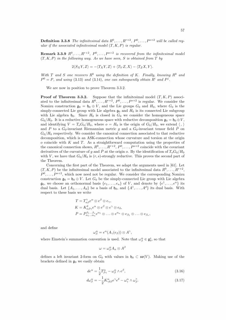
57

Definition 3.3.8 The infinitesimal data R0, . . . , Rr+2, P 0, . . . , P s+2 will be called reg-ular if the associated infinitesimal model (T,K, P ) is regular.

Remark 3.3.9 R0, . . . , Rr+2, P 0, . . . , P s+2 is recovered from the infinitesimal model(T,K, P ) in the following way. As we have seen, S is obtained from T by

2〈SXY,Z〉 = −〈TXY,Z〉+ 〈TY Z,X〉 − 〈TZX,Y 〉.

With T and S one recovers R0 using the definition of K. Finally, knowing R0 andP 0 = P , and using (3.13) and (3.14), one can subsequently obtain Ri and P j.

We are now in position to prove Theorem 3.3.2.

Proof of Theorem 3.3.2. Suppose that the infinitesimal model (T,K, P ) associ-ated to the infinitesimal data R0, . . . , Rr+2, P 0, . . . , P s+2 is regular. We consider theNomizu construction g0 = h0 ⊕ V , and the Lie groups G0 and H0, where G0 is thesimply-connected Lie group with Lie algebra g0 and H0 is its connected Lie subgroupwith Lie algebra h0. Since H0 is closed in G0 we consider the homogeneous spaceG0/H0. It is a reductive homogeneous space with reductive decomposition g0 = h0⊕V ,and identifying V = ToG0/H0, where o = H0 is the origin of G0/H0, we extend 〈 , 〉and P to a G0-invariant Riemannian metric g and a G0-invariant tensor field P onG0/H0 respectively. We consider the canonical connection associated to that reductivedecomposition, which is an ASK-connection whose curvature and torsion at the origino coincide with K and T . As a straightforward computation using the properties ofthe canonical connection shows, R0, . . . , Rr+2, P 0, . . . , P s+2 coincide with the covariantderivatives of the curvature of g and P at the origin o. By the identification of ToG0/H0

with V , we have that G0/H0 is (r, s)-strongly reductive. This proves the second part ofthe Theorem.

Concerning the first part of the Theorem, we adapt the arguments used in [61]. Let(T,K, P ) be the infinitesimal model associated to the infinitesimal data R0, . . . , Rr+2,P 0, . . . , P s+2, which now need not be regular. We consider the corresponding Nomizuconstruction g0 = h0 ⊕ V . Let G0 be the simply-connected Lie group with Lie algebrag0, we choose an orthonormal basis e1, . . . , en of V , and denote by e1, . . . , en itsdual basis. Let A1, . . . , Ad be a basis of h0, and A1, . . . , Ad its dual basis. Withrespect to these basis we write

T = T γαβeα ⊗ eβ ⊗ eγ ,

K = Kδαβγe

α ⊗ eβ ⊗ eγ ⊗ eδ,P = P β1...βv

α1...αueα1 ⊗ . . .⊗ eαu ⊗ eβ1

⊗ . . .⊗ eβv ,

and defineωαβ = eα(Aγ(eβ))⊗Aγ ,

where Einstein’s summation convention is used. Note that ωαβ ∈ g∗0, so that

ω = ωαβAα ⊗Aβ

defines a left invariant 2-form on G0 with values in h0 ⊂ so(V ). Making use of thebrackets defined in g0 we easily obtain

deα =1

2Tαβγ − ωαβ ∧ eβ , (3.16)

dωαβ = −1

2Kαγδβe

γeδ − ωαγ ∧ ωγβ . (3.17)

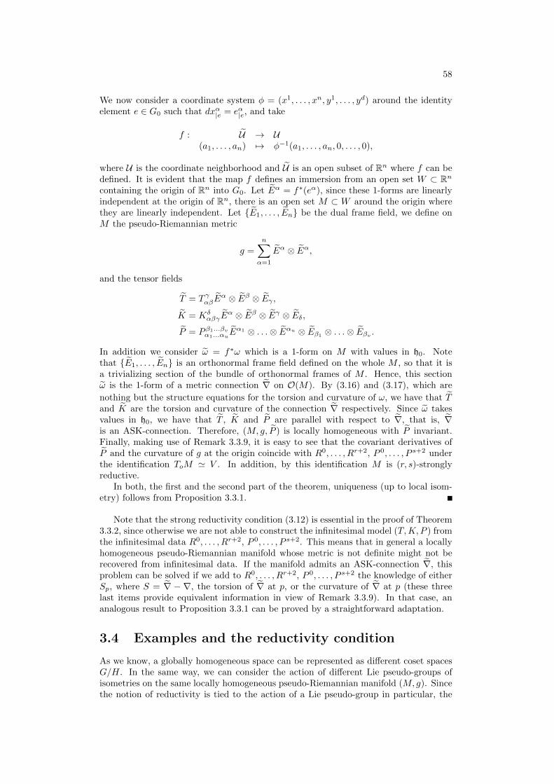
58

We now consider a coordinate system φ = (x1, . . . , xn, y1, . . . , yd) around the identityelement e ∈ G0 such that dxα|e = eα|e, and take

f : U → U(a1, . . . , an) 7→ φ−1(a1, . . . , an, 0, . . . , 0),

where U is the coordinate neighborhood and U is an open subset of Rn where f can bedefined. It is evident that the map f defines an immersion from an open set W ⊂ Rncontaining the origin of Rn into G0. Let Eα = f∗(eα), since these 1-forms are linearlyindependent at the origin of Rn, there is an open set M ⊂ W around the origin wherethey are linearly independent. Let E1, . . . , En be the dual frame field, we define onM the pseudo-Riemannian metric

g =

n∑α=1

Eα ⊗ Eα,

and the tensor fields

T = T γαβEα ⊗ Eβ ⊗ Eγ ,

K = KδαβγE

α ⊗ Eβ ⊗ Eγ ⊗ Eδ,

P = P β1...βvα1...αuE

α1 ⊗ . . .⊗ Eαu ⊗ Eβ1 ⊗ . . .⊗ Eβv .

In addition we consider ω = f∗ω which is a 1-form on M with values in h0. Notethat E1, . . . , En is an orthonormal frame field defined on the whole M , so that it isa trivializing section of the bundle of orthonormal frames of M . Hence, this sectionω is the 1-form of a metric connection ∇ on O(M). By (3.16) and (3.17), which are

nothing but the structure equations for the torsion and curvature of ω, we have that Tand K are the torsion and curvature of the connection ∇ respectively. Since ω takesvalues in h0, we have that T , K and P are parallel with respect to ∇, that is, ∇is an ASK-connection. Therefore, (M, g, P ) is locally homogeneous with P invariant.Finally, making use of Remark 3.3.9, it is easy to see that the covariant derivatives ofP and the curvature of g at the origin coincide with R0, . . . , Rr+2, P 0, . . . , P s+2 underthe identification ToM ' V . In addition, by this identification M is (r, s)-stronglyreductive.

In both, the first and the second part of the theorem, uniqueness (up to local isom-etry) follows from Proposition 3.3.1.

Note that the strong reductivity condition (3.12) is essential in the proof of Theorem3.3.2, since otherwise we are not able to construct the infinitesimal model (T,K, P ) fromthe infinitesimal data R0, . . . , Rr+2, P 0, . . . , P s+2. This means that in general a locallyhomogeneous pseudo-Riemannian manifold whose metric is not definite might not berecovered from infinitesimal data. If the manifold admits an ASK-connection ∇, thisproblem can be solved if we add to R0, . . . , Rr+2, P 0, . . . , P s+2 the knowledge of eitherSp, where S = ∇ − ∇, the torsion of ∇ at p, or the curvature of ∇ at p (these threelast items provide equivalent information in view of Remark 3.3.9). In that case, ananalogous result to Proposition 3.3.1 can be proved by a straightforward adaptation.

3.4 Examples and the reductivity condition

As we know, a globally homogeneous space can be represented as different coset spacesG/H. In the same way, we can consider the action of different Lie pseudo-groups ofisometries on the same locally homogeneous pseudo-Riemannian manifold (M, g). Sincethe notion of reductivity is tied to the action of a Lie pseudo-group in particular, the

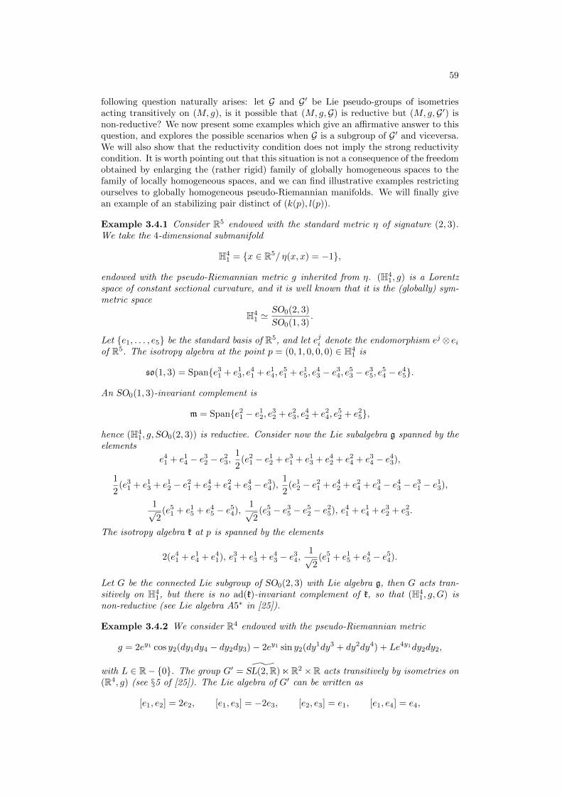
59

following question naturally arises: let G and G′ be Lie pseudo-groups of isometriesacting transitively on (M, g), is it possible that (M, g,G) is reductive but (M, g,G′) isnon-reductive? We now present some examples which give an affirmative answer to thisquestion, and explores the possible scenarios when G is a subgroup of G′ and viceversa.We will also show that the reductivity condition does not imply the strong reductivitycondition. It is worth pointing out that this situation is not a consequence of the freedomobtained by enlarging the (rather rigid) family of globally homogeneous spaces to thefamily of locally homogeneous spaces, and we can find illustrative examples restrictingourselves to globally homogeneous pseudo-Riemannian manifolds. We will finally givean example of an stabilizing pair distinct of (k(p), l(p)).

Example 3.4.1 Consider R5 endowed with the standard metric η of signature (2, 3).We take the 4-dimensional submanifold

H41 = x ∈ R5/ η(x, x) = −1,

endowed with the pseudo-Riemannian metric g inherited from η. (H41, g) is a Lorentz

space of constant sectional curvature, and it is well known that it is the (globally) sym-metric space

H41 '

SO0(2, 3)

SO0(1, 3).

Let e1, . . . , e5 be the standard basis of R5, and let eji denote the endomorphism ej ⊗ eiof R5. The isotropy algebra at the point p = (0, 1, 0, 0, 0) ∈ H4

1 is

so(1, 3) = Spane31 + e1

3, e41 + e1

4, e51 + e1

5, e43 − e3

4, e53 − e3

5, e54 − e4

5.

An SO0(1, 3)-invariant complement is

m = Spane21 − e1

2, e32 + e2

3, e42 + e2

4, e52 + e2

5,

hence (H41, g,SO0(2, 3)) is reductive. Consider now the Lie subalgebra g spanned by the

elements

e41 + e1

4 − e32 − e2

3,1

2(e2

1 − e12 + e3

1 + e13 + e4

2 + e24 + e3

4 − e43),

1

2(e3

1 + e13 + e1

2 − e21 + e4

2 + e24 + e4

3 − e34),

1

2(e1

2 − e21 + e4

2 + e24 + e3

4 − e43 − e3

1 − e13),

1√2

(e51 + e1

5 + e45 − e5

4),1√2

(e53 − e3

5 − e52 − e2

5), e41 + e1

4 + e32 + e2

3.

The isotropy algebra k at p is spanned by the elements

2(e41 + e1

4 + e41), e3

1 + e13 + e4

3 − e34,

1√2

(e51 + e1

5 + e45 − e5

4).

Let G be the connected Lie subgroup of SO0(2, 3) with Lie algebra g, then G acts tran-sitively on H4

1, but there is no ad(k)-invariant complement of k, so that (H41, g,G) is

non-reductive (see Lie algebra A5∗ in [25]).

Example 3.4.2 We consider R4 endowed with the pseudo-Riemannian metric

g = 2ey1 cos y2(dy1dy4 − dy2dy3)− 2ey1 sin y2(dy1dy3 + dy2dy4) + Le4y1dy2dy2,

with L ∈ R− 0. The group G′ = ˜SL(2,R)nR2 ×R acts transitively by isometries on(R4, g) (see §5 of [25]). The Lie algebra of G′ can be written as

[e1, e2] = 2e2, [e1, e3] = −2e3, [e2, e3] = e1, [e1, e4] = e4,

60

[e1, e5] = −e5, [e2, e5] = e4, [e3, e4] = e5,

with respect to some basis e1, . . . , e6, which is the Lie algebra B3 in [25]. In additionit is the full isometry algebra of (R4, g) and can be realized by the complete Killing vectorfields

Y1 = cos(2y2)∂y1− sin(2y2)∂y2

+ y3∂y3− y4∂y4

,

Y2 =1

2sin(2y2)∂y1 + cos2(y2)∂y2 + y3∂y4 ,

Y3 =1

2sin(2y2)∂y1

− sin2(y2)∂y2+ y4∂y3

,

Y4 = ∂y4,

Y5 = −∂y3,

Y6 = ey1 cos(y2)∂y3+ ey1 sin(y2)∂y4

.

The isotropy algebra at (0, 0, 0, 0) ∈ R4 is Spane3, e5+e6. As stated in [25], (R4, g,G′)is non-reductive. We take the subalgebra g = Spane1, e2, e4, e5, e6. Making use of thedistribution generated by the corresponding Killing vector fields we see that the actionof the connected Lie subgroup G ⊂ G′ with Lie algebra g is transitive. The isotropyalgebra at (0, 0, 0, 0) is k = Spane5 + e6, and m = Spane1, e2, e4, e5 is an Ad(K)-invariant complement, where K ⊂ G is the isotropy group with respect to the action ofG at (0, 0, 0, 0). Therefore (R4, g,G) is reductive. On the other hand we can check that(R4, g) is not strongly reductive. In this case, since there is no extra geometric structure,the complex of filtrations reduces to

so(TpM) ⊃ g(p, 0) ⊃ g(p, 1) ⊃ . . .

A simple computation shows that the only non-zero component of the curvature isR∂y1∂y2∂y1∂y2 = −3Le4y1 , and ∇R = 0. We take p = (0, 0, 0, 0) and L = 1 for thesake of simplicity, so that the filtration actually is

so(TpM) ⊃ g(p, 0) = g(p, 1),

where

so(TpM) =

−e 2(b− c) b 0f 2a a c

2(d− f) 0 −2a 2(b− c)0 2(d− f) d e

/ a, b, c, d, e, f ∈ R

,

g(p, 0) = A ∈ so(TpM)/ e = 2a, f = d .

It is easy to check that g(p, 0) does not admit any complement n invariant by the adjointaction of g(p, 0), hence (R4, g) cannot be strongly reductive.

We finally exhibit an example of a locally homogeneous pseudo-Kahler manifold withan stabilizing pair distinct form (k, l), where as usual (k, l) are the first integers suchthat g(p, k) = g(p, k + 1) and p(p, l) = p(p, l + 1).

Example 3.4.3 Consider the space C2 with complex coordinates (w, z). We take M =C2 − ||w|| = 0 with the standard complex structure J and the pseudo-Riemannianmetric

g = dw1dz1 + dw2dz2 + b(dw1dw1 + dw2dw2),

where w = w1 + iw2, z = z1 + iz2, and b is a function depending on w1 and w2

and satisfying ∆b = R0

||w||4 for some R0 6= 0. This manifold is locally homogeneous

61

since it admits an ASK-connection (see Proposition 5.2.7 in Chapter 5). Let θ =− 1||w||2 (w1dw1 + w2dw2), the curvature tensor and its first covariant derivative are

R =1

2

R0

||w||4(dw1 ∧ dw2 ⊗ dw1 ∧ dw2), ∇R = 4θ ⊗R.

We set R0 = 2 and take the point p = (−1, 0, 0, 0), so that

Rp = dw1 ∧ dw2 ⊗ dw1 ∧ dw2, ∇Rp = 4dw1 ⊗Rp,

∇2Rp = (20dw1 ⊗ dw1 − 4dw2 ⊗ dw2)⊗Rp.

On the other hand, Jp is the standard complex structure of C2 and ∇Jp = 0 since themanifold is pseudo-Kahler. A straightforward computations thus shows that the complexof filtrations is

so(R4)6 ⊃ g(p, 0)2 ⊃ g(p, 1)1 = g(p, 2)1

∪ || || ||p(p, 0)4 ⊃ h(p, 0, 0)2 ⊃ h(p, 1, 0)1 = h(p, 2, 0)1

|| || || ||p(p, 1)4 ⊃ h(p, 0, 1)2 ⊃ h(p, 1, 1)1 = h(p, 2, 1)1,

where superindices indicate dimension. We have that (k, l) = (1, 0), but (r, s) = (1,−1)is a stabilizing pair.

Chapter 4

Classification of homogeneousstructures

In previous sections we have seen how AS-connections and ASK-connections are a usefultool for studying homogeneous and locally homogeneous spaces. For instance, for glob-ally homogeneous manifolds, the presence of an AS-connection (or an ASK-connection)characterizes reductive spaces, and provides a representation as a coset space. For thatreason, a classification of the possible AS-connections or ASK-connections can help notonly to understand different coset representations of the same homogeneous space, butalso to shade light to the structure of the vast world of homogeneous and locally homo-geneous spaces. A very efficient way to aboard this problem is to classify the possiblehomogeneous structures S, which are essentially the torsion of the corresponding AS orASK-connection. The advantage of this approach is that the work can be completelydone at an algebraic level (similar to how intrinsic torsion is studied in Riemannian ge-ometry), and some tools like representation theory may apply (see [26]). In this chapterwe show a procedure to classify homogeneous structures associated to AS-connectionsand ASK-connections whose underlying geometric structure is integrable. We then willapply that procedure to the geometric structures that will be treated in subsequentchapters.

4.1 General procedure

Let S be a homogeneous structure on (M, g) associated to an AS-connection ∇, we willindistinctively refer by S to the (1, 2)-tensor field or the metric equivalent (0, 3)-tensorfield, that is,

SXY Z = g(SXY,Z).

This convention will be used hereafter. Let ∇ be the Levi-Civita connection of g,equation ∇g = 0 becomes

0 = ∇g = ∇g − S · g = −S · g = 0.

This means that for every X ∈ X(M) we have SX · g = 0, where SX acts as a derivationon the tensor algebra, that is,

SXY Z + SXZY = 0, X, Y, Z ∈ X(M).

Let x ∈ M , choosing an orthonormal basis of TxM we can consider the vector spaceV = Rm endowed with the standard symmetric bilinear form 〈 , 〉 of signature (r, s)as a model of (TxM, gx). We take the space of tensors S(V ) ⊂ ⊗3V ∗ with the samesymmetries as the homogeneous structure S, that is

S(V ) = S ∈ ⊗3V ∗/ SXY Z + SXZY = 0.

63

64

As a vector space S(V ) is isomorphic to V ∗ ⊗ ∧2V ∗, and carries a non-degeneratesymmetric bilinear form defined by

〈S, S′〉 =

m∑i,j,k=1

εiεjεkSeiejekS′eiejek

,

where e1, . . . , em is any othonormal basis of (V, 〈 , 〉), and εi = 〈ei, ei〉. Furthermore,there is a natural left action of the orthogonal group O(r, s) given by

(A · S)XY Z = SA−1XA−1Y A−1Z , A ∈ O(V ), X, Y, Z ∈ V,

turning S(V ) into a O(r, s)-module. Identifying ∧2V ∗ with so(r, s), we have that S(V ) 'V ∗ ⊗ so(r, s), and the action of O(r, s) is seen as the tensor product of the standardrepresentation and the adjoint representation.

Suppose that there is a geometric structure on (M, g) defined by a tensor field P (thecase of geometric structures given by more than one tensor field is analogous), and thatS is associated to an ASK-connection. Assume moreover that this geometric structureis integrable. Recall that this means that the holonomy of g at x ∈ M can be seenas a subgroup of the stabilizer Hx of Px inside O(TxM), or equivalently that ∇P = 0.

Equation ∇P = 0 thus becomes

0 = ∇P − S · P = −S · P,

whence (Sx)X can be seen as an element of the Lie algebra hx of H(x) for every X ∈TxM . With the help of an orthonormal basis of TxM , we consider a tensor field P0 on Vas the model of Px, and denote by H and h the stabilizer of P0 inside O(r, s) and its Liealgebra respectively. The space of tensors on V with the same symmetries as S is thusidentified with V ∗⊗h ⊂ S(V ). The natural action of H as a subgroup of O(r, s) restrictsto V ∗⊗h, as it is just the tensor product of the standard and the adjoint representation.This turns V ∗ ⊗ h into an H-module. Note that the action of H is orthogonal withrespect to the bilinear form 〈 , 〉 on S(V ). One of the main differences between theRiemannian and the pseudo-Riemannian cases is that for pseudo-Riemannian metrics〈 , 〉 need not be definite. The H-module V ∗⊗h can be thus decomposed into the directsum of mutually orthogonal indecomposable H-submodules. As it happened with theholonomy representation, if g is definite we can assure that V ∗⊗h is decomposable intothe direct sum of irreducible H-submodules. This is also the case when H is semisimple(for instance all the groups appearing in Berger’s list are semisimple).

Assume now that we have decomposed V ∗⊗h into H-submodules W 1, . . . ,W l, thatis

V ∗ ⊗ h = W 1 ⊕ . . .⊕W l.

For every x ∈ M , this gives a decomposition of the Hx-module T ∗xM ⊗ hx into Hx-submodules W 1

x , . . . ,Wlx, that is

T ∗xM ⊗ hx = W 1x ⊕ . . .⊕W l

x.

Proposition 4.1.1 Let S be a homogeneous structure. If Sx belongs to the submoduleW ix for some i = 1, . . . , l at a point x ∈M , then it belongs to the submodule W i

y at everypoint y ∈M .

Proof. Since (M, g, P ) is at least locally homogeneous with P invariant, there is a linearisometry φ : TxM → TyM preserving P and S. Taking orthonormal basis we identifyTxM and TyM with V , so that φ turns into an element of the group H. This impliesthat the induced transformation of V ∗ ⊗ h preserves the H-submodules W 1, . . . ,W l.Since S is also invariant by φ we have that Sx ∈W i

x if and only if Sy ∈W iy.

65

The previous Proposition shows that a certain decomposition of V ∗ ⊗ h into H-submodules induces a classification of homogeneous structures, classification which isthus of purely algebraic nature. That decomposition can be done for every particularcase in two ways: using representation theory, and by real tensors. For the representationtheory approach we will make use of the techniques in [53], which provide a method todecompose tensor products of representations of Lie groups (see also [5, 7, 64]).

4.2 Some classifications

In this section we apply the classification procedure to some integrable geometric struc-tures. The classifications obtained for each case will lead to the notion of homogeneousstructures of linear type, which will be a central object of study in the rest of this thesis.During this section all sums of vector spaces are direct sums.

4.2.1 Homogeneous pseudo-Riemannian structures

We consider homogeneous structures S on pseudo-Riemannian manifolds (M, g) withoutconsidering any geometric structure on them. In other words we assume that S is asso-ciated to just an AS-connection and thus only takes into account (2.1). Such structureswill be simply called homogeneous pseudo-Riemannian structures. In view of the previ-ous section, in order to classify this kind of homogeneous structures we will decomposethe O(r, s)-module S(V ) into irreducible submodules. Suppose that m = dimM ≥ 3.From the general representation theory for the orthonormal group (see [5, 64]) we havethe decomposition

V ∗ ⊗ ∧2V ∗ ' V ∗ ⊗W ⊗ ∧3V ∗,

where W is the irreducible representation of O(r, s) associated to Young element id +(12) − (23) − (132). We now show the explicit expression of the tensors of these sub-modules. Consider the equivariant map

c12 : S(V ) → V ∗

S 7→ c12(S)(Z) =∑mi=1 ε

iSeieiZ ,

where ei is any orthonormal basis of V and εi = 〈ei, ei〉. The subspace ker(c12) isnon-degenerate with respect to the symmetric bilinear form on S(V ), and its orthogonalcomplement is

ker(c12)⊥ = S ∈ S(V )/ SXY Z = 〈X,Y 〉ϕ(Z)− 〈X,Z〉ϕ(Y ), ϕ ∈ V ∗.

We now take the equivariant map

L : S(V ) → S(V )S 7→ L(S) = SXYZ

SXY Z .

This map satisfies L2 = 3L so that it is diagonalizable with real eigenvalues 0 and 3.The corresponding eigenspaces

S0(V ) = S ∈ V/ SXYZ

SXY Z = 0

S3(V ) = S ∈ S(V )/ SXY Z + SY XZ = 0

are mutually orthogonal and invariant by O(r, s). It is easy to check that S3(V ) ⊂ker(c12) and ker(c12)⊥ ⊂ S0(V ). We set S1(V ) = ker(c12)⊥, S2(V ) = S0(V )∩ker(c12),and S3(V ) = S3(V ).

66

Proposition 4.2.1 ([60, 31]) If m ≥ 3, then the space S(V ) decomposes into irre-ducible and mutually orthogonal O(r, s)-submodules as

S(V ) = S1(V ) + S2(V ) + S3(V ).

If m = 2, then S(V ) = S1(V ).

Let S denote the set of homogeneous pseudo-Riemannian structures, we thus obtainthe following classification:

S1 =S ∈ S / SXY Z = g(X,Y )ϕ(Z)− g(X,Z)ϕ(Y ), ϕ ∈ Ω1(M)

S2 =

S ∈ S / S

XYZ

SXY Z = 0, c12(S) = 0

S3 =S ∈ S / SXY Z + SY XZ = 0

Taking into account that

dimS1(V ) = m, dimS2(V ) =m(m− 2)(m+ 2)

3, dimS3(V ) =

(m3

),

we note that homogeneous pseudo-Riemannian structures in the class S1 are sectionsof a vector bundle whose rank grows linearly with the dimension of the manifold. Thismotivates the following definition.

Definition 4.2.2 A homogeneous pseudo-Riemannian structure is called of linear typeif it belongs to the class S1.

It is easy to see that a homogeneous pseudo-Riemanian structure of linear type seenas a (1, 2)-tensor field takes the form

SXY = g(X,Y )ξ − g(Y, ξ)X, (4.1)

for some vector field ξ ∈ X(M). In addition, if S takes the previous form then Ambrose-Singer equations are equivalent to

∇R = 0, ∇ξ = 0.

As we are working with metrics with signature a subclassification of this kind of struc-tures will be needed.

Definition 4.2.3 A homogeneous pseudo-Riemannian structure of linear type S definedby the vector field ξ is called

1. non-degenerate if g(ξ, ξ) = 0,

2. degenerate if g(ξ, ξ) = 0.

4.2.2 Homogeneous pseudo-Kahler structures

We consider homogeneous structures S on pseudo-Kahler manifolds (M, g, J), satisfyingAmbrose-Singer-Kiricenko equtions, that is

∇g = 0, ∇R = 0, ∇S = 0, ∇J = 0.

Such structures will be called homogeneous pseudo-Kahler structures. In this case thestabilizer of the complex structure inside O(r, s) is the corresponding unitary groupU(p, q), where 2p = r and 2q = s. We thus decompose the U(p, q)-module K(V ) =

67

V ∗ ⊗ u(p, q) ⊂ S(V ) into irreducible submodules. As a representation of U(p, q), thespace K(V ) is isomorphic to the tensor product of the standard representation and theadjoint representation of U(p, q). Suppose that m = dimM ≥ 6. Following [53] weadopt the notation JΛk,lK ⊗ C = Λk,l + Λl,k, [Λk,k] ⊗ C = Λk,k, where Λk,l denotesthe space of forms of type (k, l) on V ⊗ C with respect to J . The standard and theadjoint representation can thus be written as JΛ0,1K and R + [Λ1,1

0 ] respectively, wherethe subindex 0 denotes the primitive part with respect to the symplectic form associatedto J . As complex representations we have [26]

Λ1,0 ⊗ Λ1,10 ' Λ1,0 + Λ2,1

0 + S2,10 ,

where S2,10 is the kernel of the anti-symmetrization Λ1,0 ⊗ Λ1,1

0 → Λ2,1. We obtain

V ∗ ⊗ u(p, q) ' JΛ0,1K⊗(R+ [Λ1,1

0 ])' JΛ0,1K + JΛ0,1K + JΛ2,1

0 K + JS2,10 K.

We now give the explicit expression of the tensors in these submodules. Consider theequivariant map

L : K(V ) → K(V )S 7→ L(S)XY Z = 1

2 (SY ZX + SZXY + SJY JZX + SJZXJY ) ,

which is also orthogonal with respect to the symmetric bilinear form inherited fromS(V ). As a simple computation shows L2 = Id, so that L is diagonalizable witheigenvalues ±1. The corresponding eigenspaces K±1(V ) are mutually orthogonal andinvariant by U(p, q). Taking the contraction c12, each eigenspace splits in two mutuallyorthogonal submodules

K±1(V ) = K±1(V ) ∩ ker(c12) +K±1(V ) ∩ ker(c12)⊥.

We set K1 = K1(V )∩ker(c12), K2(V ) = K1(V )∩ker(c12)⊥, K3(V ) = K−1(V )∩ker(c12),and K4(V ) = K−1(V ) ∩ ker(c12)⊥.

Proposition 4.2.4 ([1, 8]) If m ≥ 6, the space K(V ) is decomposed into mutuallyorthogonal and irreducible U(p, q)-submodules as

K(V ) = K1(V ) +K2(V ) +K3(V ) +K4(V ),

where

K1(V ) =S ∈ K(V ) / SXY Z =

1

2(SY ZX + SZXY + SJY JZX + SJZXJY ),

c12(S) = 0,

K2(V ) =S ∈ K(V ) / SXY Z = 〈X,Y 〉θ1(Z)− 〈X,Z〉θ1(Y ) + 〈X, JY 〉θ1(JZ)

− 〈X,JZ〉θ1(JY )− 2〈JY, Z〉θ1(JX), θ1 ∈ V ∗,

K3(V ) =S ∈ K(V ) / SXY Z = −1

2(SY ZX + SZXY + SJY JZX + SJZXJY ),

c12(S) = 0,

K4(V ) =S ∈ K(V ) / SXY Z = 〈X,Y 〉θ2(Z)− 〈X,Z〉θ2(Y ) + 〈X, JY 〉θ2(JZ)

− 〈X,JZ〉θ2(JY ) + 2〈JY, Z〉θ2(JX), θ2 ∈ V ∗.

If m = 4 then K(V ) = K2(V ) +K3(V ) +K4(V ). If m = 2 then K(V ) = K4(V ).

68

Taking into account that

dimK1(V ) = n(n+ 1)(n− 2), dimK2(V ) = dimK4(V ) = 2n,

dimK3(V ) = n(n− 1)(n+ 2),

where m = 2n, we note that homogeneous pseudo-Kahler structures in the composedclass K2 +K4 are sections of a vector bundle whose rank grows linearly with the dimen-sion of the manifold. This motivates the following definition.

Definition 4.2.5 A homogeneous pseudo-Kahler structure is called of linear type if itbelongs to the class K2 +K4.

It is easy to see that a homogeneous pseudo-Kahler structure of linear type seen asa (1, 2)-tensor field takes the form

SXY = g(X,Y )ξ − g(Y, ξ)X − g(X, JY )Jξ + g(JY, ξ)JX − 2g(JX, ζ)JY, (4.2)

for some vector fields ξ, ζ ∈ X(M). In addition, if S takes the previous form, thenAmbrose-Singer-Kiricenko equations are equivalent to

∇R = 0, ∇ξ = 0, ∇ζ = 0. (4.3)

As we are working with metrics with signature, a subclassification of this kind of struc-tures will be needed.

Definition 4.2.6 A homogeneous pseudo-Kahler structure of linear type S defined bythe vector fields ξ and ζ is called

1. non-degenerate if g(ξ, ξ) = 0,

2. degenerate if g(ξ, ξ) = 0.

3. strongly degenerate if g(ξ, ξ) = 0 and ζ = 0.

4.2.3 Homogeneous para-Kahler structures

We consider homogeneous structures S on para-Kahler manifolds (M, g, J), satisfyingAmbrose-Singer-Kiricenko equations, that is

∇g = 0, ∇R = 0, ∇S = 0, ∇J = 0.

Such structures will be called homogeneous para-Kahler structures. In this case the sta-bilizer of the para-complex structure J inside O(r, s) is the para-unitary group Gl(n,R),where dimM = m = 2n. We thus have to decompose the Gl(n,R)-module

PK(V ) = V ∗ ⊗ gl(n,R) ⊂ S(V )

into irreducible submodules. Note that V is an indecomposable but reducible represen-tation of Gl(n,R) since there are two invariant maximal isotropic and complementarysubspaces of V . These subspaces are exactly the eigenspaces V+ and V− correspondingto the eigenvalues ±1 of J , and they have the same dimension. Taking V + and V − thedual spaces of V+ and V− respectively, we have

V ∗ ⊗ gl(n,R) ' V + ⊗ gl(n,R) + V − ⊗ gl(n,R).

We denote Λk,−l = ∧kV + ⊗ ∧lV −. Under the identification so(r, s) ' ∧2V ∗ we havethat gl(n,R) is identified with Λ1,−1. Let ω ∈ Λ1,−1 be the symplectic form associatedto J , we decompose Λ1,−1 = Rω + Λ1,−1

0 . Hence

V + ⊗ gl(n,R) ' V + ⊗ R+ V + ⊗ Λ1,−10 .

69

On the other handV + ⊗ Λ1,−1

0 ' V + + Λ2,−10 + S2,−1

0 ,

where S2,−10 is the kernel of the anti-symmetrization V + ⊗ Λ1,−1

0 → Λ2,−1, and Λ2,−10

is the primitive part of Λ2,−1 with respect to ω. Since the complexification of gl(n,R)is isomorphic to gl(n,C), which coincides with the complexification of u(p, q), the rep-resentation theory for gl(n,R) and u(p, q) is analogous. Using this fact it is easy to seethat the submodules Λ2,−1

0 and S2,−10 are irreducible. A decomposition of V − ⊗ Λ1,−1

is carried out in a similar way. Summarizing we obtain

V ∗ ⊗ gl(n,R) ' 2V + + 2V − + Λ2,−10 + Λ1,−2

0 + S2,−10 + S1,−2

0 .

On the other hand, we consider the equivariant map

L : K(V ) → K(V )S 7→ L(S)XY Z = 1

2 (SY ZX + SZXY − SJY JZX − SJZXJY ) ,

which is also orthogonal with respect to the symmetric bilinear form inherited fromS(V ). As a simple computation shows L2 = Id, so that L is diagonalizable witheigenvalues ±1. The corresponding eigenspaces W±1(V ) are mutually orthogonal andinvariant by Gl(n,R). Taking now the contraction c12, each eigenspace splits into twomutually orthogonal submodules

W±1 =W±1 ∩ ker(c12) +W±1 ∩ ker(c12)⊥.

We set U1 = W1 ∩ ker(c12), U2 = W1 ∩ ker(c12)⊥, U3 = W−1 ∩ ker(c12), and U4 =W−1∩ker(c12)⊥. The submodules U1, . . . ,U4 are indecomposable but reducible. Indeed,the splitting V = V+ + V− induce decompositions Ui = U+

i + U−i where

U+i =

S ∈ Ui/ SX−Y Z = 0, X− ∈ V−

,

U−i =S ∈ Ui/ SX+Y Z = 0, X+ ∈ V+

.

We setPK1(V ) = U+

1 , PK2(V ) = U+2 , PK3(V ) = U+

3 , PK4(V ) = U+4 ,

PK5(V ) = U−1 , PK6(V ) = U−2 , PK7(V ) = U−3 , PK8(V ) = U−4 .

Proposition 4.2.7 ([30]) If m ≥ 6, the space PK(V ) is decomposed into irreducibleGl(n,R)-submodules as

PK(V ) = PK1(V ) + PK2(V ) + PK3(V ) + PK4(V )

+ PK5(V ) + PK6(V ) + PK7(V ) + PK8(V ),

where

PK1(V ) =S ∈ PK(V ) / SXY Z =

1

2(SY ZX + SZXY − SJY JZX − SJZXJY ),

c12(S) = 0, SX−Y Z = 0, X− ∈ V−,

PK2(V ) =S ∈ PK(V ) / SXY Z = 〈X,Y 〉θ1(Z)− 〈X,Z〉θ1(Y )− 〈X, JY 〉θ1(JZ)

+ 〈X,JZ〉θ1(JY ) + 2〈JY, Z〉θ1(JX), θ1 ∈ V +,

PK3(V ) =S ∈ PK(V ) / SXY Z = −1

2(SY ZX + SZXY − SJY JZX − SJZXJY ),

c12(S) = 0, SX−Y Z = 0, X− ∈ V−,

PK4(V ) =S ∈ PK(V ) / SXY Z = 〈X,Y 〉θ2(Z)− 〈X,Z〉θ2(Y )− 〈X, JY 〉θ2(JZ)

+ 〈X,JZ〉θ2(JY )− 2〈JY, Z〉θ2(JX), θ2 ∈ V +,

70

and PK5, . . . ,PK8 are obtained from PK1, . . . ,PK4 interchanging + by −. If m = 4then

PK(V ) = PK2(V ) + PK3(V ) +K4(V ) + PK6(V ) + PK7(V ) +K8(V ).

If m = 2 then K(V ) = PK4(V ) + PK8(V ).

Taking into account that

dimPK1(V ) = dimPK5(V ) =n(n+ 1)(n− 2)

2,

dimPK3(V ) = dimPK7(V ) =n2(n+ 1)

2− n,

dimPK2(V ) = dimPK4(V ) = dimPK6(V ) = dimPK8(V ) = n,

we note that homogeneous para-Kahler structures in the composed class PK2 +PK4 +PK6+PK8 are sections of a vector bundle whose rank grows linearly with the dimensionof the manifold. This motivates the following definition.

Definition 4.2.8 A homogeneous para-Kahler structure is called of linear type if itbelongs to the class PK2 + PK4 + PK6 + PK8.

It is easy to see that a homogeneous para-Kahler structure of linear type seen as a(1, 2)-tensor field takes the form

SXY = g(X,Y )ξ − g(Y, ξ)X + g(X, JY )Jξ − g(JY, ξ)JX − 2g(JX, ζ)JY, (4.4)

for some vector fields ξ, ζ ∈ X(M). In addition, if S takes the previous form, thenAmbrose-Singer-Kiricenko equations are equivalent to

∇R = 0, ∇ξ = 0, ∇ζ = 0. (4.5)

As the underlying metric g is not definite, a subclassification of this kind of structureswill be needed.

Definition 4.2.9 A homogeneous para-Kahler structure of linear type S defined by thevector fields ξ and ζ is called

1. non-degenerate if g(ξ, ξ) = 0,

2. degenerate if g(ξ, ξ) = 0.

3. strongly degenerate if g(ξ, ξ) = 0 and ζ = 0.

4.2.4 Homogeneous pseudo-quaternion Kahler structures

Let (M, g,Q) be a pseudo-quaternion Kahler manifold, we consider homogeneous struc-tures S satisfying Ambrose-Singer-Kiricenko equations, that is

∇g = 0, ∇R = 0, ∇S = 0, ∇Ω = 0.

Such structures will be called homogeneous pseudo-quaternion Kahler structures. In thiscase, the stabilizer of the 4-form Ω inside O(r, s) is Sp(p, q)Sp(1), where 4p = r and 4q =s. We thus decompose the Sp(p, q)Sp(1)-moduleQK(V ) = V ∗⊗(sp(p, q)+sp(1)) ⊂ S(V )into irreducible submodules. Suppose that m = dimM ≥ 8. Let n = p + q, following[16] we denote by E = C2n and H = C2 the standard representations of Sp(p, q) andSp(1) respectively. The product of the quaternionic structures on E and H gives realstructures on tensor products of E and H, and we denote the real part with respect to

71

these real structures with brackets. For the sake of simplicity we will omit some tensorproducts and write EH for E ⊗ H, etc. The standard representation of Sp(p, q)Sp(1)is thus V = [EH], and the adjoint representation is isomorphic to [S2E] + [S2H]. Wethus have

V ∗ ⊗ (sp(p, q) + sp(1)) ' [EH]⊗ ([S2E] + [S2H]) ' [EH]⊗ [S2E] + [EH]⊗ [S2H].

As complex representations E and S2E has highest weights (1, 0, . . . , 0) and (2, 0, . . . , 0)respectively. Making use of the techniques in [53] we have the decomposition

(1, 0, . . . , 0)⊗ (2, 0, . . . , 0) ' (2, 1, 0 . . . , 0) + (3, 0, . . . , 0) + (1, 0, . . . , 0)

' K + S3E + E,

where K is the module associated to the irreducible representation with highest weight(2, 1, 0, . . . , 0). In addition, H ⊗S2H ' H +S3H, where H is identified with the kernelof the symmetrization H ⊗S2H → S3H. Summarizing we have the decomposition intoirreducible representations [26]

V ∗ ⊗ (sp(p, q) + sp(1)) = [EH] + [ES2H] + [EH] + [S3EH] + [KH].

We now show the explicit espression of the tensors. The condition ∇Ω is equivalentto

∇XJa =

3∑b=1

dabJb, a = 1, 2, 3, (4.6)

where (dab) is a matrix of 1-forms sitting in sp(1). This implies that

Ja(SXY )− SX(JaY ) =

3∑b=1

cab(X)JbY, a = 1, 2, 3,

where (cab) a matrix of 1-forms sitting in sp(1). Note that (cab) can be obtained as thesp(1)-part of SX ∈ sp(p, q) + sp(1). The symmetries satisfied by a pseudo-quaternionKahler structure are thus

SXY Z =− SXZY , (4.7)

SXJaY JaZ − SX,Y,Z =− πc(X)g(JbY, JaZ) + πb(X)g(JcY, JaZ), (4.8)

for any cyclic permutation (a, b, c) of (1, 2, 3), where π1, π2, π3 are local 1-forms on M ,and Einstein summation convention is used. We take the sum of the three equations

in (4.8), which up to a factor 4 is ΘS =1

2πa ⊗ ωa. Using the left hand sides of (4.8)

one sees that ΘS satisfies (4.7) and (4.8) for the same 1-forms π1, π2, π3 as S. We

now consider the tensor TSXY Z =1

4

(SXY Z +

∑3a=1 SXJaY JaZ

). This tensor satisfies

TSXJaY JaZ − TSXY Z = 0, a = 1, 2, 3, and TS + ΘS = S. We can thus define invariant

subspaces of QK(V )

V =

Θ ∈ QK(V )/ ΘXY Z =

1

2πa(X)〈JaY, Z〉, πa ∈ V ∗, a = 1, 2, 3

V =

T ∈ QK(V )/ TSXJaY JaZ − T

SXY Z = 0, a = 1, 2, 3

,

so thatQK(V ) = V + V.

The kernel of the equivariant map c12 restricted to V gives the space V0 = ker(c12) ⊂ V,on which the symmetric bilinear form inherited from S(V) is non-degenerate. HenceV = V0 + V⊥0 , where

V⊥0 =

Θ ∈ V/Θ = −∑a

(θ Ja)⊗ ωa, θ ∈ V ∗.

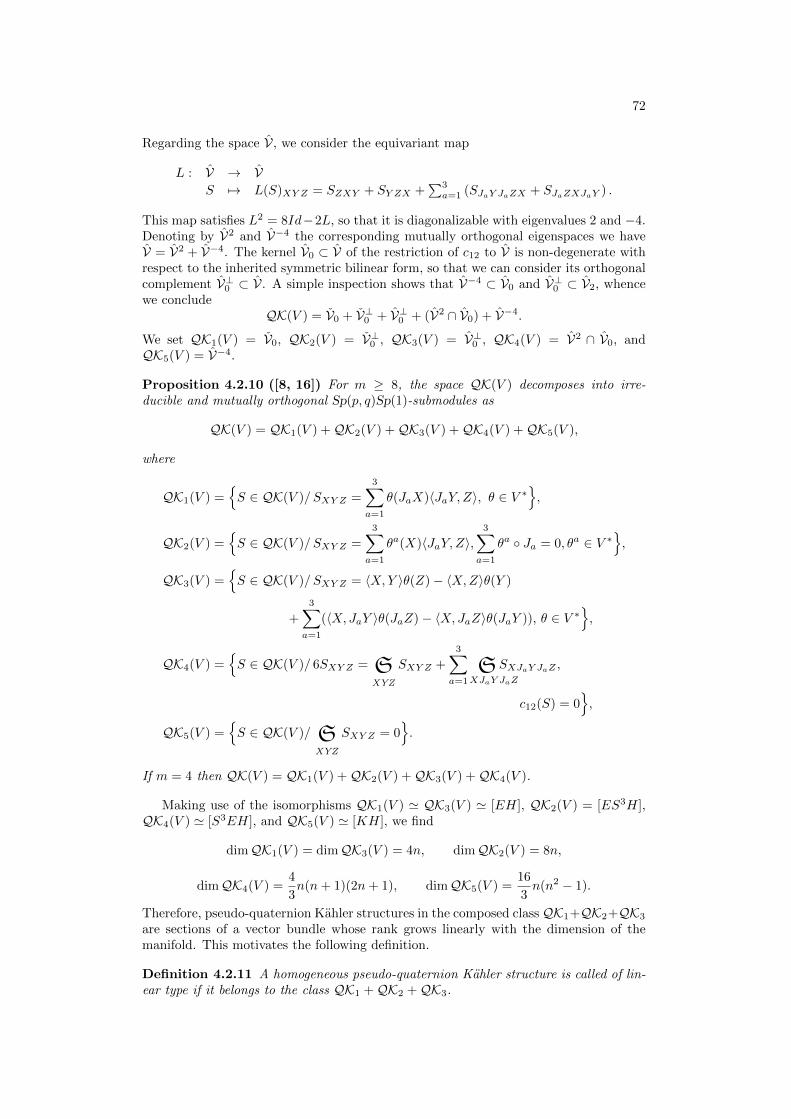
72

Regarding the space V, we consider the equivariant map

L : V → VS 7→ L(S)XY Z = SZXY + SY ZX +

∑3a=1 (SJaY JaZX + SJaZXJaY ) .

This map satisfies L2 = 8Id−2L, so that it is diagonalizable with eigenvalues 2 and −4.Denoting by V2 and V−4 the corresponding mutually orthogonal eigenspaces we haveV = V2 + V−4. The kernel V0 ⊂ V of the restriction of c12 to V is non-degenerate withrespect to the inherited symmetric bilinear form, so that we can consider its orthogonalcomplement V⊥0 ⊂ V. A simple inspection shows that V−4 ⊂ V0 and V⊥0 ⊂ V2, whencewe conclude

QK(V ) = V0 + V⊥0 + V⊥0 + (V2 ∩ V0) + V−4.

We set QK1(V ) = V0, QK2(V ) = V⊥0 , QK3(V ) = V⊥0 , QK4(V ) = V2 ∩ V0, andQK5(V ) = V−4.

Proposition 4.2.10 ([8, 16]) For m ≥ 8, the space QK(V ) decomposes into irre-ducible and mutually orthogonal Sp(p, q)Sp(1)-submodules as

QK(V ) = QK1(V ) +QK2(V ) +QK3(V ) +QK4(V ) +QK5(V ),

where

QK1(V ) =S ∈ QK(V )/ SXY Z =

3∑a=1

θ(JaX)〈JaY,Z〉, θ ∈ V ∗,

QK2(V ) =S ∈ QK(V )/ SXY Z =

3∑a=1

θa(X)〈JaY, Z〉,3∑a=1

θa Ja = 0, θa ∈ V ∗,

QK3(V ) =S ∈ QK(V )/ SXY Z = 〈X,Y 〉θ(Z)− 〈X,Z〉θ(Y )

+

3∑a=1

(〈X,JaY 〉θ(JaZ)− 〈X, JaZ〉θ(JaY )), θ ∈ V ∗,

QK4(V ) =S ∈ QK(V )/ 6SXY Z = S

XYZ

SXY Z +

3∑a=1

SXJaY JaZ

SXJaY JaZ ,

c12(S) = 0,

QK5(V ) =S ∈ QK(V )/ S

XYZ

SXY Z = 0.

If m = 4 then QK(V ) = QK1(V ) +QK2(V ) +QK3(V ) +QK4(V ).

Making use of the isomorphisms QK1(V ) ' QK3(V ) ' [EH], QK2(V ) = [ES3H],QK4(V ) ' [S3EH], and QK5(V ) ' [KH], we find

dimQK1(V ) = dimQK3(V ) = 4n, dimQK2(V ) = 8n,

dimQK4(V ) =4

3n(n+ 1)(2n+ 1), dimQK5(V ) =

16

3n(n2 − 1).

Therefore, pseudo-quaternion Kahler structures in the composed classQK1+QK2+QK3

are sections of a vector bundle whose rank grows linearly with the dimension of themanifold. This motivates the following definition.

Definition 4.2.11 A homogeneous pseudo-quaternion Kahler structure is called of lin-ear type if it belongs to the class QK1 +QK2 +QK3.

73

It is easy to see that a homogeneous pseudo-quaternion Kahler structure of lineartype takes the form

SXY = g(X,Y )ξ − g(Y, ξ)X +

3∑a=1

(g(JaY, ξ)JaX − g(X,JaY )Jaξ)

+

3∑a=1

g(X, ζa)JaY, (4.9)

for some vector fields ξ and ζa, a = 1, 2, 3. When working with metrics with signaturewe need the following further definition.

Definition 4.2.12 A homogeneous pseudo-quaternion Kahler structure of linear typedefined by the vector fields ξ and ζa, a = 1, 2, 3, is called

1. non-degenerate if g(ξ, ξ) = 0,

2. degenerate if g(ξ, ξ) = 0.

A homogeneous pseudo-hyper-Kahler structure is a homogeneous structure on apseudo-hyper-Kahler manifold (M, g, J1, J2, J3) satisfying ∇Ja = 0, a = 1, 2, 3. Thisimplies that S satisfies (4.7) and (4.8) with πa = 0 for a = 1, 2, 3. Therefore, the de-composition of HK(V ) = V ∗ ⊗ sp(r, s) can be read in terms of the pseudo-quaternionKahler case. In fact,

HK(V ) = HK1(V ) +HK2(V ) +HK3(V ),

where HK1(V ), HK2(V ), HK3(V ) have the same expression as QK3(V ), QK4(V ) andQK5(V ) respectively. A homogeneous pseudo-hyper-Kahler structure S is said of lineartype if it belongs to the class HK1. In that case, S seen as a (1, 2)-tensor field has theform

SXY = g(X,Y )ξ − g(Y, ξ)X +

3∑a=1

(g(JaY, ξ)JaX − g(X, JaY )Jaξ) ,

where ξ = θ]. In addition, S ∈ HK1(V ) is said degenerate if ξ is isotropic, and non-degenerate if ξ is non-isotropic.

4.2.5 Homogeneous para-quaternion Kahler structures

We now develop the classification of homogeneous para-quaternion Kahler structures,which is not found in the literature. Many of the arguments can be adapted from thepseudo-quaternion Kahler case.

Let (M, g,Q) be a para-quaternion Kahler manifold, we consider homogeneous struc-tures S satisfying Ambrose-Singer-Kiricenko equations, that is

∇g = 0, ∇R = 0, ∇S = 0, ∇Ω = 0.

Such structures will be called homogeneous para-quaternion Kahler structures. In thiscase the stabilizer of the 4-form Ω inside O(r, s) is Sp(n,R)Sp(1,R), where dimM = m =4n ≥ 8. We thus decompose the Sp(n,R)Sp(1,R)-module PQ(V ) = V ∗ ⊗ (sp(n,R) +sp(1,R)) ⊂ S(V ) into irreducible submodules. We denote by E = R2n and H = R2

the standard representations of Sp(n,R) and Sp(1,R) respectively. Fort he sake ofsimplicity we will omit some tensor products and write EH for E⊗H, etc. The standardrepresentation of Sp(n,R)Sp(1,R) is thus V = EH, and the adjoint representation isisomorphic to S2E + S2H. We thus have

V ∗ ⊗ (sp(n,R) + sp(1,R)) ' EH ⊗ (S2E + S2H) ' EH ⊗ S2E + EH ⊗ S2H.

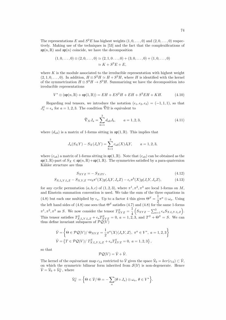
74

The representations E and S2E has highest weights (1, 0, . . . , 0) and (2, 0, . . . , 0) respec-tively. Making use of the techniques in [53] and the fact that the complexifications ofsp(n,R) and sp(n) coincide, we have the decomposition

(1, 0, . . . , 0)⊗ (2, 0, . . . , 0) ' (2, 1, 0 . . . , 0) + (3, 0, . . . , 0) + (1, 0, . . . , 0)

' K + S3E + E,

where K is the module associated to the irreducible representation with highest weight(2, 1, 0, . . . , 0). In addition, H ⊗S2H ' H +S3H, where H is identified with the kernelof the symmetrization H ⊗S2H → S3H. Summarizing we have the decomposition intoirreducible representations

V ∗ ⊗ (sp(n,R) + sp(1,R)) = EH + ES2H + EH + S3EH +KH. (4.10)

Regarding real tensors, we introduce the notation (ε1, ε2, ε3) = (−1, 1, 1), so that

J2a = εa for a = 1, 2, 3. The condition ∇Ω is equivalent to

∇XJa =

3∑b=1

dabJb, a = 1, 2, 3, (4.11)

where (dab) is a matrix of 1-forms sitting in sp(1,R). This implies that

Ja(SXY )− SX(JaY ) =

3∑b=1

cab(X)JbY, a = 1, 2, 3,

where (cab) a matrix of 1-forms sitting in sp(1,R). Note that (cab) can be obtained as thesp(1,R)-part of SX ∈ sp(n,R)+sp(1,R). The symmetries satisfied by a para-quaternionKahler structure are thus

SXY Z =− SXZY , (4.12)

SXJaY JaZ − SX,Y,Z =εbπc(X)g(JbY, JaZ)− εcπb(X)g(JcY, JaZ), (4.13)

for any cyclic permutation (a, b, c) of (1, 2, 3), where π1, π2, π3 are local 1-forms on M ,and Einstein summation convention is used. We take the sum of the three equations in

(4.8) but each one multiplied by εa. Up to a factor 4 this gives ΘS =1

2πa ⊗ ωa. Using

the left hand sides of (4.8) one sees that ΘS satisfies (4.7) and (4.8) for the same 1-forms

π1, π2, π3 as S. We now consider the tensor TSXY Z =1

4

(SXY Z −

∑3a=1 εaSXJaY JaZ

).

This tensor satisfies TSXJaY JaZ + εaTSXY Z = 0, a = 1, 2, 3, and TS + ΘS = S. We can

thus define invariant subspaces of PQ(V )

V =

Θ ∈ PQ(V )/ ΘXY Z =

1

2πa(X)〈JaY, Z〉, πa ∈ V ∗, a = 1, 2, 3

V =

T ∈ PQ(V )/ TSXJaY JaZ + εaT

SXY Z = 0, a = 1, 2, 3

,

so thatPQ(V ) = V + V.

The kernel of the equivariant map c12 restricted to V gives the space V0 = ker(c12) ⊂ V,on which the symmetric bilinear form inherited from S(V) is non-degenerate. HenceV = V0 + V⊥0 , where

V⊥0 =

Θ ∈ V/Θ = −∑a

(θ Ja)⊗ ωa, θ ∈ V ∗.

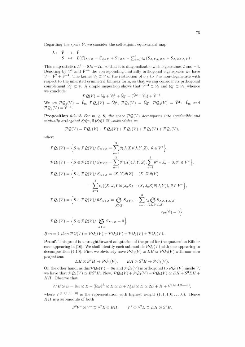
75

Regarding the space V, we consider the self-adjoint equivariant map

L : V → VS 7→ L(S)XY Z = SZXY + SY ZX −

∑3a=1 εa (SJaY JaZX + SJaZXJaY ) .

This map satisfies L2 = 8Id−2L, so that it is diagonalizable with eigenvalues 2 and −4.Denoting by V2 and V−4 the corresponding mutually orthogonal eigenspaces we haveV = V2 + V−4. The kernel V0 ⊂ V of the restriction of c12 to V is non-degenerate withrespect to the inherited symmetric bilinear form, so that we can consider its orthogonalcomplement V⊥0 ⊂ V. A simple inspection shows that V−4 ⊂ V0 and V⊥0 ⊂ V2, whencewe conclude

PQ(V ) = V0 + V⊥0 + V⊥0 + (V2 ∩ V0) + V−4.

We set PQ1(V ) = V0, PQ2(V ) = V⊥0 , PQ3(V ) = V⊥0 , PQ4(V ) = V2 ∩ V0, andPQ5(V ) = V−4.

Proposition 4.2.13 For m ≥ 8, the space PQ(V ) decomposes into irreducible andmutually orthogonal Sp(n,R)Sp(1,R)-submodules as

PQ(V ) = PQ1(V ) + PQ2(V ) + PQ3(V ) + PQ4(V ) + PQ5(V ),

where

PQ1(V ) =S ∈ PQ(V )/ SXY Z =

3∑a=1

θ(JaX)〈JaY, Z〉, θ ∈ V ∗,

PQ2(V ) =S ∈ PQ(V )/ SXY Z =

3∑a=1

θa(X)〈JaY,Z〉,3∑a=1

θa Ja = 0, θa ∈ V ∗,

PQ3(V ) =S ∈ PQ(V )/ SXY Z = 〈X,Y 〉θ(Z)− 〈X,Z〉θ(Y )

−3∑a=1

εa(〈X, JaY 〉θ(JaZ)− 〈X,JaZ〉θ(JaY )), θ ∈ V ∗,

PQ4(V ) =S ∈ PQ(V )/ 6SXY Z = S

XYZ

SXY Z −3∑a=1

εaSXJaY JaZ

SXJaY JaZ ,

c12(S) = 0,

PQ5(V ) =S ∈ PQ(V )/ S

XYZ

SXY Z = 0.

If m = 4 then PQ(V ) = PQ1(V ) + PQ2(V ) + PQ3(V ) + PQ4(V ).

Proof. This proof is a straightforward adaptation of the proof for the quaternion Kahlercase appearing in [16]. We shall identify each submodule PQi(V ) with one appearing indecomposition (4.10). First we obviously have PQ1(V ) ' EH ' PQ3(V ) with non-zeroprojections

EH ⊗ S2H → PQ1(V ), EH ⊗ S2E → PQ3(V ).

On the other hand, as dimPQ2(V ) = 8n and PQ2(V ) is orthogonal to PQ1(V ) inside V,we have that PQ2(V ) ' ES3H. Now, PQ3(V ) +PQ4(V ) +PQ5(V ) ' EH +S3EH +KH. Observe that

∧2E ⊗ E = Rω ⊗ E + (Rω)⊥ ⊗ E ' E + ∧2

0E ⊗ E ' 2E +K + V (1,1,1,0,...,0),

where V (1,1,1,0,...,0) is the representation with highest weight (1, 1, 1, 0, . . . , 0). HenceKH is a submodule of both

S2V ∗ ⊗ V ∗ ⊃ ∧2E ⊗ EH, V ∗ ⊗ ∧2E ⊃ EH ⊗ S2E.

76

Using Schur’s Lemma, an equivariant map PQ4(V ) + PQ5(V )→ ∧2E ⊗ EH will havekernel isomorphic to S3EH and will be non-zero in a submodule isomorphic to K. Themodule ∧2E ⊂ S2V ∗ can be seen as the space of bilinear forms satisfying b(Ja·, Ja·) =εab(·, ·), a = 1, 2, 3, so that we consider

p : S2V ∗ ⊗ V ∗ → ∧2E ⊗ EHT 7→ 1

4 (TXY Z −∑a εaTJaXJaY Z) .

The projection π : V ∗ ⊗ ∧2V ∗ → PQ5(V ) is given by T 7→ 16 (2− L)U where

UXY Z =1

4

(TXY Z −

∑a

εaTXJaY JaZ

).

After a long computation one can check that the image under the composition of maps

V ∗ ⊗ ∧2V ∗π→ PQ5(V )

sym→ S2V ∗ ⊗ V ∗ p→ ∧2E ⊗ EH

of an element α⊗β∧γ, α, β, γ ∈ V ∗, is never zero if β and γ are linearly independent overthe para-quaternions H (which is possible as n ≥ 2). This implies that PQ5(V ) ' KH,and therefore PQ4(V ) ' S3EH.

Making use of the isomorphisms seen in the previous proof we find

dimPQ1(V ) = dimPQ3(V ) = 4n, dimPQ2(V ) = 8n,

dimPQ4(V ) =4

3n(n+ 1)(2n+ 1), dimPQ5(V ) =

16

3n(n2 − 1).

Therefore, para-quaternion Kahler structures in the composed class PQ1 +PQ2 +PQ3

are sections of a vector bundle whose rank grows linearly with the dimension of themanifold. This motivates the following definition.

Definition 4.2.14 A homogeneous para-quaternion Kahler structure is called of lineartype if it belongs to the class PQ1 + PQ2 + PQ3.

It is easy to see that a homogeneous para-quaternion Kahler structure of linear typetakes the form

SXY = g(X,Y )ξ − g(Y, ξ)X −3∑a=1

εa (g(JaY, ξ)JaX − g(X, JaY )Jaξ)

+

3∑a=1

g(X, ζa)JaY, (4.14)

for some vector fields ξ and ζa, a = 1, 2, 3. Since the underlying metric g is not definitewe need the following further definition.

Definition 4.2.15 A homogeneous para-quaternion Kahler structure of linear type de-fined by the vector fields ξ and ζa, a = 1, 2, 3, is called

1. non-degenerate if g(ξ, ξ) = 0,

2. degenerate if g(ξ, ξ) = 0.

A homogeneous para-hyper-Kahler structure is a homogeneous structure S on a para-hyper-Kahler manifold (M, g, J1, J2, J3) satisfying ∇Ja = 0, a = 1, 2, 3. This implies

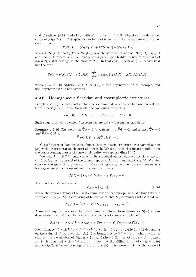
77

that S satisfies (4.12) and (4.13) with πa = 0 for a = 1, 2, 3. Therefore, the decompo-sition of PHK(V ) = V ∗ ⊗ sp(n,R) can be read in terms of the para-quaternion Kahlercase. In fact,

PHK(V ) = PHK1(V ) + PHK2(V ) + PHK3(V ),

where PHK1(V ), PHK2(V ), PHK3(V ) have the same expression as PQ3(V ), PQ4(V )and PQ5(V ) respectively. A homogeneous para-hyper-Kahler structure S is said oflinear type if it belongs to the class PHK1. In that case, S seen as (1, 2)-tensor fieldhas the form

SXY = g(X,Y )ξ − g(Y, ξ)X −3∑a=1

εa (g(JaY, ξ)JaX − g(X, JaY )Jaξ) ,

where ξ = θ]. In addition, S ∈ PHK1(V ) is said degenerate if ξ is isotropic, andnon-degenerate if ξ is non-isotropic.

4.2.6 Homogeneous Sasakian and cosymplectic structures

Let (M, g, φ, ξ, η) be an almost contact metric manifold, we consider homogeneous struc-tures S satisfying Ambrose-Singer-Kiricenko equations, that is

∇g = 0, ∇R = 0, ∇S = 0, ∇φ = 0.

Such structures will be called homogeneous almost contact metric structures.

Remark 4.2.16 The condition ∇φ = 0 is equivalent to ∇Φ = 0, and implies ∇η = 0and ∇ξ = 0 since

∇XΦ(ξ, Y ) + Φ(∇Xξ, Y ) = 0

Classification of homogeneous almost contact metric structures was carried out in[26] with a representation theoretical approach. We recall that classification and obtainthe corresponding classes of tensors. Hereafter we suppose dimM ≥ 5.

We take V = R2n+1 endowed with its standard almost contact metric structure(〈 , 〉, φ, ξ, η) as the model of the tangent space TxM at a fixed point x ∈ M . We alsoconsider the space of (0, 3)-tensors on V satisfying the same algebraic symmetries as ahomogeneous almost constant metric structure, that is,

S(V ) = S ∈ ⊗3V/SXY Z + SXZY = 0.

The condition ∇φ = 0 reads∇Xφ = [SX , φ], (4.15)

where the bracket denotes the usual commutator of endomorphisms. We thus take thesubspace S+(V ) ⊂ S(V ) consisting of tensors such that SX commutes with φ, that is

S+(V ) = S ∈ S(V )/ SXφY φZ − SXY Z = 0.

A simple computation shows that the symmetric bilinear form defined on S(V ) is non-degenerate on S+(V ), so that we can consider its orthogonal complement

S−(V ) = S ∈ S(V )/ SXφY φZ + SXY Z = η(Y )SXξZ + η(Z)SXY ξ.

Identifying S(V ) with V ∗ ⊗ (∧2V ∗) ' V ∗ ⊗ so(2p+ 1, 2q) (or so(2p, 2q + 1) dependingon the value of ε) we have that S+(V ) is isomorphic to V ∗ ⊗ u(p, q), where u(p, q) isseen as the Lie algebra of U(p, q) × 1 ⊂ O(2p + 1, 2q) (or O(2p, 2q + 1)). HenceS−(V ) is identified with V ∗ ⊗ u(p, q)⊥ (note that the Killing forms of so(2p + 1, 2q)and so(2p, 2q + 1) are non-degenerate on u(p, q)). Therefore S+(V ) is the space of

78

tensors with the same symmetries as homogeneous almost contact metric structures ona cosymplectic manifold, and S−(V ) is the space of tensors with the same symmetriesas ∇φ. In addition, due to (4.15) we have that ∇φ gives the component of S in S−(V ).It is obvious that S+(V ) is invariant under the induced U(p, q)× 1 representation onS(V ), hence so is S−(V ).

Following [26], and using the same notation as in Subsection 4.2.2, we have for n ≥ 3the decompositions into irreducible U(p, q)× 1-modules

S+(V ) = R+ 2JΛ1,0K + [Λ1,10 ] + JΛ2,1

0 K + JBK,

S−(V ) = 2R+ 2JΛ1,0K + 2[Λ1,10 ] + 2JΛ2,0K + JΛ2,1

0 K + JΛ3,0K + Jσ2,0K + JAK.

For n = 2 these decompositions are valid except that the modules JΛ2,10 K and JΛ3,0K are

absent in S−(V ), and JΛ2,10 K is absent in S+(V ). As we indicated in Section 1.2.3, a

decomposition of S−(V ) using real tensors is obtained in [22]. The irreducible submodulecorresponding to α-Sasakian structures is the one dimensional space

C6(V ) = S ∈ S−(V )/ SXY Z = αε(η(Z)〈X,Y 〉 − η(Y )〈X,Z〉), α ∈ R.

Therefore for homogeneous almost contact metric structure S on a Sasakian manifold(i.e., a 1-Sasakian manifold) the component in S−(V ) is given by

(S−)XY Z = ε(η(Z)〈X,Y 〉 − η(Y )〈X,Z〉).

We finally obtain a decomposition of S+(V ) into irreducible U(p, q)×1-modules usingreal tensors.

Proposition 4.2.17 For n ≥ 3, the space S+(V ) decomposes into irreducible and mu-tually orthogonal U(p, q)× 1-modules as

S+(V ) = CS1(V ) + CS2(V ) + CS3(V ) + CS4(V ) + CS5(V ) + CS6(V ),

where

CS1(V ) =S ∈ D2 / SXY Z =

1

2

(SZXY + SY ZX + SφZXφY + SφY φZX

),

c12(S) = 0,

CS2(V ) =S ∈ D2 / SXY Z = 〈X,Y 〉ψ1(Z)− 〈X,Z〉ψ1(Y ) + 〈X,φY 〉ψ1(φZ)

− 〈X,φZ〉ψ1(φY )− 2〈φY,Z〉ψ1(φX), ψ1 ∈ V ∗,

CS3(V ) =S ∈ D2 / SXY Z = −1

2

(SZXY + SY ZX + SφZXφY + SφY φZX

),

c12(S) = 0,

CS4(V ) =S ∈ D2 / SXY Z = 〈X,Y 〉ψ2(Z)− 〈X,Z〉ψ2(Y ) + 〈X,φY 〉ψ2(φZ)

− 〈X,φZ〉ψ2(φY ) + 2〈φY,Z〉ψ2(φX), ψ2 ∈ V ∗,

CS5(V ) =S ∈ S+(V ) / SXY Z = η(X)ω0(Y,Z)

,

CS6(V ) =S ∈ S+(V ) / trace(Sξ) = 0

.

If n=2 then S+(V ) = CS2(V ) + CS3(V ) + CS4(V ) + CS5(V ) + CS6(V ).

Proof. We first decompose V ∗ = Rη + V ∗, where V is the orthogonal complement toξ. This gives the following orthogonal decomposition into U(p, q)-modules

V ∗ ⊗ u(p, q) = (Rη + V ∗)⊗ u(p, q) = Rη ⊗ u(p, q) + V ∗ ⊗ u(p, q).

79

The first summand is isomorphic to u(p, q) and is identified with

D1 = S ∈ S+(V )/ SXY Z = η(X)SξY Z.

We can thus further decompose u(p, q) = Rω0 +su(p, q) where ω0 is the symplectic formon V inherited from Φ. This translates into D1 = CS5 ⊕ CS6. The second summandconsists of basic tensors and is identified with

D2S ∈ S+(V )/ SξY Z = 0.

Note that D2 ' V ∗⊗u(p, q) can be seen as the space of tensors with the same symmetriesas homogeneous pseudo-Kahler structures on V , so that following subsection 4.2.2 wecan decompose D2 = CS1 + CS2 + CS3 + CS4.

It is easy to see that we have isomorphisms

CS1(V ) ' JΛ2,10 K, CS2(V ) ' CS4(V ) ' JΛ1,0K, CS3(V ) ' JBK,

CS5(V ) ' R, CS6(V ) ' [Λ1,10 ],

so that the previous are irreducible U(p, q)× 1-modules.Let (M, g, φ, ξ, η) be a cosymplectic manifold, and let S be a homogeneous almost

contact metric structure on M , which we will simply call a homogeneous cosymplecticstructure. Since ∇φ = 0, the S− part of S vanishes, so that S ∈ S+. We consider theclass CS2 + CS4 + CS5. Although this class has dimension 4n+ 1 which does not growlinearly with the dimension of the manifold, it depends on two basic 1-forms and a onedimensional vertical term corresponding to the CS5 part. Therefore, in analogy withthe pseudo-Kahler case, we call S a homogeneous cosymplectic structure of linear type.The corresponding (1, 2)-vector field takes the form

SXY = g(X,Y )χ− g(χ, Y )X − g(X,φY )φχ+ g(χ, JφY )φX

− 2g(ζ, φX)φY − αη(X)φY, (4.16)

for some vector fields χ and ζ, and α ∈ R.On the other hand, let (M, g, φ, ξ, η) be a Sasakian manifold, and let S be a homoge-

neous almost contact metric structure on M , which we will simply call a homogeneousSasakian structure. Since ∇Xφ = [SX , φ] the S− part of S belongs to C6 with α = 1.We consider a homogeneous Sasakian structure whose S+ part belongs to the classCS2 + CS4 + CS5. For the same reason as before we will call S a homogeneous Sasakianstructure of linear type. The corresponding (1, 2)-tensor field takes the form

SXY = g(X,Y )χ− g(χ, Y )X − g(X,φY )φχ+ g(χ, JφY )φX

− 2g(ζ, φX)φY − αη(X)φY + g(X,Y )ξ − εη(Y )X, (4.17)

for some vector fields χ and ζ, and α ∈ R.Since the metric g restricted to the contact distribution D = Spanξ⊥ may have

signature, we have to distinguish between the following cases.

Definition 4.2.18 A homogeneous cosymplectic (Sasakian) structure of linear type iscalled

1. non-degenerate if g(χ, χ) 6= 0, and

2. degenerate if g(χ, χ) = 0.

Remark 4.2.19 The same study can be done replacing the Sasakian condition by theα-Sasakian condition, which implies that the intrinsic torsion belongs to the class C6with α not necessarily equal to 1.

Chapter 5

Homogeneous ε-Kahlerstructures of linear type

In this chapter we study homogeneous structures of linear type on pseudo-Kahler andpara-Kahler manifolds. On the one hand, we obtain that non-degenerate homogeneouspseudo-Kahler and para-Kahler structures of linear type characterize spaces of constantholomorphic and para-holomorphic sectional curvature. Moreover, if the metric is notdefinite, we show that the corresponding complex and para-complex space forms locallyadmit this kind of structures, but unlike in the Riemannian setting, the global existenceis faced with the completeness of the metric. On the other hand, we completely de-termine the holonomy and the local form of pseudo-Kahler and para-Kahler admittingdegenerate homogeneous structures of linear type. In addition we exhibit the relationbetween their underlying geometry and the geometry of homogeneous plane waves.

Since many features in the geometry of pseudo-Kahler and para-Kahler manifoldsare very similar, it is very convenient to develop the arguments and the results simul-taneously. For this reason we unify this geometries through the notion of ε-Kahlermanifolds.

Definition 5.0.20 Let (M, g) be a pseudo-Riemannian manifold.

1. An almost ε-Hermitian structure on (M, g) is a smooth section J of so(TM) suchthat J2 = εId.

2. (M, g) is called ε-Kahler if it admits a parallel almost ε-Hermitian structure J withrespect to the Levi-Civita connection.

This way, one recovers the corresponding formula or result in the pseudo-Kahler andthe para-Kahler cases by substituting ε = −1 and ε = 1 respectively. In particular wecan write a homogeneous ε-Kahler structure of linear type as

SXY = g(X,Y )ξ − g(ξ, Y )X + εg(X, JY )Jξ − εg(ξ, JY )JX − 2g(ζ, JX)JY, (5.1)

for some vector fields ξ and ζ. The notions of degenerate and non-degenerate structuresremain the same (Definitions 4.2.9 and 4.2.6). We shall also use the terms ε-complexand ε-holomorphic which include the complex and para-complex cases in the obviousway. In addition Cε will denote the complex and the para-complex numbers for ε = ±1respectively, where iε will stand for the corresponding imaginary unit.

5.1 The non-degenerate case

Lemma 5.1.1 Let (M, g, J) be a connected ε-Kahler manifold of dimension 2n > 4 ad-mitting a non-degenerate homogeneous ε-Kahler structure of linear type. Then (M, g, J)is Einstein.

81

82

Proof. The following proof has been adapted to the pseudo-Riemannian setting fromone appearing in [29] in the Riemannian case. Equation ∇R = 0 reads

(∇XR)Y ZWU = −RSXY ZWU −RY SXZWU −RY ZSXWU −RY ZWSXU , (5.2)

so applying the second Bianchi identity and substituting (5.1) we have

0 = SXYZ

2g(X, ξ)RY ZWU + g(X,W )RY ZξU + g(X,U)RY ZWξ

+ 2εg(X, JY )RJξZWU + εg(X, JW )RY ZJξU + εg(X, JU)RY ZWJξ

.

Since g(ξ, ξ) 6= 0 we can choose an orthonormal basis including ξ/√|g(ξ, ξ)|. Contracting

the previous formula with respect to X and W and applying first Bianchi identity weobtain

(2n+ 2)RZY ξU = −2g(Y, ξ)Ric(Z,U) + 2g(Z, ξ)Ric(Y,U)

− 2εg(Y, JZ)Ric(Jξ, U)− g(Y,U)Ric(Z, ξ)

− εg(Y, JU)Ric(Z, Jξ) + g(Z,U)Ric(Y, ξ)

+ εg(Z, JU)Ric(Y, Jξ),

(5.3)

where Ric is the Ricci curvature. Denoting the scalar curvature by s, we can deduceRic(Z, ξ) = (s/2n)g(Z, ξ) by contracting (5.3) with respect to Y and U with the sameorthonormal basis as before. Setting a = 1/(2n+ 2) and ν = s/2n, we can write

1

aRξU = 2θ ∧Ric(U)− 2νεθ(JU)ω + bU [ ∧ θ + ν(JU)[ ∧ (θ J), (5.4)

where ω is the symplectic form associated to g and J . Using the identity RWUJξ· =RξJWU · −RξJUW · we can write (5.3) as

0 = 2θ ∧RWU +W [ ∧RξU − U [ ∧RξW− 2εω ∧ (RξJUW −RξJWU )

− ε(JW )[ ∧RξJU + ε(JU)[ ∧RξJW .(5.5)

Denoting the right hand side of (5.4) by Ξ(U) and substituting in (5.5) we obtain

0 =2

aθ ∧RWU +W [ ∧ Ξ(U)− U [ ∧ Ξ(W )

− 2εω ∧ (iWΞ(JU)− iUΞ(JW ))

− ε(JW )[ ∧ Ξ(JU) + ε(JU)[ ∧ Ξ(JW ).

Taking W = ξ the previous formula transforms into

0 = ε(2g(ξ, ξ)ω + θ ∧ (θ J)) ∧ (Ric(JU)− ν(JU)[),

and contracting first with ξ and then with Jξ we obtain

g(ξ, ξ)(Ric(JU)− ν(JU)[) = 0.

Since g(ξ, ξ) 6= 0 we deduce that the manifold is Einstein.

Theorem 5.1.2 Let (M, g, J) be a connected ε-Kahler manifold of dimension 2n > 4admitting a non-degenerate homogeneous ε-Kahler structure S of linear type. Then(M, g, J) has constant ε-holomorphic sectional curvature c = −4g(ξ, ξ) and ζ = 0.

83

Proof. Since by the previous Lemma (M, g, J) is Einstein, formula (5.3) transformsinto

RY ZξW = cR0Y ZξW ,

where c = s/(4n(n + 1)) and R0 is the curvature of a manifold with constant ε-holomorphic sectional curvature equal to 4, i.e.,

R0XY ZW = g(Y,Z)g(X,W )− g(X,Z)g(Y,W ) + εg(X, JZ)g(Y, JW )

− εg(x, JW )g(Y, JZ) + 2εg(X,JY )g(Z, JW ).

This implies that

RXJXξ = c −2g(JX, ξ)X + 2g(X, ξ)JX − 2g(X,X)Jξ . (5.6)

On the other hand, ∇ξ = 0 is equivalent to ∇Xξ = SXξ. Using this in

RXJXξ = ∇[X,JX]ξ −∇X∇JXξ +∇JX∇Xξ,

we getRXJXξ = −g(ξ, ξ)R0

XJXξ + ΘζXJXξ, (5.7)

where

ΘζXY ξ = 2g(X, Jζ) g(Y, Jξ)ξ + g(ξ, ξ)JY + 2εg(ζ, Y )Jξ

− 2g(Y, Jζ) g(X, Jξ)ξ + g(ξ, ξ)JX + 2εg(X, ζ)Jξ+ 2 g(Y, ζ)g(ξ, JX)− g(X, ζ)g(ξ, JY ) + 2g(X, JY )g(ξ, ζ) Jξ.

Taking Y = X and X ∈ Spanζ, Jζ⊥, and comparing formulas (5.6) and (5.7), we

have that c = −g(ξ, ξ) and g(ξ, ζ) = 0. In addition, this implies that ΘζXJXξ = 0,

whence 2εg(ξ, ξ)g(X, ζ) = 0. This together with g(ξ, ζ) = 0 gives ζ = 0. Let nowA = R+ g(ξ, ξ)R0. A direct computation from (5.2) gives

(∇XR)Y ZWU = g(Y, ξ)AXZWU + g(Z, ξ)AY XWU + g(W, ξ)AY ZXU

+ g(U, ξ)AY ZWX − g(JY, ξ)AJXZWU − g(JZ, ξ)AY JXWU

− g(JW, ξ)AY ZJXU − g(JU, ξ)AY ZWJX .

Since A satisfies first Bianchi identity, taking cyclic sum in X,Y, Z we obtain

0 = −2 SXYZ

g(X, ξ)AY ZWU ,

which is equivalent to θ ∧ AWU = 0. Contracting with ξ and taking into account thatAY ZξW = 0 we have that

0 = g(ξ, ξ)AWU ,

hence AWU = 0. This proves that (M, g, J) has constant ε-holomorphic sectional cur-vature −4g(ξ, ξ).

Remark 5.1.3 For ε = −1, if g(ξ, ξ) > 0 then c = −4g(ξ, ξ) < 0, so that spaces withnegative definite metric and constant negative holomorphic sectional curvature cannotadmit non-degenerate homogeneous pseudo-Kahler structures of linear type. Similarly, ifg(ξ, ξ) < 0 then c > 0, so that spaces with positive definite metric and constant positiveholomorphic sectional curvature are also excluded.

84

5.2 The degenerate case

Equation ∇R = 0 reads

(∇XR)Y ZWU = −RSXY ZWU −RY SXZWU −RY ZSXWU −RY ZWSXU , (5.8)

so applying second Bianchi identity and substituting (5.1) we have

0 = SXYZ

2g(X, ξ)RY ZWU + g(X,W )RY ZξU + g(X,U)RY ZWξ

+2εg(X, JY )RJξZWU + εg(X, JW )RY ZJξU + εg(X, JU)RY ZWJξ . (5.9)

Since g(ξ, ξ) = 0, there exists an orthonormal basis ek such that g(e1, e1) = 1,g(e2, e2) = −1, and ξ = g(ξ, e1)(e1 + e2). Whence, contracting the previous formulawith respect to X and W and applying first Bianchi identity, we obtain

(2n+ 2)RZY ξU = −2g(Y, ξ)Ric(Z,U) + 2g(Z, ξ)Ric(Y,U)

−2εg(Y, JZ)Ric(Jξ, U)− g(Y, U)Ric(Z, ξ) (5.10)

−εg(Y, JU)Ric(Z, Jξ) + g(Z,U)Ric(Y, ξ)

+εg(Z, JU)Ric(Y, Jξ).

With the same orthonormal basis, contracting the previous expression with respect toY and U we arrive to Ric(Z, ξ) = (s/2n)g(Z, ξ). Setting a = 1/(2n+ 2) and ν = s/2n,we can write

1

aRξU = 2θ ∧Ric(U)− 2νεθ(JU)ω + νU [ ∧ θ − εν(JU)[ ∧ (θ J), (5.11)

where ω denotes the symplectic form associated to (g, J). From first Bianchi identitywe have RWUJξ· = RξJWU · −RξJUW · so we can write (5.10) as

0 = 2θ ∧RWU +W [ ∧RξU − U [ ∧RξW−2εω ∧ (RξJUW −RξJWU ) (5.12)

−ε(JW )[ ∧RξJU + ε(JU)[ ∧RξJW .

Denoting by Ξ(U) the right hand side of (5.11) and substituting in (5.12) we obtain

0 =2

aθ ∧RWU +W [ ∧ Ξ(U)− U [ ∧ Ξ(W )

−2εω ∧ (iWΞ(JU)− iUΞ(JW ))

−ε(JW )[ ∧ Ξ(JU) + ε(JU)[ ∧ Ξ(JW ).

Then, taking W = ξ in the previous formula

0 = ε(θ ∧ (θ J)) ∧ (Ric(JU)− ν(JU)[).

Now, since U is arbitrary, denoting α = Ric− νg, one has

θ ∧ (θ J) ∧ α(X) = 0,

for any vector field X. This implies that

α = λθ + µθ J,

for some 1-forms λ and µ. Note that since (M, g, J) is ε-Kahler, α = Ric − νg issymmetric and of type (1, 1). Imposing this to the right hand side of the previousequation we have that

λ = fθ, µ = −εf(θ J),

85

for some function f , so that we obtain

Ric = νg + f (θ ⊗ θ − ε(θ J)⊗ (θ J)) . (5.13)

Substituting (5.13) in (5.11)

1

aRξU = νR0

ξU + PξU , (5.14)

where again

R0XY ZW = g(Y,Z)g(X,W )− g(X,Z)g(Y,W ) + εg(X, JZ)g(Y, JW )

− εg(x, JW )g(Y, JZ) + 2εg(X,JY )g(Z, JW ).

andPξU = −2εfθ(JU)θ ∧ (θ J).

On the other hand, from ∇ξ = S · ξ and (5.1), formula

RXY Z = ∇[X,Y ]Z − [∇X ,∇Y ]Z

givesRXY ξ = −g(ξ, ξ)R0

XY ξ + ΘζXY ξ = Θζ

XY ξ, (5.15)

where

ΘζXY ξ =− 2g(ζ, JY )g(X,Jξ)ξ + 2g(ζ, Y )g(X, Jξ)Jξ − 4g(ζ, JY )g(X, ξ)Jξ

+ 2g(ζ, JX)g(Y, Jξ)ξ − 2g(ζ,X)g(Y, Jξ)Jξ + 4g(ζ, JX)g(Y, ξ)Jξ

+ 4g(ξ, ζ)g(Y, JX)Jξ − 4εg(ζ, JY )g(ξ,X)Jξ + 4εg(ζ, JX)g(ζ, Y )Jξ.

Taking Y = JX and comparing (5.14) and (5.15) one finds that

2abg(ξ, JX) = 0, 2abg(ξ,X) = 0,

for every X, so that ν = 0. Hence the scalar curvature vanishes. We now choose a basis

ξ, Jξ, q1, Jq1, Xi, JXi

of TpM for every p ∈ M , where g(ξ, q1) = 1, g(q1, q1) 6= 0, and Xi, JXi is an or-thonormal basis of Spanξ, Jξ, q1, Jq1⊥. Comparing again (5.14) and (5.15) for X = ξand Y = Jq1, and for X = Jξ and Y = Jq1 we obtain that g(ζ, Jξ) = 0 and g(ζ, ξ) = 0,so that ζ ∈ Spanξ, Jξ⊥. Taking X = Xi and Y = Jq1, and X = JXi and Y = Jq1 wealso have g(ζ, JXi) = 0 and g(ζ,Xi) = 0 respectively, so that ζ ∈ Spanξ, Jξ. Finally,writing ζ = λξ + µJξ for some functions λ and µ, and taking X = q1 and Y = Jq1 onefinds g(ζ, Jq1) = 0 and 2af = −2ελ− 4λ2, so that

ζ = λξ, f = −1

aλ(ε+ 2λ).

Note that equations ∇ξ = 0 and ∇ζ = 0 imply that λ must be constant. This agreeswith the fact that the Ricci form

ρ = fθ ∧ (θ J)

is closed as (M, g, J) is ε-Kahler. We have proved

Proposition 5.2.1 Let (M, g, J) be an ε-Kahler manifold admitting a degenerate ε-Kahler homogeneous structure of linear type given by (5.1). Then ζ = λξ for someλ ∈ R and the Ricci curvature is

Ric = −1

aλ(ε+ 2λ) (θ ⊗ θ − ε(θ J)⊗ (θ J)) ,

where a = 1/(dimM + 2) and θ = ξ[. In particular the scalar curvature vanishes.

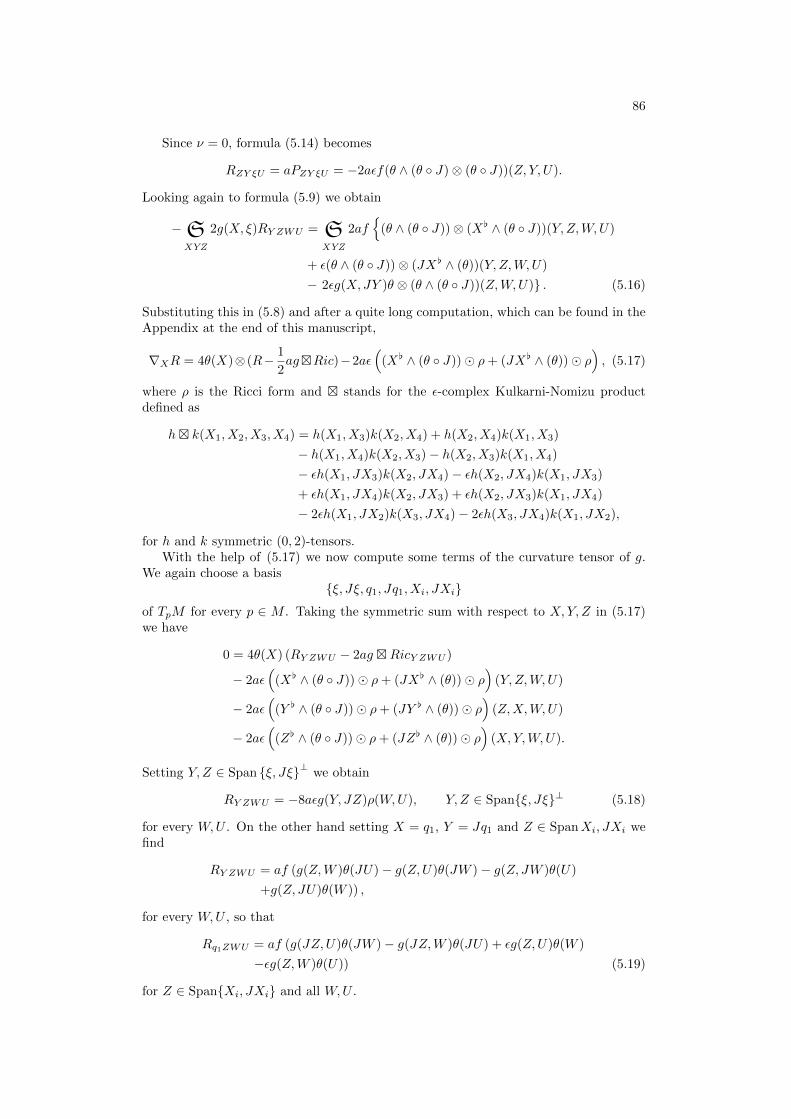
86

Since ν = 0, formula (5.14) becomes

RZY ξU = aPZY ξU = −2aεf(θ ∧ (θ J)⊗ (θ J))(Z, Y, U).

Looking again to formula (5.9) we obtain

−SXYZ

2g(X, ξ)RY ZWU = SXYZ

2af

(θ ∧ (θ J))⊗ (X[ ∧ (θ J))(Y,Z,W,U)

+ ε(θ ∧ (θ J))⊗ (JX[ ∧ (θ))(Y,Z,W,U)

− 2εg(X,JY )θ ⊗ (θ ∧ (θ J))(Z,W,U) . (5.16)

Substituting this in (5.8) and after a quite long computation, which can be found in theAppendix at the end of this manuscript,

∇XR = 4θ(X)⊗ (R− 1

2agRic)−2aε

((X[ ∧ (θ J)) ρ+ (JX[ ∧ (θ)) ρ

), (5.17)

where ρ is the Ricci form and stands for the ε-complex Kulkarni-Nomizu productdefined as

h k(X1, X2, X3, X4) = h(X1, X3)k(X2, X4) + h(X2, X4)k(X1, X3)

− h(X1, X4)k(X2, X3)− h(X2, X3)k(X1, X4)

− εh(X1, JX3)k(X2, JX4)− εh(X2, JX4)k(X1, JX3)

+ εh(X1, JX4)k(X2, JX3) + εh(X2, JX3)k(X1, JX4)

− 2εh(X1, JX2)k(X3, JX4)− 2εh(X3, JX4)k(X1, JX2),

for h and k symmetric (0, 2)-tensors.With the help of (5.17) we now compute some terms of the curvature tensor of g.

We again choose a basisξ, Jξ, q1, Jq1, Xi, JXi

of TpM for every p ∈ M . Taking the symmetric sum with respect to X,Y, Z in (5.17)we have

0 = 4θ(X) (RY ZWU − 2ag RicY ZWU )

− 2aε(

(X[ ∧ (θ J)) ρ+ (JX[ ∧ (θ)) ρ)

(Y,Z,W,U)

− 2aε(

(Y [ ∧ (θ J)) ρ+ (JY [ ∧ (θ)) ρ)

(Z,X,W,U)

− 2aε(

(Z[ ∧ (θ J)) ρ+ (JZ[ ∧ (θ)) ρ)

(X,Y,W,U).

Setting Y,Z ∈ Span ξ, Jξ⊥ we obtain

RY ZWU = −8aεg(Y, JZ)ρ(W,U), Y, Z ∈ Spanξ, Jξ⊥ (5.18)

for every W,U . On the other hand setting X = q1, Y = Jq1 and Z ∈ SpanXi, JXi wefind

RY ZWU = af (g(Z,W )θ(JU)− g(Z,U)θ(JW )− g(Z, JW )θ(U)

+g(Z, JU)θ(W )) ,

for every W,U , so that

Rq1ZWU = af (g(JZ,U)θ(JW )− g(JZ,W )θ(JU) + εg(Z,U)θ(W )

−εg(Z,W )θ(U)) (5.19)

for Z ∈ SpanXi, JXi and all W,U .

87

Proposition 5.2.2 (M, g, J) is Ricci-flat.

Proof. Let g(q1, q1) = b and suppose for the sake of simplicity that b > 0 (the caseb < 0 is analogous). Denoting q2 = Jq1, we choose an orthonormal basis√

b(ξ − q1

b

),√b(Jξ − q2

b

),q1√b,q2√b,Xi, JXi

of TpM for every p ∈ M , which has signature (−1, ε, 1,−ε, εi,−εεi) where g(Xi, Xi) =εi ∈ ±1. We compute the Ricci curvature by contracting the curvature tensor withrespect to this orthonormal basis and using (5.18) and (5.19):

Ric(W,U) = −R(W,√b(ξ − q1

b

), U,√b(ξ − q1

b

))+ εR

(W,√b(ξ − q2

b

), U,√b(ξ − q2

b

))+R

(W,

q1√b, U,

q1√b

)− εR

(W,

q2√b, U,

q2√b

)+ εiR(W,Xi, U,Xi)− εεiR(W,JXi, U, JXi)

= 4af (θ ⊗ θ − ε(θ J)⊗ (θ J))

+ 2afε∑i

εi (θ ⊗ θ − ε(θ J)⊗ (θ J))

= (4a+ 2aε∑i

εi)Ric(W,U).

We deduce that if Ric(W,U) 6= 0 then 4a+ 2aε∑i εi = 1, therefore

dimM + 2 = 4 + 2aε∑i

εi,

whencedimM = 2 + 2aε

∑i

εi < dimM.

Since this is impossible we conclude that Ric = 0.

Corollary 5.2.3 The only possible values for λ are λ = 0 and λ = − ε2 .

In the next section we shall study the cases λ = 0 and λ = − ε2 separately.

Proposition 5.2.4 The curvature tensor of g is given by

R = k(θ ∧ (θ J))⊗ (θ ∧ (θ J)),

for some function k. Moreover, if k 6= 0 the holonomy algebra of g is given by

hol ∼= R

iε iε 0−iε −iε 00 0 0n

,

which is a one dimensional subalgebra of su(1, 1) ⊂ su(p, q), p+ q = n+ 2, for ε = −1,and sl(2,R) ⊂ sl(n+ 2,R) for ε = 1.

Proof. Since (M, g, J) is Ricci-flat (5.17) becomes

∇R = 4θ ⊗R.

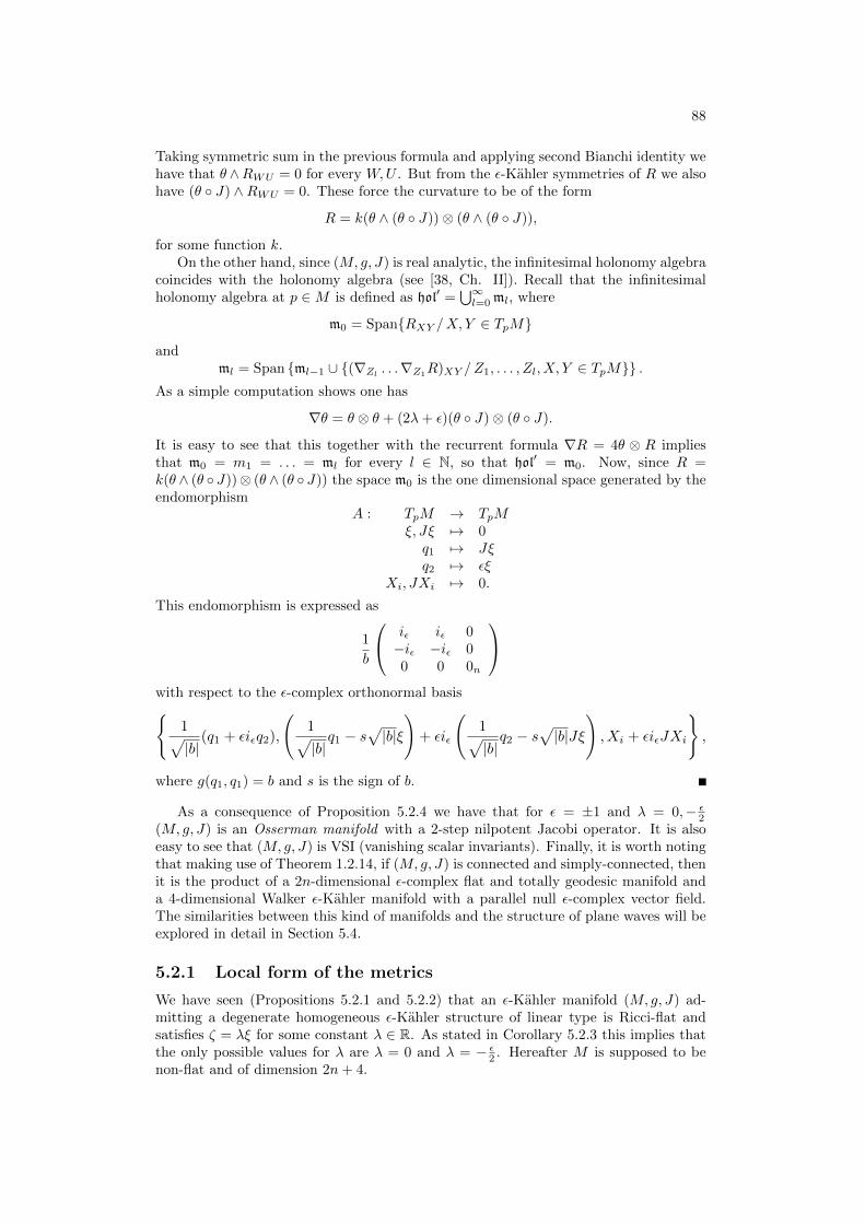
88

Taking symmetric sum in the previous formula and applying second Bianchi identity wehave that θ ∧RWU = 0 for every W,U . But from the ε-Kahler symmetries of R we alsohave (θ J) ∧RWU = 0. These force the curvature to be of the form

R = k(θ ∧ (θ J))⊗ (θ ∧ (θ J)),

for some function k.On the other hand, since (M, g, J) is real analytic, the infinitesimal holonomy algebra

coincides with the holonomy algebra (see [38, Ch. II]). Recall that the infinitesimalholonomy algebra at p ∈M is defined as hol′ =

⋃∞l=0 ml, where

m0 = SpanRXY /X, Y ∈ TpM

andml = Span ml−1 ∪ (∇Zl . . .∇Z1R)XY /Z1, . . . , Zl, X, Y ∈ TpM .

As a simple computation shows one has

∇θ = θ ⊗ θ + (2λ+ ε)(θ J)⊗ (θ J).

It is easy to see that this together with the recurrent formula ∇R = 4θ ⊗ R impliesthat m0 = m1 = . . . = ml for every l ∈ N, so that hol′ = m0. Now, since R =k(θ ∧ (θ J))⊗ (θ ∧ (θ J)) the space m0 is the one dimensional space generated by theendomorphism

A : TpM → TpMξ, Jξ 7→ 0q1 7→ Jξq2 7→ εξ

Xi, JXi 7→ 0.

This endomorphism is expressed as

1

b

iε iε 0−iε −iε 00 0 0n

with respect to the ε-complex orthonormal basis

1√|b|

(q1 + εiεq2),

(1√|b|q1 − s

√|b|ξ

)+ εiε

(1√|b|q2 − s

√|b|Jξ

), Xi + εiεJXi

,

where g(q1, q1) = b and s is the sign of b.

As a consequence of Proposition 5.2.4 we have that for ε = ±1 and λ = 0,− ε2

(M, g, J) is an Osserman manifold with a 2-step nilpotent Jacobi operator. It is alsoeasy to see that (M, g, J) is VSI (vanishing scalar invariants). Finally, it is worth notingthat making use of Theorem 1.2.14, if (M, g, J) is connected and simply-connected, thenit is the product of a 2n-dimensional ε-complex flat and totally geodesic manifold anda 4-dimensional Walker ε-Kahler manifold with a parallel null ε-complex vector field.The similarities between this kind of manifolds and the structure of plane waves will beexplored in detail in Section 5.4.

5.2.1 Local form of the metrics

We have seen (Propositions 5.2.1 and 5.2.2) that an ε-Kahler manifold (M, g, J) ad-mitting a degenerate homogeneous ε-Kahler structure of linear type is Ricci-flat andsatisfies ζ = λξ for some constant λ ∈ R. As stated in Corollary 5.2.3 this implies thatthe only possible values for λ are λ = 0 and λ = − ε

2 . Hereafter M is supposed to benon-flat and of dimension 2n+ 4.

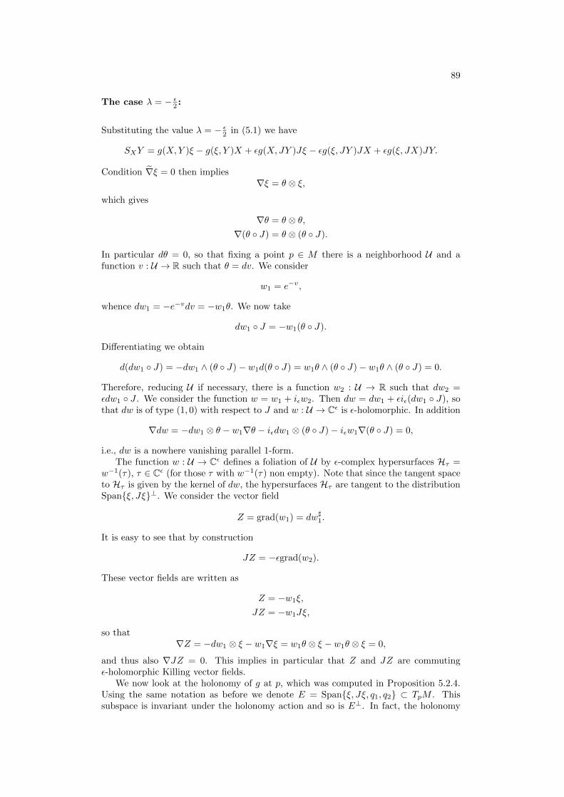
89

The case λ = − ε2 :

Substituting the value λ = − ε2 in (5.1) we have

SXY = g(X,Y )ξ − g(ξ, Y )X + εg(X,JY )Jξ − εg(ξ, JY )JX + εg(ξ, JX)JY.

Condition ∇ξ = 0 then implies∇ξ = θ ⊗ ξ,

which gives

∇θ = θ ⊗ θ,∇(θ J) = θ ⊗ (θ J).

In particular dθ = 0, so that fixing a point p ∈ M there is a neighborhood U and afunction v : U → R such that θ = dv. We consider

w1 = e−v,

whence dw1 = −e−vdv = −w1θ. We now take

dw1 J = −w1(θ J).

Differentiating we obtain

d(dw1 J) = −dw1 ∧ (θ J)− w1d(θ J) = w1θ ∧ (θ J)− w1θ ∧ (θ J) = 0.

Therefore, reducing U if necessary, there is a function w2 : U → R such that dw2 =εdw1 J . We consider the function w = w1 + iεw2. Then dw = dw1 + εiε(dw1 J), sothat dw is of type (1, 0) with respect to J and w : U → Cε is ε-holomorphic. In addition

∇dw = −dw1 ⊗ θ − w1∇θ − iεdw1 ⊗ (θ J)− iεw1∇(θ J) = 0,

i.e., dw is a nowhere vanishing parallel 1-form.The function w : U → Cε defines a foliation of U by ε-complex hypersurfaces Hτ =

w−1(τ), τ ∈ Cε (for those τ with w−1(τ) non empty). Note that since the tangent spaceto Hτ is given by the kernel of dw, the hypersurfaces Hτ are tangent to the distributionSpanξ, Jξ⊥. We consider the vector field

Z = grad(w1) = dw]1.

It is easy to see that by construction

JZ = −εgrad(w2).

These vector fields are written as

Z = −w1ξ,

JZ = −w1Jξ,

so that∇Z = −dw1 ⊗ ξ − w1∇ξ = w1θ ⊗ ξ − w1θ ⊗ ξ = 0,

and thus also ∇JZ = 0. This implies in particular that Z and JZ are commutingε-holomorphic Killing vector fields.

We now look at the holonomy of g at p, which was computed in Proposition 5.2.4.Using the same notation as before we denote E = Spanξ, Jξ, q1, q2 ⊂ TpM . Thissubspace is invariant under the holonomy action and so is E⊥. In fact, the holonomy

90

action on E⊥ is trivial. This implies that, using the parallel transport with respectto ∇, we can extend an orthonormal basis (Xa)|p, (JXa)|p, a = 1, . . . , n of E⊥ toan orthonormal reference Xa, JXa, a = 1, . . . , n on U such that ∇Xa = 0 = ∇JXa,a = 1, . . . , n. In particular they are commuting ε-holomorphic Killing vector fields. Inaddition, let γ be any smooth curve on U , we have

d

dt

∣∣∣∣t=0

(dw(Xa)γ(t)

)=(∇γ(t)dw

)(Xa) + dw

(∇γ(t)Xa

)= 0,

whence the functions dw(Xa) are constant along γ and take the value 0 at p. Thisimplies that Xa and thus JXa are tangent to the foliation Hτ . Finally note that sincethey are parallel, Xa and JXa commute with Z and JZ.

We have thus constructed a set of commuting para-holomorphic Killing vector fieldsZ, JZ,Xa, JXa tangent to Hτ . Therefore, reducing U if necessary, we can take ε-complex coordinates w, z, za on U such that ∂z = 1

2 (Z+εiεJZ), ∂za = 12 (Xa+εiεJXa).

Note that since the distributions Span∂w, ∂z and Span∂za , a = 1, . . . , n are invariantby holonomy, the vector fields Xa and JXa are orthogonal to Span∂w, ∂z. We writez = z1 + iεz

2, za = xa + iεya and w = w1 + iεw

2, and rearrange the coordinates asz1, z2, w1, w2, xa, ya. The metric with respect to these coordinates is

g =

0 0 1 0 0 . . . 00 0 0 −ε 0 . . . 01 0 b 0 0 . . . 00 −ε 0 −εb 0 . . . 00 0 0 0...

......

... Σ0 0 0 0

, (5.20)

for some function b, where

Σ = diag(

(εa 00 −εεa

), a = 1, . . . , n),

with εa = g(Xa, Xa) ∈ ±1. In addition, the ε-complex structure reads

J =

0 ε1 0

. . .

0 ε1 0

. (5.21)

Imposing that ∂z1 , ∂z2 , ∂xa and ∂ay are parallel, it is easy to see that b does not dependon z1, z2, xa, ya.

Finally, computing the curvature tensor with respect to those coordinates we obtain

R =1

2∆εb(dw1 ∧ dw2)⊗ (dw1 ∧ dw2),

where

∆ε = −ε ∂2

∂(w1)2+

∂2

∂(w2)2.

Denoting F = ∆εb and taking into account that dw1 and dw2 are parallel, we have that

∇R =1

2dF ⊗ (dw1 ∧ dw2)⊗ (dw1 ∧ dw2).

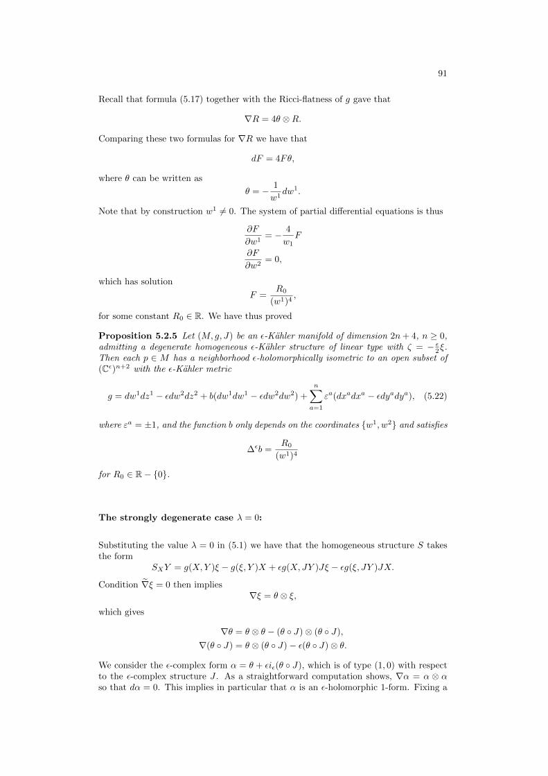
91

Recall that formula (5.17) together with the Ricci-flatness of g gave that

∇R = 4θ ⊗R.

Comparing these two formulas for ∇R we have that

dF = 4Fθ,

where θ can be written as

θ = − 1

w1dw1.

Note that by construction w1 6= 0. The system of partial differential equations is thus

∂F

∂w1= − 4

w1F

∂F

∂w2= 0,

which has solution

F =R0

(w1)4,

for some constant R0 ∈ R. We have thus proved

Proposition 5.2.5 Let (M, g, J) be an ε-Kahler manifold of dimension 2n+ 4, n ≥ 0,admitting a degenerate homogeneous ε-Kahler structure of linear type with ζ = − ε

2ξ.Then each p ∈ M has a neighborhood ε-holomorphically isometric to an open subset of(Cε)n+2 with the ε-Kahler metric

g = dw1dz1 − εdw2dz2 + b(dw1dw1 − εdw2dw2) +

n∑a=1

εa(dxadxa − εdyadya), (5.22)

where εa = ±1, and the function b only depends on the coordinates w1, w2 and satisfies

∆εb =R0

(w1)4

for R0 ∈ R− 0.

The strongly degenerate case λ = 0:

Substituting the value λ = 0 in (5.1) we have that the homogeneous structure S takesthe form

SXY = g(X,Y )ξ − g(ξ, Y )X + εg(X, JY )Jξ − εg(ξ, JY )JX.

Condition ∇ξ = 0 then implies∇ξ = θ ⊗ ξ,

which gives

∇θ = θ ⊗ θ − (θ J)⊗ (θ J),

∇(θ J) = θ ⊗ (θ J)− ε(θ J)⊗ θ.

We consider the ε-complex form α = θ + εiε(θ J), which is of type (1, 0) with respectto the ε-complex structure J . As a straightforward computation shows, ∇α = α ⊗ αso that dα = 0. This implies in particular that α is an ε-holomorphic 1-form. Fixing a

92

point p ∈M , by the closeness of α, there is a neighborhood U of p and an ε-holomorphicfunction v : U → Cε such that α = dv. We consider the ε-holomorphic function

w = e−v,

where the the exponential must read ex+iεy = ex(cos y+iε sin y) for ε = −1 and ex+iεy =ex(cosh y + iε sinh y) for ε = 1. Differentiating we obtain that

dw = −wα,

so that ∇dw = 0. This means that dw is a nowhere vanishing parallel ε-holomorphic 1-form on U . The function w : U → Cε defines a foliation of U by ε-complex hypersurfacesHτ = w−1(τ), τ ∈ Cε (for those τ with w−1(τ) non empty). Note that since the tangentspace to Hτ is given by the kernel of dw, the hypersurfaces Hτ are tangent to thedistribution Spanξ, Jξ⊥. Writing w = w1 + iεw

2, we take the vector fields

Z = (dw1)], JZ = −ε(dw2)].

These vector fields are obviously tangent to the foliation given byHτ , and since∇dw = 0we have ∇Z = 0 and ∇JZ = 0. This implies in particular that Z, JZ are commutingε-holomorphic Killing vector fields.

Making use of Proposition 5.2.4, and by the same arguments used for the case λ =−ε/2, we take coordinates w, z, za, a = 1, . . . , n, such that ∂za = 1

2 (Z + εiεJZ) and∇∂za = 0. Writing z = z1 + iεz

2, za = xa + iεya, and w = w1 + iεw

2, with respect toreal coordinates z1, z2, w1, w2, xa, ya the metric g and the complex structure J takethe form (5.20) and (5.21) respectively, where b does not depend on z1, z2, xa, ya. As astraightforward computation shows,

R =1

2∆εb(dw1 ∧ dw2)⊗ (dw1 ∧ dw2),

and

θ =−1

(w1)2 − ε(w2)2(w1dw1 − εw2dw

2).

Finally, imposing ∇R = 4θ⊗R and denoting F = ∆εb, we obtain the system of partialdifferential equations

∂F

∂w1=

−4w1

(w1)2 − ε(w2)2F

∂F

∂w2=

4εw2

(w1)2 − ε(w2)2F,

which has solution

F =R0

((w1)2 − ε(w2)2)2,

for some constant R0 ∈ R. Note that since w = e−v we always have (w1)2− ε(w2)2 6= 0.We have thus proved

Proposition 5.2.6 Let (M, g, J) be an ε-Kahler manifold of dimension 2n+ 4, n ≥ 0,admitting a strongly degenerate homogeneous ε-Kahler structure of linear type S. Theneach p ∈M has a neighborhood ε-holomorphically isometric to an open subset of (Cε)n+2

with the ε-Kahler metric

g = dw1dz1 − εdw2dz2 + b(dw1dw1 − εdw2dw2) +

n∑a=1

εa(dxadxa − εdyadya), (5.23)

where εa = ±1, and the function b only depends on the coordinates w1, w2 and satisfies

∆εb =R0

((w1)2 − ε(w2)2)2

for R0 ∈ R− 0.

93

The manifold ((Cε)n+2, g)

Propositions 5.2.6 and 5.2.5 give the local forms (5.23) and (5.22) of the metric ofa manifold with a degenerate homogeneous ε-Kahler structure of linear type. Thismotivates the study of the space (Cε)2+n endowed with this particular ε-Kahler metric,which can thus be understood as the simplest instance of this type of manifolds. Inparticular, the goal is to study the singular nature of this spaces. We shall restrictsourselves to the Lorentz ε-Kahler case, i.e., metrics of index 2. Throughout this section‖w‖λ must be understood as

‖w‖2λ =

w2

1 − εw22 for λ = 0,

w21 for λ = −ε/2. (5.24)

In addition ∆ε shall stand for the differential operator

∆ε = −ε ∂2

∂w21

+∂2

∂w22

.

We thus consider the manifold (Cε)2+n = (R2n+4, J0), where J0 is the standardε-complex structure, with real coordinates z1, z2, w1, w2, xa, ya, endowed with themetric

g = dw1dz1 − εdw2dz2 + b(dw1dw1 − εdw2dw2) +

n∑a=1

(dxadxa − εdyadya), (5.25)

where b is a function of the variables (w1, w2) satisfying

∆εb =R0

‖w‖4λ, R0 ∈ R− 0. (5.26)

As computed before, the curvature (1, 3)-tensor field of g is

R =1

2

R0

‖w‖4λ

((dw1 ∧ dw2)⊗ (dw1 ⊗ ∂z2) + ε(dw1 ∧ dw2)⊗ (dw2 ⊗ ∂z1)

).

As R0 6= 0, the curvature exhibits a singular behavior at

S = ‖w‖λ = 0.

This set can be understood as a singularity of g in the cosmological sense: the geodesicdeviation equation is governed by the components Rz

j

w1w2wi , i, j = 1, 2, of the curvaturetensor field, making the tidal forces infinite at S. Indeed, we can compute a componentof the curvature tensor with respect to an orthonormal parallel frame along a geodesicreaching the singular set in finite time, and see that it is singular (see [55]). Let γ bethe geodesic with initial value γ(0) = (0, 0, 1, 0, . . . , 0) and γ = (0, 0,−1, 0, . . . , 0). It iseasy to see that this geodesic is of the form

γ(t) = (z1(t), z2(t), 1− t, 0, xa(t), ya(t))

for some functions z1(t), z2(t), xa(t), ya(t), a = 1, . . . , n, and reaches the singular set Sat t = 1. Let

E(t) = W 1(t)∂w1 +W 2(t)∂w2 + Z1(t)∂z1 + Z2(t)∂z2 +Xa(t)∂xa + Y a(t)∂ya

be a vector field along γ. E is parallel if the following equations hold:

0 = W 1, 0 = W 2,

0 = Z1 −W 1Γz1

w1w1 −W 2Γz1

w1w2 , 0 = Z2 −W 1Γz2

w1w1 −W 2Γz2

w1w2 ,

0 = Xa, 0 = Y a.

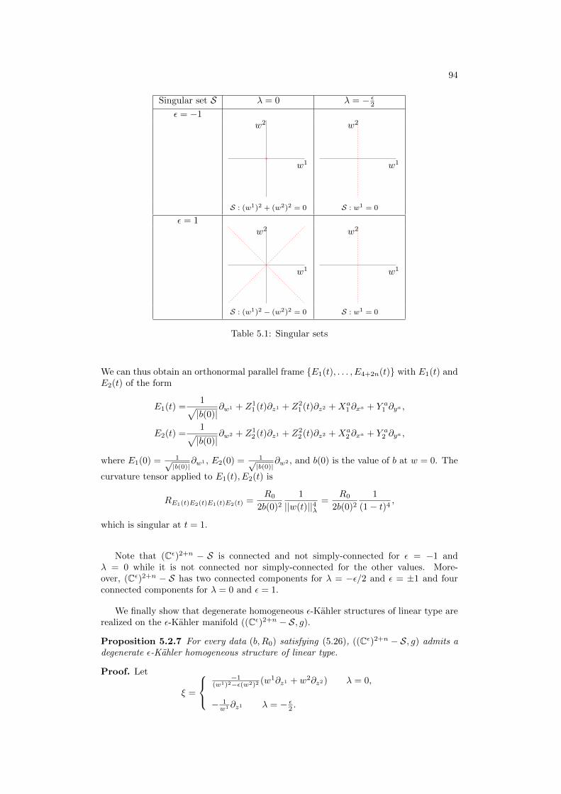
94

Singular set S λ = 0 λ = − ε2

ε = −1

w1

w2

w1

w2

S : (w1)2 + (w2)2 = 0 S : w1 = 0

ε = 1

w1

w2

w1

w2

S : (w1)2 − (w2)2 = 0 S : w1 = 0

Table 5.1: Singular sets

We can thus obtain an orthonormal parallel frame E1(t), . . . , E4+2n(t) with E1(t) andE2(t) of the form

E1(t) =1√|b(0)|

∂w1 + Z11 (t)∂z1 + Z2

1 (t)∂z2 +Xa1 ∂xa + Y a1 ∂ya ,

E2(t) =1√|b(0)|

∂w2 + Z12 (t)∂z1 + Z2

2 (t)∂z2 +Xa2 ∂xa + Y a2 ∂ya ,

where E1(0) = 1√|b(0)|

∂w1 , E2(0) = 1√|b(0)|

∂w2 , and b(0) is the value of b at w = 0. The

curvature tensor applied to E1(t), E2(t) is

RE1(t)E2(t)E1(t)E2(t) =R0

2b(0)2

1

||w(t)||4λ=

R0

2b(0)2

1

(1− t)4,

which is singular at t = 1.

Note that (Cε)2+n − S is connected and not simply-connected for ε = −1 andλ = 0 while it is not connected nor simply-connected for the other values. More-over, (Cε)2+n − S has two connected components for λ = −ε/2 and ε = ±1 and fourconnected components for λ = 0 and ε = 1.

We finally show that degenerate homogeneous ε-Kahler structures of linear type arerealized on the ε-Kahler manifold ((Cε)2+n − S, g).

Proposition 5.2.7 For every data (b, R0) satisfying (5.26), ((Cε)2+n − S, g) admits adegenerate ε-Kahler homogeneous structure of linear type.

Proof. Let

ξ =

−1

(w1)2−ε(w2)2 (w1∂z1 + w2∂z2) λ = 0,

− 1w1 ∂z1 λ = − ε

2 .

95

We take the tensor field

SXY = g(X,Y )ξ − g(ξ, Y )X + εg(X, JY )Jξ − εg(ξ, JY )JX − 2λg(ξ, JX)JY.

A straightforward computation shows that ∇ξ = 0 and ∇R = 0, where ∇ = ∇ − S,so that S is a degenerate homogeneous ε-Kahler structure of linear type (see (4.3) and(4.5)).

5.3 Infinitesimal models, homogeneous models andcompleteness

Recall the definition of infinitesimal model, transvection algebra and homogeneousmodel associated to a homogeneous structure (Section 2.3). The aim of this sectionis to prove the following results.

Theorem 5.3.1 With the exception of CPn0 and CHnn , the indefinite ε-complex space

forms CPnp , CHnp and CPn locally admit a non-degenerate homogeneous ε-Kahler struc-

ture of linear type.

Theorem 5.3.2 Let (M, g, J) be a connected and simply-connected ε-Kahler manifoldwith dimM > 4 admitting a non-degenerate homogeneous ε-Kahler structure of lineartype. If g is not definite then (M, g, J) is not complete. On the other hand, the homo-geneous model associated to a degenerate homogeneous ε-Kahler structure of linear typeis not complete.

Remark 5.3.3 Note that Theorem 5.3.2 implies that the indefinite ε-complex spaceforms CPnp , CHn

p and CPn do not admit a globally defined homogeneous ε-Kahler struc-ture of linear type except for the definite cases CPnn and CHn

0 .

We now explain the general procedure to prove Theorems 5.3.1 and 5.3.2. Thisprocedure will be then specified for each case: degenerate and non-degenerate, andpseudo-Kahler and para-Kahler. The same procedure will be used for the case of pseudo-quaternion and para-quaternion structures later in Section 6.2.

Procedure for the proof of Theorems 5.3.1 and 5.3.2.The first step is to explicitly compute the infinitesimal model and the transvection

algebra g = TpM ⊕ hol∇ associated to a homogeneous ε-Kahler structure of linear type.

This is done by obtaining the expression for R = R−RS . Denoting h = hol∇, we nextshow that the transvection algebra (g, h) is regular, that is, H is a closed subgroup ofG, where G is the simply-connected Lie group with Lie algebra g and H is its connectedLie subgroup with Lie algebra h . In order to prove that we obtain a matrix realizationof h and g in gl(N,R) for some N ∈ N, and we exponentiate it to see that the connectedLie subgroup of GL(N,R) with Lie algebra h is closed in GL(N,R), whence H must beclosed in G. For the degenerate case this is done using the adjoint representation. Forthe non-degenerate case, by Remark 1.2.18, we will only need to consider the spacesCHn

p and CPn, since by Theorem 5.1.2 our spaces of linear type are locally ±-isometric

to one of these models. Recalling the expressions (1.1) and (1.2) of CHns and CPn as

symmetric spaces Isom/Isot, we identify g with a subalgebra of isom, in such a waythat h is the intersection of g and isot. This gives a matrix realization of g and h, andsubgroups G ⊂ Isom and H ⊂ Isot, and we find that H is closed in Isom (which isclosed in Gl(m,R)). We can thus take the homogeneous model G/H associated to S.Continuing with the non-degenerate case, the orbit of p = eIsot in the model spaceIsom/Isot is just G/H. Counting dimensions one sees that G/H is an open subset of

96

Isom/Isot. Since by construction G/H admits a non-degenerate homogeneous ε-Kahlerstructure of linear type, this would prove Theorem 5.3.1.

We now return to the general case. (M, g) is locally isometric to the homogeneousspace G/H (see Proposition 3.1.12) and when (M, g) is simply-connected and complete,so it will be globally isometric to G/H. To prove Theorem 5.3.2 we show that G/H is notcomplete. We consider a Lie algebra involution σ : g→ g with σ(h) ⊂ h and restrictingto an isometry for the Ad(H)-invariant metric on TpM . The map σ determines a Liegroup involution σ : G → G with σ(H) ⊂ H, and an involution σ on the homogeneousspace G/H. Denote the fixed-point set of σ on X by Xσ. Then the homogeneousspaces Gσ/Hσ and (G/H)σ are isometric. However, σ is an isometry, so (G/H)σ is atotally geodesic submanifold of G/H. By considering a sequence of such Lie algebrainvolutions, we can construct a chain of totally geodesic submanifolds

· · · ⊂ ((G/H)σ1)σ2 ⊂ (G/H)σ1 ⊂ G/H.

In our cases, we use this technique to construct a totally geodesic submanifold thatwe can show is not complete (Lemmas 5.3.4 and 5.3.5). It follows that G/H is notgeodesically complete.

Lemma 5.3.4 The Lie group K with Lie algebra k = SpanA, V , [A, V ] = V , and leftinvariant metric given by

g(A,A) = 1, g(V, V ) = −1, g(A, V ) = 0,

is not geodesically complete, time-like complete, null complete nor space-like complete.

Proof. The Levi-Civita connection of this metric is

∇AA = 0, ∇AV = 0, ∇VA = −V, ∇V V = −A.

Let γ be a curve in K and γ its derivative. We write γ(t) = γ1(t)A + γ2(t)V . Thegeodesic equation thus implies

γ1 − γ22 = 0

γ2 − γ1γ2 = 0.

The solution to this system with space-like initial value γ1(0) = 0, γ2(0) = 1 is γ1(t) =tan(t), γ2 = 1/ cos(t) which is defined for −π/2 < t < π/2. On the other hand, thenull initial value γ1(0) = 1 = γ2(0), has solution γ1(t) = γ2(t) = 1/(1− t) which is onlydefined for t < 1. Finally, the time-like initial value γ1(0) = 1, γ2(0) = r, 0 < r < 1,has x(t) = s coth(st+ k), y(t) = s/ sinh(st+ k), where s =

√1− r2, tanh k = s. These

solutions are only defined for t 6= −k/s.

Lemma 5.3.5 The Lie group K with Lie algebra k = SpanU, V , [U, V ] = µ(V − U),where µ ∈ R+, and left invariant metric given by

g(U,U) = s = ±1, g(V, V ) = −s, g(U, V ) = 0,

is not geodesically complete, time-like complete, null complete nor space-like complete.

Proof. The Levi-Civita connection of g is

∇UU = − 1√|b(p)|

V, ∇UV = − 1√|b(p)|

U,

∇V V = − 1√|b(p)|

U, ∇V U = − 1√|b(p)|

V.

Let γ be a curve in K and γ its tangent vector. Setting γ(t) = u(t)U + v(t)V , thegeodesic equation ∇γ γ = 0 implies

u− 1√|b(p)|

(uv + v2) = 0

v − 1√|b(p)|

(uv + u2) = 0.

97

Changing variables to x = u+ v and y = v − u the equations transform into

x− 1√|b(p)|

x2 = 0

y + 1√|b(p)|

xy = 0.

Space-like and time-like initial values are obtained for example for x(0) = 1 and y(0) =±1, and a null initial value is obtained for example for x(0) = 1 and y(0) = 0. For eachof those cases the solutions for x is

x =√|b(p)| 1

1− µt,

for some constant c ∈ R, which is only defined for t 6= 1/µ.

We now specify all the components involved in the proof of Theorems 5.3.1 and 5.3.2for each case. Due to differences we treat them separately. The convention

RXY Z = ∇[X,Y ]Z −∇X∇Y Z +∇Y∇XZ,RSXY Z = SSXY−SYXZ − SXSY Z + SY SXZ,

will be used.

5.3.1 The non-degenerate para-Kahler case

During this subsection C denotes the set of para-complex numbers, e stands for theimaginary para-complex unit, so e2 = +1, and z denotes the para-complex conjugationof z ∈ C.

We first compute the infinitesimal model associated to S. Using formula (5.1) withζ = 0 and ε = 1, we obtain by direct calculation

RSXY Z = g(ξ, ξ) g(Y, Z)X − g(X,Z)Y + g(Y, JZ)JX − g(X, JZ)JY − 2g(X, JY ) g(ξ, JZ)ξ + g(ξ, Z)Jξ ,

and since (M, g, J) has constant para-holomorphic sectional curvature we have

RXY Z = −2g(X, JY ) g(ξ, ξ)JZ − g(ξ, JZ)ξ − g(ξ, Z)Jξ .

Now, RXY ξ = 0 and thus RXY acts trivially on R2 = Spanξ, Jξ. On the other handfor Z ∈ Spanξ, Jξ⊥, one has

RXY Z = −2g(X, JY )g(ξ, ξ)JZ,

so that RXY acts on U = Spanξ, Jξ⊥ as −2g(X, JY )g(ξ, ξ)J . We conclude that hol∇

is one dimensional and is generated by the element J = 12g(ξ,ξ)2 RξJξ. The remaining

brackets are[Z1, Z2] = 2g(Z1, JZ2)L0, [ξ, Jξ] = 2g(ξ, ξ)L0,

[ξ, Z] = g(ξ, ξ)JZ [Jξ, Z] = g(ξ, ξ)JZ,(5.27)

where Z1, Z2, Z ∈ U and L0 = Jξ − g(ξ, ξ)J . The transvection algebra is thus

g = RJ ⊕ Spanξ, Jξ ⊕ U.

On the other hand, the description (1.2) of CPn as a symmetric space has Cartandecomposition

sl(n+ 1,R) = s(gl(n,R)⊕ gl(1,R))⊕m ⊂ so(n+ 1, n+ 1),

98

with

m =

(0n v−v∗ 0

) ∣∣∣∣ v ∈ Cn.We write Cn = Rn + eRn. The algebra sl(n+ 1,R) decomposes as

sl(n+ 1,R) = s (gl(n,R)⊕ gl(1,R))⊕ a⊕ n1 ⊕ n2,

where

a = RA0, A0 =

0n−1 0 00 0 e0 e 0

,

is a maximal R-diagonalisable subalgebra of m, and

n1 =

0n−1 −ev v−ev∗ 0 0−v∗ 0 0

∣∣∣∣∣∣ v ∈ Cn−1

, n2 =

0n−1 0 0

0 −eb b0 −b eb

∣∣∣∣∣∣ b ∈ R,

are the eigenspaces of the positive restricted roots Σ+ = λ, 2λ with λ(A0) = 1.We shall identify g with a subalgebra of sl(n+ 1,R) following arguments analogous

to those in [17]. First it is obvious that J ∈ s (gl(n,R)⊕ gl(1,R)), and since J actstrivially on Spanξ, Jξ and effectively on U , the space U can be identified with n1

and Spanξ, Jξ ⊂ RJ + a + n2. Now, from (5.27) it easily follows that L0 ∈ n2, andsince ξ has only real eigenvalues on g, we can take ξ = g(ξ, ξ)A0 up to a Lie algebraautomorphism. Let

X =

0n−1 0 00 −e 10 −1 e

.

Using a Lie algebra automorphism we can take L0 = X which gives Jξ = X + g(ξ, ξ)J .

Finally, identifying U with n1 and n1 with Cn−1 in the obvious way, we have from (5.27)[v, w] = 2g(v, Jw)X. From the matrix expression of n1 we obtain [v, w] = −2〈v, ew〉X,

where 〈v, w〉 = Re∑j vjwj , v, w ∈ U ≡ n1 ≡ Cn−1. Comparing this two expressions we

conclude that J is acting on U as multiplication by −e, therefore J must be

J =e

n+ 1diag((−2)n−1, (n− 1)2),

with powers denoting multiplicities. Exponentiating the Lie algebra spanned by J weobtain a closed subgroup of SL(n+ 1,R).

Regarding the Lie algebra involutions involved in the proof of Theorem 5.3.2 we takeσ : g→ g given by

J 7→ −J , A0 7→ A0, X + g(ξ, ξ)J 7→ − (X + g(ξ, ξ)J ) ,

v 7→ −v, v ∈ n1 ≡ Cn−1

and τ : gσ → gσ with

A0 7→ A0, (v1, . . . , vn−2, vn−1)T 7→ (−v1, . . . ,−vn−2, vn−1)T .

We thus have

k = (gσ)τ =

0n−2 0 0 00 0 0 es0 0 0 et0 −es et 0

∣∣∣∣∣∣∣∣ s, t ∈ R

,and the chain of totally geodesic submanifolds

K = (Gσ)τ ⊂ Gσ = (G/H)σ ⊂ G/H,

where K is as in Lemma 5.3.4, and is incomplete.

99

5.3.2 The non-degenerate pseudo-Kahler case

During this subsection i denotes the imaginary complex unit. The computations for theinfinitesimal model are completely analogous to those in the previous subsection settingε = −1. We obtain that

RXY Z = 2g(X,JY )g(ξ, ξ)JZ,

so that hol∇ is the one dimensional Lie algebra generated by J = 12g(ξ,ξ)2 RξJξ. The

remaining brackets are

[Z1, Z2] = −2g(Z1, JZ2)L0, [ξ, Jξ] = 2g(ξ, ξ)L0,

[ξ, Z] = g(ξ, ξ)JZ [Jξ, Z] = g(ξ, ξ)JZ,(5.28)

where Z1, Z2, Z ∈ U and L0 = Jξ − g(ξ, ξ)J . The transvection algebra is

g = RJ ⊕ Spanξ, Jξ ⊕ U,

where U = Spanξ, Jξ⊥. On the other hand, recall description (1.1) of CHns as sym-

metric space. The Riemannian case CHn0 is studied in [17]. We then suppose s > 0, and

for the sake of simplicity we also suppose 2s < n − 1, the opposite case is analogous.Let

ε =

(0 11 0

)and Σ = diag

((1)n−2s−1, (ε)s+1

).

We have

su(n− s, s+ 1) = C ∈ gl(n+ 1,C)/C∗Σ + ΣC = 0, Tr(C) = 0,

so that su(n− s, s+ 1) decomposes as

su(n− s, s+ 1) = s (u(n− s, s)⊕ u(1))⊕ a⊕ n1 ⊕ n2,

where a = RA0, A0 = diag(0, . . . , 0, 1,−1),

n1 =

0n−1 0 v− (Σ′v)

∗0 0

0 0 0

∣∣∣∣∣∣ v ∈ Cn−1

, n2 =

0n−1 0 0

0 0 ib0 0 0

∣∣∣∣∣∣ b ∈ R,

for Σ′ = diag((1)n−2s−1, (ε)s

). As in the para-Kahler case we identify g with a subalge-

bra of su(n−s, s+1). More precisely we have that U is identified with n1, ξ = g(ξ, ξ)A0,and Jξ = L0 + g(ξ, ξ)A0 with

L0 =

0n−1 0 00 0 i0 0 0

.

In addition, from the matrix representation of n1 we obtain

J =i

n+ 1diag

((−2)n−1, (n− 1)2

),

so that the Lie algebra spanned by J gives a closed subgroup of SU(n− s, s+ 1).Regarding the Lie algebra involutions involved in the proof of Theorem 5.3.2 we take

σ : g→ g defined by

J 7→ −J , A0 7→ A0, X + g(ξ, ξ)J 7→ −(X + g(ξ, ξ)J

),

v 7→ v, v ∈ n1 ≡ Cn−1

100

and τ : gσ → gσ with

A0 7→ A0, (v1, . . . , vn−2, vn−1)T 7→ (−v1, . . . ,−vn−1,−vn−2)T .

Then

k = (gσ)τ =

0n−3 0 0 0 0

0 0 0 0 t0 0 0 0 −t0 t −t s 00 0 0 0 −s

∣∣∣∣∣∣∣∣∣∣s, t ∈ R

,and we have the following chain of totally geodesic submanifolds:

K = (Gσ)τ ⊂ Gσ = (G/H)σ ⊂ G/H,

where K is as in Lemma 5.3.4.

5.3.3 The degenerate case with λ = − ε2

Denoting p1 = ξ and p2 = Jξ, for the sake of simplicity we choose x ∈ M such thatwith respect to the basis p1, p2, q1, q2, Xa, JXa and its dual p1, p2, q1, q2, Xa, JXathe curvature is written

Rx = R0q1 ∧ q2 ⊗ (q1 ⊗ p2 + εq2 ⊗ p1).

Let h = hol∇. Substituting λ = −ε/2 in (5.1) we obtain by direct calculation that the

non-vanishing terms of R are:

Rp2q1 : q1 7→ 2p2

q2 7→ 2εp1

Xa 7→ 0JXa 7→ 0p1, p2 7→ 0

Rq1q2 : q1 7→ (R0 − b(p))p2

q2 7→ (R0 − b(p))εp1

Xa 7→ −JXa

JXa 7→ −εXa

p1, p2 7→ 0

Rq2Xa : q1 7→ −JXa

q2 7→ −εXa

Xa 7→ p2

JXa 7→ εp1

p1, p2 7→ 0

Rq2JXa : q1 7→ −εXa

q2 7→ −εJXa

Xa 7→ εp1

JXa 7→ εp2

p1, p2 7→ 0

RXaJXa : q1 7→ −2p2

q2 7→ −2εp1

Xa 7→ 0JXa 7→ 0p1, p2 7→ 0,

so that dimh = 2n+ 2. Choosing endomorphisms

A = 2(q1 ⊗ p2 + εq2 ⊗ p1), Ba = Rq2Xa , Ca = Rq2JXa ,

K =1

2(R0 − b(p))A−

∑a

(Xa ⊗ JXa + εJXa ⊗Xa)

101

as basis of h, the transvection algebra g has non-vanishing brackets

[Ba, Ca] = εA, [Ba,K] = −Ca, [Ca,K] = −εBa,[A, q1] = 2p2, [A, q2] = 2εp1,[Ba, q1] = −JXa, [Ba, q2] = −εXa, [Ba, Xa] = −p2, [Ba, JXa] = −εp1,[Ca, q1] = −εXa, [Ca, q2] = −εya, [Ca, Xa] = εp1, [Ca, JXa] = εp2,[K,Xa] = JXa, [K,JXa] = εXa,[p1, q1] = −p1, [p2, q1] = −3p2 −A, [p2, q2] = −2εp1,[q1, q2] = 2b(p)p2 − q2 − 1

2 (R0 − b(p))A+K,[q1, Xa] = Xa, [q1, JXa] = JXa,[q2, Xa] = 2JXa −Ba, [q2, JXa] 2εXa − Ca,[Xa, JXa] = 2p2 +A.

One can check that g is a solvable Lie algebra with a 3-step nilradical. Since g has trivialcenter, the adjoint representation is faithful and provides a matrix realization of g. Withrespect to this realization, a straightforward computation shows that by exponentiationof h we obtain a connected Lie group H which is closed inside GL(4n + 6,R), so that(g, h) is regular. For instance, the matrix realization of h for n = 2 is

0 0 0 2λAε λC1ε −λB1

ε λC2ε −λB2

ε 0 0 0 0 0 00 0 2λA 0 −λB1

λC1ε −λB2

λC2ε 0 0 0 0 0 0

0 0 0 0 0 0 0 0 0 0 0 0 0 00 0 0 0 0 0 0 0 0 0 0 0 0 00 0 −λC1

ε −λB1ε 0 λKε 0 0 0 0 0 0 0 0

0 0 −λB1−λC1

ε λK 0 0 0 0 0 0 0 0 00 0 −λC2

ε −λB2ε 0 0 0 λKε 0 0 0 0 0 0

0 0 −λB2−λC2

ε 0 0 λK 0 0 0 0 0 0 00 0 0 0 0 0 0 0 0 −λC1ε −λC2ε λB1ε λB2ε 00 0 0 0 0 0 0 0 0 0 0 λKε 0 −λC1ε0 0 0 0 0 0 0 0 0 0 0 0 λKε −λC2

ε0 0 0 0 0 0 0 0 0 λK 0 0 0 −λB1

0 0 0 0 0 0 0 0 0 0 λK 0 0 −λB2

0 0 0 0 0 0 0 0 0 0 0 0 0 0

for λA, λB1

, λB2, λC1

, λC2, λK ∈ R. Regarding the Lie algebra involutions needed for the

proof of Theorem 5.3.2, we take

σ : g → gA 7→ −ABa 7→ −BaCa 7→ CaK 7→ −Kp1 7→ p1

p2 7→ −p2

q1 7→ q1

q2 7→ −q2

Xa 7→ Xa

JXa 7→ −JXa,

andθ : gσ → gσ

Ca 7→ −Cap1 7→ p1

q1 7→ q1

Xa 7→ −Xa.

The subalgebra of fixed points is k = (gσ)θ

= span p1, q1, and we have the chain oftotally geodesic submanifolds

K ⊂ Gσ, Gσ = (G/H)σ ⊂ G/H.

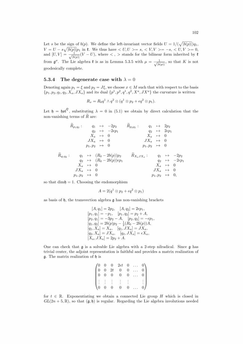
102

Let s be the sign of b(p). We define the left-invariant vector fields U = 1/(√|b(p)|)q1,

V = U − s√|b(p)|p1 in k. We thus have < U,U >= s, < V, V >= −s, < U, V >= 0,

and [U, V ] = 1√|b(p)|

(V − U), where < , > stands for the bilinear form inherited by k

from gσ. The Lie algebra k is as in Lemma 5.3.5 with µ = 1√|b(p)|

, so that K is not

geodesically complete.

5.3.4 The degenerate case with λ = 0

Denoting again p1 = ξ and p2 = Jξ, we choose x ∈M such that with respect to the basisp1, p2, q1, q2, Xa, JXa and its dual p1, p2, q1, q2, Xa, JXa the curvature is written

Rx = R0q1 ∧ q2 ⊗ (q1 ⊗ p2 + εq2 ⊗ p1).

Let h = hol∇, substituting λ = 0 in (5.1) we obtain by direct calculation that the

non-vanishing terms of R are:

Rp1q2 : q1 7→ −2p2

q2 7→ −2εp1

Xa 7→ 0JXa 7→ 0p1, p2 7→ 0

Rp2q1 : q1 7→ 2p2

q2 7→ 2εp1

Xa 7→ 0JXa 7→ 0p1, p2 7→ 0

Rq1q2 : q1 7→ (R0 − 2b(p))p2

q2 7→ (R0 − 2b(p))εp1

Xa 7→ 0JXa 7→ 0p1, p2 7→ 0

RXaJXa : q1 7→ −2p2

q2 7→ −2εp1

Xa 7→ 0JXa 7→ 0p1, p2 7→ 0,

so that dimh = 1. Choosing the endomorphism

A = 2(q1 ⊗ p2 + εq2 ⊗ p1)

as basis of h, the transvection algebra g has non-vanishing brackets

[A, q1] = 2p2, [A, q2] = 2εp1,[p1, q1] = −p1, [p1, q2] = p2 +A,[p2, q1] = −3p2 −A, [p2, q2] = −εp1,[q1, q2] = 2b(p)p2 − 1

2 (R0 − 2b(p))A,[q1, Xa] = Xa, [q1, JXa] = JXa,[q2, Xa] = JXa, [q2, JXa] = εXa,[Xa, JXa] = 2p2 +A.

One can check that g is a solvable Lie algebra with a 2-step nilradical. Since g hastrivial center, the adjoint representation is faithful and provides a matrix realization ofg. The matrix realization of h is

0 0 0 2εt 0 . . . 00 0 2t 0 0 . . . 00 0 0 0 0 . . . 0...

......

......

...0 0 0 0 0 . . . 0

for t ∈ R. Exponentiating we obtain a connected Lie group H which is closed inGL(2n + 5,R), so that (g, h) is regular. Regarding the Lie algebra involutions needed

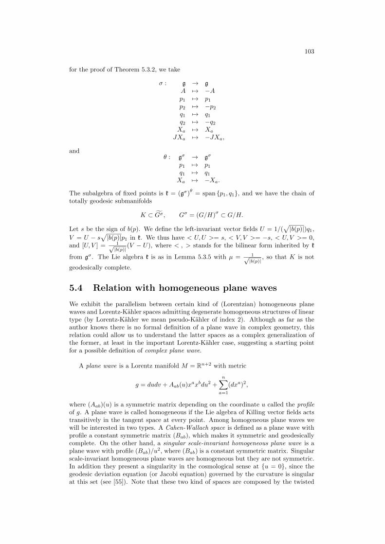
103

for the proof of Theorem 5.3.2, we take

σ : g → gA 7→ −Ap1 7→ p1

p2 7→ −p2

q1 7→ q1

q2 7→ −q2

Xa 7→ Xa

JXa 7→ −JXa,

andθ : gσ → gσ

p1 7→ p1

q1 7→ q1

Xa 7→ −Xa.

The subalgebra of fixed points is k = (gσ)θ

= span p1, q1, and we have the chain oftotally geodesic submanifolds

K ⊂ Gσ, Gσ = (G/H)σ ⊂ G/H.

Let s be the sign of b(p). We define the left-invariant vector fields U = 1/(√|b(p)|)q1,

V = U − s√|b(p)|p1 in k. We thus have < U,U >= s, < V, V >= −s, < U, V >= 0,

and [U, V ] = 1√|b(p)|

(V − U), where < , > stands for the bilinear form inherited by k

from gσ. The Lie algebra k is as in Lemma 5.3.5 with µ = 1√|b(p)|

, so that K is not

geodesically complete.

5.4 Relation with homogeneous plane waves

We exhibit the parallelism between certain kind of (Lorentzian) homogeneous planewaves and Lorentz-Kahler spaces admitting degenerate homogeneous structures of lineartype (by Lorentz-Kahler we mean pseudo-Kahler of index 2). Although as far as theauthor knows there is no formal definition of a plane wave in complex geometry, thisrelation could allow us to understand the latter spaces as a complex generalization ofthe former, at least in the important Lorentz-Kahler case, suggesting a starting pointfor a possible definition of complex plane wave.

A plane wave is a Lorentz manifold M = Rn+2 with metric

g = dudv +Aab(u)xaxbdu2 +

n∑a=1

(dxa)2,

where (Aab)(u) is a symmetric matrix depending on the coordinate u called the profileof g. A plane wave is called homogeneous if the Lie algebra of Killing vector fields actstransitively in the tangent space at every point. Among homogeneous plane waves wewill be interested in two types. A Cahen-Wallach space is defined as a plane wave withprofile a constant symmetric matrix (Bab), which makes it symmetric and geodesicallycomplete. On the other hand, a singular scale-invariant homogeneous plane wave is aplane wave with profile (Bab)/u

2, where (Bab) is a constant symmetric matrix. Singularscale-invariant homogeneous plane waves are homogeneous but they are not symmetric.In addition they present a singularity in the cosmological sense at u = 0, since thegeodesic deviation equation (or Jacobi equation) governed by the curvature is singularat this set (see [55]). Note that these two kind of spaces are composed by the twisted

104

product of a totally geodesic flat wave front and a 2-dimensional manifold containingtime and the direction of propagation. This 2-dimensional space gives the real geometricinformation of the total manifold and in particular it contains a null parallel vector field.They are all VSI, and the curvature information is contained in the profile Aab(u), sincethe only non-vanishing component of the curvature is given by

Ruaub = −Aab(u), a, b = 1, . . . , n.

Cahen-Wallach spaces are one of the possible indecomposable simply-connectedLorentzian symmetric spaces together with (R,−dt2), the de Sitter, and the anti deSitter spaces (see [15]). On the other hand, in [46] the following characterization isgiven.

Theorem 5.4.1 Let (M, g) be a connected pseudo-Riemannian manifold of dimensionn+ 2 admitting a degenerate homogeneous pseudo-Riemannian structure of linear type(see Subsection 4.2.1) with g(ξ, ξ) = 0. Then (M, g) is locally isometric to Rn+2 withmetric

ds2 = dudv +Babu2

xaxbdu2 +

n∑a=1

εa(dxa)2

for some symmetric matrix (Bab) and εa = ±1, a = 1, . . . , n.

Note that for Lorentzian signature this means that a manifold admitting a degeneratehomogeneous structure of linear type is locally a singular scale-invariant homogeneousplane wave. Conversely, it is easy to see that every singular scale-invariant homogeneousplane wave admits such a homogeneous structure with ξ = − 1

u∂v.

In the Lorentz-Kahler case, according to [33] there is only one possibility for a simply-connected, indecomposable (and not irreducible), symmetric space of complex dimension2 and signature (2, 2) with a null parallel complex vector field, that is a manifold withholonomy

holγ1=0,γ2=0n=0 = R

(i i−i −i

)in the notation of [33]. In order to get a plane wave structure we add a plane wave frontby considering a manifold (M, g, J) with holonomy holγ1=0,γ2=0

n=0 ⊕ 0n. Note that thisis the holonomy algebra in Proposition 5.2.4 for ε = −1.

Proposition 5.4.2 Let (M, g, J) be a locally symmetric Lorentz-Kahler manifold ofdimension 2n + 4, n ≥ 0, with holonomy holγ1=0,γ2=0

n=0 ⊕ 0n. Then the metric g islocally of the form

g = dw1dz1 + dw2dz2 + b(dw1dw1 + dw2dw2) +

n∑a=1

(dxadxa + dyadya), (5.29)

where the function b only depends on w1 and w2 and satisfies

∆b = b0, b0 ∈ R− 0.

Proof. Looking at the holonomy representation, there are two parallel isotropic (real)vector fields Z and JZ on M . Let α1 = g(·, Z) and α2 = −α1 J , consider the complexform α = α1 + iα2. Since ∇Z = 0 = ∇JZ, we have ∇α = 0, hence in particularα is holomorphic and closed. This means that locally there is a holomorphic functionw : U → C such that dw = α. Since dw is non-zero at some point and it is parallel,we have that dw is nowhere vanishing. Hence if the set w−1(λ), λ ∈ C, is non-emptythen it defines a complex hypersurface in U . Let p ∈M and let q1 ∈ TpM be such thatg(Zp, q1) = 1 with g(q1, q1) 6= 0. The subspace E = SpanZp, JZp, q1Jq1 is invariant

105

by holonomy, hence so is E⊥. In fact, the holonomy action is trivial on E⊥. This impliesthat there are parallel vector fields Ei, JEi, i = 1, . . . , n, which are an orthonormal basisof E⊥ at every point. In addition, it is easy to see that Z, JZ,Ei, JEi are always tangentto the hypersurfaces w−1(λ). We can thus take coordinates w1, w2, z1, z2, xa, ya withw = w1 + iw2, ∂z1 = Z, ∂z2 = JZ, ∂xi = Ei and ∂yi = JEi, and such that

g = dw1dz1 + dw2dz2 + b(dw1dw1 + dw2dw2) +

n∑a=1

(dxadxa + dyadya).

In addition, the only non-zero element of the curvature tensor field is

R∂w1∂w2∂w1∂w2 =1

2∆b,

where ∆ stands for the Laplace operator with respect to the variables (w1, w2). Thecondition of being locally symmetric is then

∇R = 0 ⇔ ∆b = b0,

for b0 ∈ R− 0.

The previous Proposition suggests to consider the pseudo-Kahler manifold (C2+n, g)with g as in (5.29) as a natural Lorentz-Kahler analogue to Cahen-Wallach spaces. Notethat equation ∆b = b0 admits singular solutions. Nevertheless, as Cahen-Wallach spacesare simply-connected, in order to have an actual analogue we only consider non-singularfunctions b, so that (C2+n, g) is complete.

On the other hand, since Lorentzian singular scale-invariant homogeneous planewaves are characterized by degenerate pseudo-Riemannian homogeneous structures oflinear type, from Propositions 5.2.5 and 5.2.6, the natural analogues to these spacesare Lorentz-Kahler manifolds with degenerate homogeneous pseudo-Kahler structuresof linear type. More precisely, the spaces (Cn+2−‖w‖λ = 0, g) with ‖w‖λ as in (5.24),g as in (5.25) with ε = −1 and signature (2, 2+2n), and (Cn+2, g) with g given in (5.29),are composed by the twisted product of a flat and totally geodesic complex manifoldand a 2-dimensional complex manifold containing a null parallel complex vector field.Moreover, expression (5.25) and (5.29) are the same except for the function b, whichhas a different Laplacian in each case. As a straight forward computation shows, thecurvature tensor of both metrics is

R =1

2∆b(dw1 ∧ dw2)⊗ (dw1 ∧ dw2),

whence all the curvature information is contained in the Laplacian of the function b.For this reason, analogously to Lorentz plane waves, we call ∆b the profile of the metric.

It is worth noting that in the Lorentz case one goes from Cahen-Wallach spaces tosingular scale-invariant homogeneous plane waves by making the profile be singular witha term 1/u2. Doing so, the space is no longer geodesically complete and a cosmologicalsingularity at u = 0 is created. In the same way, in the Lorentz-Kahler case onegoes from metric (5.29) to (5.25) by making the profile be singular with a term 1/‖w‖4λ,and again one transforms a geodesically complete space into a geodesically incompletespace creating a singularity at ‖w‖λ = 0. Finally, we also note that all these metricsare VSI. This reinforces the parallelism and exhibits a close relation between these twocouples of spaces.

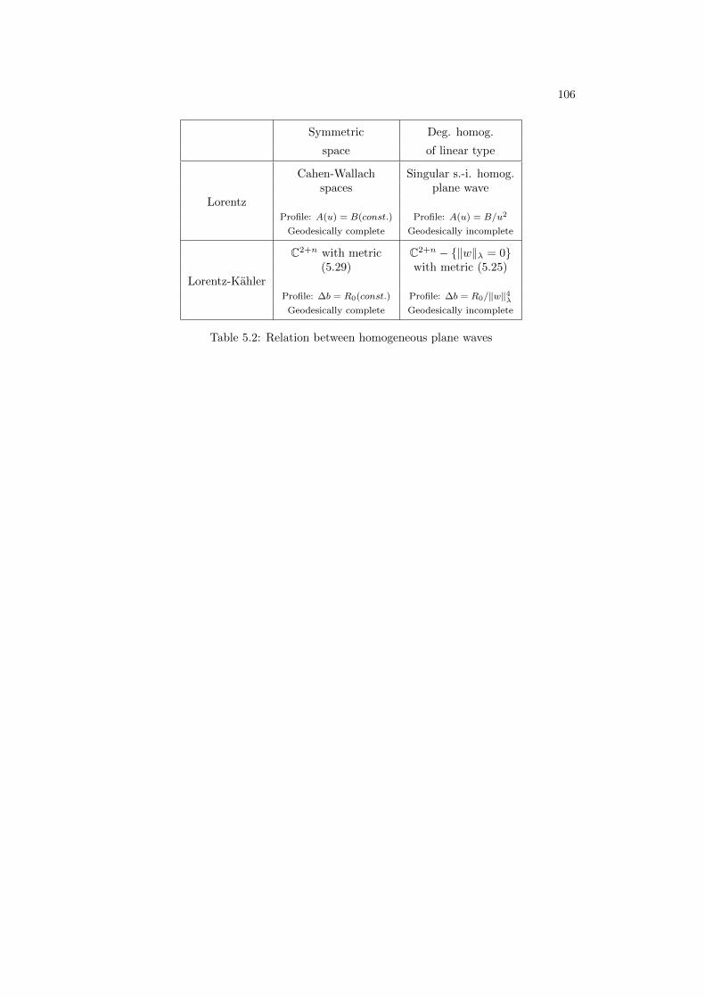
106

Symmetric Deg. homog.

space of linear type

Lorentz

Cahen-Wallach Singular s.-i. homog.spaces plane wave

Profile: A(u) = B(const.) Profile: A(u) = B/u2

Geodesically complete Geodesically incomplete

Lorentz-Kahler

C2+n with metric C2+n − ‖w‖λ = 0(5.29) with metric (5.25)

Profile: ∆b = R0(const.) Profile: ∆b = R0/‖w‖4λGeodesically complete Geodesically incomplete

Table 5.2: Relation between homogeneous plane waves

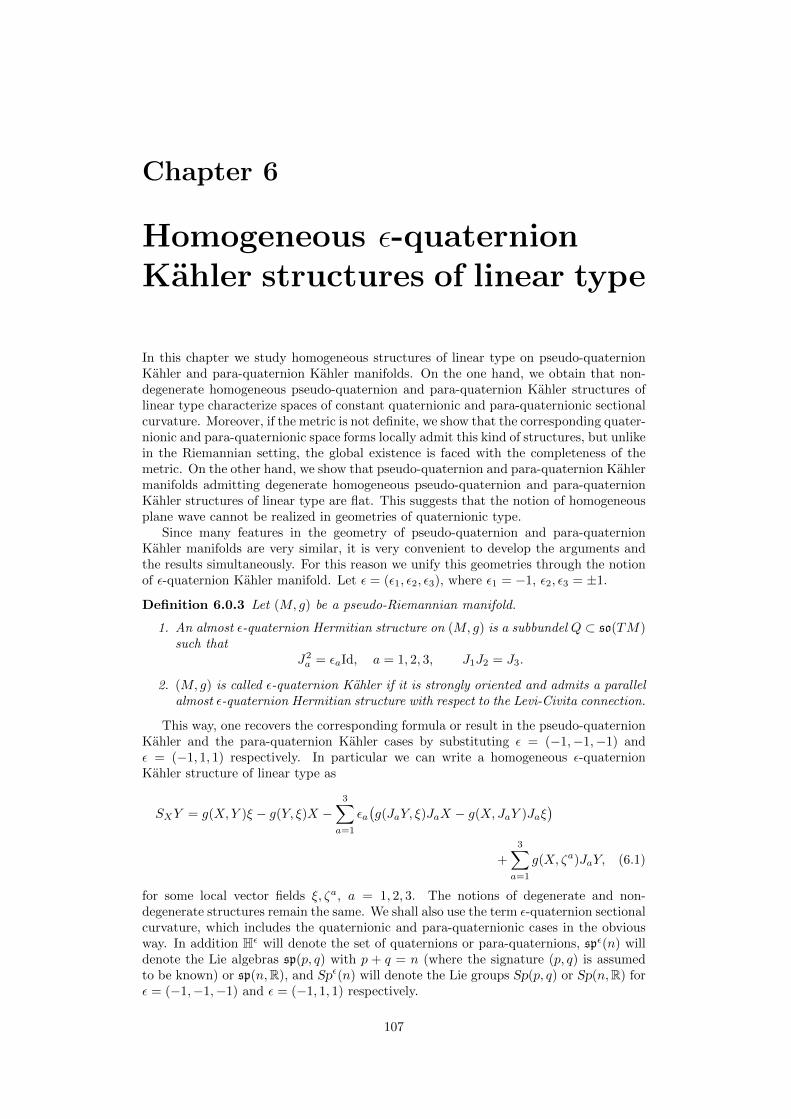
Chapter 6

Homogeneous ε-quaternionKahler structures of linear type

In this chapter we study homogeneous structures of linear type on pseudo-quaternionKahler and para-quaternion Kahler manifolds. On the one hand, we obtain that non-degenerate homogeneous pseudo-quaternion and para-quaternion Kahler structures oflinear type characterize spaces of constant quaternionic and para-quaternionic sectionalcurvature. Moreover, if the metric is not definite, we show that the corresponding quater-nionic and para-quaternionic space forms locally admit this kind of structures, but unlikein the Riemannian setting, the global existence is faced with the completeness of themetric. On the other hand, we show that pseudo-quaternion and para-quaternion Kahlermanifolds admitting degenerate homogeneous pseudo-quaternion and para-quaternionKahler structures of linear type are flat. This suggests that the notion of homogeneousplane wave cannot be realized in geometries of quaternionic type.

Since many features in the geometry of pseudo-quaternion and para-quaternionKahler manifolds are very similar, it is very convenient to develop the arguments andthe results simultaneously. For this reason we unify this geometries through the notionof ε-quaternion Kahler manifold. Let ε = (ε1, ε2, ε3), where ε1 = −1, ε2, ε3 = ±1.

Definition 6.0.3 Let (M, g) be a pseudo-Riemannian manifold.

1. An almost ε-quaternion Hermitian structure on (M, g) is a subbundel Q ⊂ so(TM)such that

J2a = εaId, a = 1, 2, 3, J1J2 = J3.

2. (M, g) is called ε-quaternion Kahler if it is strongly oriented and admits a parallelalmost ε-quaternion Hermitian structure with respect to the Levi-Civita connection.

This way, one recovers the corresponding formula or result in the pseudo-quaternionKahler and the para-quaternion Kahler cases by substituting ε = (−1,−1,−1) andε = (−1, 1, 1) respectively. In particular we can write a homogeneous ε-quaternionKahler structure of linear type as

SXY = g(X,Y )ξ − g(Y, ξ)X −3∑a=1

εa(g(JaY, ξ)JaX − g(X, JaY )Jaξ

)+

3∑a=1

g(X, ζa)JaY, (6.1)

for some local vector fields ξ, ζa, a = 1, 2, 3. The notions of degenerate and non-degenerate structures remain the same. We shall also use the term ε-quaternion sectionalcurvature, which includes the quaternionic and para-quaternionic cases in the obviousway. In addition Hε will denote the set of quaternions or para-quaternions, spε(n) willdenote the Lie algebras sp(p, q) with p + q = n (where the signature (p, q) is assumedto be known) or sp(n,R), and Spε(n) will denote the Lie groups Sp(p, q) or Sp(n,R) forε = (−1,−1,−1) and ε = (−1, 1, 1) respectively.

107

108

6.1 Characterizing homogeneous ε-quaternionKahler structures of linear type

Theorem 6.1.1 Let (M, g,Q) be a connected ε-quaternion Kahler manifold of dimen-sion 4n > 8 admitting a homogeneous ε-quaternion Kahler structure of linear type S.If S is non-degenerate, then (M, g,Q) has constant ε-quaternion sectional curvature−4g(ξ, ξ), and ζa = 0 for a = 1, 2, 3. If S is degenerate then (M, g,Q) is flat.

Proof. By Propositions 1.2.21 and 1.2.25 we decompose the curvature tensor field of(M, g,Q) as R = νqR

0 +Rspε(n), where Rspε(n) is a curvature tensor field of type spε(n).Recall that the space of algebraic curvature tensors Rspε(n) is [S4E] with E = C2n forε = (−1,−1,−1), and S4E with E = R2n for ε = (−1, 1, 1). Since R0 is Spε(n)Spε(1)-invariant, the covariant derivative ∇R0 vanishes. Moreover, for every vector field X,SX acts as an element of spε(n) + spε(1), whence S · R0 = 0. Using that ∇R = 0 and

∇ = ∇− S we have

0 = ∇R = νq∇R0 + ∇Rspε(n) = ∇Rspε(n) − S ·Rspε(n).

Writing T ∗M ⊗ (spε(n) + spε(1)) = T ∗M ⊗ spε(n) + T ∗M ⊗ spε(1) we can decomposeS = SE + SH , and hence SH ·Rspε(n) = 0. We thus obtain

∇R = ∇Rspε(n) = SE ·Rspε(n),

which we can write as

(∇XR)Y ZWU = −Rspε(n)SXY ZWU −R

spε(n)Y SXZWU −R

spε(n)Y ZSXWU −R

spε(n)Y ZWSXU

. (6.2)

Taking the cyclic sum in X,Y, Z and applying Bianchi identities we obtain

0 = SXYZ

2g(X, ξ)R

spε(n)Y ZWU + g(X,W )R

spε(n)Y ZξU + g(X,U)R

spε(n)Y ZWξ

+ 2∑a

εa(g(X, JaY )R

spε(n)JaξZWU + g(X, JaW )R

spε(n)Y ZJaξU

+ g(X,JaU)Rspε(n)Y ZWJaξ

).

Contracting the previous formula with respect to X and W , and taking into accountthat Rspε(n) is traceless we obtain

(4n+ 2)Rspε(n)Y ZξU = 0,

for every vector fields Z, Y, U . Expanding the expression of S in (6.2) and using theprevious formula we arrive at

0 = SXYZ

θ(X)Rspε(n)Y ZWU ,

where θ = ξ[, or equivalently

0 = θ ∧Rspε(n)WU . (6.3)

Noting that Rspε(n) satisfies the symmetries Rspε(n)XJaYWU +R

spε(n)JaXYWU = 0, a = 1, 2, 3, we

also have0 = (θ Ja) ∧Rspε(n)

WU = 0, a = 1, 2, 3. (6.4)

It is easy to see that a curvature tensor of type spε(n) satisfying equations (6.3) and(6.4) must vanish. Therefore we conclude that R = νqR

0.

109

Now, making use of ∇S = 0 together with (6.1), and taking into account (4.6) and(4.11) we have that

0 = g(X,Y )∇Zξ − g(∇Zξ, Y )X −∑a

εa(g(∇Zξ, JaY )JaX + g(X, JaY )Ja∇Zξ)

+∑a

g(X, ∇Zζa −∑b

dba(Z)ζb)JaY,

where (dba) is a matrix of 1-forms sitting in spε(1). Taking X ∈ (Hεξ)⊥ with g(X,X) 6=0, and multiplying by X in the previous formula we obtain that

∇Zξ = 0. (6.5)

Hence∇Zζa =

∑b

dbaζb, a = 1, 2, 3. (6.6)

From (6.5), (4.6) and (4.11) we compute

∇XJaξ =∑b

dab(X)Jbξ + g(X, Jaξ)ξ

−∑b

εb(g(ξ, JbJaξ)JbX − g(X,JbJaX)Jbξ) +∑b

g(X, ζb)JbJaξ. (6.7)

On the other hand

RXY ξ = −∇X∇Y ξ +∇Y∇Xξ +∇[X,Y ]ξ

= −g(Y,∇Xξ)ξ − g(Y, ξ)∇Xξ + g(X,∇Y ξ)ξ + g(X, ξ)∇Y ξ

−∑a

εa(g(Y,∇XJaξ)Jaξ + g(Y, Jaξ)∇XJaξ

− g(X,∇Y Jaξ)Jaξ − g(X, Jaξ)∇Y Jaξ)

+∑a

−g(Y,∇Xζa)Jaξ − g(Y, ζa)∇XJaξ

+ g(X,∇Y ζa)Jaξ + g(X, ζa)∇Y Jaξ.

(6.8)

If S is non-degenerate, taking X,Y ∈ (Hεξ)⊥, we have g(RXY ξ,X) = 0 from R = νqR0

on the one hand, and

g(RXY ξ,X) =∑a

g(X, ζa)g(ξ, ξ)g(JaY,X)

from (6.8) on the other. Moreover, for Y = JbX it reduces to

g(RXJbXξ,X) = −εbg(ξ, ξ)g(X, ζb)g(X,X).

This implies that g(X, ζb) = 0, so that

ζb ∈ Hεξ, b = 1, 2, 3.

Recalling (6.5) we have that g(ξ,∇Y ξ) = 0. Applying this and (4.6) and (4.11) to (6.8)with X = ξ and Y ∈ (Hεξ)⊥ we obtain

g(Y,∇Y Jaξ) = 0, g(Y,∇Y ζa) = 0, g(ξ,∇Y ζa) = 0,

g(Y,∇ξJaξ) = g(Y, Ja∇ξξ) +∑b

g(Y, bab(ξ)Jbξ) = 0,

110

g(Y,∇Y Jaξ) = g(ξ, Ja∇Y ξ) +∑b

g(ξ, babJbξ) = 0.

Hence

RξY ξ = g(ξ, ξ)∇Y ξ +∑a

g(ξ, ζa)∇Y Jaξ

= −g(ξ, ξ)2Y −∑a

g(ξ, ζa)∑b

εbg(JbJaξ, ξ)JbY

= −g(ξ, ξ)2Y −∑a

g(ξ, ζa)g(ξ, ξ)JaY.

Comparing with RξY ξ = νqR0ξY ξ = νqg(ξ, ξ)Y we deduce that νq = −g(ξ, ξ) and

g(ξ, ζa) = 0. Finally we take again X,Y ∈ (Hεξ)⊥ in (6.8) obtaining

RXY ξ = −g(Y,∇Xξ)ξ + g(X,∇Y ξ)ξ

−∑a

εa(g(Y,∇XJaξ)Jaξ − g(X,∇Y Jaξ)Jaξ)

+∑a

−g(Y,∇Xζa)Jaξ + g(X,∇Y ζa)Jaξ.

Taking into account (6.6), the previous formula reads

RXY ξ = 2∑a

εag(Y, JaX)g(ξ, ξ)Jaξ + 2∑a,b

εbg(Y, JbX)g(ξ, Jbζa)Jaξ,

and comparing with

RXY ξ = νqR0XY ξ = −2

∑a

εag(ξ, ξ)g(X, JaY )Jaξ

we haveg(Jbζ

a, ξ) = 0, a, b = 1, 2, 3.

This in conjunction with ζa ∈ (Hεξ)⊥ and g(ζa, ξ) = 0 gives

ζa = 0, a = 1, 2, 3.

Finally, if S is degenerate, we apply ∇ξ = 0 and ∇Ja =∑b cabJb to (6.8) obtaining

that RXY ξ ∈ spanξ, J1ξ, J2ξ, J3ξ. Comparing this with RXY ξ = νqR0XY ξ we deduce

that νq = 0, so that R = 0.

Remark 6.1.2 In the non-degenerate case, for ε = (−1,−1,−1), if g(ξ, ξ) > 0 thenc = −4g(ξ, ξ) < 0, so that spaces with negative definite metric and constant nega-tive quaternionic sectional curvature cannot admit non-degenerate homogeneous pseudo-quaternion structures of linear type. Similarly, if g(ξ, ξ) < 0 then c > 0, so that spaceswith positive definite metric and constant positive quaternionic sectional curvature arealso excluded.

Remark 6.1.3 For ε = −1, if g(ξ, ξ) > 0 then c = −4g(ξ, ξ) < 0, so that spaces withnegative definite metric and constant negative holomorphic sectional curvature cannotadmit non-degenerate homogeneous pseudo-Kahler structures of linear type. Similarly, ifg(ξ, ξ) < 0 then c > 0, so that spaces with positive definite metric and constant positiveholomorphic sectional curvature are also excluded.

From the arguments used in the proof of Theorem 6.1.1, the following result isevident.

Proposition 6.1.4 Let (M, g, J1, J2, J3) be a pseudo-hyper-Kahler (resp. para-hyper-Kahler) manifold admitting a homogeneous pseudo-hyper-Kahler (para-hyper-Kahler)structure of linear type. Then (M, g, J1, J2, J3) is flat.

111

6.2 Infinitesimal models, homogeneous models andcompleteness

Recall the definition of infinitesimal model, transvection algebra and homogeneousmodel associated to a homogeneous structure (Section 2.3). Since by Theorem 6.1.1,degenerate homogeneous ε-quaternion Kahler structures of linear type only exist for flatmetrics, we will be only interested in non-degenerate structures. The aim of this sectionis to prove the following results.

Theorem 6.2.1 With the exception of HPn0 and HHnn, the indefinite ε-quaternion space

forms HPns , HHns and HPn locally admit a non-degenerate homogeneous ε-quaternion

Kahler structure of linear type.

Theorem 6.2.2 Let (M, g,Q) be a connected and simply-connected ε-quaternion Kahlermanifold with dimM > 8 admitting a non-degenerate homogeneous ε-quaternion Kahlerstructure of linear type. If g is not definite then (M, g,Q) is not complete.

Remark 6.2.3 Note that Theorem 6.2.2 implies that the indefinite ε-quaternion spaceforms HPnp , HHn

p and HPn do not admit a globally defined non-degenerate homogeneousε-quaternion Kahler structure of linear type except for HPnn and HHn

0 .

In order to prove Theorems 6.2.1 and 6.2.2, we can adapt in a straightforward waythe procedure used to prove Theorems 5.3.1 and 5.3.2 in Section 5.3. In fact, the onlydifference is that, by Remark 1.2.22, we will need only consider the spaces HHn

p and

HPn, since by Theorem 5.1.2 our spaces of linear type are locally ±-isometric to one ofthese models. In addition, the expression of this spaces as Isom/Isot are given by (1.4)and (1.6) respectively. We thus just have to specify all the components involved in thatprocedure for each case. Due to differences we treat them separately.

6.2.1 The para-quaternion Kahler case

During this subsection H denotes the set of para-quaternions with imaginary units i, j, k.Using (6.1) we compute

RSXYW = −g(ξ, ξ)g(X,W )Y − g(Y,W )X

+∑a

εa(g(X, JaW )JaY − g(Y, JaW )JaX)

− 2∑a

εa(g(ξ, JaW )g(X, JaY )ξ + g(ξ,W )g(X, JaY )Jaξ)

+ 2∑a

(g(X,JaY )g(ξ, JcW )Jbξ − g(X,JaY )g(ξ, JbW )Jcξ),

where (a, b, c) is a cyclic permutation of (1, 2, 3), and (ε1, ε2, ε3) = (−1, 1, 1). From

R = R−RS and R = −g(ξ, ξ)R0, we obtain

RXYW = −2∑a

εag(ξ, ξ)g(X, JaY )JaW

+ 2∑a

g(X,JaY )(εag(ξ, JaW )ξ + εag(ξ,W )Jaξ − g(ξ, JcW )Jbξ

+ g(ξ, JbW )Jcξ).

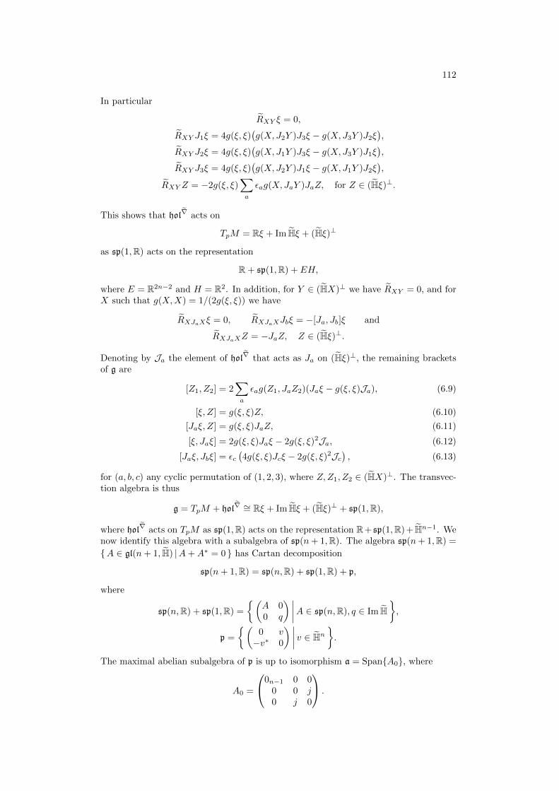
112

In particular

RXY ξ = 0,

RXY J1ξ = 4g(ξ, ξ)(g(X, J2Y )J3ξ − g(X, J3Y )J2ξ

),

RXY J2ξ = 4g(ξ, ξ)(g(X, J1Y )J3ξ − g(X, J3Y )J1ξ

),

RXY J3ξ = 4g(ξ, ξ)(g(X, J2Y )J1ξ − g(X, J1Y )J2ξ

),

RXY Z = −2g(ξ, ξ)∑a

εag(X, JaY )JaZ, for Z ∈ (Hξ)⊥.

This shows that hol∇ acts on

TpM = Rξ + Im Hξ + (Hξ)⊥

as sp(1,R) acts on the representation

R+ sp(1,R) + EH,

where E = R2n−2 and H = R2. In addition, for Y ∈ (HX)⊥ we have RXY = 0, and forX such that g(X,X) = 1/(2g(ξ, ξ)) we have

RXJaXξ = 0, RXJaXJbξ = −[Ja, Jb]ξ and

RXJaXZ = −JaZ, Z ∈ (Hξ)⊥.

Denoting by Ja the element of hol∇ that acts as Ja on (Hξ)⊥, the remaining bracketsof g are

[Z1, Z2] = 2∑a

εag(Z1, JaZ2)(Jaξ − g(ξ, ξ)Ja), (6.9)

[ξ, Z] = g(ξ, ξ)Z, (6.10)

[Jaξ, Z] = g(ξ, ξ)JaZ, (6.11)

[ξ, Jaξ] = 2g(ξ, ξ)Jaξ − 2g(ξ, ξ)2Ja, (6.12)

[Jaξ, Jbξ] = εc(4g(ξ, ξ)Jcξ − 2g(ξ, ξ)2Jc

), (6.13)

for (a, b, c) any cyclic permutation of (1, 2, 3), where Z,Z1, Z2 ∈ (HX)⊥. The transvec-tion algebra is thus

g = TpM + hol∇ ∼= Rξ + Im Hξ + (Hξ)⊥ + sp(1,R),

where hol∇ acts on TpM as sp(1,R) acts on the representation R+ sp(1,R)+ Hn−1. Wenow identify this algebra with a subalgebra of sp(n+ 1,R). The algebra sp(n+ 1,R) =

A ∈ gl(n+ 1, H) |A+A∗ = 0 has Cartan decomposition

sp(n+ 1,R) = sp(n,R) + sp(1,R) + p,

where

sp(n,R) + sp(1,R) =

(A 00 q

) ∣∣∣∣A ∈ sp(n,R), q ∈ Im H,

p =

(0 v−v∗ 0

) ∣∣∣∣ v ∈ Hn.The maximal abelian subalgebra of p is up to isomorphism a = SpanA0, where

A0 =

0n−1 0 00 0 j0 j 0

.

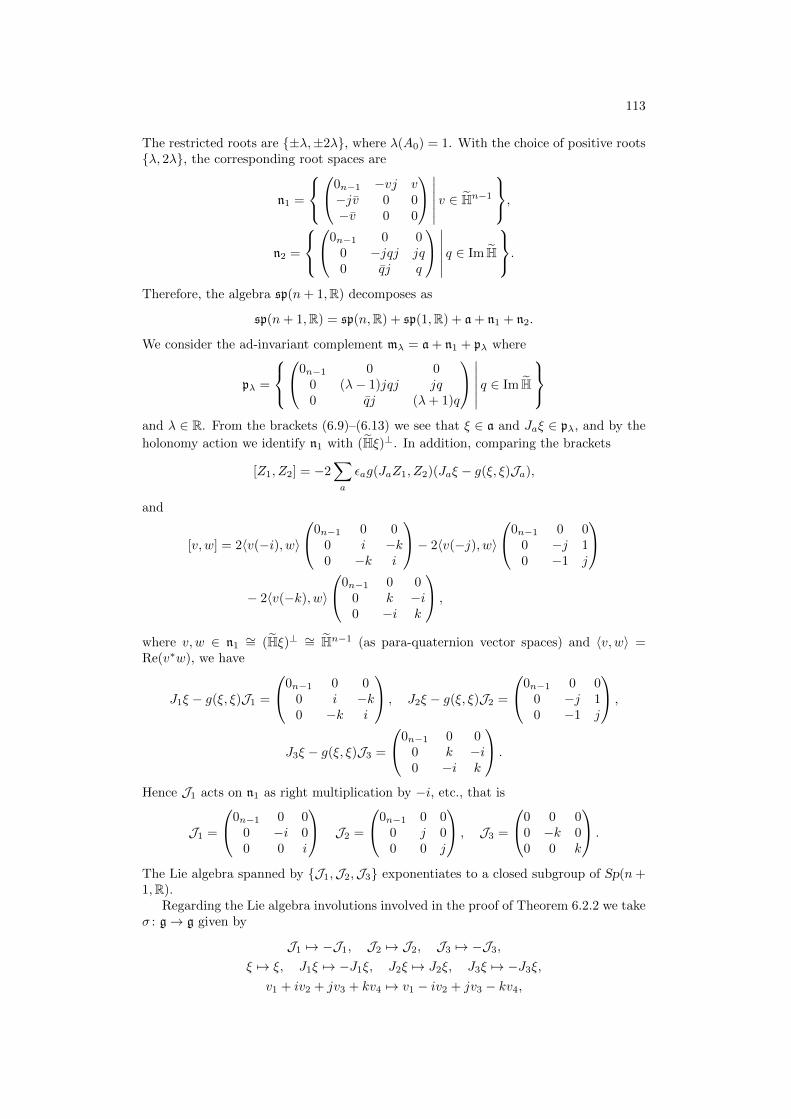
113

The restricted roots are ±λ,±2λ, where λ(A0) = 1. With the choice of positive rootsλ, 2λ, the corresponding root spaces are

n1 =

0n−1 −vj v−jv 0 0−v 0 0

∣∣∣∣∣∣ v ∈ Hn−1

,n2 =

0n−1 0 0

0 −jqj jq0 qj q

∣∣∣∣∣∣ q ∈ Im H

.Therefore, the algebra sp(n+ 1,R) decomposes as

sp(n+ 1,R) = sp(n,R) + sp(1,R) + a + n1 + n2.

We consider the ad-invariant complement mλ = a + n1 + pλ where

pλ =

0n−1 0 0

0 (λ− 1)jqj jq0 qj (λ+ 1)q

∣∣∣∣∣∣ q ∈ Im H

and λ ∈ R. From the brackets (6.9)–(6.13) we see that ξ ∈ a and Jaξ ∈ pλ, and by the

holonomy action we identify n1 with (Hξ)⊥. In addition, comparing the brackets

[Z1, Z2] = −2∑a

εag(JaZ1, Z2)(Jaξ − g(ξ, ξ)Ja),

and

[v, w] = 2〈v(−i), w〉

0n−1 0 00 i −k0 −k i

− 2〈v(−j), w〉

0n−1 0 00 −j 10 −1 j

− 2〈v(−k), w〉

0n−1 0 00 k −i0 −i k

,

where v, w ∈ n1∼= (Hξ)⊥ ∼= Hn−1 (as para-quaternion vector spaces) and 〈v, w〉 =

Re(v∗w), we have

J1ξ − g(ξ, ξ)J1 =

0n−1 0 00 i −k0 −k i

, J2ξ − g(ξ, ξ)J2 =

0n−1 0 00 −j 10 −1 j

,

J3ξ − g(ξ, ξ)J3 =

0n−1 0 00 k −i0 −i k

.

Hence J1 acts on n1 as right multiplication by −i, etc., that is

J1 =

0n−1 0 00 −i 00 0 i

J2 =

0n−1 0 00 j 00 0 j

, J3 =

0 0 00 −k 00 0 k

.

The Lie algebra spanned by J1,J2,J3 exponentiates to a closed subgroup of Sp(n+1,R).

Regarding the Lie algebra involutions involved in the proof of Theorem 6.2.2 we takeσ : g→ g given by

J1 7→ −J1, J2 7→ J2, J3 7→ −J3,

ξ 7→ ξ, J1ξ 7→ −J1ξ, J2ξ 7→ J2ξ, J3ξ 7→ −J3ξ,

v1 + iv2 + jv3 + kv4 7→ v1 − iv2 + jv3 − kv4,

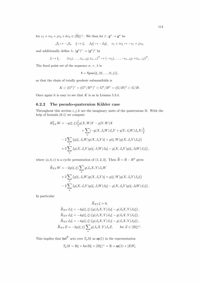
114

for v1 + iv2 + jv3 + kv4 ∈ (Hξ)⊥. We then let τ : gσ → gσ be

J2 7→ −J2, ξ 7→ ξ, J2ξ 7→ −J2ξ, v1 + iv2 7→ −v1 + jv2,

and additionally define λ : (gσ)τ → (gσ)τ by

ξ 7→ ξ, (v1j, . . . , vn−2j, vn−1)T 7→ (−v1j, . . . ,−vn−2j,+vn−1j)T ,

The fixed point set of the sequence σ, τ , λ is

k = Spanξ, (0, . . . , 0, j),

so that the chain of totally geodesic submanifolds is

K ⊂ (Gσ)τ = (Gσ/Hσ)τ ⊂ Gσ/Hσ = (G/H)σ ⊂ G/H.

Once again it is easy to see that K is as in Lemma 5.3.4.

6.2.2 The pseudo-quaternion Kahler case

Throughout this section i, j, k are the imaginary units of the quaternions H. With thehelp of formula (6.1) we compute

RSXYW = −g(ξ, ξ)g(X,W )Y − g(Y,W )X

+∑a

(−g(X,JaW )JaY + g(Y, JaW )JaX)

− 2∑a

g(ξ, JaW )g(X, JaY )ξ + g(ξ,W )g(X,JaY )Jaξ

+ 2∑a

g(X, JaY )g(ξ, JcW )Jbξ − g(X, JaY )g(ξ, JbW )Jcξ ,

where (a, b, c) is a cyclic permutation of (1, 2, 3). Then R = R−RS gives

RXYW = −2g(ξ, ξ)∑a

g(JaX,Y )JaW

+ 2∑a

g(ξ, JaW )g(X, JaY )ξ + g(ξ,W )g(X, JaY )Jaξ

− 2∑a

g(X, JaY )g(ξ, JcW )Jbξ − g(X, JaY )g(ξ, JbW )Jcξ .

In particular

RXY ξ = 0,

RXY J1ξ = −4g(ξ, ξ) g(J3X,Y )J2ξ − g(J2X,Y )J3ξ ,

RXY J2ξ = −4g(ξ, ξ) g(J1X,Y )J3ξ − g(J3X,Y )J1ξ ,

RXY J3ξ = −4g(ξ, ξ) g(J2X,Y )J1ξ − g(J1X,Y )J2ξ ,

RXY Z = −2g(ξ, ξ)∑a

g(JaX,Y )JaZ, for Z ∈ (Hξ)⊥.

This implies that hol∇ acts over TpM as sp(1) in the representation

TpM = Rξ + ImHξ + (Hξ)⊥ = R+ sp(1) + [EH],

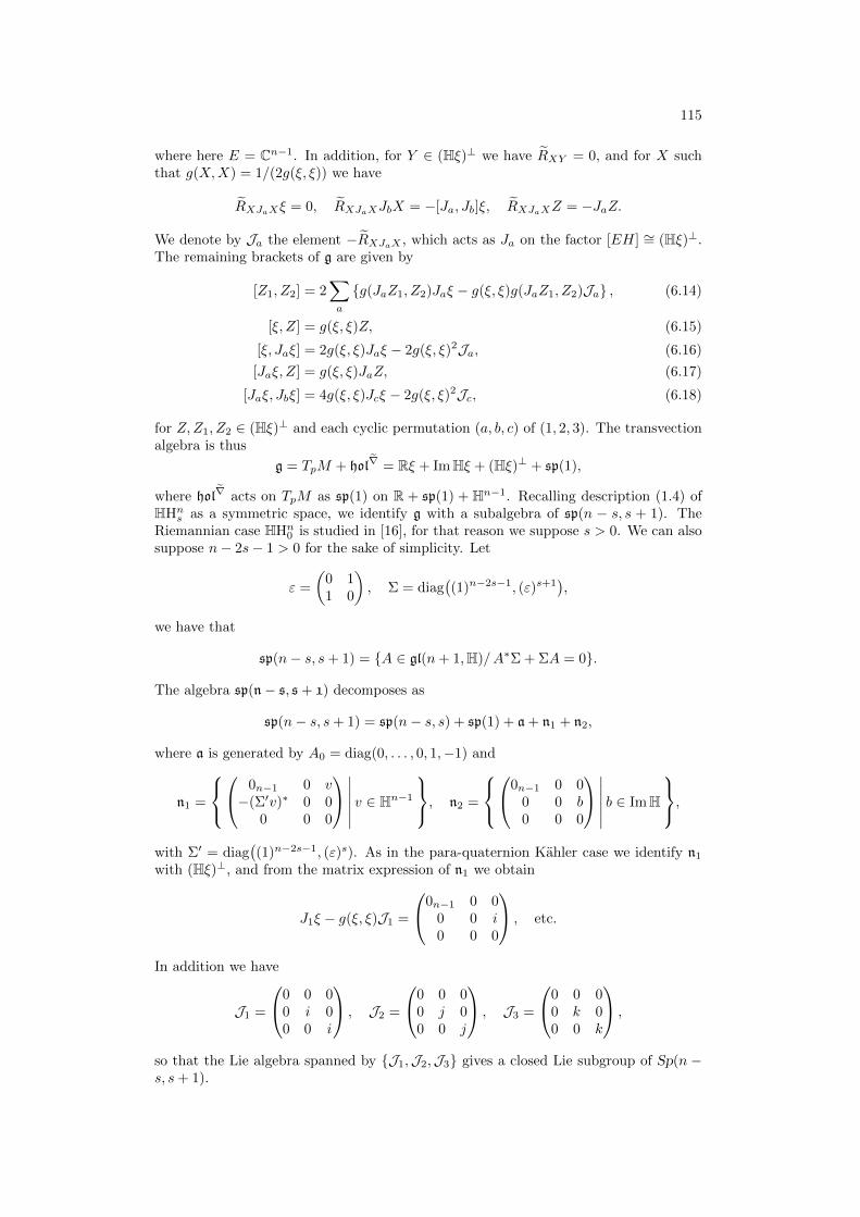
115

where here E = Cn−1. In addition, for Y ∈ (Hξ)⊥ we have RXY = 0, and for X suchthat g(X,X) = 1/(2g(ξ, ξ)) we have

RXJaXξ = 0, RXJaXJbX = −[Ja, Jb]ξ, RXJaXZ = −JaZ.

We denote by Ja the element −RXJaX , which acts as Ja on the factor [EH] ∼= (Hξ)⊥.The remaining brackets of g are given by

[Z1, Z2] = 2∑a

g(JaZ1, Z2)Jaξ − g(ξ, ξ)g(JaZ1, Z2)Ja , (6.14)

[ξ, Z] = g(ξ, ξ)Z, (6.15)

[ξ, Jaξ] = 2g(ξ, ξ)Jaξ − 2g(ξ, ξ)2Ja, (6.16)

[Jaξ, Z] = g(ξ, ξ)JaZ, (6.17)

[Jaξ, Jbξ] = 4g(ξ, ξ)Jcξ − 2g(ξ, ξ)2Jc, (6.18)

for Z,Z1, Z2 ∈ (Hξ)⊥ and each cyclic permutation (a, b, c) of (1, 2, 3). The transvectionalgebra is thus

g = TpM + hol∇ = Rξ + ImHξ + (Hξ)⊥ + sp(1),

where hol∇ acts on TpM as sp(1) on R + sp(1) + Hn−1. Recalling description (1.4) ofHHn

s as a symmetric space, we identify g with a subalgebra of sp(n − s, s + 1). TheRiemannian case HHn

0 is studied in [16], for that reason we suppose s > 0. We can alsosuppose n− 2s− 1 > 0 for the sake of simplicity. Let

ε =

(0 11 0

), Σ = diag

((1)n−2s−1, (ε)s+1

),

we have that

sp(n− s, s+ 1) = A ∈ gl(n+ 1,H)/A∗Σ + ΣA = 0.

The algebra sp(n− s, s + 1) decomposes as

sp(n− s, s+ 1) = sp(n− s, s) + sp(1) + a + n1 + n2,

where a is generated by A0 = diag(0, . . . , 0, 1,−1) and

n1 =

0n−1 0 v−(Σ′v)∗ 0 0

0 0 0

∣∣∣∣∣∣ v ∈ Hn−1

, n2 =

0n−1 0 0

0 0 b0 0 0

∣∣∣∣∣∣ b ∈ ImH

,with Σ′ = diag

((1)n−2s−1, (ε)s). As in the para-quaternion Kahler case we identify n1

with (Hξ)⊥, and from the matrix expression of n1 we obtain

J1ξ − g(ξ, ξ)J1 =

0n−1 0 00 0 i0 0 0

, etc.

In addition we have

J1 =

0 0 00 i 00 0 i

, J2 =

0 0 00 j 00 0 j

, J3 =

0 0 00 k 00 0 k

,

so that the Lie algebra spanned by J1,J2,J3 gives a closed Lie subgroup of Sp(n −s, s+ 1).

116

For the Lie algebra involutions involved in the proof of Theorem 6.2.2 we finally takeσ : g→ g given by

J1 7→ J1, J2 7→ −J2, J3 7→ −J3

ξ 7→ ξ, J1ξ 7→ J1ξ, J2ξ 7→ −J2ξ, J3ξ 7→ −J3ξ

v1 + iv2 + jv3 + kv4 7→ v1 + iv2 − jv3 − kv4,

for v1 + iv2 + jv3 + kv4 ∈ (Hξ)⊥. Then we put τ : gσ → gσ to be

J1 7→ −J1, ξ 7→ ξ, J1ξ 7→ −J1ξ, v1 + iv2 7→ v1 − iv2,

and define λ : (gσ)τ → (gσ)τ by

ξ 7→ ξ, (v1, . . . , vn−2, vn−1)T 7→ (−v1, . . . ,−vn−1,−vn−2)T .

This leads to the chain of totally geodesic submanifolds

K = ((Gσ)τ )λ ⊂ (Gσ)τ = (Gσ/Hσ)τ ⊂ Gσ/Hσ = (G/H)σ ⊂ G/H,

with K as in Lemma 5.3.4, and so incomplete.

Chapter 7

Reduction of homogeneousstructures

Symmetries represent a classical tool in reduction schemes intimately related with dif-ferent topics as systems of differential equations, variational principles, symplectic orother geometric structures, etc. In particular, reduction is recurrently applied in thesetting of homogeneous spaces. The goal of this chapter is the study of the behaviourof homogeneous structures by reduction under subgroups of the group of isometries. Inparticular, this gives rise to new homogeneous structures in the orbit space of the action.Additionally, the reduction process reveals and sheds light to some previously knownproperties of some homogeneous structures. Finally, this technique allows to obtaininformation about homogeneous structures in the unreduced space from homogeneousstructures in the orbit space.

Let π : M → M be an H-principal bundle, where M is a pseudo-Riemannianmanifold with metric g, and the fibers are non-degenerate with respect to g. Supposethat H acts on M by isometries. Although it is not essential, throughout this chapter theaction of isometries is understood as action on the left, and hence π is a left principalbundle. Let x ∈ M and let VxM denote the vertical subspace at x. If we take theorthogonal complement HxM = (VxM)⊥ of VxM in TxM with respect to the metric gwe have

TxM = VxM ⊕HxM. (7.1)

Moreover, as H acts by isometries, the horizontal subspaces HxM are preserved by theaction of H, and (7.1) leads to a connection in the principal bundle M →M sometimescalled mechanical connection (see for instance [43, 47]). In this situation there is aunique Riemannian metric g in M such that the restriction π∗ : HxM → Tπ(x)M is anisometry at every x ∈ M . Obviously, the metric g satisfies

g(X,Y ) π = g(XH , Y H) ∀X,Y ∈ X(M) (7.2)

where XH and Y H denote the horizontal lift of X and Y with respect to the mechanicalconnection. To complete the notation, in the following we will denote by Zh ∈ HxMthe horizontal part of Z ∈ TxM with respect to the mechanical connection.

Proposition 7.0.4 In the situation above, if ∇ is the Levi-Civita connection of g, thenthe Levi-Civita connection ∇ of the reduced metric g is given by

∇XY = π∗(∇XHY H), ∀X,Y ∈ X(M). (7.3)

Proof. Since the structure group H acts by isometries, it also acts by affine transfor-mations of ∇. The vector field ∇XHY H is thus projectable and the operator DXY =π∗(∇XHY H) is well defined. As a direct computation shows, D fulfills the properties of

117

118

a linear connection on M . From (7.2), for X,Y, Z ∈ X(M) we have

g(DXY, Z) π + g(Y,DX , Z) π = g((∇XHY H)h, ZH) + g(Y H , (∇XHZH)h)

= g(∇XHY H , ZH) + g(Y H , ∇XHZH)

= XH(g(Y H , ZH)).

Hence g(DXY,Z) + g(Y,DXZ) = X(g(Y,Z)), so that the connection D is metric. Fi-nally, as [X,Y ]H = [XH , Y H ]h, the torsion tensor of D is

T (X,Y ) = DXY −DYX − [X,Y ]

= π∗(∇XHY H − ∇Y HXH − [XH , Y H ])

= 0,

whence D is the Levi-Civita connection of g.

Suppose now that (M, g) admits a homogeneous pseudo-Riemannian structure S.We shall study under which conditions S induces a homogeneous pseudo-Riemannianstructure S on the reduced manifold (M, g).

7.1 Reduction by a normal subgroup of isometries

As a first approach to the problem, we study a reduction procedure in a special but veryinteresting scenario, namely, when (M, g) is reduced by the action of a normal subgroupof isometries.

Let (M, g) be a homogeneous pseudo-Riemannian manifold. Let G be a group ofisometries acting transitively on M and H / G a normal subgroup acting freely onM . The quotient M = M/H is thus endowed with a smooth structure such thatπ : M → M is an H-principal bundle. If the fibers are non-degenerate, the bundleπ : M → M is equipped with the mechanical connection and M is pseudo-Riemannianwith the reduced metric g as in (7.2). Since H is normal, there is a well-defined actionof the group G = G/H on M given by

L : G×M → M([a], [x]) 7→ L[a]([x]) = [La(x)]

(7.4)

where [a] and [x] denote the classes modulo H of a ∈ G and x ∈ M respectively, andLa denotes the action of G on M . The action of G is obviously transitive but needsnot be effective. If it is not, we replace G by G/N , where N is the kernel of the mapG→ Isom(M), a 7→ La, a ∈ G.

Proposition 7.1.1 The group G acts on (M, g) by isometries.

Proof. The action (7.4) can be written as πLa = Laπ, for a = [a]. This implies that Gpreserves vertical subspaces and, acting by isometries, also their horizontal complements.Hence, the horizontal lift of (La)∗(X) is (La)∗(X

H) for all X ∈ X(M). In addition, forX,Y ∈ X(M)

g ((La)∗(X), (La)∗(Y )) π = g((La)∗(X)H , (La)∗(Y )H

)= g

((La)∗(X

H), (La)∗(YH))

= g(XH , Y H

)= g (X,Y ) π

,and then La is an isometry.

From this last Proposition, the manifold (M, g) is homogeneous pseudo-Riemannian.We will call it the reduced homogeneous pseudo-Riemannian manifold.

119

Remark 7.1.2 Note that Proposition 7.1.1 shows that the horizontal distribution isinvariant by G. This means that the mechanical connection is G-invariant, an importantfact that will be used in §7.2.

Let x ∈ M and x = π(x) ∈ M . We denote by K the isotropy group of x under theaction of G, and by K the corresponding isotropy group of x under the action of G. Wealso denote their Lie algebras by k and k respectively.

Lemma 7.1.3 Let τ : G → G be the quotient homomorphism. Then K = τ(K) andthe restriction τ |K : K → K is an isomorphism of Lie groups.

Proof. It is obvious from (7.4) that τ(K) ⊂ K. Let now k ∈ K and take a ∈ G suchthat k = τ(a). For any x ∈ M , we have x = Lk(x) = π(La(x)), and then La(x) isin the same fiber as x. Hence there exists h ∈ H such that Lh La(x) = x, so thatha ∈ K. Since τ(ha) = τ(a) = k we have k ∈ τ(K). For the injectivity of τ |K , letk1, k2 ∈ K be such that τ(k1) = τ(k2). There exists h ∈ H such that hk1 = k2. Thenk−1

1 hk1 = k−11 k2, so k−1

1 k2 ∈ K ∩ H. But since H acts freely, k−11 k2 = e, and then

k1 = k2.

Suppose now that M = G/K is reductive with reductive decomposition g = m ⊕ k.Let µ be the infinitesimal action of g at the point x, that is

µ : g → TxMξ 7→ d

dt

∣∣t=0

Lexp(tξ)(x).

Then for all k ∈ K the following diagram is commutative

g

Ad(k)

µ // TxM

(Lk)∗

g

µ // TxM

(7.5)

The restriction of µ to m gives an isomorphism µ : m → TxM , and the canonical

connection ˜∇ with respect to the reductive decomposition g = m ⊕ k is determined byits value at x ( ˜∇X Y )

x= µ

([µ−1(X), µ−1(Y )]m

), X, Y ∈ TxM. (7.6)

Theorem 7.1.4 Let (M, g) be a connected reductive homogeneous pseudo-Riemannianmanifold, and let G be a group of isometries acting transitively and effectively on M .Let HCG be a normal subgroup acting freely on M . Then, every homogeneous structuretensor S associated to G induces a homogeneous structure tensor S associated to G =G/H in the reduced pseudo-Riemannian manifold M = M/H.

Proof. Let x ∈ M and x = π(x) ∈ M , and let g be the Lie algebra of G. Forany reductive decomposition g = m ⊕ k associated to S, the restricted isomorphismµ : m→ TxM induces a decomposition

m = mv ⊕ mh

from g which is Ad(K)-invariant by the commutativity of (7.5).

120

Let g = g/h be the Lie algebra of G and µ : g→ TxM the corresponding infinitesimalaction at x. For any ξ ∈ g, by (7.4) we have

π∗ µ(ξ) = π∗

(d

dt

∣∣∣∣t=0

Lexp(tξ)(x)

)=

d

dt

∣∣∣∣t=0

(π Lexp(tξ)

)(x)

=d

dt

∣∣∣∣t=0

Lτ(exp(tξ))(π(x))

=d

dt

∣∣∣∣t=0

Lexp(tτ∗(ξ))(x)

= µ τ∗(ξ),

which means that the following diagram is commutative

g

τ∗

µ // TxM

π∗

g

µ // TxM.

(7.7)

Restrictions to mh and mv give commutative diagrams

mv

τ∗

µ // VxM

π∗

τ∗(m

v)µ // 0

mh

τ∗

µ // HxM

π∗

τ∗(m

h)µ // TxM

(7.8)

showing that τ∗ : mh → τ∗(mh) and µ : τ∗(m

h)→ TxM are isomorphisms, and τ∗(mv) ⊂

k. In addition, by Lemma 7.1.3 the restriction of τ∗ : g → g to k is an isomorphism ofLie algebras from k to k. Therefore, denoting by m the image τ∗(m

h), we have

g = m⊕ k. (7.9)

Let k ∈ K and ξ ∈ m, and let k ∈ K and ξ ∈ mh be such that τ(k) = k and τ∗(ξ) = ξwe have

Adk(ξ) = Adτ(k)(τ∗(ξ))

= µ−1 Lτ(k) µ(τ∗(ξ))

= µ−1 Lτ(k) π∗(µ(ξ))

= µ−1 π∗ Lk(µ(ξ))

= µ−1 π∗ µ(Adk(ξ))

= µ−1 µ τ∗(Adk(ξ))

= τ∗(Adk(ξ)

).

Since mh is Ad(K)-invariant we deduce that Adk(m) ⊂ τ∗(mh) = m, whence (7.9) is a

reductive decomposition.The homogeneous structure tensor associated to (7.9) at x is given by

(Sx)XY = (∇Y ξ∗)x X,Y ∈ TxM

where ξ∗ is the fundamental vector field associated to ξ ∈ m with ξ∗x = µ(ξ) = X. Letξ ∈ mh be such that τ∗(ξ) = ξ, then

(Sx)XY = (∇Y ξ∗)x = π∗((∇Y H (ξ∗)H)x

)= π∗

((∇Y H ξ∗)

)− π∗

((∇Y H (ξ∗)v)x

).

121

Let Z ∈ TxM be an horizontal vector, since ξ∗x is horizontal

g((∇Y H (ξ∗)v)x, Z

)= Y H g

((ξ∗)v, Z

)− g

((ξ∗)vx, ∇Y H Z

)= 0.

Hence by (7.8)(Sx)XY = π∗

((Sx)XHY

H)

X,Y ∈ TxM. (7.10)

Finally we extend Sx to the whole M with the action of G to obtain a homogeneousstructure tensor S.

We shall call the tensor field S the reduced homogeneous structure tensor.

Corollary 7.1.5 The reduced homogeneous structure can be expressed as

SXY = π∗(SXHY

H)

X,Y ∈ X(M). (7.11)

Proof. Let a ∈ G and a = τ(a) ∈ G we proved that the horizontal lift of (La)∗(X)is (La)∗(X

H) for all X ∈ X(M). This together with the invariance of S by G and theinvariance of S by G gives (7.11).

7.1.1 The space of tensors reducing to a given tensor

Suppose that we are in the situation of Theorem 7.1.4, and we have a homogeneousstructure tensor S associated to G in the reduced manifold M . Let g = m ⊕ k be areductive decomposition associated to S, making use of (7.7) we define subspaces of g

mh = τ−1∗ (m) ∩ µ−1(HxM) and mv = h.

Therefore, the decomposition

g = m⊕ k, with m = mv ⊕ mh (7.12)

is reductive. Indeed, since H is normal in G, it is obvious that Ad(K)(h) ⊂ h. On theother hand, for k ∈ K and ξ ∈ mh, as µ(Adk(ξ)) = (Lk)∗(µ(ξ)), we have µ(Adk(ξ)) ∈HxM and τ∗

(Adk(ξ)

)∈ m, and then Adk(ξ) ∈ mh. The homogeneous structure tensor

associated to this decomposition at x is given by (see for instance [31])

2(Sx)XY Z = B([ξ, η]m, ζ)−B([η, ζ]m, ξ) +B([ζ, ξ]m, η), X, Y , Z ∈ TxM, (7.13)

where ξ, η, ζ ∈ m are such that their images by µ are X,Y, Z, and B is the bilinearform on m inherited from gx. Note that we are exactly in the situation of the proof ofTheorem 7.1.4, so that the homogeneous structure tensor S associated to (7.12) reducesto S.

We can construct all other homogeneous structures in M associated to G by changingm in (7.12) by the graph

mϕ = X + ϕ(X)/X ∈ m

of an Ad(K)-equivariant map ϕ : h⊕ mh → k. The condition that the new homogeneousstructure tensors reduces to S is equivalent to ϕ |mh = 0. The family of homogeneousstructure tensors that reduce to S is thus parameterized by the set of Ad(K)-equivariantmaps ϕ : h → k. For the sake of simplicity we will denote by ϕ both ϕ : h → k andits extension by zero to m = h ⊕ mh. The expression of the homogeneous structuretensor Sϕ associated to this map is the same as in (7.13) by changing m by mϕ, Bby the induced bilinear form Bϕ in mϕ, and ξ, η, ζ by ξ′ = ξ + ϕ(ξ), η′ = η + ϕ(η),ζ ′ = ζ + ϕ(ζ) ∈ mϕ respectively. As

[ξ′, η′]mϕ = [ξ, η]mϕ + [ξ, ϕ(η)]mϕ + [ϕ(ξ), η]mϕ + [ϕ(ξ), ϕ(η)]mϕ

122

and [ϕ(ξ), ϕ(η)]mϕ = 0, we have that

Bϕ([ξ′, η′]mϕ , ζ

′) = Bϕ([ξ, η]mϕ , ζ

′)+Bϕ([ξ, ϕ(η)]mϕ + [ϕ(ξ), η]mϕ , ζ

′)= B

([ξ, η]m, ζ

)+B

([ξ, ϕ(η)] + [ϕ(ξ), η], ζ

),

where one has to take into account that the isomorphism m → mϕ, ξ 7→ ξ + ϕ(ξ) is anisometry with respect to B and Bϕ. Therefore

(Sϕx )XY Z = (Sx)XY Z +1

2

B([ξ, ϕ(η)] + [ϕ(ξ), η], ζ

)− B

([η, ϕ(ζ)] + [ϕ(η), ζ], ξ

)+B

([ζ, ϕ(ξ)] + [ϕ(ζ), ξ], η

). (7.14)

The summands involving B define a tensor field Pϕ globally defined in M by the leftaction of G. More precisely, for any y ∈ M , with y = La(x), a ∈ G, this tensor is

(Pϕy )XY Z =1

2

By([ξ, ϕy(η)] + [ϕy(ξ), η], ζ

)−By

([η, ϕy(ζ)] + [ϕy(η), ζ], ξ

)+ By

([ζ, ϕy(ξ)] + [ϕy(ζ), ξ], η

), (7.15)

for X, Y , Z ∈ TyM , where

my := Ad(a)(m), ky := Ad(a)(k),

ϕy := Ad(a) ϕ Ad(a−1) : h→ ky,

By is the bilinear form on my induced from gy by

µy := (La)∗ µ Ad(a−1) : my → TyM,

and ξ, η, ζ ∈ my are such that their images by µy are X, Y , Z respectively. We havethus proved

Proposition 7.1.6 In the situation of Theorem 7.1.4, let S be a homogeneous structuretensor in M associated to G. Then the space of homogeneous structure tensors in Massociated to G and reducing to S is a vector space isomorphic to the space of Ad(K)-equivariant maps ϕ : h→ k. Moreover, the isomorphism is given by

ϕ 7→ Sϕ = S + Pϕ,

where S is the homogeneous structure associated to the decomposition (7.12) and Pϕ isgiven in (7.15).

7.2 Reduction in a principal bundle

In this section we show a reduction procedure in a more general framework. But in thefirst place, in order to find suitable conditions under which this reduction procedureis possible, we look again at the case studied in the previous section. More precisely,recall (see Remark 7.1.2) that the normality of the group H gave the invariance ofthe mechanical connection. This implies that the connection form of the mechanicalconnection ω is Ad(G)-equivariant, i.e.,

L∗aω = Ad(a) · ω, a ∈ G, (7.16)

where Ada · ω denotes the 1-form in M with values in h given by

(Ada · ω)(X) = Ada(ω(X)).

123

Recall (Proposition 1.3.12) that the canonical connection ˜∇ = ∇ − S associated tothe reductive decomposition g = m⊕ k at x is characterized by the following property:

for every ξ ∈ m, the parallel displacement with respect to ˜∇ along the curve γ(t) =Lexp(tξ)(x), from x to γ(t), is equal to (Lexp(tξ))∗. This implies( ˜∇Xω)x = adµ−1(X) · ωx, X ∈ TxM,

and by the invariance of ˜∇ by G( ˜∇Xω)y = adµ−1y (X) · ωy, y ∈ M, X ∈ TyM, (7.17)

that is, the covariant derivative of ω by the connection ˜∇ is proportional to itself by asuitable linear operator. We note that, in particular, if H is contained in the center ofG, the linear operator is null, hence ω is invariant by G. If H is just a normal subgroupnot contained in the center, condition (7.17) comes from the equivariance of ω.

We now turn to the general case, namely, we begin with any homogeneous pseudo-Riemannian structure S on a pseudo-Riemannian manifold (M, g) where a group H actsby isometries, and such that M → M/H = M is a principal bundle with non-degeneratefibers. The preceding discussion suggests that for the reduction procedure to be possiblewe may need to add an algebraic condition for the mechanical connection analogous to(7.17). This suggestion is correct as we can see in the following result.

Theorem 7.2.1 Let (M, g) be a pseudo-Riemannian manifold. Let π : M → M be aprincipal bundle with non-degenerate fibers, and with structure group H acting on M byisometries. Let ω be the connection 1-form of the mechanical connection. Let S be anH-invariant homogeneous pseudo-Riemannian structure with associated AS-connection˜∇ such that ˜∇ω = α · ω (7.18)

for some 1-form α on M taking values in End(h). Then, the tensor field S defined by

SXY = π∗(SXHY

H)

X,Y ∈ X(M) (7.19)

is a homogeneous pseudo-Riemannian structure on (M, g), where g is the reduced Rie-mannian metric.

Proof. We note in the first place that the H-invariance of S implies that SXHYH is

projectable so that then S is well defined. Since the structure groupH acts by isometries,

the Levi-Civita connection ∇ of g is H-invariant, which implies that ˜∇ = ∇ − S is alsoH-invariant. From (7.18) we have that for all X,Y ∈ X(M)

ω( ˜∇XHY H) = XH(ω(Y H)

)−( ˜∇XHω) (Y H) = −α(XH) · ω(Y H) = 0,

so that ˜∇XHY H is horizontal. If we define ∇ = ∇ − S, ∇ being the Levi-Civita

connection of g, then ˜∇XHY H projects to ∇XHY H . Hence by H-invariance,(∇XY

)H= ˜∇XHY H . (7.20)

We now prove that S satisfies

∇g = 0, ∇R = 0, ∇S = 0, (7.21)

where R is the curvature tensor of ∇, and R and S are seen as tensor fields of type (0, 4)and (0, 3) respectively. Recall that those equations are equivalent to Ambrose-Singerequations (Proposition 2.2.2).

124

For the first equation, taking into account (7.20), we have(∇Ug

)(X,Y ) π = U (g(X,Y )) π − g(∇UX,Y ) π − g(X, ∇UY ) π

= UH(g(XH , Y H)

)− g

((∇UX)H , Y H

)− g

(XH , (∇UY )H

)= UH

(g(XH , Y H)

)− g

( ˜∇UHXH , Y H)− g

(XH , ˜∇UHY H)

=( ˜∇UH g) (XH , Y H)

for U,X, Y ∈ X(M), whence ∇g = 0 since ˜∇g = 0. For the third equation, letU,X, Y, Z ∈ X(M). Again by (7.20) we have(

∇US)XY Z

π = U (SXY Z) π −(S∇UXY Z

) π

−(SX∇UY Z

) π −

(SXY ∇UZ

) π

= UH(SXHY HZH

)− S(∇UX)HY HZH

−SXH(∇UY )HZH − SXHY H(∇UZ)H

= UH(SXHY HZH

)− S ˜∇UHXHY HZH

−SXH ˜∇UHY HZH − SXHY H∇UHZH

=( ˜∇UH S)

XHY HZH,

which vanishes as ˜∇S = 0. We now prove the second equation in (7.21). Let ˜R be the

curvature tensor of ˜∇. From (7.20), for X,Y, Z ∈ X(M) we first have

(RXY Z)H = ˜∇XH (∇Y Z)H − ˜∇Y H (∇XZ)H − ˜∇[X,Y ]HZH

= ˜∇XH ( ˜∇Y HZH)− ˜∇Y H ( ˜∇XHZH)− ˜∇[XH ,Y H ]hZH

= ˜∇XH ( ˜∇Y HZH)− ˜∇Y H ( ˜∇XHZH)− ˜∇[XH ,Y H ]ZH + ˜∇[XH ,Y H ]vZ

H

= ˜RXHY HZH + ˜∇[XH ,Y H ]vZH .

For X,Y, Z,W ∈ X(M) one has

RXY ZW π = ˜RXHY HZHWH + g( ˜∇[XH ,Y H ]vZ

H ,WH)

= ˜RXHY HZHWH − g( ˜∇Ω(XH ,Y H)∗Z

H ,WH), (7.22)

where Ω(XH , Y H)∗ is the fundamental vector field associated to Ω(XH , Y H) ∈ h. Forany x ∈ M , let I(x) be the non-degenerate bilinear form in h defined as

I(x)(ξ, η) = g(ξ∗x, η∗x), ξ, η ∈ h.

Applying Koszul’s formula for ∇ and taking into account that [XH , ξ∗] = 0 for anyX ∈ X(M) and ξ ∈ h, we have

g( ˜∇Ω(XH ,Y H)∗Z

H ,WH)

= g(∇Ω(XH ,Y H)∗Z

H ,WH)− g

(SΩ(XH ,Y H)∗Z

HWH)

=1

2I(Ω(XH , Y H),Ω(ZH ,WH)

)− SΩ(XH ,Y H)∗ZHWH ,

125

where, as usual, ˜∇ = ∇ − S. Applying the previous equation and (7.22), a directcomputation shows that(

∇U R)XY ZW

π =( ˜∇UH ˜R)

XHY HZHWH

− 1

2UH

(I(Ω(XH , Y H),Ω(ZH ,WH))

)+

1

2I(

Ω( ˜∇UHXH , Y H),Ω(ZH ,WH))

+1

2I(

Ω(XH , ˜∇UHY H),Ω(ZH ,WH))

+1

2I(

Ω(XH , Y H),Ω( ˜∇UHZH ,WH))

+1

2I(

Ω(XH , Y H),Ω(ZH , ˜∇UHWH))

+ UH(SΩ(XH ,Y H)∗ZHWH

)− S

Ω( ˜∇UHXH ,Y H)∗ZHWH

− SΩ(XH , ˜∇UHY H)∗ZHWH − SΩ(XH ,Y H)∗( ˜∇UHZH)WH

− SΩ(XH ,Y H)∗ZH( ˜∇UHWH)

. (7.23)

On the other hand, by (7.18)

0 =( ˜∇XHω) (Y H)−

( ˜∇Y Hω) (XH) = dω(XH , Y H)− ω(˜TXHY H) ,

where ˜T is the torsion tensor field of ˜∇. Since Ω(X, Y ) = dω(Xh, Y h) by definition, wehave

Ω(XH , Y H) = ω(˜TXHY H) .

Making use of ˜TXHY H = SY HXH − SXHY H ,

together with (7.18) and ˜∇S = 0, one has that( ˜∇UHΩ)

(XH , Y H) = α(UH) · Ω(XH , Y H). (7.24)

Now, from ω([XH , Y H ]v) = −Ω(XH , Y H) and (7.18) we get

ω( ˜∇UH [XH , Y H ]v

)= −UH

(Ω(XH , Y H)

)+ α(UH) · Ω(XH , Y H), (7.25)

so that

UH(I(Ω(XH , Y H),Ω(ZH ,WH)

))= g

( ˜∇UH [XH , Y H ]v, [ZH ,WH ]v)

+ g(

[XH , Y H ]v, ˜∇UH [ZH ,WH ]v)

= I(UHΩ(XH , Y H),Ω(ZH ,WH)

)− I(α(UH) · Ω(XH , Y H),Ω(ZH ,WH)

)+ I(Ω(XH , Y H), UHΩ(ZH ,WH)

)− I(Ω(XH , Y H), α(UH) · Ω(ZH ,WH)

).

In addition, by (7.24) and (7.25)

Ω( ˜∇UHXH , Y H) + Ω(XH , ˜∇UHY H) = −ω( ˜∇UH [XH , Y H ]v

),

126

whenceΩ( ˜∇UHXH , Y H)∗ + Ω(XH , ˜∇UHY H)∗ = ˜∇UHΩ(XH , Y H)∗ (7.26)

since ˜∇UH [XH , Y H ]v is vertical. Substituting the preceding formulas and groupingterms, (7.23) becomes(

∇U R)XY ZW

π =( ˜∇UH ˜R)

XHY HZHWH

+1

2I(

( ˜∇UHΩ)(XH , Y H),Ω(ZH ,WH))

− 1

2I(α(UH) · Ω(XH , Y H),Ω(ZH ,WH)

)+

1

2I(

Ω(XH , Y H), ( ˜∇UHΩ)(ZH ,WH))

− 1

2I(Ω(XH , Y H), α(UH) · Ω(ZH ,WH)

)−

( ˜∇UH S)Ω(XH ,Y H)∗ZHWH

.

Taking into account (7.24) and (7.26), we deduce that ∇U R = 0. This finishes the proofof Theorem 7.2.1.

Remark 7.2.2 In the situation of Theorem 7.2.1, in the case S is a homogeneousstructure tensor associated to a Lie group G acting by isometries in M , one could askif H can be seen as a normal subgroup of G and if the projected tensor S is associatedto the group G = G/H. The answer is not necessarily affirmative. More precisely,for a connected, simply connected and complete manifold M , if we construct the groupG from S following the proof of Ambrose-Singer Theorem (see §2.2), one can see thatthe normality of H is not guaranteed and the group G needs not project to the groupG constructed in M from S by the same method. An example of this situation will beshown in subsection 7.2.1 (Hopf fibration case λ = 0).

In the situation of Theorem 7.2.1, it is an interesting question if the classificationobtained in §4.2.1 is respected by the reduction procedure.

Proposition 7.2.3 The classes 0, S1, S3, S1 ⊕ S2 and S1 ⊕ S3 are invariant underthe reduction procedure.

Proof. By the expression of the reduced structure tensor (7.19) it is obvious that ifS = 0 then S = 0. Let S be a tensor field in the class S1 given a vector field ξ. Recall

that ξ is parallel with respect to ˜∇. Since S is H-invariant the vector field ξ is alsoH-invariant, and then projectable. Let ξ be the projection of ξ, we have ξH = ξh andthen

SXY Z π = g(XH , Y H)g(ξ, ZH)− g(Y H , ξ)g(XH , ZH)

= g(XH , Y H)g(ξH , ZH)− g(Y H , ξH)g(XH , ZH)

= g(X,Y )g(ξ, Z) π − g(Y, ξ)g(X,Z) π,

whence S ∈ S1. With a similar argument one proves that the class S1 ⊕ S2 is alsoinvariant. Regarding the classes S3 and S1 ⊕ S3, they are characterized by algebraicconditions which are clearly preserved by the reduction formula (7.19).

The remaining classes S2 and S2⊕S3 are characterized by the vanishing of the tracec12. Let x ∈M and eii=1,...,n be an orthonormal basis of TxM . For X ∈ TxM

c12(S)(X) =∑i

εiSeieiX =∑i

εiSeHi eHi XH = c12(S)(XH)−∑j

εjSVjVjXH , (7.27)

127

where Vjj=1,...,r is an orthonormal basis of the vertical subspace VxM , x ∈ π−1(x).

From ˜∇ = ∇ − S one has

SVjVjXH = g(∇VjVj , XH)− g( ˜∇VjVj , XH) = −g(∇VjXH , Vj) + g( ˜∇VjXH , Vj),

where the vectors Vj , j = 1, ..., r, are extended to unitary and respectively orthogonalvertical vector fields. As from (7.18) we have

ω( ˜∇VjXH) = Vj(ω(XH))− α(Vj) · ω(XH) = 0,

the second summand in the formula for SVjVjXH is zero, and then

SVjVjXH = −g(∇VjXH , Vj) = g(B(Vj , Vj), XH),

where B denotes the second fundamental form of the fiber π−1(x) at x. Inserting thisin (7.27) we obtain that

c12(S)(X) = c12(S)(XH)−∑j

εj g(B(Vj , Vj), XH) = c12(S)(XH)− g(H, XH)

where H denotes the mean curvature operator (trace of B) of the fiber at x. We haveproved the following.

Proposition 7.2.4 The classes S2 and S2 ⊕ S3 are invariant under reduction if andonly if the fibers of the principal bundle π : (M, g) → (M, g) are minimal Riemanniansub-manifolds of (M, g).

Remark 7.2.5 Propositions 7.2.3 and 7.2.4 (when the fibers are minimal) do not ex-clude that a homogeneous structure S in a class Si⊕Sj reduces to a tensor S belongingto a smaller class Si or Sj, or even to the null tensor. We shall show some examplesof these situations in the next section.

7.2.1 Examples

(a) The fibration RH(n)→ RH(n− 1)

The real n-dimensional hyperbolic space (RH(n), g)

RH(n) = (y0, y1, . . . , yn−1) ∈ Rn/y0 > 0

g =1

(y0)2

n−1∑j=0

dyj ⊗ dyj ,

is a symmetric space, RH(n) = SO(n − 1, 1)/O(n − 1). For the sake of simplicity weconfine ourselves to the case n = 4. For general n the generalization is straightforward.Besides its symmetric description, all other groups of isometries acting transitively onRH(4) are of the type (see [17]) G = FN , where F is a connected closed subgroup ofSO(3)A with nontrivial projection to A. In particular, we now consider

G = SO(2)AN.

Geometrically, if we see SO(2) as the isotropy group of the point x = (1, 0, 0, 0), its Liealgebra k consists of infinitesimal rotations generated by

r = y2 ∂

∂y3− y3 ∂

∂y2.

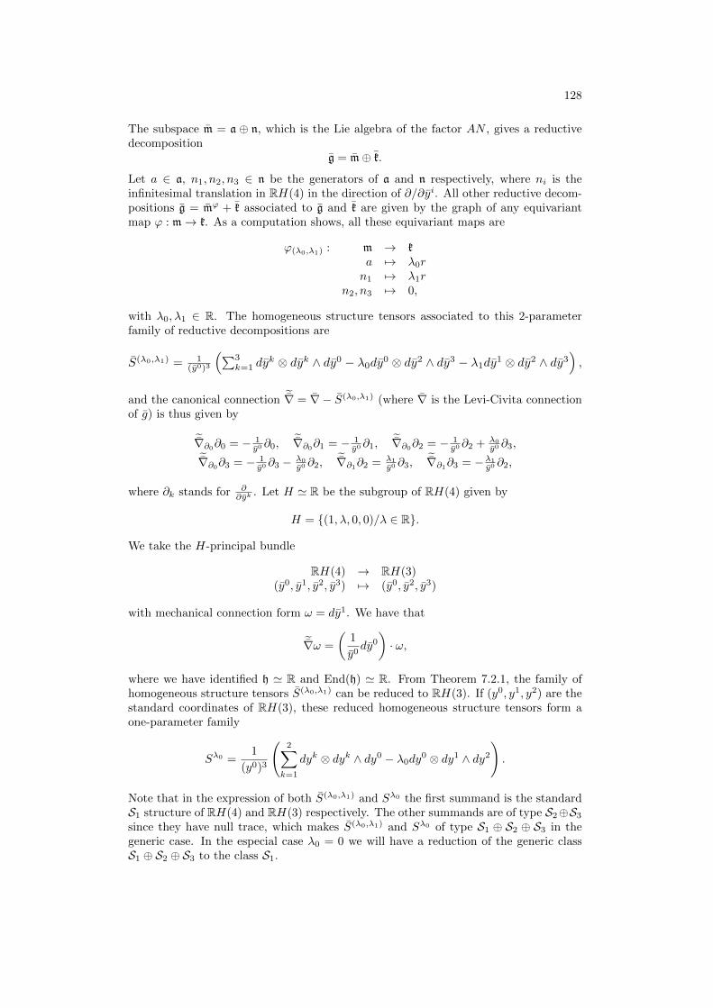
128

The subspace m = a ⊕ n, which is the Lie algebra of the factor AN , gives a reductivedecomposition

g = m⊕ k.

Let a ∈ a, n1, n2, n3 ∈ n be the generators of a and n respectively, where ni is theinfinitesimal translation in RH(4) in the direction of ∂/∂yi. All other reductive decom-positions g = mϕ + k associated to g and k are given by the graph of any equivariantmap ϕ : m→ k. As a computation shows, all these equivariant maps are

ϕ(λ0,λ1) : m → ka 7→ λ0rn1 7→ λ1r

n2, n3 7→ 0,

with λ0, λ1 ∈ R. The homogeneous structure tensors associated to this 2-parameterfamily of reductive decompositions are

S(λ0,λ1) = 1(y0)3

(∑3k=1 dy

k ⊗ dyk ∧ dy0 − λ0dy0 ⊗ dy2 ∧ dy3 − λ1dy

1 ⊗ dy2 ∧ dy3),

and the canonical connection ˜∇ = ∇ − S(λ0,λ1) (where ∇ is the Levi-Civita connectionof g) is thus given by

˜∇∂0∂0 = − 1

y0 ∂0,˜∇∂0

∂1 = − 1y0 ∂1,

˜∇∂0∂2 = − 1

y0 ∂2 + λ0

y0 ∂3,˜∇∂0∂3 = − 1y0 ∂3 − λ0

y0 ∂2,˜∇∂1∂2 = λ1

y0 ∂3,˜∇∂1∂3 = −λ1

y0 ∂2,

where ∂k stands for ∂∂yk

. Let H ' R be the subgroup of RH(4) given by

H = (1, λ, 0, 0)/λ ∈ R.

We take the H-principal bundle

RH(4) → RH(3)(y0, y1, y2, y3) 7→ (y0, y2, y3)

with mechanical connection form ω = dy1. We have that

˜∇ω =

(1

y0dy0

)· ω,

where we have identified h ' R and End(h) ' R. From Theorem 7.2.1, the family ofhomogeneous structure tensors S(λ0,λ1) can be reduced to RH(3). If (y0, y1, y2) are thestandard coordinates of RH(3), these reduced homogeneous structure tensors form aone-parameter family

Sλ0 =1

(y0)3

(2∑k=1

dyk ⊗ dyk ∧ dy0 − λ0dy0 ⊗ dy1 ∧ dy2

).

Note that in the expression of both S(λ0,λ1) and Sλ0 the first summand is the standardS1 structure of RH(4) and RH(3) respectively. The other summands are of type S2⊕S3

since they have null trace, which makes S(λ0,λ1) and Sλ0 of type S1 ⊕ S2 ⊕ S3 in thegeneric case. In the especial case λ0 = 0 we will have a reduction of the generic classS1 ⊕ S2 ⊕ S3 to the class S1.

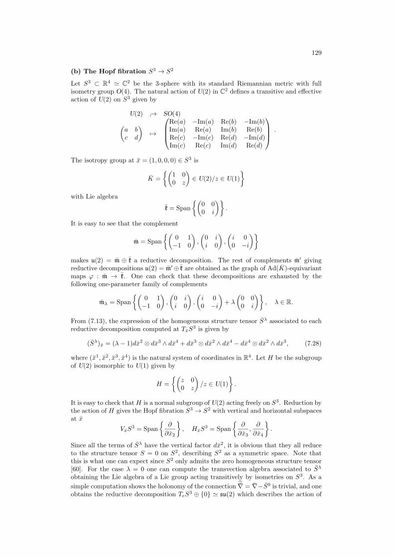
129

(b) The Hopf fibration S3 → S2

Let S3 ⊂ R4 ' C2 be the 3-sphere with its standard Riemannian metric with fullisometry group O(4). The natural action of U(2) in C2 defines a transitive and effectiveaction of U(2) on S3 given by

U(2) → SO(4)(a bc d

)7→

Re(a) −Im(a) Re(b) −Im(b)Im(a) Re(a) Im(b) Re(b)Re(c) −Im(c) Re(d) −Im(d)Im(c) Re(c) Im(d) Re(d)

.

The isotropy group at x = (1, 0, 0, 0) ∈ S3 is

K =

(1 00 z

)∈ U(2)/z ∈ U(1)

with Lie algebra

k = Span

(0 00 i

).

It is easy to see that the complement

m = Span

(0 1−1 0

),

(0 ii 0

),

(i 00 −i

)makes u(2) = m ⊕ k a reductive decomposition. The rest of complements m′ givingreductive decompositions u(2) = m′⊕ k are obtained as the graph of Ad(K)-equivariantmaps ϕ : m → k. One can check that these decompositions are exhausted by thefollowing one-parameter family of complements

mλ = Span

(0 1−1 0

),

(0 ii 0

),

(i 00 −i

)+ λ

(0 00 i

), λ ∈ R.

From (7.13), the expression of the homogeneous structure tensor Sλ associated to eachreductive decomposition computed at TxS

3 is given by

(Sλ)x = (λ− 1)dx2 ⊗ dx3 ∧ dx4 + dx3 ⊗ dx2 ∧ dx4 − dx4 ⊗ dx2 ∧ dx3, (7.28)

where (x1, x2, x3, x4) is the natural system of coordinates in R4. Let H be the subgroupof U(2) isomorphic to U(1) given by

H =

(z 00 z

)/z ∈ U(1)

.

It is easy to check that H is a normal subgroup of U(2) acting freely on S3. Reduction bythe action of H gives the Hopf fibration S3 → S2 with vertical and horizontal subspacesat x

VxS3 = Span

∂

∂x2

, HxS

3 = Span

∂

∂x3,∂

∂x4

.

Since all the terms of Sλ have the vertical factor dx2, it is obvious that they all reduceto the structure tensor S = 0 on S2, describing S2 as a symmetric space. Note thatthis is what one can expect since S2 only admits the zero homogeneous structure tensor[60]. For the case λ = 0 one can compute the transvection algebra associated to Sλ

obtaining the Lie algebra of a Lie group acting transitively by isometries on S3. As a

simple computation shows the holonomy of the connection ˜∇ = ∇−S0 is trivial, and oneobtains the reductive decomposition TeS

3 ⊕ 0 ' su(2) which describes the action of

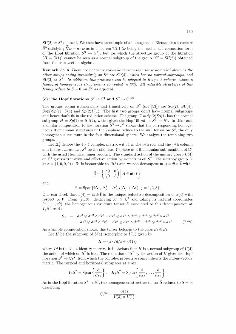
130

SU(2) ' S3 on itself. We then have an example of a homogeneous Riemannian structure

S0 satisfying ˜∇ω = α · ω as in Theorem 7.2.1 (ω being the mechanical connection formof the Hopf fibration S3 → S2), but for which the structure group of the fibration(H = U(1)) cannot be seen as a normal subgroup of the group (G′ = SU(2)) obtainedfrom the transvection algebra.

Remark 7.2.6 There are not more reducible tensors than those described above as theother groups acting transitively on S3 are SO(4), which has no normal subgroups, andSU(2) ' S3. In addition, this procedure can be adapted to Berger 3-spheres, where afamily of homogeneous structures is computed in [32]. All reducible structures of thisfamily reduce to S = 0 on S2 as expected.

(c) The Hopf fibrations S7 → S4 and S7 → CP 3

The groups acting isometrically and transitively on S7 (see [53]) are SO(7), SU(4),Sp(2)Sp(1), U(4) and Sp(2)U(1). The first two groups don’t have normal subgroupsand hence don’t fit in the reduction scheme. The group G = Sp(2)Sp(1) has the normalsubgroup H = Sp(1) = SU(2), which gives the Hopf fibration S7 → S4. In this case,a similar computation to the fibration S3 → S2 shows that the corresponding homoge-neous Riemannian structures in the 7-sphere reduce to the null tensor on S4, the onlyhomogeneous structure in the four dimensional sphere. We analyze the remaining twogroups.

Let ∆ij denote the 4× 4 complex matrix with 1 in the i-th row and the j-th column

and the rest zeros. Let S7 be the standard 7-sphere as a Riemannian sub-manifold of C4

with the usual Hermitian inner product. The standard action of the unitary group U(4)on C4 gives a transitive and effective action by isometries on S7. The isotropy group Kat x = (1, 0, 0, 0) ∈ S7 is isomorphic to U(3) and we can decompose u(4) = m⊕ k with

k =

(0 00 A

) ∣∣∣∣A ∈ u(3)

and

m = Spani∆11, ∆1

j −∆j1, i(∆

1j + ∆j

1), j = 1, 2, 3.One can check that u(4) = m ⊕ k is the unique reductive decomposition of u(4) withrespect to k. From (7.13), identifying R8 ' C4 and taking its natural coordinates(x1, . . . , x8), the homogeneous structure tensor S associated to this decomposition atTxS

7 reads

Sx = dx3 ⊗ dx2 ∧ dx4 − dx4 ⊗ dx2 ∧ dx3 + dx5 ⊗ dx2 ∧ dx6

−dx6 ⊗ dx2 ∧ dx5 + dx7 ⊗ dx2 ∧ dx8 − dx8 ⊗ dx2 ∧ dx7. (7.29)

As a simple computation shows, this tensor belongs to the class S2 ⊕ S3.Let H be the subgroup of U(4) isomorphic to U(1) given by

H = z · Id/z ∈ U(1)

where Id is the 4×4 identity matrix. It is obvious that H is a normal subgroup of U(4)the action of which on S7 is free. The reduction of S7 by the action of H gives the Hopffibration S7 → CP 3 from which the complex projective space inherits the Fubiny-Studymetric. The vertical and horizontal subspaces at x are

VxS7 = Span

∂

∂x2

, HxS

7 = Span

∂

∂x3, . . . ,

∂

∂x8

.

As in the Hopf fibration S3 → S2, the homogeneous structure tensor S reduces to S = 0,describing

CP 3 =U(4)

U(3)×U(1)

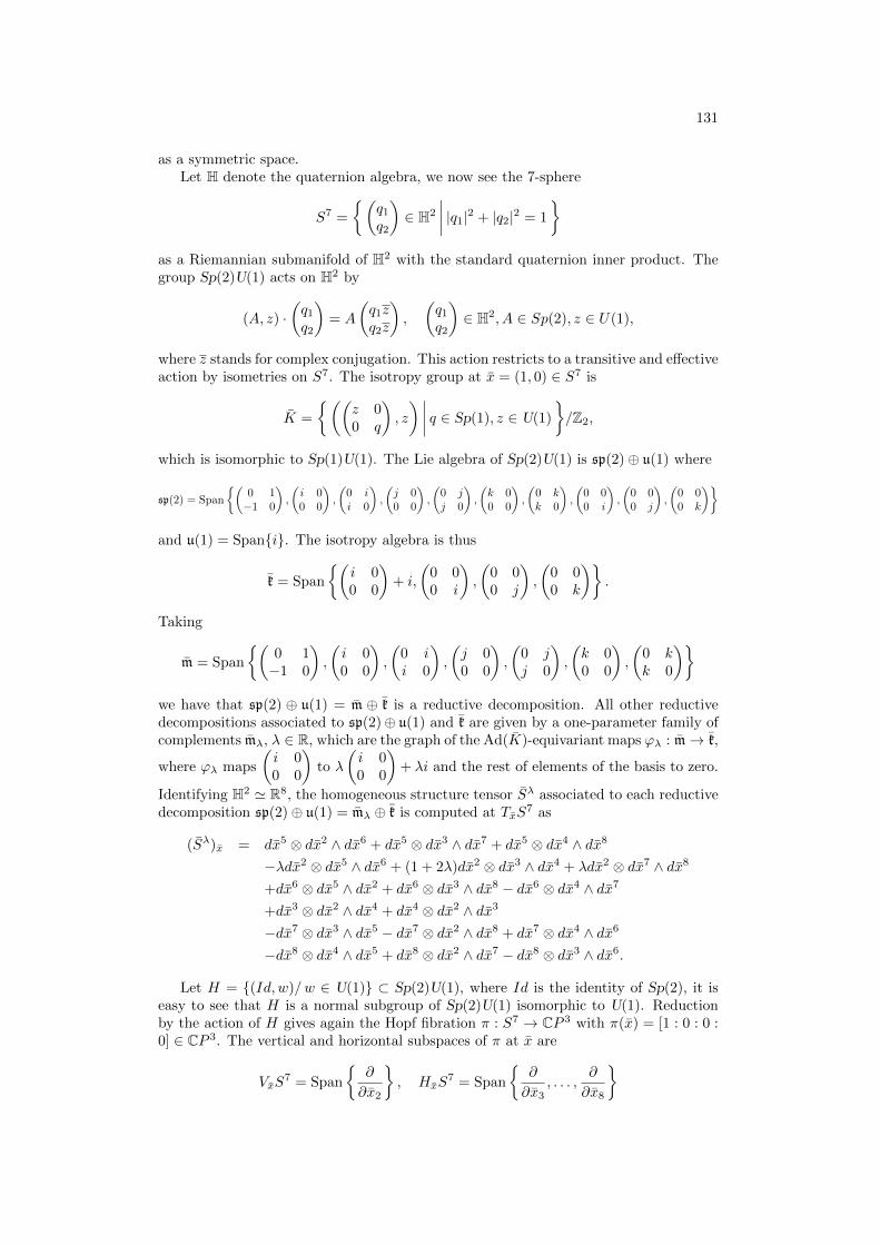
131

as a symmetric space.Let H denote the quaternion algebra, we now see the 7-sphere

S7 =

(q1

q2

)∈ H2

∣∣∣∣ |q1|2 + |q2|2 = 1

as a Riemannian submanifold of H2 with the standard quaternion inner product. Thegroup Sp(2)U(1) acts on H2 by

(A, z) ·(q1

q2

)= A

(q1zq2z

),

(q1

q2

)∈ H2, A ∈ Sp(2), z ∈ U(1),

where z stands for complex conjugation. This action restricts to a transitive and effectiveaction by isometries on S7. The isotropy group at x = (1, 0) ∈ S7 is

K =

((z 00 q

), z

) ∣∣∣∣ q ∈ Sp(1), z ∈ U(1)

/Z2,

which is isomorphic to Sp(1)U(1). The Lie algebra of Sp(2)U(1) is sp(2)⊕ u(1) where

sp(2) = Span

(0 1−1 0

),

(i 00 0

),

(0 ii 0

),

(j 00 0

),

(0 jj 0

),

(k 00 0

),

(0 kk 0

),

(0 00 i

),

(0 00 j

),

(0 00 k

)

and u(1) = Spani. The isotropy algebra is thus

k = Span

(i 00 0

)+ i,

(0 00 i

),

(0 00 j

),

(0 00 k

).

Taking

m = Span

(0 1−1 0

),

(i 00 0

),

(0 ii 0

),

(j 00 0

),

(0 jj 0

),

(k 00 0

),

(0 kk 0

)we have that sp(2) ⊕ u(1) = m ⊕ k is a reductive decomposition. All other reductivedecompositions associated to sp(2)⊕ u(1) and k are given by a one-parameter family ofcomplements mλ, λ ∈ R, which are the graph of the Ad(K)-equivariant maps ϕλ : m→ k,

where ϕλ maps

(i 00 0

)to λ

(i 00 0

)+ λi and the rest of elements of the basis to zero.

Identifying H2 ' R8, the homogeneous structure tensor Sλ associated to each reductivedecomposition sp(2)⊕ u(1) = mλ ⊕ k is computed at TxS

7 as

(Sλ)x = dx5 ⊗ dx2 ∧ dx6 + dx5 ⊗ dx3 ∧ dx7 + dx5 ⊗ dx4 ∧ dx8

−λdx2 ⊗ dx5 ∧ dx6 + (1 + 2λ)dx2 ⊗ dx3 ∧ dx4 + λdx2 ⊗ dx7 ∧ dx8

+dx6 ⊗ dx5 ∧ dx2 + dx6 ⊗ dx3 ∧ dx8 − dx6 ⊗ dx4 ∧ dx7

+dx3 ⊗ dx2 ∧ dx4 + dx4 ⊗ dx2 ∧ dx3

−dx7 ⊗ dx3 ∧ dx5 − dx7 ⊗ dx2 ∧ dx8 + dx7 ⊗ dx4 ∧ dx6

−dx8 ⊗ dx4 ∧ dx5 + dx8 ⊗ dx2 ∧ dx7 − dx8 ⊗ dx3 ∧ dx6.

Let H = (Id, w)/w ∈ U(1) ⊂ Sp(2)U(1), where Id is the identity of Sp(2), it iseasy to see that H is a normal subgroup of Sp(2)U(1) isomorphic to U(1). Reductionby the action of H gives again the Hopf fibration π : S7 → CP 3 with π(x) = [1 : 0 : 0 :0] ∈ CP 3. The vertical and horizontal subspaces of π at x are

VxS7 = Span

∂

∂x2

, HxS

7 = Span

∂

∂x3, . . . ,

∂

∂x8

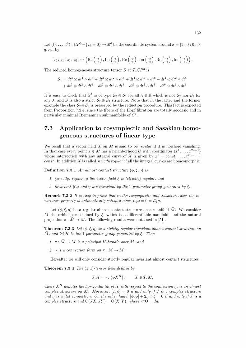
132

Let (t1, . . . , t6) : CP 3−z0 = 0 → R6 be the coordinate system around x = [1 : 0 : 0 : 0]given by

[z0 : z1 : z2 : z3] 7→(

Re(z1z0

), Im

(z1z0

),Re

(z2z0

), Im

(z2z0

),Re

(z3z0

), Im

(z3z0

)).

The reduced homogeneous structure tensor S at TxCP 3 is

Sx = dt3 ⊗ dt1 ∧ dt5 + dt3 ⊗ dt2 ∧ dt6 + dt4 ⊗ dt1 ∧ dt6 − dt4 ⊗ dt2 ∧ dt5

+ dt5 ⊗ dt2 ∧ dt4 − dt5 ⊗ dt1 ∧ dt3 − dt6 ⊗ dt2 ∧ dt3 − dt6 ⊗ dt1 ∧ dt4.

It is easy to check that Sλ is of type S2 ⊕ S3 for all λ ∈ R which is not S2 nor S3 forany λ, and S is also a strict S2 ⊕ S3 structure. Note that in the latter and the formerexample the class S2⊕S3 is preserved by the reduction procedure. This fact is expectedfrom Proposition 7.2.4, since the fibers of the Hopf fibration are totally geodesic and inparticular minimal Riemannian submanifolds of S7.

7.3 Application to cosymplectic and Sasakian homo-geneous structures of linear type

We recall that a vector field X on M is said to be regular if it is nowhere vanishing.In that case every point x ∈ M has a neighborhood U with coordinates (x1, . . . , x2n+1)whose intersection with any integral curve of X is given by x1 = const., . . . , x2n+1 =const. In addition X is called strictly regular if all the integral curves are homeomorphic.

Definition 7.3.1 An almost contact structure (φ, ξ, η) is

1. (strictly) regular if the vector field ξ is (strictly) regular, and

2. invariant if φ and η are invariant by the 1-parameter group generated by ξ.

Remark 7.3.2 It is easy to prove that in the cosymplectic and Sasakian cases the in-variance property is automatically satisfied since Lξφ = 0 = Lξη.

Let (φ, ξ, η) be a regular almost contact structure on a manifold M . We considerM the orbit space defined by ξ, which is a differentiable manifold, and the naturalprojection π : M →M . The following results were obtained in [51].

Theorem 7.3.3 Let (φ, ξ, η) be a strictly regular invariant almost contact structure onM , and let H be the 1-parameter group generated by ξ. Then

1. π : M →M is a principal H-bundle over M , and

2. η is a connection form on π : M →M .

Hereafter we will only consider strictly regular invariant almost contact structures.

Theorem 7.3.4 The (1, 1)-tensor field defined by

JxX = π∗(φXH

), X ∈ TxM,

where XH denotes the horizontal lift of X with respect to the connection η, is an almostcomplex structure on M . Moreover, [φ, φ] = 0 if and only if J is a complex structureand η is a flat connection. On the other hand, [φ, φ] + 2η ⊗ ξ = 0 if and only if J is acomplex structure and Θ(JX, JY ) = Θ(X,Y ), where π∗Θ = dη.

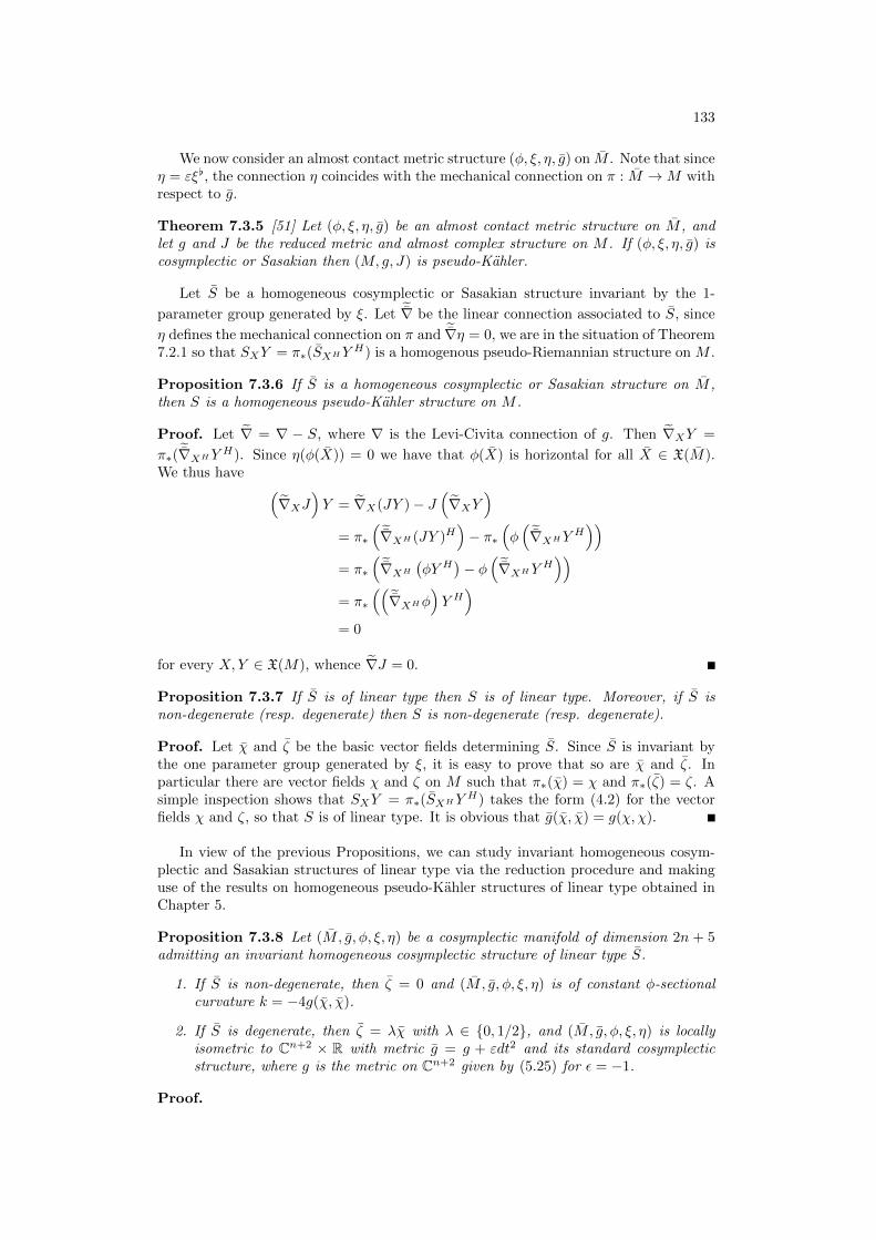
133

We now consider an almost contact metric structure (φ, ξ, η, g) on M . Note that sinceη = εξ[, the connection η coincides with the mechanical connection on π : M →M withrespect to g.

Theorem 7.3.5 [51] Let (φ, ξ, η, g) be an almost contact metric structure on M , andlet g and J be the reduced metric and almost complex structure on M . If (φ, ξ, η, g) iscosymplectic or Sasakian then (M, g, J) is pseudo-Kahler.

Let S be a homogeneous cosymplectic or Sasakian structure invariant by the 1-

parameter group generated by ξ. Let ˜∇ be the linear connection associated to S, since

η defines the mechanical connection on π and ˜∇η = 0, we are in the situation of Theorem7.2.1 so that SXY = π∗(SXHY

H) is a homogenous pseudo-Riemannian structure on M .

Proposition 7.3.6 If S is a homogeneous cosymplectic or Sasakian structure on M ,then S is a homogeneous pseudo-Kahler structure on M .

Proof. Let ∇ = ∇ − S, where ∇ is the Levi-Civita connection of g. Then ∇XY =

π∗(˜∇XHY H). Since η(φ(X)) = 0 we have that φ(X) is horizontal for all X ∈ X(M).

We thus have (∇XJ

)Y = ∇X(JY )− J

(∇XY

)= π∗

( ˜∇XH (JY )H)− π∗

(φ( ˜∇XHY H))

= π∗

( ˜∇XH (φY H)− φ( ˜∇XHY H))= π∗

(( ˜∇XHφ)Y H)= 0

for every X,Y ∈ X(M), whence ∇J = 0.

Proposition 7.3.7 If S is of linear type then S is of linear type. Moreover, if S isnon-degenerate (resp. degenerate) then S is non-degenerate (resp. degenerate).

Proof. Let χ and ζ be the basic vector fields determining S. Since S is invariant bythe one parameter group generated by ξ, it is easy to prove that so are χ and ζ. Inparticular there are vector fields χ and ζ on M such that π∗(χ) = χ and π∗(ζ) = ζ. Asimple inspection shows that SXY = π∗(SXHY

H) takes the form (4.2) for the vectorfields χ and ζ, so that S is of linear type. It is obvious that g(χ, χ) = g(χ, χ).

In view of the previous Propositions, we can study invariant homogeneous cosym-plectic and Sasakian structures of linear type via the reduction procedure and makinguse of the results on homogeneous pseudo-Kahler structures of linear type obtained inChapter 5.

Proposition 7.3.8 Let (M, g, φ, ξ, η) be a cosymplectic manifold of dimension 2n + 5admitting an invariant homogeneous cosymplectic structure of linear type S.

1. If S is non-degenerate, then ζ = 0 and (M, g, φ, ξ, η) is of constant φ-sectionalcurvature k = −4g(χ, χ).

2. If S is degenerate, then ζ = λχ with λ ∈ 0, 1/2, and (M, g, φ, ξ, η) is locallyisometric to Cn+2 × R with metric g = g + εdt2 and its standard cosymplecticstructure, where g is the metric on Cn+2 given by (5.25) for ε = −1.

Proof.

134

1. Since the reduced homogeneous structure S is a non-degenerate homogeneouspseudo-Kahler structure of linear type, we have by Proposition 5.1.2 that (M, g, J)has constant holomorphic sectional curvature c = −4g(π∗χ, π∗χ). Let X be avector in the contact distribution, by O’Neill’s formulas for pseudo-Riemanniansubmersions

K(X, φX

)= K

(π∗X, π∗φX

)+

3

4

([X, φX]V

)2,

where K and K denote sectional curvatures on M and M respectively, and Xis unitary. As (M, g, φ, ξ, η) is cosymplectic, the curvature of the connection ηvanishes so that [X, φX]V = 0. We thus conclude that

K(X, φX

)= K

(π∗X, π∗φX

)= K

(π∗X, Jπ∗X

)= −4g(π∗χ, π∗χ) = −4g(χ, χ).

Note that g(χ, χ) is constant since ˜∇g = 0, and ˜∇S = 0 implies ˜∇χ = 0, where ˜∇is the ASK-connection associated to S.

2. Since S is a degenerate homogeneous pseudo-Kahler structure of linear type deter-mined by the vector fields π∗χ and π∗ζ, we have by Corollary 5.2.3 that π∗ζ = λπ∗χwith λ ∈ 0, 1/2. This implies ζ = λχ, as ζ and χ are basic by definition.

Let now H be the one parameter group generated by ξ. Since (M, g, φ, ξ, η) iscosymplectic, the curvature of the connection η on π : M → M vanishes. Thisimplies that for every p ∈ M we can choose a trivialization Ψ : π−1(U)→ U ×Hwith Ψ(p) = (π(p), e) such that Ψ∗(HqM) = Tπ(p)U+0 for all q ∈ π−1(U), wheree is the neutral element of H and HqM is the horizontal subspace at q with respectto η, which coincides with the contact distribution Spanξ⊥. Taking a coordinatet ∈ (−δ, δ) on a neighborhood of H around e, we obtain a diffeomorphism Ψ : V →U×(−δ, δ), where V is a certain neighborhood around p. By construction we havethat (Ψ−1)∗(g) = gU + εdt2, where gU is the reduced metric g on M restricted toU . Reducing U if necessary we have that gU is holomorphically isometric to anopen set W of Cn+2 with metric (5.25) for ε = −1. Finally, it is easy to see thatthe cosymplectic structure on M transforms by Ψ into the standard cosymplecticstructure of Cn+2 × R restricted to the open set W × (−δ, δ).

Corollary 7.3.9 Let (M, g, φ, ξ, η) be a cosymplectic manifold of dimension 2n + 5admitting an invariant degenerate homogeneous cosymplectic structure of linear type.Then g is Ricci-flat and the holonomy algebra is given by the one dimensional Liealgebra

hol(g) ∼= R

i i 0−i −i 00 0 0n

+ 0 ⊂ su(1, 1) + 0 ⊂ Lie(U(p, q)× 1),

with p+ q = n+ 2.

Proof. This result follows immediately from the fact that g is Ricci-flat and has holon-omy algebra

hol(g) ∼= R

i i 0−i −i 00 0 0n

.

135

Proposition 7.3.10 Let (M, g, φ, ξ, η) be a Sasakian manifold admitting an invarianthomogeneous Sasakian structure of linear type S.

1. If S is non-degenerate, then ζ = 0 and (M, g, φ, ξ, η) is of constant φ-sectionalcurvature k = −4g(χ, χ) + 3.

2. If S is degenerate, then ζ = λχ with λ ∈ 0, 1/2, and there is a set of coordinatesz1, z2, w1, w2, xa, ya, t such that the metric takes the form

g = g + εηdt,

where g is given by (5.25) for ε = −1.

Proof.

1. Since the reduced homogeneous structure S is a non-degenerate homogeneouspseudo-Kahler structure of linear type, we have by Proposition 5.1.2 that (M, g, J)has constant holomorphic sectional curvature c = −4g(π∗χ, π∗χ). Let X be avector in the contact distribution, by O’Neill’s formulas for pseudo-Riemanniansubmersions

K(X, φX

)= K

(π∗X, π∗φX

)+

3

4

([X, φX]V

)2,

where K and K denote sectional curvatures on M and M respectively, and X isunitary. As (M, g, φ, ξ, η) is Sasakian, the curvature form of the connection η isgiven by dη = Φ, so that

[X, φX]V = 2dη(X, φX) = 2Φ(X, φX).

We thus conclude that

K(X, φX

)= K

(π∗X, Jπ∗X

)+ 3Φ(X, φX)2

= −4g(π∗χ, π∗χ) + 3 = −4g(χ, χ) + 3.

Note that by the same reason as before g(χ, χ) is constant.

2. Since S is a degenerate homogeneous pseudo-Kahler structure of linear type deter-mined by the vector fields π∗χ and π∗ζ, we have by Corollary 5.2.3 that π∗ζ = λπ∗χwith λ ∈ 0, 1/2, so that ζ = λχ. Let now H be the 1-parameter group generatedby ξ. Let p ∈ M we consider a trivialization of the principal bundle π : M →M ,i.e., we consider a diffeomorphism Ψ : π−1(U) → U ×H, where Ψ(p) = (π(p), e)

and e is the neutral element of H. Let ξ = Ψ∗,p(ξp) ∈ h, there is an open interval

(−δ, δ) such that f : (−δ, δ) → H given by f(t) = exp(tξ) is a diffeomorphismonto its image. We thus consider the map

F : U × (−δ, δ) id×f→ U ×H Ψ−1

→ π−1(U),

which is a diffeomorphism onto a certain neighborhood of p. Then, the pullback ofthe metric g by F is F ∗g = gU+εF ∗ηdt, where gU is the reduced metric g restrictedto U . Reducing U if necessary we can take coordinates z1, z2, w1, w2, xa, ya onU such that gU is expressed as (5.25) for ε = −1. We have thus constructedcoordinates z1, z2, w1, w2, xa, ya, t around p with respect to which g = g + εηdtwith g given by (5.25) for ε = −1.

Note that due to the non-integrability of the contact distribution, in the previousproof Ψ∗(HqM) 6= Tπ(p)U + 0 for general q ∈ π−1(U). This means that F ∗η 6= dt,

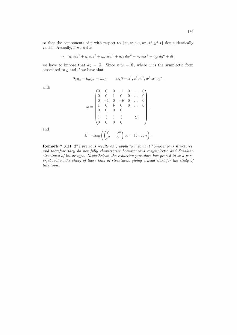
136

so that the components of η with respect to z1, z2, w1, w2, xa, ya, t don’t identicallyvanish. Actually, if we write

η = ηz1dz1 + ηz2dz2 + ηw1dw1 + ηw2dw2 + ηxadxa + ηyady

a + dt,

we have to impose that dη = Φ. Since π∗ω = Φ, where ω is the symplectic formassociated to g and J we have that

∂βηα − ∂αηα = ωαβ , α, β = z1, z2, w1, w2, xa, ya,

with

ω =

0 0 0 −1 0 . . . 00 0 1 0 0 . . . 00 −1 0 −b 0 . . . 01 0 b 0 0 . . . 00 0 0 0...

......

... Σ0 0 0 0

,

and

Σ = diag

((0 −εaεa 0

), a = 1, . . . , n

).

Remark 7.3.11 The previous results only apply to invariant homogeneous structures,and therefore they do not fully characterize homogeneous cosymplectic and Sasakianstructures of linear type. Nevertheless, the reduction procedure has proved to be a pow-erful tool in the study of these kind of structures, giving a head start for the study ofthis topic.

Chapter 8

Appendix: Computationsconcerning formula (5.17)

We start with formulaRξU = −2aεfθ(JU)θ ∧ (θ J), (8.1)

and apply

(∇XR)Y ZWU = −RSXY ZWU −RY SXZWU −RY ZSXWU −RY ZWSXU ,

that is,

(∇XR)Y ZWU = −g(X,Y )RξZWU + g(ξ, Y )RXZWU − εg(X, JY )RJξZWU

+ εg(ξ, JY )RJXZWU − g(X,Z)RY ξWU + g(ξ, Z)RY XWU

− εg(X, JZ)RY JξWU + εg(ξ, JZ)RY JXWU − g(X,W )RY ZξU

+ g(ξ,W )RY ZXU − εg(X, JW )RY ZJξU + εg(ξ, JW )RY ZJXU

− g(X,U)RY ZWξ + g(ξ, U)RY ZWX − εg(X, JU)RY ZWJξ

+ εg(ξ, JU)RY ZWJX .

This gives

SXYZ

(∇XR)Y ZWU = −g(X,Y )RξZWU + g(ξ, Y )RXZWU − εg(X, JY )RJξZWU

+ εg(ξ, JY )RJXZWU − g(X,Z)RY ξWU + g(ξ, Z)RY XWU

− εg(X, JZ)RY JξWU + εg(ξ, JZ)RY JXWU − g(X,W )RY ZξU

+ g(ξ,W )RY ZXU − εg(X, JW )RY ZJξU + εg(ξ, JW )RY ZJXU

− g(X,U)RY ZWξ + g(ξ, U)RY ZWX − εg(X, JU)RY ZWJξ

+ εg(ξ, JU)RY ZWJX − g(Y,Z)RξXWU + g(ξ, Z)RY XWU

− εg(Y, JZ)RJξXWU + εg(ξ, JZ)RJY XWU − g(Y,X)RZξWU

+ g(ξ,X)RZYWU − εg(Y, JX)RZJξWU + εg(ξ, JX)RZJYWU

− g(Y,W )RZXξU + g(ξ,W )RZXY U − εg(Y, JW )RZXJξU

+ εg(ξ, JW )RZXJY U − g(Y,U)RZXWξ + g(ξ, U)RZXWY

− εg(Y, JU)RZXWJξ + εg(ξ, JU)RZXWJY − g(Z,X)RξYWU

+ g(ξ,X)RZYWU − εg(Z, JX)RJξYWU + εg(ξ, JX)RJZYWU

− g(Z, Y )RXξWU + g(ξ, Y )RXZWU − εg(Z, JY )RXJξWU

+ εg(ξ, JY )RXJZWU − g(Z,W )RXY ξU + g(ξ,W )RXY ZU

− εg(Z, JW )RXY JξU + εg(ξ, JW )RXY JZU − g(Z,U)RXYWξ

+ g(ξ, U)RXYWZ − εg(Z, JU)RXYWJξ + εg(ξ, JU)RXYWJZ .

137

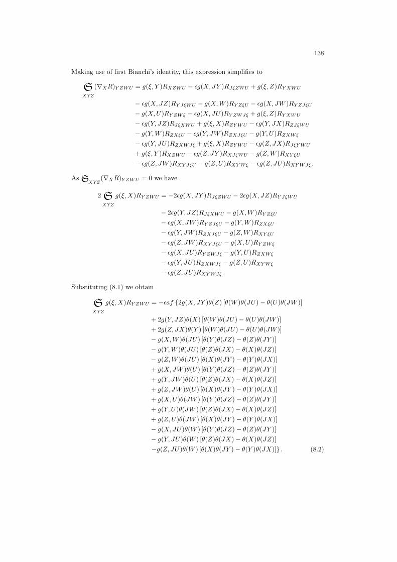
138

Making use of first Bianchi’s identity, this expression simplifies to

SXYZ

(∇XR)Y ZWU = g(ξ, Y )RXZWU − εg(X, JY )RJξZWU + g(ξ, Z)RY XWU

− εg(X,JZ)RY JξWU − g(X,W )RY ZξU − εg(X, JW )RY ZJξU

− g(X,U)RY ZWξ − εg(X, JU)RY ZWJξ + g(ξ, Z)RY XWU

− εg(Y, JZ)RJξXWU + g(ξ,X)RZYWU − εg(Y, JX)RZJξWU

− g(Y,W )RZXξU − εg(Y, JW )RZXJξU − g(Y,U)RZXWξ

− εg(Y, JU)RZXWJξ + g(ξ,X)RZYWU − εg(Z, JX)RJξYWU

+ g(ξ, Y )RXZWU − εg(Z, JY )RXJξWU − g(Z,W )RXY ξU

− εg(Z, JW )RXY JξU − g(Z,U)RXYWξ − εg(Z, JU)RXYWJξ.

As SXYZ(∇XR)Y ZWU = 0 we have

2 SXYZ

g(ξ,X)RY ZWU = −2εg(X, JY )RJξZWU − 2εg(X,JZ)RY JξWU

− 2εg(Y, JZ)RJξXWU − g(X,W )RY ZξU

− εg(X, JW )RY ZJξU − g(Y,W )RZXξU

− εg(Y, JW )RZXJξU − g(Z,W )RXY ξU

− εg(Z, JW )RXY JξU − g(X,U)RY ZWξ

− εg(X, JU)RY ZWJξ − g(Y,U)RZXWξ

− εg(Y, JU)RZXWJξ − g(Z,U)RXYWξ

− εg(Z, JU)RXYWJξ.

Substituting (8.1) we obtain

SXYZ

g(ξ,X)RY ZWU = −εaf 2g(X, JY )θ(Z) [θ(W )θ(JU)− θ(U)θ(JW )]

+ 2g(Y, JZ)θ(X) [θ(W )θ(JU)− θ(U)θ(JW )]

+ 2g(Z, JX)θ(Y ) [θ(W )θ(JU)− θ(U)θ(JW )]

− g(X,W )θ(JU) [θ(Y )θ(JZ)− θ(Z)θ(JY )]

− g(Y,W )θ(JU) [θ(Z)θ(JX)− θ(X)θ(JZ)]

− g(Z,W )θ(JU) [θ(X)θ(JY )− θ(Y )θ(JX)]

+ g(X,JW )θ(U) [θ(Y )θ(JZ)− θ(Z)θ(JY )]

+ g(Y, JW )θ(U) [θ(Z)θ(JX)− θ(X)θ(JZ)]

+ g(Z, JW )θ(U) [θ(X)θ(JY )− θ(Y )θ(JX)]

+ g(X,U)θ(JW ) [θ(Y )θ(JZ)− θ(Z)θ(JY )]

+ g(Y, U)θ(JW ) [θ(Z)θ(JX)− θ(X)θ(JZ)]

+ g(Z,U)θ(JW ) [θ(X)θ(JY )− θ(Y )θ(JX)]

− g(X,JU)θ(W ) [θ(Y )θ(JZ)− θ(Z)θ(JY )]

− g(Y, JU)θ(W ) [θ(Z)θ(JX)− θ(X)θ(JZ)]

−g(Z, JU)θ(W ) [θ(X)θ(JY )− θ(Y )θ(JX)] . (8.2)

139

Switching Y and W , and Z and U , the previous formula becomes

SXYZ

g(ξ,X)RWUY Z = −εaf 2g(X, JW )θ(U) [θ(Y )θ(JZ)− θ(Z)θ(JY )]

+ 2g(W,JU)θ(X) [θ(Y )θ(JZ)− θ(Z)θ(JY )]

+ 2g(U, JX)θ(W ) [θ(Y )θ(JZ)− θ(Z)θ(JY )]

− g(X,Y )θ(JZ) [θ(W )θ(JU)− θ(U)θ(JW )]

− g(Y,W )θ(JZ) [θ(U)θ(JX)− θ(X)θ(JU)]

− g(U, Y )θ(JZ) [θ(X)θ(JW )− θ(W )θ(JX)]

+ g(X, JY )θ(Z) [θ(W )θ(JU)− θ(U)θ(JW )]

+ g(W,JY )θ(Z) [θ(U)θ(JX)− θ(X)θ(JU)]

+ g(U, JY )θ(Z) [θ(X)θ(JW )− θ(W )θ(JX)]

+ g(X,Z)θ(JY ) [θ(W )θ(JU)− θ(U)θ(JW )]

+ g(W,Z)θ(JY ) [θ(U)θ(JX)− θ(X)θ(JU)]

+ g(Z,U)θ(JY ) [θ(X)θ(JW )− θ(W )θ(JX)]

− g(X,JZ)θ(Y ) [θ(W )θ(JU)− θ(U)θ(JW )]

− g(W,JZ)θ(Y ) [θ(U)θ(JX)− θ(X)θ(JU)]

−g(U, JZ)θ(Y ) [θ(X)θ(JW − θ(W )θ(JX)] . (8.3)

We thus have

(∇XR)Y ZWU = 2aεfg(X,Y )θ(JZ) [θ(W )θ(JU)− θ(W )θ(JU)]

− 2aεfg(X, JY )θ(Z) [θ(W )θ(JU)− θ(W )θ(JU)]

− 2aεfg(X,Z)θ(JY ) [θ(W )θ(JU)− θ(W )θ(JU)]

+ 2aεfg(X, JZ)θ(Y ) [θ(W )θ(JU)− θ(W )θ(JU)]

+ 2aεfg(X,W )θ(JU) [θ(Y )θ(JZ)− θ(Z)θ(JY )]

− 2aεfg(X, JW )θ(U) [θ(Y )θ(JZ)− θ(Z)θ(JY )]

− 2aεfg(X,U)θ(JW ) [θ(Y )θ(JZ)− θ(Z)θ(JY )]

+ 2aεfg(X, JU)θ(W ) [θ(Y )θ(JZ)− θ(Z)θ(JY )]

+ g(ξ, Y )RXZWU + εg(ξ, JY )RJXZWU + g(ξ, Z)RY XWU

+ εg(ξ, JZ)RY JXWU + g(ξ,W )RY ZXU + εg(ξ, JW )RY ZJXU

+ g(ξ, U)RY ZWX + εg(ξ, JU)RY ZWJX ,

and making use of (8.2) and (8.3) we obtain

(∇XR)Y ZWU = −aεf −2g(X,Y )θ(JZ) [θ(W )θ(JU)− θ(JW )θ(U)]

+ 2g(X,JY )θ(Z) [θ(W )θ(JU)− θ(JW )θ(U)]

+ 2g(X,Z)θ(JY ) [θ(W )θ(JU)− θ(JW )θ(U)]

− 2g(X,JZ)θ(Y ) [θ(W )θ(JU)− θ(JW )θ(U)]

− 2g(X,W )θ(JU) [θ(Y )θ(JZ)− θ(Z)θ(JY )]

+ 2g(X,JW )θ(U) [θ(Y )θ(JZ)− θ(Z)θ(JY )]

+ 2g(X,U)θ(JW ) [θ(Y )θ(JZ)− θ(Z)θ(JY )]

−2g(X, JU)θ(W ) [θ(Y )θ(JZ)− θ(Z)θ(JY )]

140

− g(ξ,X)RZYWU

− aεf −2g(X, JY )θ(Z) [θ(W )θ(JU)− θ(U)θ(JW )]

− 2g(Y, JZ)θ(X) [θ(W )θ(JU)− θ(U)θ(JW )]

− 2g(Z, JX)θ(Y ) [θ(W )θ(JU)− θ(U)θ(JW )]

+ g(X,W )θ(JU) [θ(Y )θ(JZ)− θ(Z)θ(JY )]

+ g(Y,W )θ(JU) [θ(Z)θ(JX)− θ(X)θ(JZ)]

+ g(Z,W )θ(JU) [θ(X)θ(JY )− θ(Y )θ(JX)]

− g(X, JW )θ(U) [θ(Y )θ(JZ)− θ(Z)θ(JY )]

− g(Y, JW )θ(U) [θ(Z)θ(JX)− θ(X)θ(JZ)]

− g(Z, JW )θ(U) [θ(X)θ(JY )− θ(Y )θ(JX)]

− g(X,U)θ(JW ) [θ(Y )θ(JZ)− θ(Z)θ(JY )]

− g(Y,U)θ(JW ) [θ(Z)θ(JX)− θ(X)θ(JZ)]

− g(Z,U)θ(JW ) [θ(X)θ(JY )− θ(Y )θ(JX)]

+ g(X, JU)θ(W ) [θ(Y )θ(JZ)− θ(Z)θ(JY )]

+ g(Y, JU)θ(W ) [θ(Z)θ(JX)− θ(X)θ(JZ)]

+g(Z, JU)θ(W ) [θ(X)θ(JY )− θ(Y )θ(JX)]− g(ξ,X)RZYWU

− aεf 2g(X,Y )θ(JZ) [θ(W )θ(JU)− θ(U)θ(JW )]

− 2g(Y, JZ)θ(X) [θ(W )θ(JU)− θ(U)θ(JW )]

− 2g(Z,X)θ(JY ) [θ(W )θ(JU)− θ(U)θ(JW )]

+ g(X,W )θ(JU) [θ(Y )θ(JZ)− θ(Z)θ(JY )]

+ g(JY,W )θ(JU) [θ(JZ)θ(JX) + θ(X)θ(Z)]

+ g(JZ,W )θ(JU) [−θ(X)θ(Y )− θ(JY )θ(JX)]

− g(X, JW )θ(U) [θ(Y )θ(JZ)− θ(Z)θ(JY )]

− g(Y,W )θ(U) [θ(JZ)θ(JX) + θ(X)θ(Z)]

− g(Z,W )θ(U) [−θ(X)θ(Y )− θ(JY )θ(JX)]

− g(X,U)θ(JW ) [θ(Y )θ(JZ)− θ(Z)θ(JY )]

− g(JY, U)θ(JW ) [θ(JZ)θ(JX) + θ(X)θ(Z)]

− g(JZ,U)θ(JW ) [−θ(X)θ(Y )− θ(JY )θ(JX)]

+ g(X, JU)θ(W ) [θ(Y )θ(JZ)− θ(Z)θ(JY )]

+ g(Y,U)θ(W ) [θ(JZ)θ(JX) + θ(X)θ(Z)]

+g(Z,U)θ(W ) [−θ(X)θ(Y )− θ(JY )θ(JX)]− g(ξ,X)RUWY Z

− aεf −2g(X, JW )θ(U) [θ(Y )θ(JZ)− θ(Z)θ(JY )]

− 2g(W,JU)θ(X) [θ(Y )θ(JZ)− θ(Z)θ(JY )]

− 2g(U, JX)θ(W ) [θ(Y )θ(JZ)− θ(Z)θ(JY )]

+ g(X,Y )θ(JZ) [θ(W )θ(JU)− θ(U)θ(JW )]

+ g(Y,W )θ(JZ) [θ(U)θ(JX)− θ(X)θ(JU)]

+ g(U, Y )θ(JZ) [θ(X)θ(JW )− θ(W )θ(JX)]

− g(X, JY )θ(Z) [θ(W )θ(JU)− θ(U)θ(JW )]

− g(W,JY )θ(Z) [θ(U)θ(JX)− θ(X)θ(JU)]

− g(U, JY )θ(Z) [θ(X)θ(JW )− θ(W )θ(JX)]

− g(X,Z)θ(JY ) [θ(W )θ(JU)− θ(U)θ(JW )]

− g(W,Z)θ(JY ) [θ(U)θ(JX)− θ(X)θ(JU)]

141

− g(Z,U)θ(JY ) [θ(X)θ(JW )− θ(W )θ(JX)]

+ g(X, JZ)θ(Y ) [θ(W )θ(JU)− θ(U)θ(JW )]

+ g(W,JZ)θ(Y ) [θ(U)θ(JX)− θ(X)θ(JU)]

+g(U, JZ)θ(Y ) [θ(X)θ(JW − θ(W )θ(JX)]− g(ξ,X)RUWY Z

− aεf 2g(X,W )θ(JU) [θ(Y )θ(JZ)− θ(Z)θ(JY )]

− 2g(W,JU)θ(X) [θ(Y )θ(JZ)− θ(Z)θ(JY )]

− 2g(U,X)θ(JW ) [θ(Y )θ(JZ)− θ(Z)θ(JY )]

+ g(X,Y )θ(JZ) [θ(W )θ(JU)− θ(U)θ(JW )]

+ g(Y, JW )θ(JZ) [θ(JU)θ(JX) + θ(X)θ(U)]

+ g(JU, Y )θ(JZ) [−θ(X)θ(W )− θ(JW )θ(JX)]

− g(X, JY )θ(Z) [θ(W )θ(JU)− θ(U)θ(JW )]

− g(W,Y )θ(Z) [θ(JU)θ(JX) + θ(X)θ(U)]

− g(U, Y )θ(Z) [−θ(X)θ(W )− θ(JW )θ(JX)]

− g(X,Z)θ(JY ) [θ(W )θ(JU)− θ(U)θ(JW )]

− g(JW,Z)θ(JY ) [θ(JU)θ(JX) + θ(X)θ(U)]

− g(Z, JU)θ(JY ) [−θ(X)θ(W )− θ(JW )θ(JX)]

+ g(X, JZ)θ(Y ) [θ(W )θ(JU)− θ(U)θ(JW )]

+ g(W,Z)θ(Y ) [θ(JU)θ(JX) + θ(X)θ(U)]

+ g(U,Z)θ(Y ) [−θ(X)θ(W )− θ(JW )θ(JX)] .

Rearranging the terms the previous formula becomes

(∇XR)Y ZWU = 4g(ξ,X)RY ZWU

− 2aεfθ(X) −g(Y,W ) [θ(U)θ(Z) + θ(JU)θ(JZ)]

+ g(Y,U)[θ(JW )θ(JZ) + θ(W )θ(Z)]

+ g(Z,W ) [θ(U)θ(Y ) + θ(JU)θ(JY )]

− g(Z,U)[θ(JW )θ(JY ) + θ(W )θ(Y )]

+ g(Y, JW ) [θ(U)θ(JZ)− θ(JU)θ(Z)]

− g(Y, JU)[θ(W )θ(JZ)− θ(JW )θ(Z)]

− g(Z, JW ) [θ(U)θ(JY )− θ(JU)θ(Y )]

+ g(Z, JU)[θ(W )θ(JY )− θ(JW )θ(Y )]

− 2g(Y, JZ) [θ(W )θ(JU)− θ(U)θ(JW )]

−2g(W,JU)θ(X) [θ(Y )θ(JZ)− θ(Z)θ(JY )]− aεf 2g(X,Y )θ(JZ) [θ(W )θ(JU)− θ(U)θ(JW )]

− 2g(X,Z)θ(JY ) [θ(W )θ(JU)− θ(U)θ(JW )]

+ 2g(X,W )θ(JU) [θ(Y )θ(JZ)− θ(Z)θ(JY )]

− 2g(X,U)θ(JW ) [θ(Y )θ(JZ)− θ(Z)θ(JY )]

− 2g(X,JY )θ(Z) [θ(W )θ(JU)− θ(U)θ(JW )]

+ 2g(X,JZ)θ(Y ) [θ(W )θ(JU)− θ(U)θ(JW )]

− 2g(X, JW )θ(U) [θ(Y )θ(JZ)− θ(Z)θ(JY )]

+2g(X, JU)θ(W ) [θ(Y )θ(JZ)− θ(Z)θ(JY )] ,

that is,

∇XR = 4θ(X)⊗ (R− 1

2ag r)− 2aε

((X[ ∧ (θ J)) ρ+ (JX[ ∧ (θ)) ρ

),

142

where ρ is the Ricci form and stands for the ε-complex Kulkarni-Nomizu productdefined as

h k(X1, X2, X3, X4) = h(X1, X3)k(X2, X4) + h(X2, X4)k(X1, X3)

− h(X1, X4)k(X2, X3)− h(X2, X3)k(X1, X4)

− εh(X1, JX3)k(X2, JX4)− εh(X2, JX4)k(X1, JX3)

+ εh(X1, JX4)k(X2, JX3) + εh(X2, JX3)k(X1, JX4)

− 2εh(X1, JX2)k(X3, JX4)− 2εh(X3, JX4)k(X1, JX2),

for h and k symmetric (0, 2)-tensors.

Bibliography

[1] E. Abbena, S. Garbiero, Almost hermitian homogeneous structures, Proc. Edinb.Math. Soc. 31 (2) (1988), 375–395.

[2] D.V. Alekseevsky, V. Cortes, Classification of pseudo-Riemannian symmetricspaces of quaternionic Kahler type, Lie Groups and Invariant Theory, Amer. Math.Soc. Transl. (2) 213, Amer. Math. Soc., Providence, RI., 2005, 33–62.

[3] D.V. Alekseevsky, C. Medori, A. Tomassini, Homogeneous para-Kahler Einsteinmanifolds, arXiv:0806.2272v2.

[4] W. Ambrose, I.M. Singer, On homogeneous Riemannian manifolds, Duke Math. J.25 (1958), 647–669.

[5] H. Bacry, Lecons sur la theorie des groupes et les symetries des particleselementaires, Gordon and Breach, Paris, 1967.

[6] M. Barros, A. Romero, Indefinite Kahler Manifolds, Math. Ann. 261 (1982), 55–62.

[7] A.O. Barut, R. Raczka, Theory of group Representations and Applications, PolishScientific Publishers, Warszawa (1977).

[8] W. Batat, P.M. Gadea, J.A. Oubina, Homogeneous pseudo-Riemannian structuresof linear type, J. Geom. Phys. 61 (2011), 745–764.

[9] M. Berger, Sur les grupes d’holonomie des varietes a connexion affine et des varietesriemanniennes, Bull. Soc. Math. France 83 (1955), 279–330.

[10] M. Berger, Les espaces symetriques non compacts, Ann. Sci. Ecole Norm. Sup. 74(1957), 85–177.

[11] A.L. Besse, Einstein Manifolds. Springer-Verlag, Berlin Heidelberg (1987).

[12] D.E. Blair, Riemannian geometry of contact and symplectic manifolds, Progress inMathematics 203, Birkhauser Boston, Inc., Boston, MA (2002).

[13] A. Borel, A. Lichnerowicz, Groupes d’holonomie des varietes riemanniennes, C. R.Acad. Sci. Paris. 234 (1952), 279–300.

[14] R. Bryant, Classical, exceptional, and exotic holonomies: a status report, in Actesde la Table Ronde de Geometrie Differentielle en l’Honneur de Marcel Berger, Soc.Math. France (1996), 93–166.

[15] M. Cahen, N. Wallach, Lorentzian symmetric spaces, Bull. Amer. Math. Soc. 76585–591 (1970).

[16] M. Castrillon Lopez, P. M. Gadea, A.F. Swann, Homogeneous quaternionic Kahlerstructures and quaternionic hyperbolic space, Transformation Groups, Vol. 11, No.4 (2006), 576–608.

[17] M. Castrillon Lopez, P.M. Gadea, A.F. Swann, Homogeneous structures on real andcomplex hyperbolic spaces, Illinois J. Math. 53 (2) (2009), 561–574.

143

144

[18] M. Castrillon Lopez, I. Lujan, Strongly degenerate homogeneous pseudo-Kahlerstructures of linear type and complex plane waves, J. Geom. Phys. 73 (2013), 1–19.

[19] M. Castrillon Lopez, I. Lujan, Reduction of Homogeneous Riemannian Structures,to appear in Proc. Edinb. Math. Soc.

[20] M. Castrillon Lopez, I. Lujan, Homogeneous structures of linear type on ε-Kahlerand ε-quaternion Kahler manifolds, arXiv:1310.4323.

[21] Q.S. Chi, S. Merkulov, L. Schwachhofer, On the existence of infinite series of exoticholonomies, Invent. Math. 126 (1996), 391–411.

[22] D. Chinea, C. Gonzalez, A Classification of Almost Contact Metric Manifolds, Ann.Mat. Pur. Appl. (IV) Vol. CLVI (1990), 15–36.

[23] V. Cruceanu, P. Fortuny, P. M. Gadea, A Survey on Paracomplex Geometry, RockyMt. J. Math. 26 (1) (1996), 83–115.

[24] G. DeRham, Sur la reductibilite d’un espace de Riemann, Comm. Math. Helv. 26(1953), 328–344.

[25] M.E. Fels, A.G. Renner, Non-reductive four dimensional homogeneous pseudo-Riemannian Manifolds, Canadian J. Math., 58 (2) (2006), 282–311.

[26] A. Fino, Intrinsic Torsion and Weak Holonomy, Math. J. Toyama Univ. Vol. 21(1998), 1–22.

[27] A. Fino, I. Lujan, Torsion-free G∗2(2)-structures with full holonomy on nilmanifolds,to appear in Adv. Geom.

[28] P.M. Gadea, A. Montesinos Amilibia, Spaces of constant para-holomorphic sectionalcurvature, Pac. J. Math. 136 (1) (1989), 85–101.

[29] P.M. Gadea, A. Montesinos Amilibia, J. Munoz Masque, Characterizing the complexhyperbolic space by Kahler homogeneous structures, Math. Proc. Camb. Phil. Soc.128 (1) (2000), 87–94.

[30] P.M. Gadea, J.A. Oubina, Homogeneous pseudo-Riemannian structures and homo-geneous almost para-Hermitian structures, Houston J. Math. 18 (1992), 449–465.

[31] P.M. Gadea, Jose A. Oubina, Reductive Homogeneous Pseudo-Riemannian mani-folds, Mh. Math. 124 (1997), 17–34.

[32] P.M. Gadea, J.A. Oubina, Homogeneous Riemannian Structures on Berger 3-spheres, Proc. Edinb. Math. Soc. 48 (2005), 375–387.

[33] A. Galaev, Holonomy groups and special geometric structures of pseudo-Kahlerian manifolds of index 2, Berlin: Humboldt-Univ., Mathematisch-Naturwissenschaftliche Fakultat II (Dissertation) (2006), 135 p.

[34] S. Helgason, Differential geometry, Lie groups and symmetric spaces, AcademicPress 1978.

[35] S. Ishihara, Quaternion Kahlerian manifolds and fibred Riemannian spaces withSasakian 3-structure, Koday Math. Sem. Rep. 25 (1973), 321-329.

[36] S. Ishihara, Quaternion Kahlerian manifolds, J. Differ. Geom. 9 (1974), 483–500.

[37] V. F. Kiricenko, On homogeneous Riemannian spaces with an invariant structuretensor, Sov. Math., Dokl. 21 (1980), 734-737.

145

[38] S. Kobayashi, K. Nomizu, Foundations of Differential Geometry, John Wiley &Sons, Inc. (Interscience Division), New York, Volumes I & II (1963, 1969).

[39] O. Kowalski, Counter-example to the “Second Singer’s Theorem”, Ann. GlobalAnal. Geom. 8 (1990), 211–214.

[40] O. Kowalski, F. Tricerri, A canonical connection for locally homogeneous Riem-manian manifolds, Proc. of the Conf. on Global Analysis and Global DifferentialGeometry, Berlin 1990, Lecture Notes in Math. n. 1441, Springer Verlag, Berlin,Heidelberg, New York 1991, 97–103.

[41] I. Lujan, Reductive locally homogeneous pseudo-Riemannian manifolds andAmbrose-Singer connections, arXiv:1405.0826.

[42] I. Lujan, A. Swann, Non-degenerate homogeneous ε-Kahler and ε-quaternion Kahlerstructures of linear type, arXiv:1311.3072.

[43] J.E. Marsden, J Ostrowski, Symmetries in motion: geometric foundations of motioncontrol, Nonlinear Sci. Today, 21 pp. (1996).

[44] S. Merkulov, L. Schwachhofer, Classification of irreducible holonomies of torsion-free affine connections, Ann. Math. 150 (1999), 77–149.

[45] P. Meessen, Homogeneous Lorentzian spaces admitting a homogeneous structure oftype T1 + T3. J. Geom. Phys. 56, 754–761 (2006).

[46] A. Montesinos Amilibia, Degenerate homogeneous structures of type S1 on pseudo-Riemannian manifolds, Rocky Mt. J. Math. 31 (2) (2001), 561–579.

[47] R. Montgomery, Isoholonomic problems and some applications, Comm. Math. Phys.128 (3) (1990), 565–592.

[48] A. Newlander, L. Nirenberg, Complex analytic coordinates in almost complex man-ifolds, Ann. of Math. 65 (1957), 391–404.

[49] L. Nicolodi, F. Tricerri, On Two Theorems of I.M. Singer about HomogeneousSpaces, Ann. Global Anal. Geom., 8 (2) (1990), 193–209.

[50] K. Nomizu, On local and global existence of Killing vector fields, Ann. Math. 72(1960), 105–120.

[51] K. Ogiue, On fiberings of almost contact manifolds, Kodai Math. Sem. Rep. 17(1965) 53–62.

[52] J.D. Perez, F.G. Santos, Indefinite quaternion space forms, Ann. Mat. Pur. Appl.132 (1) (1982), 383–398.

[53] S.M. Salamon, Riemannian Geometry and Holonomy Groups, Pitman ResearchNotes Math. 201, Longman (1989).

[54] K. Sekigawa, Notes on homogeneous almost hermitian manifolds, Hokkaido Math.J. 7 (1978), 206-213.

[55] Jose M.M. Senovilla, Singularity Theorems and Their Consequences, Gen. Relat.Gravit. 30 (5) (1998), 701–848.

[56] J. Simons, On the transitivity of holonomy systems, Ann. Math. 76 (2) (1962),213–234.

[57] A. Spiro, Lie Pseudogroups and Locally Homogeneous Riemannian Spaces, Boll.UMI 6-B (1992), 843–872.

146

[58] T. Takahashi, Sasakian manifolds with pseudo Riemannian metric, Tohoku Math.Journ. 21 (1969), 271–290.

[59] F. Tricerri, Locally homogeneous Riemannian manifolds, Rend. Sem. Mat. Univ.Politec. Torino 50 (4) (1992), 411–426.

[60] F. Tricerri, L. Vanhecke, Homogeneous Structures on Riemannian Manifolds, Cam-bridge University Press, Cambridge, (1983).

[61] F. Tricerri, Y. Watanabe, Infinitesimal Models and Locally Homogeneous AlmostHermitian Manifolds, Math. J. Toyama Univ. 18 (1995), 147–154.

[62] S. Vukmirovic, Para-quaternionic reduction, arXiv:math/0304424.

[63] H.C. Wang, On invariant connections over a principal fibre bundle. Nagoya Math.J. 13 (1958), 1–19.

[64] H. Weyl, The Classical Groups, Princeton University Press, 1939.

[65] H. Wu, Holonomy groups of indefinite metrics, Pac. J. Math. 20 (1967), 351–382.