clasificaci´on autom´atica de naranjas utilizando t´ecnicas...
TRANSCRIPT

Universidad de Buenos Aires
Facultad de Ciencias Exactas Y Naturales
Departamento de Computacion
Clasificacion Automatica de Naranjas utilizando Tecnicas de
Data Mining y Procesamiento de Imagenes
Tesis presentada para obtener el tıtulo de
Magıster en Explotacion de Datos y Descubrimiento de Conocimiento
Juan Pablo Mercol
Directora de Tesis: Marıa Juliana Gambini
Buenos Aires, 2010
CONTENTS
1. Introduction . . . . . . . . . . . . . . . . . . . . . . . . . . . . . . . . . . . . . 1
1.1 Motivation . . . . . . . . . . . . . . . . . . . . . . . . . . . . . . . . . . . . 1
1.2 State of the Art . . . . . . . . . . . . . . . . . . . . . . . . . . . . . . . . 2
1.3 Thesis Organization . . . . . . . . . . . . . . . . . . . . . . . . . . . . . . 3
2. Preliminaries . . . . . . . . . . . . . . . . . . . . . . . . . . . . . . . . . . . . . 4
2.1 Digital Image Processing . . . . . . . . . . . . . . . . . . . . . . . . . . 4
2.1.1 Digital Image Representation . . . . . . . . . . . . . . . . . . . 4
2.1.2 Color Spaces . . . . . . . . . . . . . . . . . . . . . . . . . . . . . . 5
2.1.3 Morphological operators . . . . . . . . . . . . . . . . . . . . . . . 9
2.2 Data Mining and Knowledge Discovery in Databases . . . . . . . . 12
2.2.1 Classification using machine learning algorithms . . . . . . . 13
2.2.2 K-Means cluster analysis . . . . . . . . . . . . . . . . . . . . . . 16
2.2.3 Decision Trees . . . . . . . . . . . . . . . . . . . . . . . . . . . . . 16
2.2.4 Classification Rules . . . . . . . . . . . . . . . . . . . . . . . . . . 20
2.2.5 Artificial Neural Networks (ANN) . . . . . . . . . . . . . . . . 20
2.2.6 Attribute selection methods . . . . . . . . . . . . . . . . . . . . 22
2.2.7 Classifier performance evaluation . . . . . . . . . . . . . . . . . 23
2.3 Conclusions . . . . . . . . . . . . . . . . . . . . . . . . . . . . . . . . . . . 25
3. System overview . . . . . . . . . . . . . . . . . . . . . . . . . . . . . . . . . . . 26
3.1 Image capture . . . . . . . . . . . . . . . . . . . . . . . . . . . . . . . . . 27
3.2 Classified oranges placement . . . . . . . . . . . . . . . . . . . . . . . . 28
3.3 Conclusions . . . . . . . . . . . . . . . . . . . . . . . . . . . . . . . . . . . 28
4. Calyx detection . . . . . . . . . . . . . . . . . . . . . . . . . . . . . . . . . . . 29

4.1 Pre-processing . . . . . . . . . . . . . . . . . . . . . . . . . . . . . . . . . 29
4.2 Segmentation . . . . . . . . . . . . . . . . . . . . . . . . . . . . . . . . . 29
4.3 Feature extraction . . . . . . . . . . . . . . . . . . . . . . . . . . . . . . . 33
4.3.1 Zernike Moments . . . . . . . . . . . . . . . . . . . . . . . . . . . 34
4.3.2 Principal Component Analysis (PCA) . . . . . . . . . . . . . . 35
4.4 Classification Results . . . . . . . . . . . . . . . . . . . . . . . . . . . . . 39
4.4.1 Validation methods . . . . . . . . . . . . . . . . . . . . . . . . . . 39
4.4.2 Datasets . . . . . . . . . . . . . . . . . . . . . . . . . . . . . . . . . 39
4.4.3 Calyx Classification Results . . . . . . . . . . . . . . . . . . . . 39
4.5 Calyx removal . . . . . . . . . . . . . . . . . . . . . . . . . . . . . . . . . 41
4.6 Conclusions . . . . . . . . . . . . . . . . . . . . . . . . . . . . . . . . . . . 42
5. Quality categories classification . . . . . . . . . . . . . . . . . . . . . . . . . 44
5.1 Feature extraction . . . . . . . . . . . . . . . . . . . . . . . . . . . . . . . 45
5.2 Classification Results . . . . . . . . . . . . . . . . . . . . . . . . . . . . . 49
5.3 Conclusions . . . . . . . . . . . . . . . . . . . . . . . . . . . . . . . . . . . 57
6. Conclusions and future works . . . . . . . . . . . . . . . . . . . . . . . . . . 58
iii

LIST OF FIGURES
2.1 Binary image and its computer representation . . . . . . . . . . . . . . . . . . . 4
2.2 Additive model of light: Adding Red and Green forms Yellow, Red and Blue form
Magenta, Blue and Green form Cyan and adding Red, Green and Blue form white 5
2.3 RGB image made of three layers. . . . . . . . . . . . . . . . . . . . . . . . . . 6
2.4 Red, Green and Blue (RGB) components of an image. . . . . . . . . . . . . . . . 6
2.5 Subtracting Colors of light: Subtracting magenta and cyan from white forms blue,
subtracting magenta and yellow from white forms red, subtracting cyan and yellow
from white forms green, and subtracting cyan, magenta and yellow forms black . . 7
2.6 HSV Color Space. . . . . . . . . . . . . . . . . . . . . . . . . . . . . . . . . . 8
2.7 Luminance, a∗ and b∗ (CIE L*a*b*) components of an image . . . . . . . . 8
2.8 Morphological operators . . . . . . . . . . . . . . . . . . . . . . . . . . . . . . 10
2.9 Class separability problem . . . . . . . . . . . . . . . . . . . . . . . . . . . . . 15
2.10 Overfitting example . . . . . . . . . . . . . . . . . . . . . . . . . . . . . . . . 15
2.11 K-Means clustering example: with each iteration, the center of each cluster is
moved to the mean position of the group. . . . . . . . . . . . . . . . . . . . . . 17
2.12 J48 Decision tree for the Iris dataset . . . . . . . . . . . . . . . . . . . . . . . . 18
2.13 Logistic Model Tree example for calyx detection . . . . . . . . . . . . . . . . . . 19
2.14 Biological and Artificial neurons . . . . . . . . . . . . . . . . . . . . . . . . . . 21
2.15 Activation functions . . . . . . . . . . . . . . . . . . . . . . . . . . . . . . . . 22
2.16 Receiver Operating Characteristics (ROC) curve example for calyx detection . . . 25
3.1 Diagram of the system where oranges images are captured, analyzed and classified
into three categories . . . . . . . . . . . . . . . . . . . . . . . . . . . . . . . . 26
3.2 Different approaches of capturing images from different angles. . . . . . . . . . . 27
4.1 Image processing steps for calyx/defect classification: The oranges images are
captured, segmented into subimages of calyx or defect candidates, features are
extracted, and the image is classified as calyx or defect. . . . . . . . . . . . . . . 30

4.2 Example of the calyx detection system where an image is analyzed, its calyx is
detected and removed, and the orange is classified. . . . . . . . . . . . . . . . . . 30
4.3 Pre-processing example: The original image is sharpened, its contrast and bright-
ness are enhanced and its size is reduced . . . . . . . . . . . . . . . . . . . . . . 30
4.4 Red, Green and Blue (RGB) components of an image. . . . . . . . . . . . . . . . 31
4.5 Mirror segmentation . . . . . . . . . . . . . . . . . . . . . . . . . . . . . . . 31
4.6 K-Means clustering after performing CIE L*a*b* colorspace conversion . . . . . . 32
4.7 Zernike moment masks examples for n=5, m=1 . . . . . . . . . . . . . . . . . . 35
4.8 PCA evaluation criteria. . . . . . . . . . . . . . . . . . . . . . . . . . . . . . . 36
4.9 SCREE plots showing the variance explained by performing PCA over each com-
ponent of the RGB and HSV color spaces . . . . . . . . . . . . . . . . . . . . . 37
4.10 Scatter plot of the first two principal components for calyx and defect detection . . 38
4.11 Comparison of classifiers accuracy among the different attributes selection. . . . . 42
5.1 Input-Process-Output diagram of the system where features are extracted, pro-
cessed and classified . . . . . . . . . . . . . . . . . . . . . . . . . . . . . . . . 44
5.2 Image processing steps. . . . . . . . . . . . . . . . . . . . . . . . . . . . . . . . 45
5.3 Histogram analysis of the Red, Green and Blue components of an orange image . . 48
5.4 Region of the image used to extract the mean and median features of the HSV
color space. . . . . . . . . . . . . . . . . . . . . . . . . . . . . . . . . . . . . 49
5.5 J48 Decision tree . . . . . . . . . . . . . . . . . . . . . . . . . . . . . . . . . . 50
5.6 J48 decision tree for only two classes: ’good’ and ’defective’. . . . . . . . . . . . 51
5.7 Decision trees and classification rule models. . . . . . . . . . . . . . . . . . . 53
v
LIST OF TABLES
1.1 Citrus classification categories. Adapted from [17] . . . . . . . . . . . . . . 2
2.1 Confusion matrix example . . . . . . . . . . . . . . . . . . . . . . . . . . . . 23
4.1 First 12 Zernike Moments . . . . . . . . . . . . . . . . . . . . . . . . . . . . 35
4.2 Calyx classification confusion matrices . . . . . . . . . . . . . . . . . . . . . 40
4.3 Calyx classification results . . . . . . . . . . . . . . . . . . . . . . . . . . . . 41
5.1 Steps in the estimation of the fractal dimension . . . . . . . . . . . . . . . . 47
5.2 Texture analysis features comparison . . . . . . . . . . . . . . . . . . . . . . 48
5.3 HSV mean and median features comparison. Hue ranges from 0 (0o=red)
to 1 (360o), saturation ranges from 0 (unsaturated) to 1 (fully saturated),
and value ranges from 0 (black) to 1 (brightest) . . . . . . . . . . . . . . . . 49
5.4 Cost-Matrix . . . . . . . . . . . . . . . . . . . . . . . . . . . . . . . . . . . . 50
5.5 Orange classification results considering only two classes: Good and Defective 55
5.6 Orange grading results . . . . . . . . . . . . . . . . . . . . . . . . . . . . . . 56

ABSTRACT
Las tecnicas de data mining consisten en la extraccion de informacion a partir de una gran
cantidad de datos, mediante el descubrimiento de patrones y regularidades por medio de
algoritmos de aprendizaje automatico entre otros. Esto puede aplicarse a la clasificacion
de objetos por medio de imagenes.
En la cadena de produccion de frutas, el control de calidad es realizado por personas
entrenadas, que examinan los frutos mientras estos avanzan por una cinta transportadora.
Luego los clasifican en distintas categorıas de acuerdo a diversas caracterısticas visuales.
En este trabajo presentamos un metodo para clasificar naranjas por medio de imagenes.
El proceso consiste en capturar las imagenes mediante una camara digital para luego
extraer caracterısticas y entrenar diversos algoritmos de data mining, los cuales deberan
clasificar a la naranja en una de las tres categorıas pre-establecidas.
Los algoritmos de data mining utilizados son cinco diferentes arboles de decision (J48,
Classification and Regression Tree (CART), Best First Tree, Logistic Model Tree (LMT)
y Random Forest), tres redes neuronales (Perceptron Multicapa con Backpropagation,
Radial Basis Function Network (RBF Network), Sequential Minimal Optimization para
Support Vector Machines (SMO)) y una regla de clasificacion (1Rule).
Uno de los principales problemas que tiene la clasificacion de naranjas es la deteccion
del caliz, debido a que en las imagenes el caliz puede confundirse con un defecto. Por lo
tanto, previo a la extraccion de caracterısticas necesitamos detectar y remover el caliz de la
imagen. Para ello, en la etapa de segmentacion utilizamos el espacio de color CIE L*a*b*
y analisis de agrupamiento k-medias para identificar las regiones candidatas que puedan
pertenecer al caliz o a un defecto. Luego, realizamos la extraccion de caracterısticas uti-
lizando momentos de Zernike y analisis de componentes principales para obtener diversos
descriptores para cada region. Por ultimo, en la etapa de clasificacion empleamos diver-
sos algoritmos de aprendizaje automatico (tres redes neuronales y un arbol de decision)
mediante los cuales clasificamos a la region como caliz o defecto.
Los resultados obtenidos son alentadores, debido a la buena precision alcanzada por
los clasificadores, lo que demuestra la factibilidad de construir un sistema de clasificacion
de naranjas basado en tecnicas de data mining y procesamiento de imagenes, para ser
utilizado en la industria alimenticia.
ABSTRACT
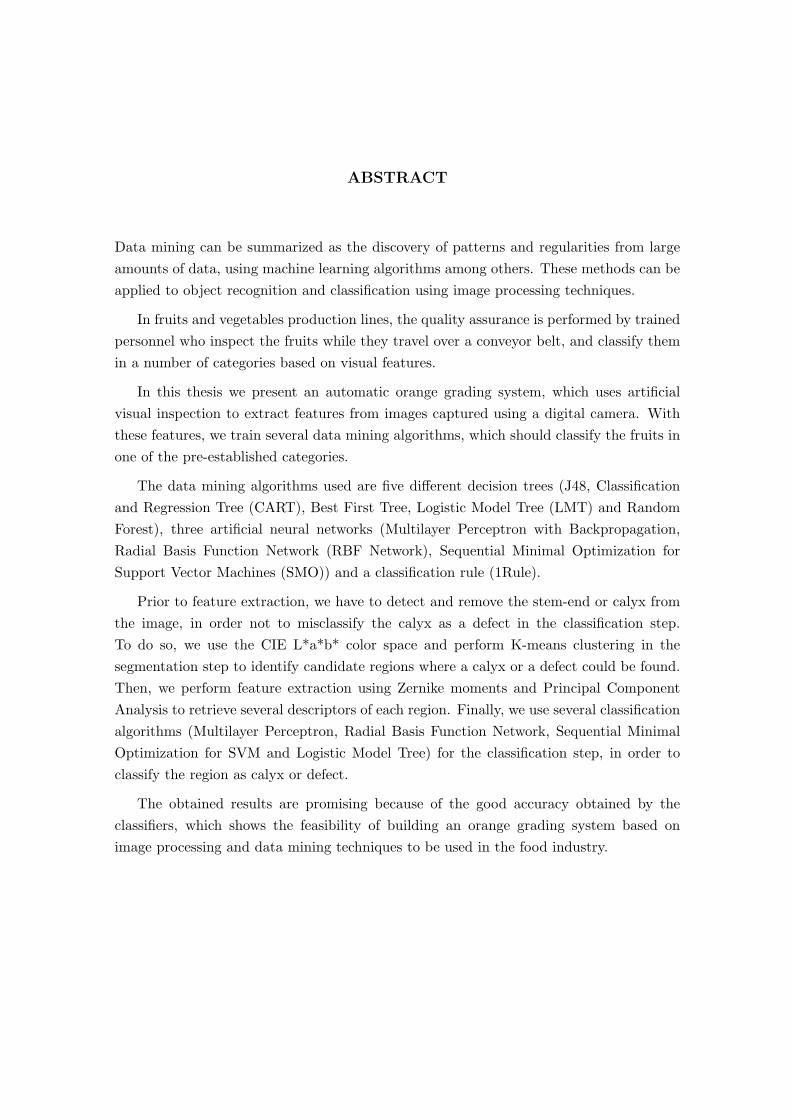
Data mining can be summarized as the discovery of patterns and regularities from large
amounts of data, using machine learning algorithms among others. These methods can be
applied to object recognition and classification using image processing techniques.
In fruits and vegetables production lines, the quality assurance is performed by trained
personnel who inspect the fruits while they travel over a conveyor belt, and classify them
in a number of categories based on visual features.
In this thesis we present an automatic orange grading system, which uses artificial
visual inspection to extract features from images captured using a digital camera. With
these features, we train several data mining algorithms, which should classify the fruits in
one of the pre-established categories.
The data mining algorithms used are five different decision trees (J48, Classification
and Regression Tree (CART), Best First Tree, Logistic Model Tree (LMT) and Random
Forest), three artificial neural networks (Multilayer Perceptron with Backpropagation,
Radial Basis Function Network (RBF Network), Sequential Minimal Optimization for
Support Vector Machines (SMO)) and a classification rule (1Rule).
Prior to feature extraction, we have to detect and remove the stem-end or calyx from
the image, in order not to misclassify the calyx as a defect in the classification step.
To do so, we use the CIE L*a*b* color space and perform K-means clustering in the
segmentation step to identify candidate regions where a calyx or a defect could be found.
Then, we perform feature extraction using Zernike moments and Principal Component
Analysis to retrieve several descriptors of each region. Finally, we use several classification
algorithms (Multilayer Perceptron, Radial Basis Function Network, Sequential Minimal
Optimization for SVM and Logistic Model Tree) for the classification step, in order to
classify the region as calyx or defect.
The obtained results are promising because of the good accuracy obtained by the
classifiers, which shows the feasibility of building an orange grading system based on
image processing and data mining techniques to be used in the food industry.

1. INTRODUCTION
1.1 Motivation
During the last years, there has been an increase in the need to measure the quality of
several products, in order to satisfy customers needs in the industry and services. In
fruit and vegetable production lines, the quality assurance is the only step which is not
done automatically. For oranges, quality assurance is performed by trained personnel who
inspect the fruits while they travel over a conveyor belt, and classify them in a number of
categories based on visual features.
Performing an accurate classification is crucial in order to fulfill the quality require-
ments established by several organizations to allow the commercialization of the fruits for
specific markets. If a good quality orange is misclassified as defective or intermediate, it
will be sold at a lower price, but if a defective orange is misclassified as good, it might
lead to the application of fines for selling defective oranges as good; or if the defect is an
illness, it can lead to discard the whole lot of fruits, causing considerable loss.
In the industry, there are very few automatic classification machines, mainly because
of the need of advanced image processing. This is required to perform fast and complex
analysis given the wide range of variations found on natural products [37].
Visual aspect is very important for fruits. An orange with an excellent peel is sold at
a higher price than another orange with the same internal features but with superficial
defects. This promoted the establishment of quality standards at many organizations For
instance, Zubrzycki & Molina [17] present a table with five categories for oranges, lemons
and tangerines. This can be seen in Table 1.1.
However, the differences in quality categories are diffuse and subjective, therefore two
orange grading experts can classify the same specimen into different categories. It is
possible to reduce this subjectivity by using an automatic classifier.

XX
XX
XX
XX
XX
XX
XX
Defect type
CategoriesExtra Cat. I Cat. II Cat. III Cat. IV
Serious defects 0% 2% 3% 4% 4%
Deep damage 0% 3% 5% 5% 5%
Overripe 0% 1% 3% 9% 9%
Total serious 0% 3% 5% 9% 9%
Deform 0% 1% 10% 20% 100%
Kind of mark
Diffuse Level 1 5% 20% 40% 100% 100%
Diffuse Level 2 0% 5% 20% 50% 100%
Deep Level 1 0% 15% 20% 3% 100%
Deep Level 2 0% 3% 10% 20% 10%
Total marks 5% 25% 40% 100% 100%
TOTAL 5% 25% 40% 100% 100%
Tab. 1.1: Citrus classification categories. Adapted from [17]
1.2 State of the Art
In the scientific community, there is significant interest in the development of artificial
vision based fruit classification systems. Recce et. al [37] introduce an orange classifier
which uses artificial neural networks and Zernike polynomials. Unay and Gosselin [10] show
an apple classifier based on color and texture features, using principal components analysis
and neural networks. Fobes [28] proposes a system to estimate the volume of a fruit from
digital images. Morimoto et al. [56] introduce a system for fruit shape recognition using
the fractal dimension and neural networks.
One of the main complications faced by the authors is the detection of the calyx,
because it can be wrongly classified as a defect [37]. Another difficulty is the speed needed
to perform the classification, because it has to be done in the time imposed by the speed
of the conveyor belt.
Several authors have studied stem-end/calyx detection with success. Unay and Gos-
selin extract several features (invariant moments of Hu, textural features of Haralick, Gray-
Level Co-occurrence Matrices, averages and ranges of coefficients of Daubichies wavelet
decomposition, averages and ranges of intensities of objects) and then compare two clas-
sifiers (K-Nearest Neighbor and Support Vector Machines) [11]. Recce et. al introduce a
stem detection system based on Zernike moments and Neural Networks [37]. Ruiz et. al
present a system which uses color segmentation and Bayesian decision rules to discriminate
the calyx and cut stem [34]. Leeman and Destain propose a pattern matching by corre-
lation approach to detect the calyxes and stem-ends. Xing, Jancsok and Baerdemaeker
2

perform Principal Component Analysis (PCA) for stem end/calyx detection of apples,
where they analyze the contour features of the first principal component score images [20].
In this thesis, we present a method to classify oranges using digital still images. The
process consists of the extraction of relevant features to be able to classify the orange into
three categories (good, intermediate and defective). Some of the most relevant features
used are statistical descriptors, histogram analysis, and the fractal dimension (FD), which
can be used to characterize the oranges’ peel smoothness as a quality indicator.
The method developed in this thesis is exclusively focused in the calyx detection and
classification steps, but in order to make this thesis self contained, in chapter 3 we briefly
introduce the system that should be used to capture the images.
The results of this thesis have been presented in [25], [23] and [24].
1.3 Thesis Organization
This thesis is organized in the following way: we start by presenting the fundamentals of
digital image processing and data mining in chapter 2, where we explain in detail all the
machine learning algorithms used in this thesis. In chapter 3, a general description of the
system is made, introducing the image capture step.
Next, the calyx detection subsystem is analyzed in chapter 4, where we explain the
segmentation process, the feature extraction algorithms involved, and the classification of
candidate regions as calyx or defect using data mining algorithms.
In chapter 5 we focus on the quality categories classification subsystem, explaining how
the features used by the data mining algorithms in the classification step are obtained,
and in section 5.2 we present the classification results obtained with the experiments.
Finally, in chapter 6 we present the conclusions and future works.
3
2. PRELIMINARIES
In this chapter we introduce the fundamentals of digital image processing and data mining
in order to give the reader a background on these techniques and make this thesis self
containing. If the reader has knowledge on these concepts, this chapter could be skipped.
2.1 Digital Image Processing
2.1.1 Digital Image Representation
An image can be represented as a two dimensional function f : R2 → R, f(x, y), being x
and y the spatial coordinates and the value of f at a certain point is the intensity of the
image in that point. A digital image is an image f : N × N → [0, 1, ..., L − 1] where L is
the luminance value [49]. The processing of this kind of images is named ’Digital Image
Processing’.
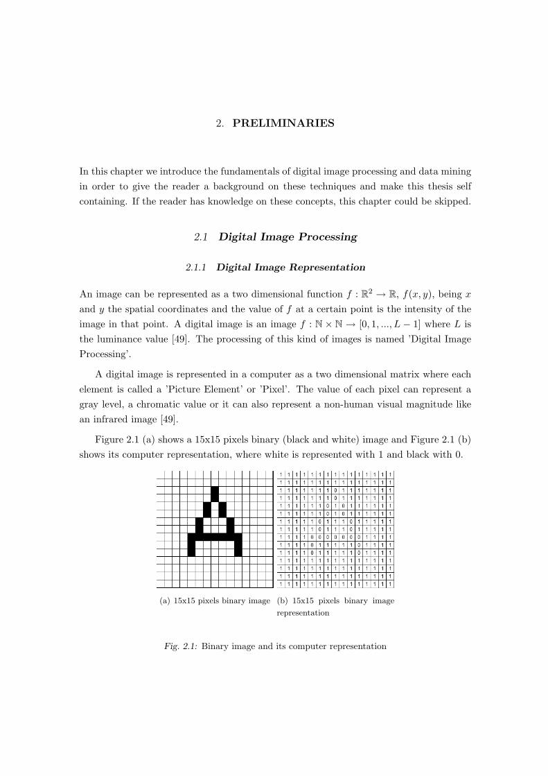
A digital image is represented in a computer as a two dimensional matrix where each
element is called a ’Picture Element’ or ’Pixel’. The value of each pixel can represent a
gray level, a chromatic value or it can also represent a non-human visual magnitude like
an infrared image [49].
Figure 2.1 (a) shows a 15x15 pixels binary (black and white) image and Figure 2.1 (b)
shows its computer representation, where white is represented with 1 and black with 0.
(a) 15x15 pixels binary image (b) 15x15 pixels binary image
representation
Fig. 2.1: Binary image and its computer representation

Fig. 2.2: Additive model of light: Adding Red and Green forms Yellow, Red and Blue form Ma-
genta, Blue and Green form Cyan and adding Red, Green and Blue form white
Color images can be represented in different ways, according to the color space being
used. This will be explained in the following section.
2.1.2 Color Spaces
Color images are represented as a combination of matrices where each matrix represent a
single color component image.
• Red, Green and Blue (RGB) Color Space: Red, Green and Blue are the colors
basis of light, so it is widely used in image acquisition using photo and video cameras,
and also for displaying images in computer monitors and projectors. An example of
additive colors is shown in Figure 2.2. A RGB image consists of three components:
Red, Green and Blue, so each pixel has three values. This can be seen in Figure 2.3.
Figure 2.4 shows the Red, Green and Blue components of an image of size 144x192
with 8 bits per channel (or component), so each pixel can contain 256 (28) levels for
each component.
• Cyan, Magenta, Yellow, Black (CMY K) Color Space: Cyan, Magenta and
Yellow are the colors basis for pigments, and the secondary colors of light, because
they subtract the color from the reflected light. For example, Cyan is the absence of
Red, Magenta the absence of Green and Yellow the absence of Blue [49]. An example
of subtractive colors is shown in Figure 2.5.
The formula to convert from RGB to CMY is shown in Equation (2.1).
Theoretically, equal amounts of pigments of cyan, magenta and yellow should pro-
duce black, but in practice it produces a kind of gray, so black (K) is also added [49].
5
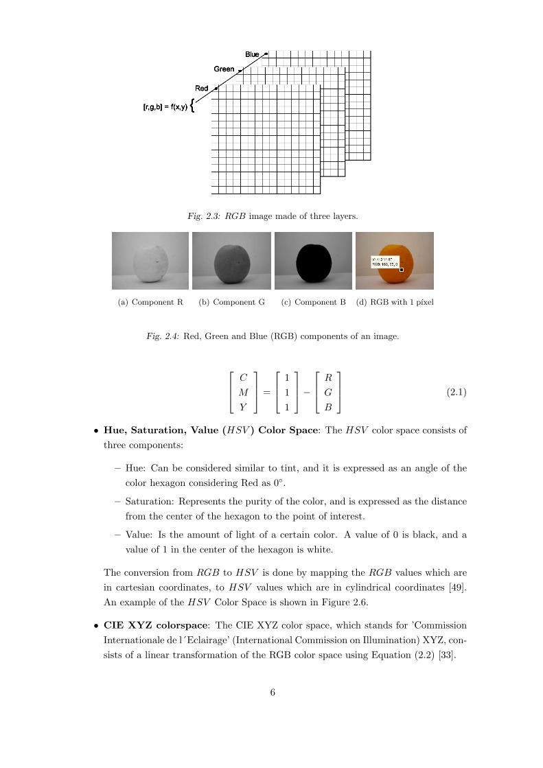
Fig. 2.3: RGB image made of three layers.
(a) Component R (b) Component G (c) Component B (d) RGB with 1 pıxel
Fig. 2.4: Red, Green and Blue (RGB) components of an image.
C
M
Y
=
1
1
1
−
R
G
B
(2.1)
• Hue, Saturation, Value (HSV ) Color Space: The HSV color space consists of
three components:
– Hue: Can be considered similar to tint, and it is expressed as an angle of the
color hexagon considering Red as 0◦.
– Saturation: Represents the purity of the color, and is expressed as the distance
from the center of the hexagon to the point of interest.
– Value: Is the amount of light of a certain color. A value of 0 is black, and a
value of 1 in the center of the hexagon is white.
The conversion from RGB to HSV is done by mapping the RGB values which are
in cartesian coordinates, to HSV values which are in cylindrical coordinates [49].
An example of the HSV Color Space is shown in Figure 2.6.
• CIE XYZ colorspace: The CIE XYZ color space, which stands for ’Commission
Internationale de l´Eclairage’ (International Commission on Illumination) XYZ, con-
sists of a linear transformation of the RGB color space using Equation (2.2) [33].
6

Fig. 2.5: Subtracting Colors of light: Subtracting magenta and cyan from white forms blue, sub-
tracting magenta and yellow from white forms red, subtracting cyan and yellow from
white forms green, and subtracting cyan, magenta and yellow forms black
X
Y
Z
=
0.6079 0.1734 0.2000
0.2990 0.5864 0.1146
0.0000 0.0661 1.1175
·
R
G
B
(2.2)
• CIE L*a*b* colorspace: The CIE L*a*b* color space was designed to be percep-
tually uniform, so it is considered as one of the best color spaces for matching the
human perception distance of colors [14].
The color space consists of three layers:
– Luminance or brightness layer L∗: Can have the range from 0 to 100, where 0
is black and 100 white. It does not contain color information.
– Red-Green chromatic layer a∗– Blue-Yellow chromatic layer b∗ [26]
An example of CIE L*a*b* components is shown in Figure 2.7, where 2.7 (a) shows
the luminance component of the image, 2.7 b) and 2.7 c) show the a and b components
and Figure 2.7 d) shows both the a and b components which include all the color
information, discarding the luminance information.
CIE L*a*b* is based on the XY Z color space, so conversion from RGB to CIE
L*a*b* is performed with the following equations: First, convert from RGB to
XY Z using Equation (2.2).
Then, convert from XY Z to L*a*b* using Equation (2.3).
7

Fig. 2.6: HSV Color Space.
a∗ = 500 ∗ [f(X/Xn) − f(Y/Yn)]
b∗ = 200 ∗ [f(Y/Yn) − f(Z/Zn)]
L∗ =
116 ∗ (Y/Yn)1/3 − 16 when (Y/Yn) > 0.008856,
903.3 ∗ (Y/Yn) otherwise.
(2.3)
where Xn, Yn and Zn are the values of reference for white (e.g.: Xn = 1, Yn = 0.9872
and Zn = 1.18225) [33].
(a) Luminance (b) Component a∗ (c) Component b∗ (d) Components a∗ & b∗
Fig. 2.7: Luminance, a∗ and b∗ (CIE L*a*b*) components of an image
8

2.1.3 Morphological operators
Morphological operators are primarily used with binary images to recover shapes of the
image, which may be needed to describe the shape of the objects of interest [49].
In this section we explain the basic morphological operators used in this thesis.
• Dilation: Dilation consists in growing the objects by expanding their boundaries
in a controlled way using a structuring element, which is the shape used to perform
the operation [49]. The mathematical equation is the following:
G ⊕ M = {p : Mp ∩ G 6= ⊘}. (2.4)
where M is the set of non-zero mask pixels known as the structuring element, G
is the original image consisting of the set of all non zero pixels of the matrix, p is
the reference pixel (generally the center of the structuring element) and Mp is the
structuring element shifted to the reference point p [21].
The equation means that dilation of G using M results in all structuring elements
which overlap with G at least in one point [49].
An example of dilation operation can be seen in Figure 2.8 (c).
• Erosion: Erosion is the opposite to dilation, as the object is ’shrunk’ or ’thinned’
instead of grown. It also uses a structuring element, and the equation is denoted by:
G ⊖ M = {p : Mp ∩ Gc 6= ⊘ }. (2.5)
which means that the resulting object will have a foreground value (e.g.: 1) in
the center of the structuring element (p) only when it does not overlap with the
background [49].
An example of erosion is shown in Figure 2.8 (d).
• Opening: Morphological opening of G by M consists of performing erosion of G by
M and that result dilated by M . In mathematical notation, opening is denoted by:
G ◦ M = (G ⊖ M) ⊕ M (2.6)
and the result of morphological opening is an object which has been removed all the
regions that cannot contain the structuring element M . Opening is commonly used
to remove background noise, smooth object contours, break thin connections and
remove thin protrusions [49].
An example of the application of morphological opening operation is shown in Fig-
ure 2.8 (e), where it can be seen that the three regions in white are kept.
• Closing: Closing consists of dilation followed by erosion and the mathematical
equation is the following:
G • M = (G ⊕ M) ⊖ M (2.7)
9

(a) Original image with background
removed
(b) Binary representation of the im-
age
(c) Morphological dilation (d) Morphological erosion
(e) Morphological closing (f) Morphological opening
Fig. 2.8: Morphological operators
10

and similar to opening, closing smooths contours. However, it joins narrow breaks,
fills long thin gulfs and fills holes smaller than the structuring element M [49].
An example of applying the closing operation is shown in Figure 2.8 (f), where it
can be seen that only the biggest of the three regions is kept, as closing fills holes
smaller than the structuring element, in which in this case has a size of 8 pixels and
a circular shape.
Closing and opening can also be combined and are commonly used to remove noise.
11

2.2 Data Mining and Knowledge Discovery in Databases
Data mining can be defined as the discovery of patterns and regularities from large amounts
of data, using machine learning algorithms among others. Another definition of Data
mining given by [18] is:
’Data mining is the extraction of implicit, previously unknown, and potentially
useful information from data.’
Data mining involves learning in a practical, not theoretical, way, where existing data takes
the form of examples, and the output of the process is the prediction of new examples [18].
Data mining is also one step in the Knowledge Discovery in Databases (KDD) process.
The steps involved in the KDD process are the following [16]:
1. Data Cleaning: Remove inconsistencies and noise.
2. Data Integration: Consolidate in a single data source data spread over different
databases.
3. Data Selection: Irrelevant data for the task is discarded.
4. Data Transformation: Data are transformed for mining like performing aggrega-
tions or summarizations.
5. Data Mining: the process of discovering patterns and regularities from data, using
machine learning algorithms among others.
6. Pattern Evaluation: the data mining step may generate several patterns or mod-
els, which should be evaluated in order to keep the most interesting ones. A pattern is
considered interesting if it is valid on new data, it is potentially useful and novel [16].
Jan & Kamber [16] also mention that a pattern is interesting if it is easily under-
stood by humans, something that for us is desirable, but depending on the task
involved, it may not be so necessary and several machine learning algorithms like
neural networks, which are very difficult to interpret by humans, are widely used.
7. Knowledge Representation: The representation of the discovered knowledge to
the user, where information visualization techniques are applied.
Data mining is commonly used as a predictive tool, or as a descriptive tool used to
describe the properties of the data [16]. The main functionalities of data mining are the
following [16]:
• Characterization and description: Data characterization consists in describ-
ing the general features of the elements of a class, like for example describing the
12

characteristics of oranges that belong to CAT I. Data discrimination resides in de-
scribing classes by comparing a class against other different classes and computing
the differences.
• Association analysis: Resides in finding attribute-value relations that occur to-
gether. It is mainly used in market basket analysis and transaction data analysis.
Association rules are used for this purpose. For example, an association rules analy-
sis in a supermarket may find that sausages and hot dog bread are bought together
with a confidence of 90% (the probability of buying both items together) and a
support of 30% (30% of all the transactions contains both).
• Classification and prediction: Classification consists in finding a model (using
training data) that describes the data and when a new example with an unknown
class is input, its class is predicted. Classification is explained in section 2.2.1.
• Cluster analysis: Cluster analysis consists in grouping similar elements in a cluster.
It uses unsupervised learning because the nature of the class of the elements is not
known in advance.
• Outlier analysis: Outliers are data elements that differ considerably from the
rest of the elements in the dataset. In most cases outliers are a result of noisy or
incorrect data, or it might be a valid value which, depending on the task, it might
be worthwhile to analyze. For example, outliers are commonly used when detecting
frauds.
• Evolution analysis: can be applied to all the previous items when dealing with
objects with time variant behavior, such as stock market trends, where time-series
analysis is commonly used.
2.2.1 Classification using machine learning algorithms
In order to associate the features of the image with the corresponding class (good, in-
termediate or defective), we use several data mining Algorithms. For this purpose, we
experiment with most of the algorithms available in the Waikato Environment for Knowl-
edge Analysis (WEKA) software which are suitable for the kind of problem presented in
this thesis, and choose the ones with the highest accuracy.
The chosen algorithms are: five different decision trees (J48, Classification and Re-
gression Tree (CART), Best First Tree, Logistic Model Tree (LMT) and Random Forest),
three artificial neural networks (Multilayer Perceptron with Backpropagation, Radial Basis
Function Network (RBF Network), Sequential Minimal Optimization for Support Vector
Machines (SMO)) and a decision rule (1Rule).
Before giving the definition of classification, we have to define some concepts like ’class’
and ’hypothesis’ in order to fully understand the following paragraphs.
13

There exist three definitions for class:
1. Classes as labels for different populations: in this case, members of each population
are assigned to different classes, and membership to that group is not in question (e.g.
dogs and cats). The allocation to a certain class, which is done by the supervisor, is
independent of the attributes [41].
2. Classes are the result of a prediction problem: For example, to determine if tomorrow
will rain (class = 1) or not (class = 0). This class is predicted based on knowledge
of the attributes [41].
3. The class is a function of the attributes: For example, to determine if an item is
faulty, there exists a rule which already classified items as faulty if certain attributes
are out of a certain limit [41]. The goal is to create a rule which resembles the
original one.
In our problem, we consider the class as a function of the attributes (definition N◦ 3)
because there exists a rule used by the people who manually classify the fruit, and this
rule is the one that has to be mimicked.
According to [41], classification can be related to supervised and unsupervised learning.
In unsupervised learning, given a set of observations, the algorithm has to group the
instances into classes or clusters based on similarity criteria [16]. On the other hand, in
supervised learning we already know the class c of each observation in the dataset D of
size m. The aim is to find a hypothesis or rule, h, that satisfies c for the members of D
and will be a good guess for c when we have to classify a new observation [44], [41].
Another important aspect in machine learning is concept learning. In machine learning,
the concept is ’the thing to be learned ’ [18]. According to [36], Concept Learning means
to infer a boolean-valued function from training examples of its input and output, so it
can be seen as a searching problem through a predefined space of potential hypothesis to
determine the hypothesis which best fit the training examples.
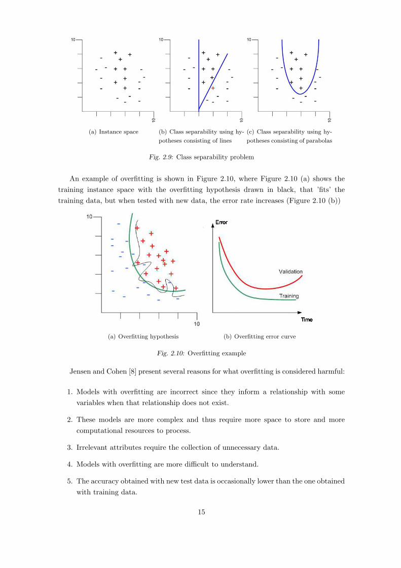
Figure 2.9 (a) shows an instance space example which consists of points in the x,y
plane. In Figure 2.9 (b), a hypotheses consisting of lines is able to separate the classes but
one instance is misclassified. Figure 2.9 (c) shows an hypothesis consisting of a parabola,
which can perfectly classify the instances without error.
Overfitting: One important aspect that has to be considered when building ma-
chine learning algorithm is overfitting, which is a very common pathology of induction
algorithms [8, 41].
Overfitting occurs when inferring more structure from the training set than is justified
by the population from which it is drawn [41]. These added components do not improve
accuracy when tested with new data samples [8].
14
(a) Instance space (b) Class separability using hy-
potheses consisting of lines
(c) Class separability using hy-
potheses consisting of parabolas
Fig. 2.9: Class separability problem
An example of overfitting is shown in Figure 2.10, where Figure 2.10 (a) shows the
training instance space with the overfitting hypothesis drawn in black, that ’fits’ the
training data, but when tested with new data, the error rate increases (Figure 2.10 (b))
(a) Overfitting hypothesis (b) Overfitting error curve
Fig. 2.10: Overfitting example
Jensen and Cohen [8] present several reasons for what overfitting is considered harmful:
1. Models with overfitting are incorrect since they inform a relationship with some
variables when that relationship does not exist.
2. These models are more complex and thus require more space to store and more
computational resources to process.
3. Irrelevant attributes require the collection of unnecessary data.
4. Models with overfitting are more difficult to understand.
5. The accuracy obtained with new test data is occasionally lower than the one obtained
with training data.
15

2.2.2 K-Means cluster analysis
Cluster analysis is the process of grouping similar objects in the same class [16]. The
similarity of two objects is determined by measuring the distance between them, which
can be calculated in different ways, like Euclidean distance, normalized Euclidean distance,
Mahalanobis distance, etc. [12].
The Euclidean distance ers between two points xr and xs is denoted by:
ers =√
(xr − xs)′(xr − xs) (2.8)
And the Mahalanobis distance mrs between xr and xs is computed with the following
equation:
mrs =√
(xr − xs)′Σ−1(xr − xs) (2.9)
being Σ an estimated variance-covariance matrix [12].
This thesis uses Euclidean distance. Cluster analysis belongs to the unsupervised
learning group of algorithms, because the class of each individual is not known.
The clustering method used in this thesis is k-means. This algorithm requires to be
indicated the number of clusters (k) to build, and performs an iterative process producing
k groups of elements whose inter-cluster distance is minimum. The center of each cluster
is called the ’center of mass’ and is the mean value of the elements of the cluster it belongs
to [16].
The k-means algorithm can be described in these steps:
1. Randomly select k elements which will be used as the initial centers.
2. Assign each of the remaining elements to the cluster which similarity (distance) to
the center is minimum.
3. Compute the new mean (center) of each cluster.
4. Repeat steps b) and c) until a stop criteria is met (i.e.: mean square error).
An example of k-Means clustering can be seen in Figure 2.11.
2.2.3 Decision Trees
Jan & Kamber [16] define a decision tree as a tree structure like a flow diagram, in which
each node indicates a test on an attribute, each branch represents the result of that test
and the leaf nodes represent classes.
Mitchell [36] argues that a decision tree is a method that is used to perform approxi-
mations when the objective functions are discrete. An advantage of the decision trees is
16
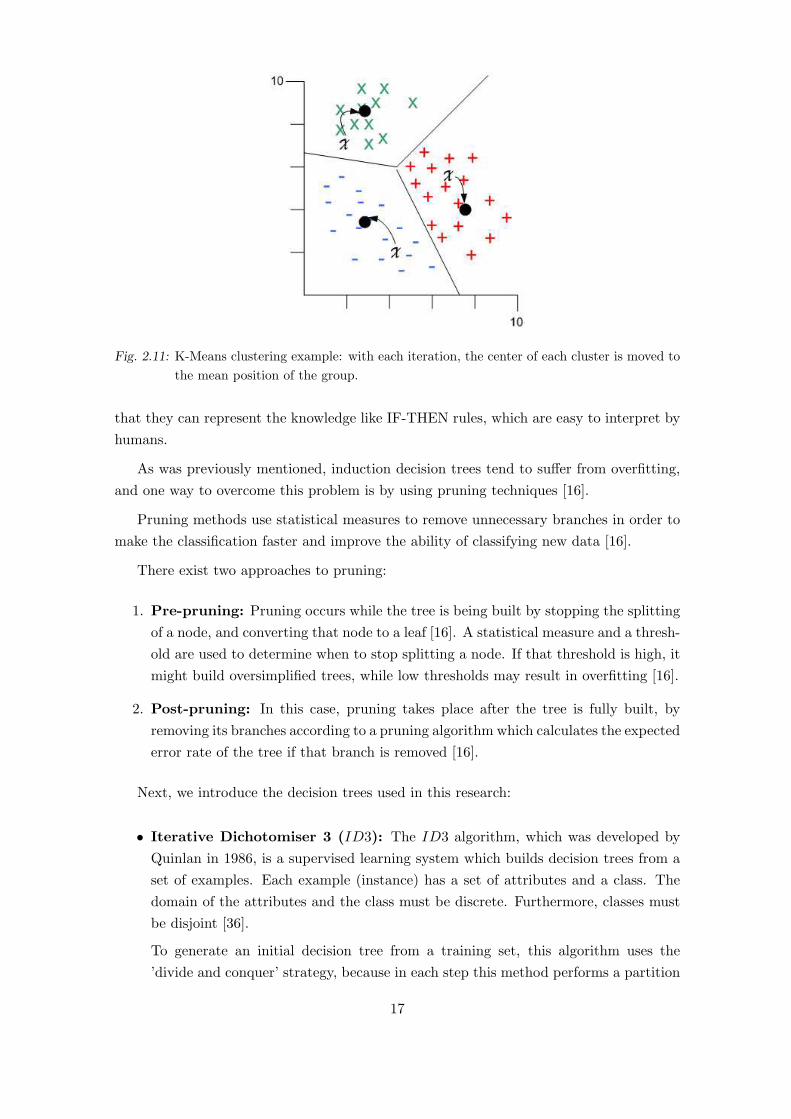
Fig. 2.11: K-Means clustering example: with each iteration, the center of each cluster is moved to
the mean position of the group.
that they can represent the knowledge like IF-THEN rules, which are easy to interpret by
humans.
As was previously mentioned, induction decision trees tend to suffer from overfitting,
and one way to overcome this problem is by using pruning techniques [16].
Pruning methods use statistical measures to remove unnecessary branches in order to
make the classification faster and improve the ability of classifying new data [16].
There exist two approaches to pruning:
1. Pre-pruning: Pruning occurs while the tree is being built by stopping the splitting
of a node, and converting that node to a leaf [16]. A statistical measure and a thresh-
old are used to determine when to stop splitting a node. If that threshold is high, it
might build oversimplified trees, while low thresholds may result in overfitting [16].
2. Post-pruning: In this case, pruning takes place after the tree is fully built, by
removing its branches according to a pruning algorithm which calculates the expected
error rate of the tree if that branch is removed [16].
Next, we introduce the decision trees used in this research:
• Iterative Dichotomiser 3 (ID3): The ID3 algorithm, which was developed by
Quinlan in 1986, is a supervised learning system which builds decision trees from a
set of examples. Each example (instance) has a set of attributes and a class. The
domain of the attributes and the class must be discrete. Furthermore, classes must
be disjoint [36].
To generate an initial decision tree from a training set, this algorithm uses the
’divide and conquer’ strategy, because in each step this method performs a partition
17

of the data of the node according to a test performed over the most discriminative
attribute [38].
The criteria used by ID3 to split the nodes is the Entropy. Entropy can be seen
as the amount of information existing in the result of an experiment [44]. Thus,
the ID3 algorithm chooses, for each decision node, the attribute with the high-
est discriminating capacity over the examples analyzed, which is the attribute that
generates disjoint sets where the internal homogeneity is maximized (the variability
minimized) with respect to the values of the class [44].
• C4.5 and J48 decision Trees: C4.5 was presented by Quinlan in 1993 as an
extension of ID3 [38]. The splitting criteria used by this algorithm is the gain
ratio. It also allows the possibility of performing a pessimistic post pruning of the
resulting tree (substituting a subtree by a leave, or by one of its branches) [6]. The
construction strategy is similar to ID3.
The gain ratio criterion consists in building decision trees that use keys to make
branches. It has been observed that this criterion tends to build unbalanced trees,
a characteristic which inherits from the splitting rule that it derives (information
gain). Both heuristics are based on an entropy measure which favors partitions of
the training set unequal in size when one of them has all the instances belonging
to the same class, despite only few instances of the training set belong to that
partition [6].
The J48 algorithm is a new version of Quinlan’s C4.5 algorithm which is used in the
data mining software WEKA. An example of a J48 tree is shown in Figure 2.12.
Fig. 2.12: J48 Decision tree for the Iris dataset
• Classification And Regression Trees (CART): Classification And Regression
Trees is a method created by Breiman [31] that produces decision trees from cate-
gorical or continuous variables. If the variables are continuous, it makes a regression
tree, and if they are categorical, it makes a classification tree. The splitting crite-
ria used for classification are the Gini index, Chi-squared and G-squared; while the
18

splitting criteria used for regression is a least squared deviation criterion [31]. The
trees obtained using this method are binary [6].
This algorithm also allows to perform a cost-complexity pruning with cross-
validation [6].
• Best First Tree: Unlike traditional decision trees (i.e., C4.5, CART) which expand
in depth, Best First trees expand selecting the node which maximizes the impurity
reduction among all the available nodes to split. The impurity measure used by this
algorithm is the Gini index and information gain [51].
• Logistic Model Tree (LMT): is a decision tree with the peculiarity that each
leave is a logistic regression model [42]. While logistic regression only captures
lineal patterns, decision trees generate non linear models. One of the disadvantages
of this method is the increased computational complexity [42]. An example of a
Logistic Model Tree which was generated in the calyx detection process is shown in
Figure 2.13, where it can be seen that the leaves of the tree are logistic regressions.
Fig. 2.13: Logistic Model Tree example for calyx detection
• Random Forest: generates a series of decision trees, where each tree is built using a
vector generated randomly for each tree, but using the same distribution for all trees.
After building a considerable amount of trees, each one votes for the most popular
class, and the final model classifies with the class voted by the majority [30]. One
interesting aspect of this classifier is that, given the law of large numbers, overfitting
is not produced [30].
19
2.2.4 Classification Rules
• One Rule (1R): The One Rule (1R) algorithm makes a classification rule applying
only a single attribute, producing a result similar to a single level decision tree [50].
This method makes very simple models and has been proved that with several data
sets, it shows results as good as the ones achieved with more complex methods like
C4.5 decision trees [50].
2.2.5 Artificial Neural Networks (ANN)
A neural network can be seen as a massively parallel distributed processor, made of
simple processing units, which are capable of storing experimental knowledge and
have it ready to be used later [52].
It resembles the human brain in which the knowledge is obtained from the environ-
ment through a learning process, and the neural interconnection strengths, known
as synaptic weights, are used to store the acquired knowledge [52].
Biological brains are composed by neurons, which are cells that can process informa-
tion. An example of a biological neuron is shown in figure 2.14 (a), where it can be
seen that the structure of the cell consists of the cell body, the nucleus and a series
of connectors named dendrites which are responsible for receiving the impulse from
predecessor neurons. The axon transmits the impulse to the axon terminal branches
where the synapses takes place transmitting the neuron’s output to other neuron’s
dendrites through a chemical process [52].
The artificial counterpart, which diagram is shown in Figure 2.14 (b), has a series of
input signals (equivalent to dendrites), synaptic weights (equivalent to the synapses),
an activation function (equivalent to the cell body) and the output of the neuron [19].
The mathematical formula of an artificial neuron is denoted by:
yk = ϕ(
n∑
j=1
wkjxj + bk) (2.10)
where wk1..wk1n are the synaptic weights, x1..xn are the input signals, bk is the bias,
ϕ(.) is the activation function and yk is the output signal. The bias bk is used to
move the threshold of the activation function [52].
The activation function ϕ(.) : R → R has the effect of limiting the amplitude of the
output of the neuron. Examples of activation functions are shown in Figure 2.15.
Artificial Neural Networks are useful in pattern recognition applications, such as
visual inspection systems, where the human brain outperforms computer systems.
For example, [36] mentions that although human brains switching speed is about
10−3 seconds while computer’s switching speed is in the order of 10−10 seconds,
it takes only 10−1 seconds for a human to visually recognize his mother. This
20

(a) Biological neuron structure
(b) Artificial neuron diagram
Fig. 2.14: Biological and Artificial neurons
behaviour is thought to be achieved by the distributed representation and highly
parallel processing of the human brain, and this is the motivation of artificial neural
networks architecture [36].
However, there exist several differences between Artificial Neural Networks and bi-
ological brains, like the hormones flow that is not modeled in ANNs, or the fact
that ANN output a single constant value while biological neurons output a series of
complex time series of spikes [36].
• Multilayer Perceptron Neural Network with Backpropagation (MLP):
The ’Multilayer Perceptron’ neural network has an input layer made of input nodes
or ’sensory units’, one or many hidden layers and an output layer. During the train-
ing step, the input signal spreads forward from the input layer to the output layer,
producing a result. This result is compared to the desired value and errors are calcu-
lated in the opposite direction while the synaptic weights are adjusted. Due to this
error propagation process from the output layer to the input layer, this algorithm is
known as ’Backpropagation’
21

(a) Threshold activation function (b) Piecewise linear activation function
(c) Sigmoid activation function
Fig. 2.15: Activation functions
• Radial Basis Function Network (RBF Network): Unlike the multilayer per-
ceptron with backpropagation algorithm which uses a recursive approximation tech-
nique known as stochastic approximation, the RBF network can be seen as a curve
fitting problem in a high dimension space, where it has to find the best surface to
fit the training data [52]. The network has three layers. The first layer is the input
from the outside, the second is a hidden layer that makes a non linear transforma-
tion from the input space to the high dimension hidden space. The third layer is the
output layer and shows the response of the neural network to the input data [52].
• Sequential Minimal Optimization for Support Vector Machines (SMO):
Support Vector Machines are linear classifiers that learn in a batch mode basis. The
learned classifier consists of an hyperplane, and the classification is performed by
computing the sign of the dot product of the data point with the classifier [53].
During the training of a support vector machine, it is required to find the solution
to a large quadratic programming (QP ) problem. The SMO algorithm divides this
problem into many smaller QP problems, and they are solved analytically requiring
fewer computational cost [47].
2.2.6 Attribute selection methods
Despite most data mining algorithms are capable of getting rid of non discriminant
attributes, in many cases better results are obtained if the dataset is previously
processed with attribute subset selection algorithms. Furthermore, algorithms often
get their speed reduced by irrelevant or redundant data, which can be discarded
in an early stage by applying attribute selection methods before training the main
machine learning algorithm [40].
22

In the following paragraphs, we briefly explain each of the attribute selection methods
used in this thesis.
– Correlation based feature subset selection (CFSSubset): This method
consists in the evaluation of the worth of a subset of attributes taking into con-
sideration the individual predictive power of each attribute and the degree of
redundancy between them [40]. By removing irrelevant attributes, the hypoth-
esis search space is reduced, and in some algorithms, the required storage gets
also reduced. Hall and Smith describe the hypothesis in which the heuristic
is based as: ’Good feature subsets contains features highly correlated with the
class, yet uncorrelated with each other’ [40].
– Information Gain attribute evaluation: This method uses information
theory to measure the information gain of each attribute in order to determine
the discriminant level of each attribute with respect to the class. [18].
– Chi Squared Attribute Evaluator for features subset selection: This
method uses the Chi Squared statistic to evaluate the importance of each at-
tribute with respect to the class [18].
2.2.7 Classifier performance evaluation
In classification problems with only two classes, each instance I of the data set is evaluated
an mapped to one of the classes: p (positive) or n (negative) [55]. The result of the
classification can be either correct or wrong, so there are four possibilities:
1. TP : A true positive is when a positive instance is correctly classified as positive
2. TN : A true negative is when a negative instance is correctly classified as negative
3. FP : A false positive is when a negative instance is wrongly classified as positive
4. FN : A false negative is when a positive instance is wrongly classified as negative
The combination of these values are presented in a matrix form, known as the Con-
fusion Matrix, like the one shown in Table 2.1
``
``
``
``
``
``
``
``
True class
Predicted classPositive Negative
Positive TP FN
Negative FP TN
Tab. 2.1: Confusion matrix example
Classifier performance can be evaluated by different metrics:
23

• Accuracy: TP+TNTP+TN+FP+FN
• Precision: TPTP+FP
• False positive rate (hit rate): FPFP+TN
• True positive rate=Recall: TPFN+TP
• F-measure: 21/precision+1/recall
• Error rate 1 − accuracy
As predictive accuracy has been widely used as the main evaluation criterion [32], we
use this metric to compare classifier performance.
However, there exist better ways to measure the performance of a classifier. The area
under the ROC (receiver operating characteristics) curve (AUC) is considered by many
authors a much better metric than accuracy for evaluating learning algorithms [32].
One of the reasons why classification accuracy is not always suitable resides in the fact
that accuracy assumes equal misclassification costs, and most of the real time problems
fail in this assumption [15]. Furthermore, accuracy maximization assumes that class priors
are known for the target environment [15].
The AUC metric not only overcomes these drawbacks, it also has increased sensitivity
in ANOVA tests and is independent to the decision threshold [32]. ROC curves have also
the advantage that describe the predictive behavior of the classifier independent of class
distribution or error costs [15].
We use the AUC metric to compare classifiers performance when predicting two class
problems (calyx detection and orange quality classification in two classes).
An example of a ROC curve is shown in Figure 2.16, where it can be seen that a ROC
plot has two axis: The true positive rate TP is drawn in the Y axis, and the false positive
rate FP is drawn in the X axis. Note that a confusion matrix corresponds to one point
in the ROC curve [55].
24
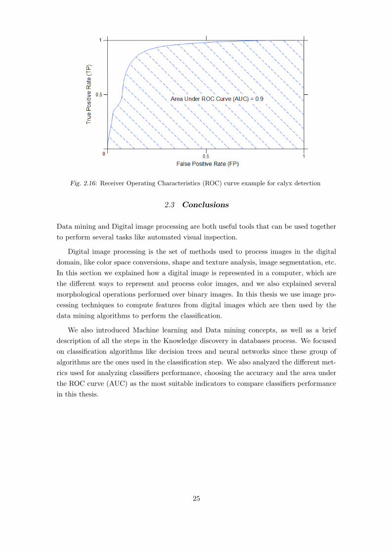
Fig. 2.16: Receiver Operating Characteristics (ROC) curve example for calyx detection
2.3 Conclusions
Data mining and Digital image processing are both useful tools that can be used together
to perform several tasks like automated visual inspection.
Digital image processing is the set of methods used to process images in the digital
domain, like color space conversions, shape and texture analysis, image segmentation, etc.
In this section we explained how a digital image is represented in a computer, which are
the different ways to represent and process color images, and we also explained several
morphological operations performed over binary images. In this thesis we use image pro-
cessing techniques to compute features from digital images which are then used by the
data mining algorithms to perform the classification.
We also introduced Machine learning and Data mining concepts, as well as a brief
description of all the steps in the Knowledge discovery in databases process. We focused
on classification algorithms like decision trees and neural networks since these group of
algorithms are the ones used in the classification step. We also analyzed the different met-
rics used for analyzing classifiers performance, choosing the accuracy and the area under
the ROC curve (AUC) as the most suitable indicators to compare classifiers performance
in this thesis.
25
3. SYSTEM OVERVIEW
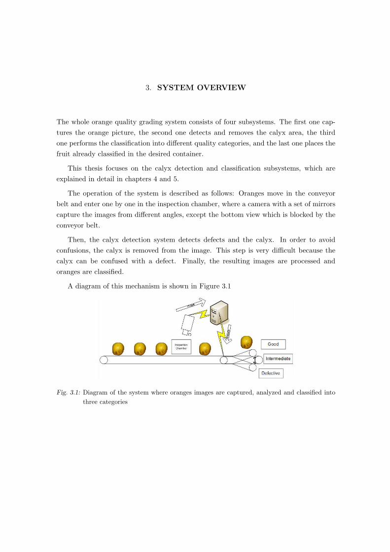
The whole orange quality grading system consists of four subsystems. The first one cap-
tures the orange picture, the second one detects and removes the calyx area, the third
one performs the classification into different quality categories, and the last one places the
fruit already classified in the desired container.
This thesis focuses on the calyx detection and classification subsystems, which are
explained in detail in chapters 4 and 5.
The operation of the system is described as follows: Oranges move in the conveyor
belt and enter one by one in the inspection chamber, where a camera with a set of mirrors
capture the images from different angles, except the bottom view which is blocked by the
conveyor belt.
Then, the calyx detection system detects defects and the calyx. In order to avoid
confusions, the calyx is removed from the image. This step is very difficult because the
calyx can be confused with a defect. Finally, the resulting images are processed and
oranges are classified.
A diagram of this mechanism is shown in Figure 3.1
Fig. 3.1: Diagram of the system where oranges images are captured, analyzed and classified into
three categories

3.1 Image capture
The image capture system consists of a conveyor belt and an inspection chamber where
images are captured by a digital camera. The main difficulty of capturing the image is to
be able to capture the picture from all angles, without loosing any section of the orange’s
skin.
There exist many alternatives for solving the problem of not being able to capture the
bottom view.
One solution to solve this inconvenient is the one proposed by Recce et al. [37]. They
suggest that the fruit travel over a conveyor belt at a known constant speed, which throws
the fruit in the air to perform the capture from all possible angles. This method is
illustrated in Figure 3.2 (a).
(a) The fruit is thrown in the air while a camera captures
the images from all possible angles
(b)
Peel-
ing
(c) Mirrors
Fig. 3.2: Different approaches of capturing images from different angles.
The disadvantage of this solution is the increased complexity to synchronize the shoot-
ing time to capture the image, with the position of the orange in the air.
Another solution is the one proposed by D’Amato et. al where they ’virtually peel’
an apple by using a video camera which captures between 3 and 5 images of the same
fruit while it is being rotated by the cilindres of the conveyor belt [45]. By doing this,
each image contains a picture of the fruit from different angles. Finally, all images are
put together (removing redundant data) and that image is the one used for processing.
27

A sample image is shown in Figure 3.2 (b). A similar approach is employed by [46] but
using more images of the same fruit to perform a cylindrical projection approximation.
A third approach employed in [28] consists in using several mirrors to capture images
from different angles, as if multiple cameras were used. One of the disadvantages we find
in this approach is that, depending on where the defect is located, it may appear reflected
in more than one mirror, increasing the chances of downgrading that specimen.
In our experiment, we capture the images manually using a digital camera and using
three mirrors to obtain images from different angles.
3.2 Classified oranges placement
Once a fruit is classified, the system has to take an action according to the obtained results.
The machine consists of a series of gates placed at the end of the conveyor belt to divert
the fruit according to the classified quality level, and deposit it in the desired container.
3.3 Conclusions
Along this chapter we showed an overview of the orange grading system, and we explained
the image capture and classified oranges placement subsystems, which are the subsystems
that are not part of the main topic of this thesis. We have discussed the inconvenients faced
when acquiring the image and the advantages and disadvantages of the solutions proposed
by different authors found in the literature. After analyzing the different approaches
for capturing the images, we chose the mirror approach because of the efficiency of its
implementation.
28

4. CALYX DETECTION
The calyx or stem-end of an orange fruit is the section where the stem attaches the fruit.
It has a circular and symmetrical shape, and it often presents radial lines that radiate
from the calyx area.
As part of an automatic fruit grading system, the detection of the stem-end/calyx is
a major task required in order not to misclassify calyxes as defects. An accurate calyx
detection will therefore improve the overall accuracy of the fruit grading system.
For the purpose of this work, we consider stem-ends and calyxes as synonyms.
The calyx detection sub-system is further divided into the following steps:
• Pre-processing
• Segmentation
• Feature extraction
• Classification
A diagram of this process is shown in Figure 4.1.
The outcome of the calyx detection system is shown in Figure 4.2.
4.1 Pre-processing
Pre-processing consists in improving image quality as noise reduction or contrast and
brightness enhancement [9]. The goal of the pre-processing step is to improve the precision
and speed of feature extraction algorithms. An example of pre-processing can be seen in
Figure 4.3 where the original image is sharpened, its contrast and brightness are enhanced
and its size is reduced.
4.2 Segmentation
Segmentation consists of splitting up the image in regions in order to extract the objects
of interest [9, 49]. In the pre-processing step we improve the contrast of the image, and
in the segmentation step we remove the background and extract candidate regions where
it is likely to find a calyx/stem-end.
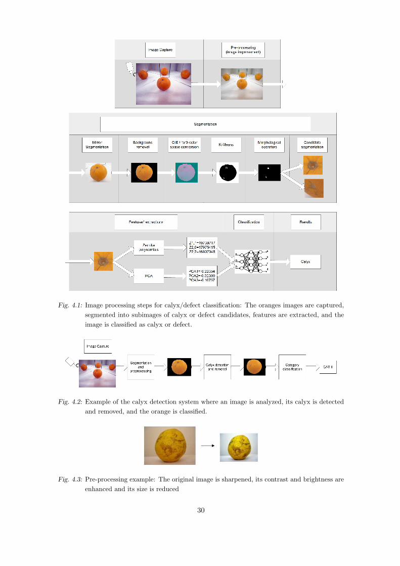
Fig. 4.1: Image processing steps for calyx/defect classification: The oranges images are captured,
segmented into subimages of calyx or defect candidates, features are extracted, and the
image is classified as calyx or defect.
Fig. 4.2: Example of the calyx detection system where an image is analyzed, its calyx is detected
and removed, and the orange is classified.
Fig. 4.3: Pre-processing example: The original image is sharpened, its contrast and brightness are
enhanced and its size is reduced
30

Background removal: Being Io and Ib the regions for the orange (foreground) and
background, we extract the region Io from the background by first improving the contrast
of the image I and extracting the blue component from the RGB color space.
The choice of the blue component is because it is the component that most discrimi-
nates the background of the image, due to the fact that for the orange color (made of red
and some green), the value of the blue component is zero. This can be seen in Figure 4.4.
(a) Component R (b) Component G (c) Component B (d) RGB with 1 pixel
Fig. 4.4: Red, Green and Blue (RGB) components of an image.
The gray-level image obtained is then converted to black and white followed by mor-
phological operations (erosion and dilation) for noise reduction [49]. After obtaining a
binary image, a contour tracking algorithm is used to detect the border of the orange in
the original color image to extract the background [49].
This process is done for every image captured.
Mirror segmentation: When using mirrors in the capture step, it is necessary to
identify the different sections of the image where an orange is found. The process is similar
to the background removal: first we improve the contrast of the image and extract the blue
component. Next, the image is binarized, morphological operators are applied following
by a contour tracking algorithm. An example of the original image with the contours of
the orange highlighted is shown in Figure 4.5.
Fig. 4.5: Mirror segmentation
31

Calyx candidate regions extraction:
• CIE L*a*b* Color space conversion: The first step is to convert the image
with the background removed to the CIE L*a*b* color space. As it was previously
explained in section 2.1.2, the CIE L*a*b* color space is considered as one of the
best color spaces for matching the human perception distance of colors [14]. This
is because the difference between two colors can be related to the perceptual dis-
tance [14] and thus it is a useful color space to perform cluster analysis. The color
space consists of three layers. The Luminance or brightness layer L∗, the Red-Green
chromatic layer a∗ and the Blue-Yellow chromatic layer b∗ [26].
Once the color space conversion is done, we discard the L∗ component (because it
does not contain color information), and perform a non supervised cluster analysis
to detect different regions.
• K-Means cluster analysis: Cluster analysis is the process of grouping similar
objects into the same class [16]. The similarity of two objects is determined by
measuring the distance between them, which can be calculated in different ways, like
Euclidean distance, normalized Euclidean distance, Mahalanobis distance, etc. [12].
In this thesis we use k-means clustering with Euclidean distance and the number of
clusters chosen is k=2, aiming to find two regions: one for the healthy skin and other
for the calyx or defect. The distinction between calyxes and defects is performed in
a further step.
The result of the k-means process is a binary image with two regions: The region of
healthy skin and the region of the calyx or defect. However, as the image obtained can be
noisy, morphological operators are applied. A scheme of this process is shown in Figure 4.6.
It is performed for every image captured obtaining a total of nc calyx candidate images.
As the aim of this process is to identify the region where a calyx could be found, and
we know the average diameter of the calyx in an image, we discard the candidate regions
which have a diameter smaller than the average (about 5 pixels in 192x144 pixel images).
Fig. 4.6: K-Means clustering after performing CIE L*a*b* colorspace conversion
32

4.3 Feature extraction
Once the image is segmented, it is necessary to obtain several features in order to be able
to perform the classification.
The objects in the image can be characterized by different descriptors like gray levels,
color, texture, gradient, second derivative and by geometrical properties like area, perime-
ter, Fourier descriptors and invariant moments [43, 9]. For instance, Unay & Gosselin [10]
extract the background, stem, good peel and defective peel for classifying oranges.
In this section, the features obtained are a series of Zernike moments and the first ten
Principal Components.
We choose Zernike moments for calyx detection because they are rotation invariant [1],
which makes them suitable for analyzing symmetrical objects like calyxes. Zernike mo-
ments are very useful in image processing and recognition, and are widely used in face
detection applications, like in [29], where authors perform eye detection using Zernike
Moments and use a Support Vector Machine for classification.
In [5], a face recognition system for video surveillance is presented, where they perform
a comparison between Zernike moments, Eigenfaces (Principal Component Analysis) and
Fisherfaces.
Other image processing applications which use Zernike polynomials include a system
presented by [39] which uses Zernike polynomials to model the global shape of the cornea,
and use a decision tree classifier which takes as features the polynomial coefficients.
Other reason for trying Zernike polynomials are the good results obtained by Recce
et. al [37] for stem-end/calyx detection in oranges. We also choose to use Principal
Component Analysis as they are widely used in image processing tasks like face recognition
(eigenfaces) [7], and also for stem end/calyx detection in apples [20].
33

4.3.1 Zernike Moments
Zernike Moments moments are very useful in image processing and recognition because
they are rotation invariant and form a complete orthogonal set over the interior of the
unitary circle [1]. The projection of the image over these sets are the Zernike moments [2].
The form of the polynomials is denoted by
Znm(x, y) = Znm(ρ, σ) = Rnm(ρ)e(jmθ), (4.1)
where j =√−1, ρ is the length from origin (0, 0) to (x, y), and θ the angle between the
x axis and the vector from origin to (x, y) in a counter clockwise direction, n ∈ N0 is the
order of the polynomial, and m ∈ Z is the rotation degree [3].
The restriction: n − |m| is even and |m| < n [1] has to be satisfied.
Rnm(ρ) is the radial polynomial defined by
Rnm(ρ) =
(n−|m|)/2∑
s=0
(−1)s(n − s)!ρn−2s
s!(n+|m|2 − s)!(n−|m|
2 − s)!(4.2)
and according to Euler’s formula: e(jmθ) = cos(mθ) + jsin(mθ).
The Zernike moment Amn for a continuous function f(x, y) is defined as
Anm =n + 1
π
∫ ∫
x2+y2≤1f(x, y)Z∗
nm(ρ, θ)dxdy (4.3)
and for a digital image of size M × N as
Anm =n + 1
π
M∑
x=1
N∑
y=1
f(x, y)Z∗nm(ρ, θ) (4.4)
where [∗] denotes the complex conjugate [4]. Anm can also be seen as the multiplication of
the original image f(x, y) with a mask. Each component of the image Anm is a complex
value. In Figure 4.7 an image of a Zernike mask of order Z5,1 is shown.
For every image from the previous step, we compute the Zernike moments from order
n=1 to order n=12, so we obtain 48 Zernike-images. The first 12 Zernike Moments and
their dimensions are shown in Table 4.1. For each one we calculate the sum of the absolute
values of each pixel and these values are used in the classification step.
34

(a) Z5,1 Real (b) Z5,1 Imaginary
Fig. 4.7: Zernike moment masks examples for n=5, m=1
Order n Dimension Zernike Moments
0 1 Z0,0
1 2 Z1,1
2 4 Z2,0 Z2,2
3 6 Z3,1 Z3,3
4 9 Z4,0 Z4,2 Z4,4
5 12 Z5,1 Z5,3 Z5,5
6 16 Z6,0 Z6,2 Z6,4 Z6,6
7 20 Z7,1 Z7,3 Z7,5 Z7,7
8 25 Z8,0 Z8,2 Z8,4 Z8,6 Z8,8
9 20 Z9,1 Z9,3 Z9,5 Z9,7 Z9,9
10 26 Z10,0 Z10,2 Z10,4 Z10,6 Z10,8 Z10,10
11 42 Z11,1 Z11,3 Z11,5 Z11,7 Z11,9 Z11,11
12 49 Z12,0 Z12,2 Z12,4 Z12,6 Z12,8 Z12,10 Z12,12
Tab. 4.1: First 12 Zernike Moments
4.3.2 Principal Component Analysis (PCA)
PCA is a procedure used in multivariate data analysis which performs an orthogonal linear
transformation to a set of correlated variables into a set of non correlated variables called
principal components (PC) [12]. One of the main purposes of this procedure is to obtain a
dimensionality reduction. Principal Component Analysis is used in several applications in
image processing, specially with large datasets or very large images like satellite images.
The projection of the variables into the new coordinate system is also called the
Karhunen-Loeve transform (KLT) or Hotelling transform [7].
When this method is applied to a set of correlated variables in a space of dimension
D, the transformation diagonalizes the covariance matrix and creates a new coordinate
35

system. These coordinates are the Principal Components and they are sorted by decreasing
variance. This means that low order components explain the highest variance of the data,
and by keeping the P first components, most of the variability is retained, leading to a
dimensionality reduction (P << D) [12, 7].
The criterion used in this thesis for deciding how many components P are enough to
explain most of the variance, are the following:
1. The first criterion consists of adding the explained variance for each Principal Com-
ponent until the accumulated explained variance is higher than a certain threshold
(e.g. 80% of the total variance) [12]. Figure 4.8 (a) shows an example of this plot.
2. The second criterion is based on a SCREE plot of eigenvalues. The point in which
the curve tends to stabilize is the number of components required. An example is
shown in Figure 4.8 (b). In this example, the number of components to be chosen
should be five, since in that component the curve tends to stabilize.
3. The third criterion, which is valid only for PCA analysis using the correlation matrix,
consists of keeping the eigenvalues greater than 1, so the dimension of the space is
equal to the number of eigenvalues greater than 1.
The first two criteria can be applied when using both the variance-covariance matrix
and the correlation matrix, and the third can only be applied when using the correlation
matrix [12].
(a) Pareto plot which shows the percentage of
variance explained.
0 2 4 6 8 10 120
0.5
1
1.5
2
2.5
3
3.5
4
Eigenvalue number
Eig
enva
lue
(b) SCREE plot.
Fig. 4.8: PCA evaluation criteria.
In this thesis, we perform the Principal Components Analysis in the following way:
for every calyx candidate image Icc of size M × N obtained in the segmentation step, we
first convert from RGB to HSV to obtain the hue component and then convert the image
matrix to a vector of size 1×M ×N , obtaining a dataset of size nc ×M ×N of real values
ranging from 0 to 1, being nc the number of calyx candidate images of the dataset.
36

The choice of the H component was done empirically comparing the results of perform-
ing PCA using R, G, B, H, S, V , and gray level components. These results are shown in
Figures 4.9 (a) and (b), where it can be seen that while the variance explained by the first
principal component is higher when using the Red and Saturation components compared
to the variance explained by the first component of the Hue component, the eigenvalues
of the second and third principal components of H are much higher than in the others,
thus the accumulated variance explained of H is higher than in the rest.
(a) SCREE plot
(b) Accumulated SCREE plot
Fig. 4.9: SCREE plots showing the variance explained by performing PCA over each component
of the RGB and HSV color spaces
As all the variables are in the same unit and within the same range, we perform the
Principal Component Analysis over the covariance matrix, without needing to standardize
the data [12]. The results of the PCA are the coefficients of the linear transformation
(Cpca), which are used to obtain the projected images (Pij) in the new coordinate system.
37

In [12], the number of components P needed in the classification step is P=3 or P=4.
If we consider the SCREE plot, the number of components when the curve stabilizes is
around P=5. However, in order to compare the performance of the classifiers using many
different number of PCs, we keep the first ten principal components to use them in the
classification step.
An example of the values of the first two components for classifying calyxes or defects
is shown as a scatter plot in Figure 4.10.
Fig. 4.10: Scatter plot of the first two principal components for calyx and defect detection
Once the features of the Zernike moments and Principal Components are extracted, a
consolidated dataset is built. It contains nc rows (one for each calyx candidate), and 58
columns (48 from the Zernike moments and 10 from the first PCs). Also the class was
added to the dataset in order to use supervised learning algorithms.
38
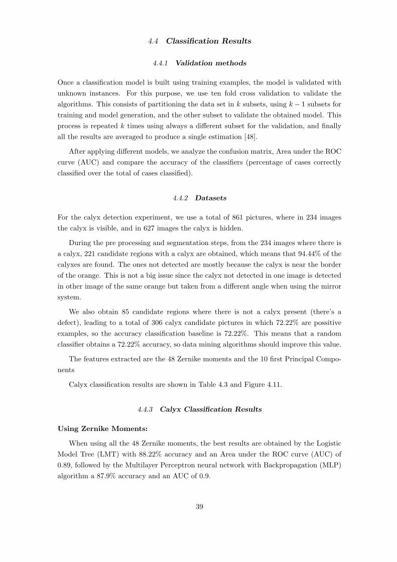
4.4 Classification Results
4.4.1 Validation methods
Once a classification model is built using training examples, the model is validated with
unknown instances. For this purpose, we use ten fold cross validation to validate the
algorithms. This consists of partitioning the data set in k subsets, using k − 1 subsets for
training and model generation, and the other subset to validate the obtained model. This
process is repeated k times using always a different subset for the validation, and finally
all the results are averaged to produce a single estimation [48].
After applying different models, we analyze the confusion matrix, Area under the ROC
curve (AUC) and compare the accuracy of the classifiers (percentage of cases correctly
classified over the total of cases classified).
4.4.2 Datasets
For the calyx detection experiment, we use a total of 861 pictures, where in 234 images
the calyx is visible, and in 627 images the calyx is hidden.
During the pre processing and segmentation steps, from the 234 images where there is
a calyx, 221 candidate regions with a calyx are obtained, which means that 94.44% of the
calyxes are found. The ones not detected are mostly because the calyx is near the border
of the orange. This is not a big issue since the calyx not detected in one image is detected
in other image of the same orange but taken from a different angle when using the mirror
system.
We also obtain 85 candidate regions where there is not a calyx present (there’s a
defect), leading to a total of 306 calyx candidate pictures in which 72.22% are possitive
examples, so the accuracy classification baseline is 72.22%. This means that a random
classifier obtains a 72.22% accuracy, so data mining algorithms should improve this value.
The features extracted are the 48 Zernike moments and the 10 first Principal Compo-
nents
Calyx classification results are shown in Table 4.3 and Figure 4.11.
4.4.3 Calyx Classification Results
Using Zernike Moments:
When using all the 48 Zernike moments, the best results are obtained by the Logistic
Model Tree (LMT) with 88.22% accuracy and an Area under the ROC curve (AUC) of
0.89, followed by the Multilayer Perceptron neural network with Backpropagation (MLP)
algorithm a 87.9% accuracy and an AUC of 0.9.
39

However, when using only the first 5 moments, the Multilayer perceptron increases
its accuracy to 88.88% and AUC to 0.91, and the Logistic model tree achieves 88.66%
accuracy with an AUC of 0.91.
Also, good results are obtained when using only the first 3 Zernike moments: the
Multilayer perceptron achieves an accuracy of 88.87% and an AUC of 0.91 while the
Logistic Model Tree has an accuracy of 88.12% and an AUC of 0.91.
We perform Chi Squared Attribute Evaluation with Ranker, and pick-up the first 20
attributes to perform the classifier’s comparison. The results obtained are worse than
using all the 48 Zernike moments: MLP and LMT achieve an accuracy near 84% and an
AUC near 0.9, while SMO and RBF Network equal the baseline accuracy of 72.24%.
Using Principal Component Analysis (PCA): The best accuracy is obtained
when using only the first 10 principal components, and is achieved by the Radial Basis
Function Network with 81.05% accuracy and an AUC of 0.84. The same algorithm obtains
an accuracy of 80.82% and an AUC of 0.86 when using only the first three principal
components.
Combining Zernike Moments and Principal Component Analysis: We per-
form several combinations of Zernike moments and principal components. The best results
are obtained with the Logistic Model tree when combining the first 5 Zernike moments
with the first two principal components, obtaining an accuracy of 89.87% and an AUC of
0.93.
We also obtained similar results with the Multilayer Perceptron Neural Network when
combing the first 5 Zernike moments with the first principal component, achieving an
accuracy of 88.89% and an AUC of 0.92.
The confusion matrix of these classifiers are shown in Table 4.2
Algorithm
``
``
``
``
``
``
``
``
True class
Predicted classCalyx Defect Accuracy AUC
Zernike 5, PCA 2 Calyx 213 889.87% 0.93
LMT Defect 23 62
Zernike 5, PCA 1 Calyx 209 1288.89% 0.92
MLP Defect 22 63
Tab. 4.2: Calyx classification confusion matrices
40
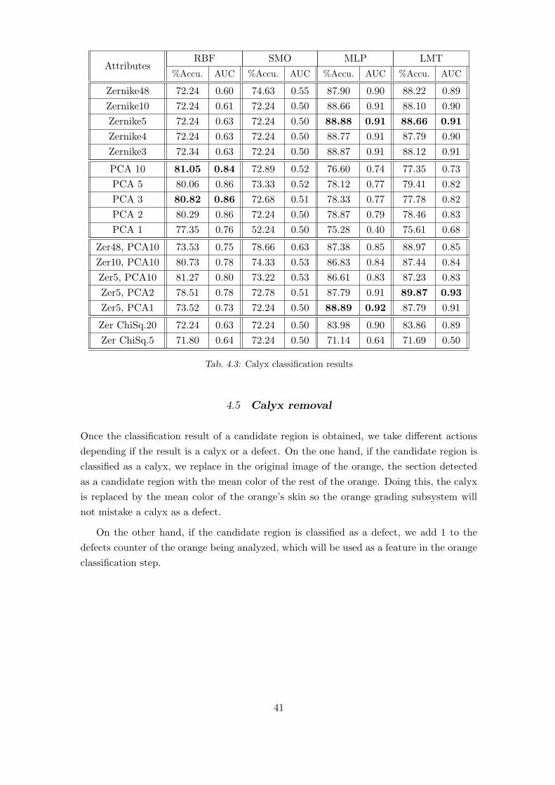
AttributesRBF SMO MLP LMT
%Accu. AUC %Accu. AUC %Accu. AUC %Accu. AUC
Zernike48 72.24 0.60 74.63 0.55 87.90 0.90 88.22 0.89
Zernike10 72.24 0.61 72.24 0.50 88.66 0.91 88.10 0.90
Zernike5 72.24 0.63 72.24 0.50 88.88 0.91 88.66 0.91
Zernike4 72.24 0.63 72.24 0.50 88.77 0.91 87.79 0.90
Zernike3 72.34 0.63 72.24 0.50 88.87 0.91 88.12 0.91
PCA 10 81.05 0.84 72.89 0.52 76.60 0.74 77.35 0.73
PCA 5 80.06 0.86 73.33 0.52 78.12 0.77 79.41 0.82
PCA 3 80.82 0.86 72.68 0.51 78.33 0.77 77.78 0.82
PCA 2 80.29 0.86 72.24 0.50 78.87 0.79 78.46 0.83
PCA 1 77.35 0.76 52.24 0.50 75.28 0.40 75.61 0.68
Zer48, PCA10 73.53 0.75 78.66 0.63 87.38 0.85 88.97 0.85
Zer10, PCA10 80.73 0.78 74.33 0.53 86.83 0.84 87.44 0.84
Zer5, PCA10 81.27 0.80 73.22 0.53 86.61 0.83 87.23 0.83
Zer5, PCA2 78.51 0.78 72.78 0.51 87.79 0.91 89.87 0.93
Zer5, PCA1 73.52 0.73 72.24 0.50 88.89 0.92 87.79 0.91
Zer ChiSq.20 72.24 0.63 72.24 0.50 83.98 0.90 83.86 0.89
Zer ChiSq.5 71.80 0.64 72.24 0.50 71.14 0.64 71.69 0.50
Tab. 4.3: Calyx classification results
4.5 Calyx removal
Once the classification result of a candidate region is obtained, we take different actions
depending if the result is a calyx or a defect. On the one hand, if the candidate region is
classified as a calyx, we replace in the original image of the orange, the section detected
as a candidate region with the mean color of the rest of the orange. Doing this, the calyx
is replaced by the mean color of the orange’s skin so the orange grading subsystem will
not mistake a calyx as a defect.
On the other hand, if the candidate region is classified as a defect, we add 1 to the
defects counter of the orange being analyzed, which will be used as a feature in the orange
classification step.
41

Fig. 4.11: Comparison of classifiers accuracy among the different attributes selection.
4.6 Conclusions
As an essential part of the fruit grading system, the stem-end/calyx detection subsystem
is the responsible for distinguishing a calyx from a defect.
After acquiring the image, it is necessary to improve the quality of the picture and
identify the regions of interest (ROI) by removing the background and identifying the
regions where the different views of the orange are present when using the mirror capture
system.
Then, we segment the images into calyx candidate regions using k-means clustering
over the CIE L*a*b* color space, and once we have all the candidate regions, we use
Zernike polynomials and perform Principal Component Analysis to extract the features
to be used in the calyx classification step.
Although the amount of descriptors retrieved might seem excessive, the data mining
algorithms should discard the less significant attributes, and we also experiment using fea-
tures subset selection algorithms in order to keep only the most significant attributes and
compare the classification results using different datasets containing different combinations
of features.
42

After the dataset is built, we perform the classification of candidate regions as calyxes
or defects, using machine learning algorithms like Logistic Model Tree, Multilayer percep-
tron network with backpropagation, Sequential minimal optimization for support vector
machine and Radial basis function network.
The results of the experiments show that both Logistic Model Tree and Multilayer
Perceptron neural network achieve very good accuracy (89.87% for LMT and 88.89% for
MLP) and a very good AUC value (0.93 for LMT and 0.92 for MLP) when processing
datasets with the first 5 Zernike moments and the first two and one principal components
respectivly.
The Radial Basis Function Network achieves the highest accuracy (81.05%) when pro-
cessing a dataset with only principal components. However, its performance decreases
significantly when using a dataset which contains only Zernike moments.
SMO shows very poor results, with a maximum accuracy of only 78.66% achieved when
using the dataset with the 48 Zernike moments and the first 10 principal components.
The comparison of all the classifiers analyzed using the different data sets are shown
in Table 4.3 and Figure 4.11.
Based on the obtained results, the chosen classifier for us would be the Logistic Model
Tree, because of its high accuracy across the different attributes configuration, and also
because of the easier interpretation of the model compared to neural networks. According
to the bibliography, one of the disadvantages of this classifier is the high computational cost
for real time applications [42], that is not analyzed in this thesis but should be considered
in a future work because of the real time requirements of fruit grading production lines.
The obtained accuracy (89.87%) can be compared to results of similar researches per-
formed by other authors. Unay and Gosselin [10] classify apple’s calyx/stem-end with 81%
accuracy when using a KNN classifier and 90.5% accuracy using SV M . Ruiz et. al [34]
achieve 93% accuracy when classifying stem, calyx and leaves against skin and background
in oranges using Bayesian decision rules.
43

5. QUALITY CATEGORIES CLASSIFICATION
The quality classification subsystem is one of the main parts of the orange grading system.
Its input is the output of the calyx detection subsystem, consisting of the original image
captured by the image capture subsystem, already pre-processed and mirror segmented
and with the calyx removed. The purpose of this step is to process the image in order to
describe that picture as a series of features that are used by the data mining algorithms in
the classification step to classify the orange into one of the three pre-established categories.
This chapter is one of the most relevant parts of this thesis.
A diagram of the Input-Process-Output is shown in Figure 5.1, which shows that the
input to the classification algorithms is a dataset containing the features extracted, and
the output of the process is the classification result.
Fig. 5.1: Input-Process-Output diagram of the system where features are extracted, processed and
classified
The quality categories classification subsystem is further divided into the following
steps:
• Feature extraction
• Classification

Pre-processing and segmentation tasks have already been described in section 4.1 and
no further pre-processing or segmentation is needed at this step.
A diagram of this process can be seen in Figure 5.2.
Fig. 5.2: Image processing steps.
5.1 Feature extraction
In this section, the features obtained are the area of the orange and the background, the
fractal dimension of region Io, the contrast, gray level uniformity, gray level correlation
between neighbours, histogram, and the mean and median calculated in the HSV color
space.
The data mining algorithms used in the classification step should automatically detect
the most relevant attributes (features) needed to perform the classification, discarding the
rest. Therefore, in the feature extraction step we gather as many descriptors as we can in
order to make classification algorithms more effective.
Next we explain in detail each one of the features extracted.
• Orange area: The area of the orange Ao is calculated as the sum of the pixels be-
longing to the orange: Ao =∑144
i=1
∑192j=1 f(i, j), where f(i, j) =
{
1 if (i, j) ∈ In
0 in other case
We also calculate the complement descriptor (background area) Ab.
• Fractal dimension analysis:
The fractal dimension FD of a set in Rn, is a real number which characterizes its
geometrical complexity, and can be used as an irregularity indicator of a set [27, 54].
The FD is defined for self-similar sets, and in the case of sets which do not have this
property, the FD has to be estimated [57].
One of the methods proposed in [27] to estimate FD and characterize the smooth-
ness level in a section of an image is the box-counting dimension. This method is
commonly used because it exhibits a good balance between computation time and
45
accuracy. However, this estimation has the inconvenient that can only be applied to
binary images.
The box-counting dimension of a planar set A consists of estimating how changes
the quantity of cells in which the set has no null measure, as function of the size of
those cells.
Being Nl(A) the quantity of cells of side l where the set has no null measure, the
box-counting dimension DB of A is
DB = liml→0
log(Nl(A))
log(1l )
, (5.1)
if the limit exists. In practice, for finite resolution images, l has superior and inferior
limits, and DB can be estimated with the slope of the minimum square regression
that approximates the logarithmic diagram log(Nl(A))vs. log(1l ).
Given a binary image, it is partitioned in cells of side l, and for different values of l,
the quantity Nl(A) of cells in which the object of interest (foreground) has no null
measure is calculated. Except the case in which l = 1, for all l, it is necessary to
make many partitions of the image and calculate Nl(A) as the average. Then, DB
is estimated as the minimum square regression slope previously mentioned.
To be able to apply this method it is necessary to transform the image to binary, so
a thresholding process has to be applied for this purpose. In this thesis, in order to
obtain the texture of the peel of the fruit to estimate the fractal dimension, we start
from a gray level image of the orange with the background removed, and apply a
border detection procedure with the Canny [13] algorithm, getting the image Ican.
Then, the box counting dimension DB is calculated over the image Ican. A result
of 1 means that the texture of the orange’s peel is smooth, which means that it is
a good quality orange. In the opposite side, for greater imperfections, the value of
the estimator DB tends to increase.
Table 5.1 shows the results of the border detection with the Canny algorithm, and
the fractal dimension obtained for a good quality orange and a defective quality one,
where it can be seen that the value of DB in the good orange is lower (tending to
1) than in the defective one.
• Texture analysis using statistical descriptors: For the texture analysis we use
six statistical descriptors, which use a co-occurrences gray level matrix. This is made
calculating the number of adjacent pixel repetitions with the same gray level in the
whole image.
The statistical descriptors used are:
– Contrast: The global contrast of the image (also known as variance or in-
ertia) measures the contrast intensity between a pixel and its neighbour. Its
calculation is based on the corresponding co-occurrences matrix.
46

Good orange Defective orange
Original image
Border detection
Fractal Dimension 1.0887 1.2688
Tab. 5.1: Steps in the estimation of the fractal dimension
– Correlation: Measures the relation of a pixel and its neighbour. The degree
in which if the gray level of a pixel increases, its neighbour also increases.
– Energy: Also known as ’uniformity’, ’energy uniformity’ and ’second angular
moment’, consists of the sum of the squared elements in the co-occurrences
matrix taken by pairs.
– Homogeneity: It is a value that measures the closeness of the distribution of
elements of the co-occurrences matrix to the main diagonal of that matrix.
– Skewness: It is a measure of the degree of asymmetry of a distribution around
the mean. It is obtained by calculating the third standardized central moment
of the distribution. If the obtained value is zero, it means that it is centered
(like the normal distribution). If it is positive, it is asymmetrical to the right,
and if it is negative, to the left [22].
– Kurtosis: Measures how distant is the distribution of the data to the normal
distribution. Is the result of calculating the fourth standardized central moment
of a distribution. The kurtosis of the normal distribution is 3. A value greater
than 3 (platykurtic) means that the distribution is flatter (with thicker tails),
and a distribution with kurtosis less than 3 (leptokurtic) means the opposite
(thiner tails and a sharp peak) [22].
A comparison of the values of these statistical descriptors of a good and defective
orange are shown in Table 5.2
• Histograms analysis: We analyze the histograms of the red Hr, green Hg, blue
Hb, and the gray levels Hgray histograms. A RGB histogram example can be seen
in Figure 5.3. To simplify the analysis, we divide the histograms in six bins. For
example, for the red component, the first bin is the amount of pixels in the image
which values belong to the interval [0, 2556 ), the second bin [2556 , 255
6 × 2) and so on
until the six intervals are covered.
47
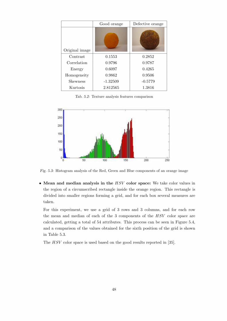
Good orange Defective orange
Original image
Contrast 0.1553 0.2852
Correlation 0.9796 0.9787
Energy 0.6097 0.4265
Homogeneity 0.9862 0.9506
Skewness -1.32509 -0.5779
Kurtosis 2.812565 1.3816
Tab. 5.2: Texture analysis features comparison
Fig. 5.3: Histogram analysis of the Red, Green and Blue components of an orange image
• Mean and median analysis in the HSV color space: We take color values in
the region of a circumscribed rectangle inside the orange region. This rectangle is
divided into smaller regions forming a grid, and for each box several measures are
taken.
For this experiment, we use a grid of 3 rows and 3 columns, and for each row
the mean and median of each of the 3 components of the HSV color space are
calculated, getting a total of 54 attributes. This process can be seen in Figure 5.4,
and a comparison of the values obtained for the sixth position of the grid is shown
in Table 5.3.
The HSV color space is used based on the good results reported in [35].
48

Fig. 5.4: Region of the image used to extract the mean and median features of the HSV color
space.
Good orange Defective orange
Original image
Hue Mean 0.0349 0.0622
Saturation Mean 0.4982 0.7904
Value Mean 0.8044 0.3713
Hue Median 0.0590 0.0572
Saturation Median 0.9434 0.7931
Value Median 0.6588 0.3529
Tab. 5.3: HSV mean and median features comparison. Hue ranges from 0 (0o=red) to 1 (360o),
saturation ranges from 0 (unsaturated) to 1 (fully saturated), and value ranges from 0
(black) to 1 (brightest)
5.2 Classification Results
For this experiment we use a data set obtained after processing a total of 892 oranges’
images, which contains 314 high quality oranges’ images, 473 intermediate quality oranges’
images and 105 defective quality oranges’ images. For each specimen, we extract the 95
previously described features, which are all numerical attributes. The class assignment
was done manually by the authors, based on visual features and on expert’s advise.
When analyzing the results, we perform a cost sensitive evaluation, since the cost of
misclassifying a defective orange as a good orange is much higher than misclassifying a
good orange as defective, because if a good orange is classified as defective, the revenue
obtained by selling the fruit as a lower category will be lower than selling it as a good one.
However, if a defective orange is sold as good, it is sold at a higher price, but when the
buyer finds out that defective oranges have been sold as good, he can demand the seller
to pay a fine and he will likely not buy anymore products.
The cost-matrix used is shown in Table 5.4.
49

``
``
``
``
``
``
``
``
True class
Predicted classGood Intermediate Defective
Good 0 1 2
Intermediate 2 0 1
Defective 5 2 0
Tab. 5.4: Cost-Matrix
• Results obtained with a J48 decision tree: After training a J48 decision tree
with the described dataset, the decision tree shown in Figures 5.7 a) and 5.5 is
generated. It can be seen that the attribute fractalDim (the fractal dimension) is
in the root of the tree. This means that this is the best attribute to differentiate
between classes.
Fig. 5.5: J48 Decision tree
As it can be seen in the confusion matrix shown in Table 5.6, the accuracy achieved
by the classifier is 71.08%. From all of the classification errors we obtain, there are
4 good oranges misclassified as defective, and 2 defective oranges misclassified as
good. The rest of the misclassifications are between the ’intermediate’ class and the
others, thus the cost is 420.
We also trained a decision tree with the same configuration but using only two
classes (’good’ and ’defective’) from the original dataset. The obtained decision tree
is shown in Figure 5.6, where it can be seen that it contains the fractal dimension
attribute as root node. This classifier achieves a 94.75% accuracy and an area under
the ROC curve of 0.93, as it can be seen in the confusion matrix shown in Table 5.5.
50

Fig. 5.6: J48 decision tree for only two classes: ’good’ and ’defective’.
• Results obtained with a Best First decision tree: Figure 5.7 b) shows the
model generated by the Best First algorithm. In the root node it has the third bin
of the red histogram, and other discriminant attributes are the histograms of the
green and gray components of the RGB color space and the fractal dimension. The
accuracy of this model is 72.20% and the total cost is 398 (see Table 5.6).
• Results obtained with a Logistic Model Tree (LMT ): The model built with
the LMT algorithm achieves an accuracy of 81.73%, and as it can be seen in the
confusion matrix shown in Table 5.6, it does not commit any classification mistake
between ’good’ and ’defective’ classes. Thus, with its cost being the lowest one with
252, it is the best model obtained for classifying oranges in three classes.
• Results obtained with a Random Forest decision tree: The accuracy obtained
with this tree is 73.54%. Analyzing the confusion matrix, we notice that there is
only one error between the ’good’ and ’defective’ classes, but there are many errors
between the ’intermediate’ and other classes, having a cost of 368.
• Results obtained with a Simple CART decision tree: This decision tree
achieves an accuracy of 72.76% and a cost of 383 (see Table 5.6), creating a model
similar to the one obtained with the Best First algorithm (see Figure 5.7 b)), as
it has the third bin of the red histogram as the root element, and has the fractal
dimension and the histograms of the green and gray components of the RGB color
space among other discriminant attributes.
51

a) J48
fractalDim <= 1.190237
| red3 <= 123
| | correlationH <= 0.975922: intermed (20.0/7.0)
| | correlationH > 0.975922
| | | gray6 <= 1220
| | | | green1 <= 2: good (42.0)
| | | | green1 > 2
| | | | | skewnessGray <= -2.183524
| | | | | | DBC128_191 <= 2.104028: good (17.0/3.0)
| | | | | | DBC128_191 > 2.104028: intermed (16.0)
| | | | | skewnessGray > -2.183524
| | | | | | fractalDim <= 1.119564: good (95.0/4.0)
| | | | | | fractalDim > 1.119564
| | | | | | | gray5 <= 408
| | | | | | | | VMean9 <= 0.099359: good (15.0/5.0)
| | | | | | | | VMean9 > 0.099359: intermed (16.0/1.0)
| | | | | | | gray5 > 408: good (68.0/12.0)
| | | gray6 > 1220: intermed (20.0/6.0)
| red3 > 123
| | correlation <= 0.973437: intermed (69.0/25.0)
| | correlation > 0.973437
| | | gray3 <= 16
| | | | green5 <= 1512: intermed (26.0/5.0)
| | | | green5 > 1512
| | | | | DBC <= 1.95728
| | | | | | Hmean7 <= 0.092857: good (17.0/5.0)
| | | | | | Hmean7 > 0.092857: intermed (25.0)
| | | | | DBC > 1.95728
| | | | | | fractalDim <= 1.114206: good (33.0/6.0)
| | | | | | fractalDim > 1.114206: intermed (28.0/12.0)
| | | gray3 > 16
| | | | Hmean6 <= 0.074675
| | | | | green5 <= 4227: intermed (18.0/5.0)
| | | | | green5 > 4227: good (15.0/3.0)
| | | | Hmean6 > 0.074675: intermed (212.0/10.0)
fractalDim > 1.190237
| red3 <= 148: good (15.0/7.0)
| red3 > 148
| | contrast <= 0.164776
| | | DBC192_255 <= 2.046449: deffecti (30.0/8.0)
| | | DBC192_255 > 2.046449
| | | | DBC0_63 <= 2.00646: deffecti (29.0/13.0)
| | | | DBC0_63 > 2.00646: intermed (36.0/6.0)
| | contrast > 0.164776: deffecti (30.0/1.0)
52

b) BFTree
red3 < 131.0
| green5 < 1042.5
| | red3 < 16.0: good(47.0/12.0)
| | red3 >= 16.0: intermed(43.0/27.0)
| green5 >= 1042.5: good(167.0/33.0)
red3 >= 131.0
| fractalDim < 1.19042
| | gray3 < 23.5
| | | green5 < 1695.5: intermed(50.0/19.0)
| | | green5 >= 1695.5
| | | | DBC < 1.96616
| | | | | VMean7 < 0.09423: good(12.0/5.0)
| | | | | VMean7 >= 0.09423: intermed(29.0/2.0)
| | | | DBC >= 1.96616: good(39.0/25.0)
| | gray3 >= 23.5
| | | Hmean5 < 0.07167: good(16.0/15.0)
| | | Hmean5 >= 0.07167: intermed(208.0/16.0)
| fractalDim >= 1.19042
| | gray5 < 2.5
| | | fractalDim < 1.20863: deffecti(6.0/4.0)
| | | fractalDim >= 1.20863: deffecti(30.0/0.0)
| | gray5 >= 2.5
| | | fractalDim < 1.25802
| | | | DBC < 1.9595: deffecti(15.0/6.0)
| | | | DBC >= 1.9595
| | | | | fractalDim < 1.20052: deffecti(6.0/5.0)
| | | | | fractalDim >= 1.20052
| | | | | | Hmean5 < 0.10536: intermed(8.0/5.0)
| | | | | | Hmean5 >= 0.10536: intermed(30.0/1.0)
| | | fractalDim >= 1.25802: deffecti(10.0/1.0)
c) Simple CART
red3 < 131.0
| green5 < 1042.5
| | red3 < 16.0: good(47.0/12.0)
| | red3 >= 16.0: intermed(43.0/27.0)
| green5 >= 1042.5: good(167.0/33.0)
red3 >= 131.0
| fractalDim < 1.19042: intermed(332.0/104.0)
| fractalDim >= 1.19042
| | gray5 < 2.5: deffecti(36.0/4.0)
| | gray5 >= 2.5
| | | fractalDim < 1.25802
| | | | DBC < 1.9595: deffecti(15.0/6.0)
| | | | DBC >= 1.9595: intermed(42.0/13.0)
| | | fractalDim >= 1.25802: deffecti(10.0/1.0)
Fig. 5.7: Decision trees and classification rule models.
53
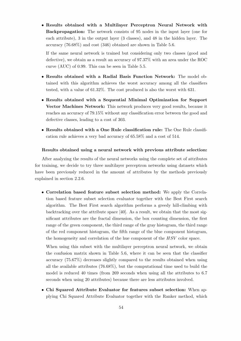
• Results obtained with a Multilayer Perceptron Neural Network with
Backpropagation: The network consists of 95 nodes in the input layer (one for
each attribute), 3 in the output layer (3 classes), and 48 in the hidden layer. The
accuracy (76.68%) and cost (346) obtained are shown in Table 5.6.
If the same neural network is trained but considering only two classes (good and
defective), we obtain as a result an accuracy of 97.37% with an area under the ROC
curve (AUC) of 0.99. This can be seen in Table 5.5.
• Results obtained with a Radial Basis Function Network: The model ob-
tained with this algorithm achieves the worst accuracy among all the classifiers
tested, with a value of 61.32%. The cost produced is also the worst with 631.
• Results obtained with a Sequential Minimal Optimization for Support
Vector Machines Network: This network produces very good results, because it
reaches an accuracy of 79.15% without any classification error between the good and
defective classes, leading to a cost of 303.
• Results obtained with a One Rule classification rule: The One Rule classifi-
cation rule achieves a very bad accuracy of 65.58% and a cost of 514.
Results obtained using a neural network with previous attribute selection:
After analyzing the results of the neural networks using the complete set of attributes
for training, we decide to try three multilayer perceptron networks using datasets which
have been previously reduced in the amount of attributes by the methods previously
explained in section 2.2.6.
• Correlation based feature subset selection method: We apply the Correla-
tion based feature subset selection evaluator together with the Best First search
algorithm. The Best First search algorithm performs a greedy hill-climbing with
backtracking over the attribute space [40]. As a result, we obtain that the most sig-
nificant attributes are the fractal dimension, the box counting dimension, the first
range of the green component, the third range of the gray histogram, the third range
of the red component histogram, the fifth range of the blue component histogram,
the homogeneity and correlation of the hue component of the HSV color space.
When using this subset with the multilayer perceptron neural network, we obtain
the confusion matrix shown in Table 5.6, where it can be seen that the classifier
accuracy (75.67%) decreases slightly compared to the results obtained when using
all the available attributes (76.68%), but the computational time used to build the
model is reduced 40 times (from 269 seconds when using all the attributes to 6.7
seconds when using 20 attributes) because there are less attributes involved.
• Chi Squared Attribute Evaluator for features subset selection: When ap-
plying Chi Squared Attribute Evaluator together with the Ranker method, which
54

performs a ranking over the most significant attributes, we obtain that the fractal di-
mension, contrast, the third range of the red component histogram, the box counting
dimension, the third range of the gray component histogram, and the homogeneity
are the most significant attributes.
The resulting confusion matrix can be seen in Table 5.6, where it shows that the
percentage of correctly classified instances is 78.81%, but it classifies one good orange
as defective. However, its cost of 294 is very good.
• Information Gain attribute evaluation: With the Information gain attribute
evaluator, we obtain the best results when using a multilayer perceptron neural
network, with an accuracy of 79.48%. However, it classifies one defective orange as
good. Even though, it produces the second lowest cost of 293. The most significant
attributes are the third range of the red component, the fractal dimension, the third
range of the gray component, the box counting dimension, the first range of the red
component histogram, the contrast and homogeneity.
Algorithm
``
``
``
``
``
``
``
``
True class
Predicted classGood Defective Accuracy AUC
J48 2 classesGood 303 11
94.75% 0.93Defective 11 94
MLP 2 classesGood 309 5
97.37% 0.99Defective 6 99
Tab. 5.5: Orange classification results considering only two classes: Good and Defective
55
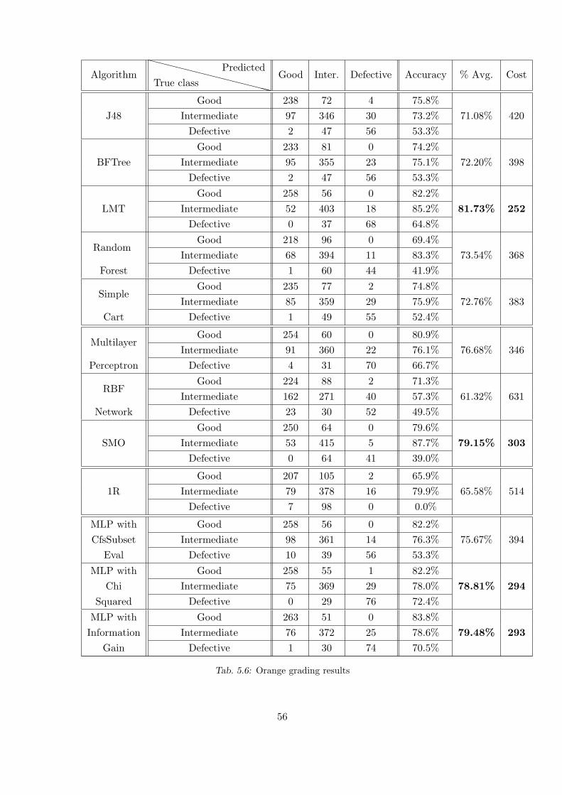
Algorithm
XX
XX
XX
XX
XX
XX
XX
True class
PredictedGood Inter. Defective Accuracy % Avg. Cost
J48
Good 238 72 4 75.8%
71.08% 420Intermediate 97 346 30 73.2%
Defective 2 47 56 53.3%
BFTree
Good 233 81 0 74.2%
72.20% 398Intermediate 95 355 23 75.1%
Defective 2 47 56 53.3%
LMT
Good 258 56 0 82.2%
81.73% 252Intermediate 52 403 18 85.2%
Defective 0 37 68 64.8%
RandomGood 218 96 0 69.4%
73.54% 368Intermediate 68 394 11 83.3%
Forest Defective 1 60 44 41.9%
SimpleGood 235 77 2 74.8%
72.76% 383Intermediate 85 359 29 75.9%
Cart Defective 1 49 55 52.4%
MultilayerGood 254 60 0 80.9%
76.68% 346Intermediate 91 360 22 76.1%
Perceptron Defective 4 31 70 66.7%
RBFGood 224 88 2 71.3%
61.32% 631Intermediate 162 271 40 57.3%
Network Defective 23 30 52 49.5%
SMO
Good 250 64 0 79.6%
79.15% 303Intermediate 53 415 5 87.7%
Defective 0 64 41 39.0%
1R
Good 207 105 2 65.9%
65.58% 514Intermediate 79 378 16 79.9%
Defective 7 98 0 0.0%
MLP with Good 258 56 0 82.2%
75.67% 394CfsSubset Intermediate 98 361 14 76.3%
Eval Defective 10 39 56 53.3%
MLP with Good 258 55 1 82.2%
78.81% 294Chi Intermediate 75 369 29 78.0%
Squared Defective 0 29 76 72.4%
MLP with Good 263 51 0 83.8%
79.48% 293Information Intermediate 76 372 25 78.6%
Gain Defective 1 30 74 70.5%
Tab. 5.6: Orange grading results
56

5.3 Conclusions
Once the segmentation process is finished, we apply several image processing techniques
to obtain several descriptors of that image, like area, fractal dimension, texture statistical
descriptors, color descriptors from histogram analysis, and statistical descriptors from the
HSV color space.
Then, in the classification step we apply nine data mining algorithms for orange quality
classification through visual features. The first group of algorithms are decision trees (J48,
Best First, Logistic Model Tree, Random Forest and Simple CART), the second group
consists of neural networks (Multilayer Perceptron, Radial Basis Function and Sequential
Minimal Optimization) and then a classification rule (1Rule) is analyzed.
The main advantage of decision trees and classification rules over neural networks are
their simplicity and interpretation of the obtained classification rules, as neural networks
work as a black box and the model produced by the algorithm are much more difficult to
interpret.
Although most of the algorithms produce good results (with an accuracy higher than
75%), the Logistic Model Tree, Sequential Minimal Optimization neural network and
Multilayer perceptron neural network with attribute selection are the ones which, in the
experiments done, produce the models with the highest accuracy (about 80%). Most of the
errors produced by the SMO algorithm are defective oranges misclassified as intermediate
ones (64 errors) and good oranges misclassified as intermediate ones (64 errors), while the
Logistic Model Tree misclassifies 56 good oranges as intermediate, 52 intermediate as good
and other misclassifications between intermediate and defective classes.
One of the drawbacks of SMO is that only 39% of the defective oranges are classified as
such, while with the LMT 64.6% of the defective oranges are correctly classified, and with
the Multilayer perceptron with attribute subset selection using Information Gain, 70.5%
of the oranges are correctly classified. However, MLP with Information Gain misclassifies
one defective orange as good.
Analyzing the results, we choose the Logistic Model Tree as the best classifier, because
not only it achieves the highest classification accuracy (81.73%) and the lowest cost (252),
but also the model produced by a Logistic Model Tree is easier to interpret by humans
compared to the one produced by the Multilayer perceptron and SMO neural networks.
On the opposite side, the algorithms with the worst accuracy are the Radial Basis
Function Network (61.32%), which misclassifies 23 defective oranges as good and 2 good
as defective, and the One Rule algorithm (65.58%), which misclassifies 2 good oranges as
defective and 7 defective as good.
57

6. CONCLUSIONS AND FUTURE WORKS
In the food industry, quality assurance processes can benefit from automated visual in-
spection, because it provides a uniform way of performing the classification, and free the
workers from the repetitive task of visually inspecting one by one all the harvested fruit.
Performing an accurate classification is crucial in order to fulfill the quality require-
ments established by several organizations to allow the commercialization of the fruits for
specific markets. If a good quality orange is misclassified as defective or intermediate, it
will be sold at a lower price, but if a defective orange is misclassified as good, it might
lead to the application of fines for selling defective oranges as good; or if the defect is an
illness, it can lead to discard the whole lot of fruits, causing a considerable loss of money.
The development of an automated orange grading system is not a trivial task, as the
defects found in the fruits can be of very different types and do not usually exhibit a known
pattern. Thus, they cannot be detected using conventional image processing techniques.
One of the most difficult tasks faced in fruit grading systems is the detection of the
calyx, which is necessary in order not to misclassify the calyx as a defect. A wrong
detection of the calyx would reduce the overall accuracy of the orange grading system,
either if it detects a calyx where in fact is a defect which will classify a defective orange
as good, or if it does not detect the calyx, downgrading the obtained category.
Along this thesis we have proven the feasibility of building an automatic orange grading
system using data mining and image processing techniques.
The process starts by capturing images from all possible angles using an inspection
chamber with a digital camera and a set of mirrors. Then, the background is removed
and a segmentation step which uses k-means clustering over the CIE L*a*b* color space
detects the candidate regions where it is likely to find a calyx. Next, Zernike Moments
and Principal Components features are extracted in order to build a dataset to be used
in the classification step to classify the region as a defect or a calyx. In this step, we
compare several machine learning algorithms, choosing the Logistic Model Tree as the
best classifier, because of its high accuracy across the different datasets and attributes
configuration, and also because of the easier interpretation of the model compared to the
neural networks.
Next, the quality categories classification subsystem receives as an input the image of
the orange with its calyx removed, where several geometric, textural and statistical fea-
tures are extracted, being the fractal dimension, the contrast attribute of the HSV color

space, the third range of the red component histogram and the fifth range of the green
component histogram some of the most relevant features obtained. With these features, in
the classification step we build a dataset and apply several machine learning algorithms,
being the Logistic Model Tree, Sequential Minimal Optimization neural network and Mul-
tilayer Perceptron neural network with Backpropagation the classifiers which achieve the
best classification rates.
Most of this work can also be applied to classifying other kinds of fruit, specially citrus.
However, several adjustments should be done depending on the color, shape, texture and
other features of the fruit. Also, the data mining algorithms should be retrained in order
to learn the new kind of problem. We intend to analyze the application of the system to
other types of fruits in a future research.
Another area we are interested in is to classify the detected defects into different
categories of defects and identify illnesses.
In a future work, we will optimize the processing speed of the algorithms. To do this, it
will be necessary to measure the amount of oranges classified in a certain amount of time,
like for example the amount of oranges classified per second. This will be done taking into
account the speed requirements of real production lines.
We are also interested in implementing in the future the image capture subsystem and
classified oranges placement subsystem in order to integrate all the hardware and software
components and be able to test the whole orange grading system in real production lines.
59

BIBLIOGRAPHY
[1] Gholamreza A., Ali E., George B., and Mircea N. Accurate and efficient computation
of high order Zernike moments. In ISVC, pages 462–469, 2005.
[2] Khotanzad A. and Hong Y. H. Invariant image recognition by Zernike moments.
IEEE Trans. Pattern Anal. Mach. Intell., 12(5):489–497, 1990.
[3] Palak K. A. and Koduvayur P. S. Rotation and cropping resilient data hiding with
Zernike moments. In ICIP, pages 2175–2178, 2004.
[4] Wiliem A., Vamsi K., Wageeh B., and Prasad Y. A face recognition approach using
Zernike moments for video surveillance. In RNSA Security Technology Conference,
Melbourne, Australia, 2007.
[5] Wiliem A., Vamsi M., Wageeh B., and Prasad Y. Eye detection in facial images
using Zernike moments with SVM. In RNSA Security Technology Converence 2007,
School of Engineering Systems, Queensland University of Technology, pages 341–355,
Melbourne, Australia, 2007.
[6] Galiano F. B. ART: Un metodo alternativo para la construccion de arboles de decision.
PhD thesis, Departamento de Ciencias de la Computacion e Inteligencia Artificial,
Ingenierıa Informatica, Universidad de Granada, 2002.
[7] Caiafa C. and Proto A. N. Desarrollo de un software para la identificacion de elefantes
marinos por eigenfaces. In Reportes Tecnicos en Ingenierıa del Software, volume 5,
pages 27–40. CAPIS-EPG-ITBA, 2003.
[8] Jensen D. and Cohen P. Multiple comparisons in induction algorithms. Machine
Learning, pages 309–338, 1997.
[9] Mery D. Inspeccion visual automatica. In Actas del 1er Congreso Internacional de
Ingenierıa Mecatronica, Lima, Peru, 2002.
[10] Unay D. and Gosselin B. Apple defect detection and quality classification with MLP-
Neural Networks. In International workshop ProRISC 2002 (Circuits, Systems and
Signal Processing), 2002.
[11] Unay D. and Gosselin B. Stem-end/calyx detection in apple fruits: Comparison of
feature selection methods and classifiers. In Proc. Int. Conf. Computer Vision and
Graphics (ICCVG), 2004.
[12] Johnson D. E. Metodos multivariados aplicados al analisis de datos. International
Thomson Editores, 1998.
[13] Canny F. A computational approach to edge detection. IEEE-PAMI, 8(6):679–698,
1986.
[14] Lopez F., Valiente J. M., and Caselles R. B.and Vanrell M. Fast surface grading
using color statistics in the CIE Lab space. Lecture Notes in Computer Science,
3523:666–673, 2005.
[15] Provost F., Fawcett T., and Kohavi R. The case against accuracy estimation for
comparing induction algorithms. In In Proceedings of the Fifteenth International
Conference on Machine Learning, pages 445–453. Morgan Kaufmann, 1997.
[16] Jan H. and Kamber M. Data Mining: Concepts and Techniques. Morgan Kaufmann,
2000.
[17] Zubrzycki H. and Molina. Factibilidad comercial de cıtricos entre Argentina y Brasil.
In Publicacion de la EEA Bella Vista Serie Tecnica No 17, 2005.
[18] Witten I. and Frank E. Data Mining: Practical Machine Learning Tools and Tech-
niques. Second Edition. Morgan Kaufmann, 2005.
[19] Hertz J., Krogh A., and Palmer R. Introduction to the Theory of Neural Computation.
Wesley Publishing Co., 1991.
[20] Xing J., Jancsok P., and Baerdemaeker J. Stem-end/calyx identification on apples
using contour analysis in multispectral images. Biosystems engineering, pages 231–
237, 2007.
[21] B. Jahne. Digital Image Processing: Concepts, Algorithms, and Scientific Applica-
tions. Springer-Verlag New York, Inc., Secaucus, NJ, USA, 1997.
[22] D. N. Joanes and C. A. Gill. Comparing measures of sample skewness and kurtosis.
Journal of the Royal Statistical Society: Series D (The Statistician), 47(1):183–189,
1998.
[23] Mercol J.P. and Gambini M. J. Stem-end/calyx detection in oranges using image
processing and data mining techniques. XIII Reunion de trabajo en Procesamiento
de la Informacion y Control (RPIC), pages 141–146, September 2009.
[24] Mercol J.P., Gambini M. J., and Santos J. M. Clasificacion automatica de naranjas
por medio de imagenes utilizando tecnicas de data mining. Jornadas Chilenas de
Computacion 2008, 2008.
[25] Mercol J.P., Gambini M. J., and Santos J. M. Automatic classification of oranges
using image processing and data mining techniques. XIV Congreso Argentino de
Ciencias de la Computacion, October 2008.
61

[26] Erum A. K. and Erik R. A survey of color spaces for shadow identification. In
APGV ’04: Proceedings of the 1st Symposium on Applied perception in graphics and
visualization, pages 160–160, New York, NY, USA, 2004. ACM.
[27] Falconer K. Fractal Geometry: Mathematical Foundations and Applications. John
Wiley & Sons, Chichester, England, 1990.
[28] Forbes K. Volume estimation of fruits from digital profile images. PhD thesis, De-
partment of Electrical Engineering, University of Cape Town, Cape Town, 2000.
[29] Hyoung-Joon K. and Whoi-Yul K. Eye detection in facial images using Zernike mo-
ments with SVM. ETRI Journal, 30(2):335–337, Apr. 2008.
[30] Breiman L. Random forests. Machine Learning, 45(1):5–32, 2001.
[31] Breiman L., Friedman J.H., Olshen R.A., and Stone C J. Classification and Regression
Trees. Wadsworth Publishing Company, Belmont, California, USA, 1984.
[32] Jin C. L., Ling C. X., Huang J., and Zhang H. AUC: a statistically consistent and
more discriminating measure than accuracy. In In Proceedings of 18th International
Conference on Artificial Intelligence (IJCAI-2003), pages 329–341, 2003.
[33] Lopez-Conejo L. and Sanchez-Yanez R. Segmentacion de imagenes naturales usando
el espacio de color CIE Lab. III Encuentro Participacion de la Mujer en la Ciencia,
May 2006.
[34] Ruiz L.A., Molto E., Juste F., Pla F., and Valiente R. Location and characteriza-
tion of the stem-calyx area on oranges by computer vision. Journal of Agricultural
Engineering Research, 64:165–172(8), July 1996.
[35] Fernandez Ribot M. Selector de fruta y simulacion de una aplicacion real. PhD thesis,
Universidad Politecnica de Catalunya, Espana, 2006.
[36] Mitchell T. M. Machine Learning. McGraw-Hill, 1997.
[37] Recce M., Taylor J., Plebe A., and Tropiano G. High speed vision-based quality grad-
ing of oranges. In NICROSP ’96: Proceedings of the 1996 International Workshop
on Neural Networks for Identification, Control, Robotics, and Signal/Image Process-
ing (NICROSP ’96), pages 136–144, Washington, DC, USA, 1996. IEEE Computer
Society.
[38] Servente M. and Garcıa Martinez R. Algoritmos TDIDT aplicados a la mineria de
datos inteligentes. Revista Del Instituto Tecnologico de Buenos Aires, 26:39–57, 2002.
[39] Twa M., Parthasarathy S., Rosche T., and Bullmer M. Decision tree classification
of spatial data patterns from videokeratography using Zernike polynomials. SIAM
International Conference on Data Mining, 2003.
62
[40] Hall M.A. and L. A. Smith. Feature subset selection: A correlation based filter
approach. In Conf. on Neural Information Processing and Intelligent Information
Systems, pages 855–858, Hamilton, New Zealand, 1997. Springer (Ed.).
[41] Donald Michie, D. J. Spiegelhalter, C. C. Taylor, and John Campbell, editors. Ma-
chine learning, neural and statistical classification. Ellis Horwood, Upper Saddle
River, NJ, USA, 1994.
[42] Landwehr N., Hall M., and Frank E. Logistic model trees. In Machine Learning,
pages 241–252. Springer-Verlag, 2003.
[43] Marques N. and Chen N. Border detection on remote sensing satellite data using
Self-Organizing Maps. In Pires F.M., Abreu S.(Eds.): EPIA 2003, LNAI 2902.
Spinger-Verlag Berlin Heidelberg., pages 294–307, 2003.
[44] N. Nilsson. Introduction to Machine Learning. MIT Press (to appear), 1998.
[45] D’Amato J. P., Garcıa B. C., Venere M., and Clausse A. Procesamiento de imagenes
para la clasificacion masiva de frutos basado en el color. In Universidad Nacional del
Centro, CNEA-CICPBA-CONICET, 2007.
[46] Gay P., Berruto R., and Piccarolo P. Fruit color assessment for quality grading
purposes. In ASAE Annual International Meeting/ CIGR XVth World Congress,
pages 28–31, Chicago, Illinois, USA, 2002.
[47] J. C. Platt. Fast training of support vector machines using sequential minimal opti-
mization. MIT Press, Cambridge, MA, USA, 1999.
[48] Kohavi R. A study of cross-validation and bootstrap for accuracy estimation and
model selection. In IJCAI, pages 1137–1145, 1995.
[49] Gonzalez R.C., Woods R., and Eddins S. Digital Image Processing Using MATLAB.
Pearson Prentice-Hall, 2004.
[50] Holte R.C. Very simple classification rules perform well on most commonly used
datasets. Mach. Learn., 11(1):63–90, 1993.
[51] Haijian S. Best-first decision tree learning. Master’s thesis, University of Waikato,
Hamilton, NZ, 2007. COMP594.
[52] Haykin S. Neural Networks. A Comprehensive Foundation Second Edition. Prentice
Hall International Inc, 1999.
[53] Carg A. Sebe N., Cohen I. and Huang T. Machine Learning in Computer Vision.
Springer, 2005.
[54] Chen S.S., Keller J.M., and Crownover R.M. On the calculation of fractal features
from images. Pattern Analysis and Machine Intelligence, 15(10):1087–1090, 1993.
63

[55] Fawcett T. ROC graphs: Notes and practical considerations for researchers. Kluwer
Academic Publishers, 2004.
[56] Morimoto T., Takeuchi T., Miyata H., and Hashimoto Y. Pattern recognition of fruit
shape based on the concept of chaos and neural networks. Computers and Electronics
in Agriculture, pages 171–186, 2000.
[57] Liu Y. and Li Y. Image feature extraction and segmentation using fractal dimension.
In International Conference on Information and Signal Processing, pages 975–979,
Singapur, 1997. IEEE.
64