universidad complutense de madrid - core · bel en (carla) por aguantarme cuando entro en panico,...
TRANSCRIPT
UNIVERSIDAD COMPLUTENSE DE MADRID
FACULTAD DE INFORMATICA Departamento de Sistemas Informáticos y Computación
TESIS DOCTORAL
Sobre la equivalencia entre semánticas operacionales y denotacionales
para lenguajes funcionales paralelos
MEMORIA PARA OPTAR AL GRADO DE DOCTOR
PRESENTADA POR
Lidia Sánchez Gil
Directores
Mercedes Hidalgo Herrero Yolanda Ortega Mallén
Madrid, 2015
© Lidia Sánchez Gil, 2015
Sobre la equivalencia entre semanticasoperacionales y denotacionales para
lenguajes funcionales paralelos
TESIS DOCTORAL
Memoria presentada para optar al grado de Doctor
Presentada por
Lidia Sanchez Gil
Dirigida por las doctoras
Mercedes Hidalgo Herrero
Yolanda Ortega Mallen
Departamento de Sistemas Informaticos y Computacion
Facultad de Informatica
Universidad Complutense de Madrid
2015

On the equivalence of operational anddenotational semantics for parallel
functional languages
PhD Thesis
Lidia Sanchez Gil
Advisors
Mercedes Hidalgo Herrero
Yolanda Ortega Mallen
Departamento de Sistemas Informaticos y Computacion
Facultad de Informatica
Universidad Complutense de Madrid
2015

Agradecimientos
Tengo tanto que agradecer y a tantas personas que podrıa rellenar paginas y paginas yaun me faltarıa espacio. A lo largo de estos anos han sido muchos los que me han ayudadoy es imposible nombrar a todos. Ası que he tenido que hacer una criba y quedarme conlos mas significativos.
En primer lugar quiero dar las gracias a Carlos, por estar ahı dıa a dıa, por aguantarme,por ocuparse de la casa y el peque para que yo pueda terminar con lo que ya empece. Leconocı antes de empezar este proyecto y durante este tiempo ha vivido los altibajos deeste largo camino. Con el he compartido los buenos momentos y el me ha hecho ver la otracara de la moneda en los no tan buenos, pero siempre respetando mis decisiones. Me haescuchado mil y una vez mientras yo pensaba en alto para ver si ası conseguıa aclarar misideas. Ha llevado con una sonrisa que no le contestara por estar pensando en mis cosas.Gracias por ser un marido fabuloso sin el cual yo no estarıa aquı. Y gracias a Ezequiel que,sin saberlo, ha puesto su granito de arena prescindiendo de mami muchos dıas y muchasnoches.
Tambien tengo que dar las gracias a esas maravillosas personas que me trajeron almundo, mis papis, Luis y Rosa. Les agradezco todo lo que han hecho y siguen haciendopor mı. Por sus esfuerzos, a veces grandes, a veces pequenos, para darnos una educaciony ensenarnos la suerte que tenemos de poder disfrutar de ella. Por su apoyo economico yel no economico que es, sin duda alguna, mucho mayor que el primero.
Y como esto va de familia, pues no puedo dejarme a mis hermanas. A Lucıa por tenerlacerquita, a ella, a Juan Carlos y a Carlos y Rosa, por hacerme pasar buenos ratos cuandoestamos juntos y suavizar los momentos de tension disfrutando de buena companıa. AIgnicia por la lejanıa, por mostrarme que el estar lejos no es sinonimo de olvido o de noquerer. A ella y a todas las hermanas de Belen que he conocido en estos anos les doy lasgracias por su interes y por sus oraciones.
Tambien agradezco a mi familia polıtica su ayuda. En especial a mis suegros, Concha yGonzalo, por venir a cuidar a Ezequiel mientras Carlos y yo curramos, y a Coty, la pequede la family por esas charlas interminables, por compartir conmigo un monton de risas ypor hacer reır a Ezequiel como nadie.
Y aunque los agradecimientos a la familia podrıan extenderse tanto como extensa esen sı misma, pasare al grupo de amigos. Primero agradecerle a Monica su amistad desde lainfancia. Crecimos juntas y nos fuimos formando a la par, con nuestras vidas paralelas, tandistintas y tan iguales a la vez. Tenıamos claro desde el principio lo que querıamos y por loque luchar y bueno, quiza no todos, pero parte de esos suenos se han ido cumpliendo. Pesea que lo que llamamos la vida de adulto no nos permite vernos tanto como quisieramossiempre, siempre, ha estado a golpe de telefono y dispuesta a escucharme y quedar parainvitarme a zumito de naranja. Y el pack Monica-Lidia, se queda cojo sin el gran Ignacio
v
vi
(Nacho para todos menos para nosotras). Hemos sido como hermanos, incluso llegamosa inventarnos nuestros propios apellidos para pasar como tales en los campamentos dela infancia, y a dıa de hoy sigue ahı, alegrandose de mis logros pese a querer usurparlela Senora Cucharita. Y a ambos os agradezco gran parte de lo que soy, pese a llamarme“bruja”.
A mis queridas Penita (y Juan) y Gemita, tambien tengo que agradecerles que hayallegado hasta aquı. Muchas horas de estudio compartidas y mucho apoyo y animos durantetodo este tiempo. A mis dos grupos de mamas, en particular a Isa, Leti, Gema, Cami yBelen (Carla) por aguantarme cuando entro en panico, por prestarme vuestro apoyo y porayudarme a buscar sinonimos que encajen en el texto. A todo ese gran monton de amigosque han rezado por mı y que no voy a nombrar por ser una lista demasiado grande.
Y pasamos a las personas de ciencia. Aliseta, que podrıa encajar perfectamente enel grupo de amigos de antano pero ha terminado estando en este lado. Gracias por esosenormes desayunos con zumo de naranja, cafe y barrita de jamon serrano a la plancha conqueso fundido, complementados en ocasiones con un donuts de azucar y otro de chocolate,que me sacaban de los bloqueos mentales y alimentaban mi cuerpo y mi espıritu. Gra-cias por tus consejos y por calmarme en los momentos de estres. Otro de los personajesimportantes de esta historia ha sido el gran, fabuloso y magnıfico Ignacio Fabregas (nome odies por esto). Le conocıa desde hacıa bastante pero Marktdoberdorf me descubrio lagran persona que es y todo lo que sabe. Es mi pequeno dios, sacandome de apuros cadados por tres, esta siempre dispuesto a ayudar, y no solo eso, es que ayuda de verdad. Meha ayudado con la ciencia, con el dichoso LaTeX, y con un monton de charlas ameniza-doras. Con David Chico he tratado menos que con Ignacio pero ha sido un companero dedespacho fabuloso y sı, tambien saca de apuros. David de Frutos es como un padre de laciencia, si tienes una duda sabes que puedes recurrir a el, sabe de todo y siempre tiene undato importante, un artıculo interesante o unos comentarios que ayudan a perfeccionar lohecho. Aunque en menor medida tambien han dejado su marca personas como Luis Llana,Maria Ines, Jorge Carmona, Alberto E. y Alberto V., mis companeros de Master ManuelMontenegro y Carlos Romero y otros companeros de escuelas y congresos como Gaby,Nacho, Enrique, Adrian (que tambien me ha prestado gran ayuda en temas de papeleo),Henrique y Castro. Tambien quiero agradecer los comentarios y consejos de Rita Loogen,Phil Trinder, Joachim Breitner y Arthur Chargueraud.
Yolanda y Mercedes, dos grandes mujeres y dos grandes directoras. Mucho ha sidoel tiempo que me han dedicado. A veces, lo han tenido que sacar del tiempo dedicado asus familias, por lo que este agradecimiento se hace extensible a Luis, Fernando, Jorge,Daniel y la pequena Ana. Les doy las gracias por haber creıdo en este sueno incluso masque yo misma, por todo lo que me han ensenado tanto en lo referente a ciencia comoen lo referente a la vida, por haberme guiado durante todo este largo camino, por haberconseguido de mı lo que no hubiera hecho jamas por mı misma.
Y aquı va el ultimo agradecimiento, aunque me atreverıa a decir que el mas importantede todos. Todas las personas mencionadas anteriormente (y muchas de las no mencionadas)han contribuido a que yo este aquı. Pero como casi todo doctorando hay momentos en losque uno quiere tirar la toalla y dedicarse a otros menesteres, y no soy menos que los demas,pero en mi caso podrıa decir que llegue a tirar la toalla. Muchos trataron de convencerme yde que siguiera adelante, pero mi decision estaba tomada. Entre en el despacho de NarcisoMartı Oliet a decirle que todo se terminaba y, aun no se como, salı con la determinacionde que terminarıa la tesis. No ha pasado ni un solo dıa en el que no le haya agradecido suspalabras, que seguiran en mi interior como han estado todo este tiempo. Solamente puedodecir GRACIAS.

vii
Para concluir he de decir que mi tesis ha formado parte de los proyectos de inves-tigacion: StrongSoft (TIN2012-39391-C04-04) financiado por el Ministerio de Economıay Competitividad, PROMETIDOS (S2009/TIC-1465) financiado por la Comunidad deMadrid, DESAFIOS10 (TIN2009-14599-C03-01) financiado por el Ministerio de Ciencia eInnovacion, DESAFIOS (TIN2006-15660-C02-01) financiado por el Ministerio de Educa-cion y Ciencia, WEST(TIN2006-15578-C02-01) financiado por el Ministerio de Educaciony Ciencia, PROMESAS (ref. S-0505/TIC-0407) financiado por la Comunidad de Madridy la ayuda predoctoral FPI (BES-2007-16823) financiada por el Ministerio de Educaciony Ciencia.

viii
Resumen
Tal y como se indica en [ede14], Eden es un lenguaje funcional paralelo que extiendeHaskell con construcciones sintacticas para especificar la creacion de procesos. Como ex-plican los autores de [BLOP96], en Eden se distinguen dos partes: un λ-calculo perezoso yexpresiones de coordinacion. El lenguaje Jauja es una simplificacion de Eden que mantie-ne sus principales caracterısticas. El objetivo de esta tesis es dar los primeros pasos parademostrar la equivalencia entre las semanticas definidas para Jauja por Hidalgo-Herreroen [Hid04]. Se quiere probar la equivalencia en terminos de correccion y adecuacion compu-tacional entre una semantica operacional y una semantica denotacional. Para hacerlo nosbasamos en las ideas expuestas por Launchbury en [Lau93], en el que se demuestra laequivalencia entre una semantica natural y una semantica denotacional estandar para unλ-calculo extendido con declaraciones locales.
Puesto que demostrar la equivalencia entre las semanticas definidas para Jauja suponeun estudio demasiado complejo para afrontarlo en un primer paso, hemos comenzado porconsiderar una extension del lenguaje utilizado por Launchbury al que se ha anadido unaaplicacion paralela que da lugar a creaciones de procesos y comunicaciones entre ellos, esdecir, a un sistema distribuido formado por distintos procesos que interactuan entre sı.A partir de este sencillo lenguaje el estudio se desarrolla en varias etapas en las que seestablece la equivalencia entre distintas semanticas operacionales y denotacionales paramodelos distribuidos y no distribuidos. La semantica operacional del modelo distribuidoheredada de Jauja es una semantica de paso corto para varios procesadores. Para reali-zar la equivalencia de esta semantica con una semantica denotacional estandar extendida,con objeto de dotar de significado a la aplicacion paralela, se introducen dos semanticasintermedias: una de paso corto pero limitada a un unico procesador y una semantica depaso largo que es una extension de la semantica natural de Launchbury. En el caso deprescindir de las aplicaciones paralelas, la semantica natural de Launchbury y nuestraextension se comportan igual. Con respecto al modelo no distribuido, y con el fin de com-pletar las demostraciones ausentes en el trabajo de Launchbury, se construye un espaciode funciones para los valores de la semantica denotacional con recursos introducida porel autor. Posteriormente, se comprueba que es equivalente a la semantica denotacionalestandar bajo la condicion de disponer de infinitos recursos. Tambien se estudian algunasrelaciones existentes entre heaps y pares (heap, termino) que se aplican para estudiar laequivalencia de las dos semanticas operacionales introducidas por Launchbury.
Hemos realizado gran parte del estudio utilizando la notacion localmente sin nombres,situada a medio camino entre la de nombres y la de de Bruijn. Ası se evitan los pro-blemas derivados de la notacion con nombres, es decir, tener que trabajar con terminosα-equivalentes. Por otra parte, tambien se eluden las desventajas de utilizar solo los ındicesde de Bruijn, que resultan complicados de manejar y dificultan la lectura de los terminos.
ix

x
Abstract
The programming language Eden [ede14] is a parallel functional language that extendsHaskell with some syntactic constructs for explicit process specification and creation.Eden [BLOP96] comprises two differentiated parts: A lazy λ-calculus and coordinationexpressions. The programming language Jauja is a simplification of Eden that gathers itsmain characteristics. The target of this thesis is to give the first steps in the proof of theequivalence between the semantics defined for Jauja by Hidalgo-Herrero in [Hid04]. Weprove the equivalence in terms of correctness and computational adequacy of an operationalsemantics with respect to a denotational one. We base our work on Launchbury’s ideas thatare introduced in [Lau93], where he proved the equivalence between a natural semanticsand a standard denotational semantics for a λ-calculus extended with local declarations.
Since the study of the equivalence between the semantics defined for Jauja is toocomplex, we start with the study of the language used by Launchbury extended with aparallel application. This new expression gives rise to the creation of processes and thecommunication between them, i.e., to a distributed model with several processes. Thestudy is developed in several steps, with different operational and denotational semanticsfor distributed and non-distributed models.
The operational semantics of the distributed model inherited from Jauja is a small-stepsemantics for several processors. In order to prove the equivalence between this semanticsand an extension of the standard denotational semantics, we introduce two intermedi-ate semantics: A small-step semantic restricted to one processor, and an extension ofLaunchbury’s natural semantics. When no parallel application is involved, Launchbury’sextension and the original natural semantics have the same behavior.
The study of the non-distributed model leads to the construction of an appropri-ate function space for the values of the resourced denotational semantics introduced byLaunchbury. This resourced semantics and the standard denotational one are equivalentwhen infinitely many resources are provided. We also define a preorder relation on heaps,that is extended to (heap, term) pairs. We use this preorder to establish a relation be-tween the heaps and values produced when the same (heap, term) pair is evaluated withdifferent semantics.
We use the locally nameless representation, which is halfway between the named no-tation and the de Bruijn notation. This alternative avoids the problems derived fromthe named representation, i.e., dealing with α-equivalence, as well as the disadvantages ofusing only indices.
xi


Indice general
I Resumen de la Investigacion 1
1 ¿Que, por que y como? 3
1.1 Objetivos de la tesis . . . . . . . . . . . . . . . . . . . . . . . . . . . . . . . 4
1.2 Organizacion de la tesis . . . . . . . . . . . . . . . . . . . . . . . . . . . . . 4
2 ¿Que estaba hecho? 7
2.1 Lenguajes de programacion . . . . . . . . . . . . . . . . . . . . . . . . . . . 7
2.1.1 Lenguajes de programacion funcionales . . . . . . . . . . . . . . . . 7
2.1.2 Estrategias de evaluacion . . . . . . . . . . . . . . . . . . . . . . . . 8
2.1.3 Lenguajes funcionales paralelos . . . . . . . . . . . . . . . . . . . . . 9
2.1.4 El lenguaje funcional paralelo Eden . . . . . . . . . . . . . . . . . . . 9
2.2 Semanticas de lenguajes de programacion . . . . . . . . . . . . . . . . . . . 10
2.2.1 Semanticas formales . . . . . . . . . . . . . . . . . . . . . . . . . . . 10
2.3 Espacios de funciones . . . . . . . . . . . . . . . . . . . . . . . . . . . . . . 11
2.3.1 Conceptos basicos . . . . . . . . . . . . . . . . . . . . . . . . . . . . 11
2.3.2 Construccion de la solucion inicial . . . . . . . . . . . . . . . . . . . 12
2.3.3 Bisimulacion Aplicativa . . . . . . . . . . . . . . . . . . . . . . . . . 14
2.4 Semantica natural para evaluacion perezosa . . . . . . . . . . . . . . . . . . 14
2.4.1 Propiedades . . . . . . . . . . . . . . . . . . . . . . . . . . . . . . . . 17
2.5 El lenguaje Jauja y las semanticas formales de Eden . . . . . . . . . . . . . 18
2.5.1 Semantica Operacional . . . . . . . . . . . . . . . . . . . . . . . . . . 18
2.5.2 Semantica Denotacional . . . . . . . . . . . . . . . . . . . . . . . . . 19
2.6 Representaciones del λ-calculo . . . . . . . . . . . . . . . . . . . . . . . . . . 20
2.6.1 Notacion de de Bruijn . . . . . . . . . . . . . . . . . . . . . . . . . . 20
2.6.2 Representacion localmente sin nombres . . . . . . . . . . . . . . . . 21
2.7 Asistentes de demostracion . . . . . . . . . . . . . . . . . . . . . . . . . . . 23
3 ¿Que hemos obtenido? 25
3.1 Adecuacion computacional . . . . . . . . . . . . . . . . . . . . . . . . . . . . 25
3.1.1 Espacio de funciones con recursos . . . . . . . . . . . . . . . . . . . . 26
3.1.2 Semantica natural alternativa . . . . . . . . . . . . . . . . . . . . . . 29
3.2 Modelo Distribuido . . . . . . . . . . . . . . . . . . . . . . . . . . . . . . . . 37
3.3 Trabajos relacionados . . . . . . . . . . . . . . . . . . . . . . . . . . . . . . 42
3.4 Conclusiones . . . . . . . . . . . . . . . . . . . . . . . . . . . . . . . . . . . 44
xiii
4 ¿Que queda por hacer? 47
4.1 Equivalencia NS y NNS . . . . . . . . . . . . . . . . . . . . . . . . . . . . . 48
4.2 Equivalencias entre NS y INS y entre INS y ANS . . . . . . . . . . . . . . . 50
4.3 Extension al modelo distribuido . . . . . . . . . . . . . . . . . . . . . . . . . 51
4.4 Implementacion en Coq . . . . . . . . . . . . . . . . . . . . . . . . . . . . . 51
II Summary of the Research 55
1 What, why and how? 57
1.1 Objectives . . . . . . . . . . . . . . . . . . . . . . . . . . . . . . . . . . . . . 58
1.2 Summary . . . . . . . . . . . . . . . . . . . . . . . . . . . . . . . . . . . . . 58
2 What was done? 61
2.1 Programming languages . . . . . . . . . . . . . . . . . . . . . . . . . . . . . 61
2.1.1 Functional Programming Languages . . . . . . . . . . . . . . . . . . 61
2.1.2 Evaluation strategies . . . . . . . . . . . . . . . . . . . . . . . . . . . 62
2.1.3 Parallel functional languages . . . . . . . . . . . . . . . . . . . . . . 62
2.1.4 The functional parallel language Eden . . . . . . . . . . . . . . . . . 63
2.2 Programming Language Semantics . . . . . . . . . . . . . . . . . . . . . . . 64
2.2.1 Formal semantics . . . . . . . . . . . . . . . . . . . . . . . . . . . . . 64
2.3 Function spaces . . . . . . . . . . . . . . . . . . . . . . . . . . . . . . . . . . 64
2.3.1 Basic concepts . . . . . . . . . . . . . . . . . . . . . . . . . . . . . . 65
2.3.2 Construction of the initial solution . . . . . . . . . . . . . . . . . . . 65
2.3.3 Applicative bisimulation . . . . . . . . . . . . . . . . . . . . . . . . . 67
2.4 Natural semantics for lazy evaluation . . . . . . . . . . . . . . . . . . . . . . 68
2.4.1 Properties . . . . . . . . . . . . . . . . . . . . . . . . . . . . . . . . . 70
2.5 The language Jauja and the formal semantics of Eden . . . . . . . . . . . . 71
2.5.1 Operational Semantics . . . . . . . . . . . . . . . . . . . . . . . . . . 71
2.5.2 Denotational semantics . . . . . . . . . . . . . . . . . . . . . . . . . 72
2.6 λ-calculus representations . . . . . . . . . . . . . . . . . . . . . . . . . . . . 73
2.6.1 The de Bruijn notation . . . . . . . . . . . . . . . . . . . . . . . . . 73
2.6.2 Locally nameless representation . . . . . . . . . . . . . . . . . . . . . 74
2.7 Proof assistants . . . . . . . . . . . . . . . . . . . . . . . . . . . . . . . . . . 75
3 What have we got? 77
3.1 Computational adequacy . . . . . . . . . . . . . . . . . . . . . . . . . . . . . 77
3.1.1 Function space with resources . . . . . . . . . . . . . . . . . . . . . . 78
3.1.2 Alternative natural semantics . . . . . . . . . . . . . . . . . . . . . . 81
3.2 Distributed Model . . . . . . . . . . . . . . . . . . . . . . . . . . . . . . . . 88
3.3 Related work . . . . . . . . . . . . . . . . . . . . . . . . . . . . . . . . . . . 92
3.4 Conclusions . . . . . . . . . . . . . . . . . . . . . . . . . . . . . . . . . . . . 94
4 What is left to be done? 97
4.1 Equivalence of NS and NNS . . . . . . . . . . . . . . . . . . . . . . . . . . . 97
4.2 Equivalence of NS and INS, and of INS and ANS . . . . . . . . . . . . . . . 100
4.3 Extension to a distributed model . . . . . . . . . . . . . . . . . . . . . . . . 100
4.4 Implementation in Coq . . . . . . . . . . . . . . . . . . . . . . . . . . . . . 101
III Publicaciones 107
5 Publicaciones 109P1 Relating function spaces to resourced function spaces . . . . . . . . . . . . . . 111P2 A locally nameless representation for a natural semantics for lazy evaluation . 119P3 The role of indirections in lazy natural semantics . . . . . . . . . . . . . . . . 135P4 An operational semantics for distributed lazy evaluation . . . . . . . . . . . . 151
Apendice 167
A Versiones extendidas 167TR1 A locally nameless representation for a natural semantics for lazy evaluation 169TR2 The role of indirections in lazy natural semantics . . . . . . . . . . . . . . . 199
B Trabajo en progreso 249WP1 Launchbury’s semantics revisited: On the equivalence of context-heap se-
mantics . . . . . . . . . . . . . . . . . . . . . . . . . . . . . . . . . . . . . . 251WP2 A formalization in Coq of Launchbury’s natural semantics for lazy evaluation267

Indice de figuras
2.1 Primeros niveles del espacio de funciones [D → D]⊥ . . . . . . . . . . . . . 132.2 Inyecciones y proyecciones entre niveles . . . . . . . . . . . . . . . . . . . . 132.3 Relacion binaria en Λ0 . . . . . . . . . . . . . . . . . . . . . . . . . . . . . . 142.4 Sintaxis restringida del λ-calculo extendido . . . . . . . . . . . . . . . . . . 152.5 Normalizacion del λ-calculo extendido . . . . . . . . . . . . . . . . . . . . . 152.6 Semantica natural . . . . . . . . . . . . . . . . . . . . . . . . . . . . . . . . 162.7 Semantica denotacional . . . . . . . . . . . . . . . . . . . . . . . . . . . . . 162.8 Semantica natural alternativa . . . . . . . . . . . . . . . . . . . . . . . . . . 172.9 Semantica denotacional con recursos. . . . . . . . . . . . . . . . . . . . . . . 172.10 Sintaxis de Jauja . . . . . . . . . . . . . . . . . . . . . . . . . . . . . . . . . 182.11 Modelo distribuido . . . . . . . . . . . . . . . . . . . . . . . . . . . . . . . . 192.12 Ejemplo de de Bruijn . . . . . . . . . . . . . . . . . . . . . . . . . . . . . . . 212.13 λ-calculo, representacion localmente sin nombres . . . . . . . . . . . . . . . 22
3.1 Idea de similaridad . . . . . . . . . . . . . . . . . . . . . . . . . . . . . . . . 283.2 Sintaxis localmente sin nombres . . . . . . . . . . . . . . . . . . . . . . . . . 303.3 Declaracion local de variables (notacion localmente sin nombres) . . . . . . 323.4 Sintaxis . . . . . . . . . . . . . . . . . . . . . . . . . . . . . . . . . . . . . . 383.5 Conversion de un modelo distribuido a uno que no lo es . . . . . . . . . . . 393.6 Conversion de un modelo no distribuido a uno que sı lo es . . . . . . . . . . 403.7 Esquema de conversion de heaps . . . . . . . . . . . . . . . . . . . . . . . . 41
2.1 First three levels of the function space [D → D]⊥ . . . . . . . . . . . . . . . 662.2 Injections and projections between levels . . . . . . . . . . . . . . . . . . . . 672.3 Binary relation in Λ0 . . . . . . . . . . . . . . . . . . . . . . . . . . . . . . . 672.4 Restricted syntax of the extended λ-calculus . . . . . . . . . . . . . . . . . . 682.5 Normalization of the extended λ-calculus . . . . . . . . . . . . . . . . . . . 682.6 Natural semantics . . . . . . . . . . . . . . . . . . . . . . . . . . . . . . . . 692.7 Denotational Semantics . . . . . . . . . . . . . . . . . . . . . . . . . . . . . 692.8 Alternative natural semantics . . . . . . . . . . . . . . . . . . . . . . . . . . 702.9 Resourced denotational semantics. . . . . . . . . . . . . . . . . . . . . . . . 702.10 Jauja syntax . . . . . . . . . . . . . . . . . . . . . . . . . . . . . . . . . . . 712.11 Distributed model . . . . . . . . . . . . . . . . . . . . . . . . . . . . . . . . 722.12 A de Bruijn example . . . . . . . . . . . . . . . . . . . . . . . . . . . . . . . 742.13 λ-calculus, locally nameless representation . . . . . . . . . . . . . . . . . . . 74
3.1 Intuition of similarity . . . . . . . . . . . . . . . . . . . . . . . . . . . . . . 80
xvii

xviii
3.2 Locally nameless syntax . . . . . . . . . . . . . . . . . . . . . . . . . . . . . 823.3 Variable local declaration (locally nameless representation) . . . . . . . . . 833.4 Syntax . . . . . . . . . . . . . . . . . . . . . . . . . . . . . . . . . . . . . . . 883.5 Coversion of a distributed system into a heap . . . . . . . . . . . . . . . . . 903.6 Coversion of a non-distributed model into a distributed one . . . . . . . . . 903.7 Conversion of heaps . . . . . . . . . . . . . . . . . . . . . . . . . . . . . . . 91

Parte I
Resumen de la Investigacion
1

Capıtulo 1
¿Que, por que y como?
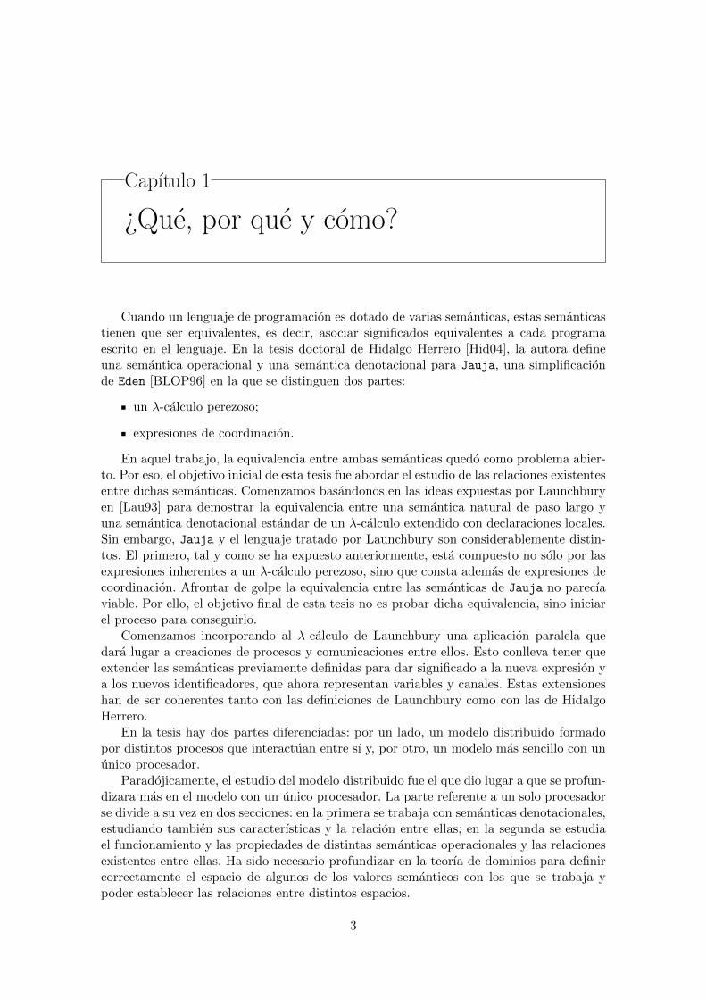
Cuando un lenguaje de programacion es dotado de varias semanticas, estas semanticastienen que ser equivalentes, es decir, asociar significados equivalentes a cada programaescrito en el lenguaje. En la tesis doctoral de Hidalgo Herrero [Hid04], la autora defineuna semantica operacional y una semantica denotacional para Jauja, una simplificacionde Eden [BLOP96] en la que se distinguen dos partes:
un λ-calculo perezoso;
expresiones de coordinacion.
En aquel trabajo, la equivalencia entre ambas semanticas quedo como problema abier-to. Por eso, el objetivo inicial de esta tesis fue abordar el estudio de las relaciones existentesentre dichas semanticas. Comenzamos basandonos en las ideas expuestas por Launchburyen [Lau93] para demostrar la equivalencia entre una semantica natural de paso largo yuna semantica denotacional estandar de un λ-calculo extendido con declaraciones locales.Sin embargo, Jauja y el lenguaje tratado por Launchbury son considerablemente distin-tos. El primero, tal y como se ha expuesto anteriormente, esta compuesto no solo por lasexpresiones inherentes a un λ-calculo perezoso, sino que consta ademas de expresiones decoordinacion. Afrontar de golpe la equivalencia entre las semanticas de Jauja no parecıaviable. Por ello, el objetivo final de esta tesis no es probar dicha equivalencia, sino iniciarel proceso para conseguirlo.
Comenzamos incorporando al λ-calculo de Launchbury una aplicacion paralela quedara lugar a creaciones de procesos y comunicaciones entre ellos. Esto conlleva tener queextender las semanticas previamente definidas para dar significado a la nueva expresion ya los nuevos identificadores, que ahora representan variables y canales. Estas extensioneshan de ser coherentes tanto con las definiciones de Launchbury como con las de HidalgoHerrero.
En la tesis hay dos partes diferenciadas: por un lado, un modelo distribuido formadopor distintos procesos que interactuan entre sı y, por otro, un modelo mas sencillo con ununico procesador.
Paradojicamente, el estudio del modelo distribuido fue el que dio lugar a que se profun-dizara mas en el modelo con un unico procesador. La parte referente a un solo procesadorse divide a su vez en dos secciones: en la primera se trabaja con semanticas denotacionales,estudiando tambien sus caracterısticas y la relacion entre ellas; en la segunda se estudiael funcionamiento y las propiedades de distintas semanticas operacionales y las relacionesexistentes entre ellas. Ha sido necesario profundizar en la teorıa de dominios para definircorrectamente el espacio de algunos de los valores semanticos con los que se trabaja ypoder establecer las relaciones entre distintos espacios.
3
4 Capıtulo 1. ¿Que, por que y como?
Como era de esperar, no han sido pocos los problemas que se han encontrado a lo largodel estudio, y a los que hemos tenido que dar solucion. Parte del trabajo realizado ha sidoconsecuencia de la ausencia de demostraciones detalladas para los resultados que propusoLaunchbury en [Lau93]. En dicho trabajo se exponen las ideas intuitivas sobre las quese han de construir las demostraciones, pero el desarrollo de las mismas es bastante mascomplicado de lo que se muestra en dicho artıculo y lo que en un primer momento pareceresolverse con una simple induccion por reglas ha resultado ser mucho mas complejo. Dadoque diversos trabajos [BKT00, HO02, NH09, Ses97, vEdM07] se basan en este estudio deLaunchbury, se ha considerado de gran importancia formalizar los resultados expuestos enel.
Por otra parte, la notacion con la que se representan las expresiones de los lenguajespuede facilitar o dificultar las demostraciones formales. En el caso del λ-calculo, es bastantefrecuente encontrar problemas relacionados con los nombres elegidos para expresar untermino, es decir, problemas derivados de la α-conversion. Se han desarrollado distintastecnicas para evitarlos, como por ejemplo la notacion de de Bruijn [dB72], la representacionlocalmente sin nombres [Cha11], o las tecnicas de la logica nominal [Pit13]. En nuestro casose ha elegido la segunda opcion, con la que hemos trabajado en algunos de los artıculosque componen esta tesis.
En resumen, la busqueda de la equivalencia entre las semanticas de un modelo dis-tribuido nos ha hecho adentrarnos y profundizar en distintas semanticas para un modelomas sencillo y en diversas tecnicas derivadas de notaciones alternativas para expresar losterminos del lenguaje.
1.1 Objetivos de la tesis
El objetivo principal de la tesis ha sido:
encauzar la demostracion de la equivalencia entre las semanticas definidas para Jauja
en [Hid04].
Dicho proposito ha quedado desglosado en los siguientes objetivos especıficos:
extender el λ-calculo con una aplicacion paralela, es decir, incluir en el lenguaje unoperador para introducir explıcitamente el paralelismo;
definir para este λ-calculo extendido distintos modelos semanticos con uno y convarios procesadores, tanto operacionales como denotacionales;
estudiar las relaciones entre los modelos semanticos definidos: formalizar la equiva-lencia entre las semanticas definidas en el paso anterior;
formalizar algunas de las demostraciones ausentes en [Lau93]: en concreto la equiva-lencia entre una semantica denotacional estandar y una de recursos y la equivalenciaentre la semantica natural definida por Launchbury y su version alternativa.
1.2 Organizacion de la tesis
Esta tesis se presenta como una coleccion de publicaciones ya realizadas. Para entenderla relacion entre los artıculos de esta coleccion y obtener una vision de conjunto, se hacompletado el trabajo con este capıtulo introductorio y tres capıtulos mas que se enume-ran a continuacion: en el Capıtulo 2 se explican los conceptos previos que se consideran
1.2. Organizacion de la tesis 5
necesarios para poder entender el estudio realizado. El Capıtulo 3 esta dedicado a los re-sultados obtenidos. Mas que detallar cada uno de ellos, lo que se ha hecho en las distintaspublicaciones, este capıtulo pretende dar una idea intuitiva de ellos de forma que facilitela lectura y comprension de los artıculos. Cada seccion del capıtulo esta ligada a una ovarias publicaciones que se indican explıcitamente. Tambien en este capıtulo se enumerany comentan algunos de los trabajos de otros autores relacionados con esta tesis. Por suparte, el trabajo futuro se desarrolla en el Capıtulo 4. Esta dividido en cuatro secciones yen ellas se indica si ya se ha realizado una parte de ese trabajo. Finalmente, el Capıtulo 5recoge las cuatro publicaciones principales que componen esta tesis:
P1: Relating function spaces to resourced function spaces [SGHHOM11].
P2: A Locally Nameless Representation for a Natural Semantics for Lazy Evalua-tion [SGHHOM12b].
P3: The Role of Indirections in Lazy Natural Semantics [SGHHOM14b].
P4: An Operational Semantics for Distributed Lazy Evaluation [SGHHOM10].
Ademas se han incluido dos apendices. El Apendice A contiene las versiones extendidasde las publicaciones P2 y P3. En dichas extensiones se detallan todas las demostracionesrealizadas para obtener los resultados expuestos en las publicaciones.
TR1: A locally nameless representation for a natural semantics for lazy evaluation(extended version) [SGHHOM12c].
TR2: The role of indirections in lazy natural semantics (extended version) [SGHHOM13].
Finalmente, el Apendice B esta formado por dos trabajos presentados en su momentocomo trabajo en progreso y cuyo desarrollo se ha postergado por diversas razones:
WP1: Launchbury’s semantics revisited: On the equivalence of context-heap seman-tics [SGHHOM14a].
WP2: A formalization in Coq of Launchbury’s natural semantics for lazy evalua-tion [SGHHOM12a].

6 Capıtulo 1. ¿Que, por que y como?
Capıtulo 2
¿Que estaba hecho?
En este capıtulo se repasan algunos conceptos que consideramos necesarios para en-tender la investigacion realizada en esta tesis.
2.1 Lenguajes de programacion
Todo lenguaje lleva asociado una sintaxis y una semantica. Segun la Real AcademiaEspanola [Esp14], la sintaxis es “el conjunto de reglas que definen las secuencias correctasde los elementos de un lenguaje”, mientras que la semantica es “el estudio del significadode los signos linguısticos y de sus combinaciones, desde un punto de vista sincronico odiacronico” (segun aparece en el avance de la vigesima tercera edicion). De manera infor-mal podemos decir que la sintaxis muestra como construir correctamente expresiones y lasemantica dota de significado a esos terminos bien construidos. Esto tambien es aplicablea los lenguajes de programacion, donde la sintaxis indica como construir programas y lasemantica indica como se comportaran esos programas al ser ejecutados en una compu-tadora.
A veces, en los lenguajes naturales encontramos oraciones cuyo significado no es uni-co. Por ejemplo: Ana cogio su bicicleta. Esta frase es ambigua, pues si Ana esta jugandocon Pablo en el parque no sabemos si ha cogido la bicicleta de Pablo o su propia bici-cleta. Sin embargo, los lenguajes de programacion vienen dotados de semanticas formalesque impiden la ambiguedad de sus significados: a cada termino le corresponde un unicosignificado.
2.1.1 Lenguajes de programacion funcionales
Existen diversos paradigmas de programacion. En el imperativo el programador definepaso a paso la solucion a un problema, alejandose de la definicion matematica inicial. Porcontra, los lenguajes funcionales elevan el nivel de abstraccion.
Consideremos por ejemplo como calcular la potencia n-esima de un numero. Su defi-nicion matematica podrıa ser la siguiente:
x0 = 1xn+1 = x · xn
En un lenguaje imperativo la expresion para la funcion potencia pierde su similitud
7

8 Capıtulo 2. ¿Que estaba hecho?
con la definicion anterior, como puede verse al implementarla en C:
int potencia(int x, int n);{
int i = 1;int resultado = 1;while (i <= n){
resultado = resultado ∗ x;i+ +;
}return(resultado);
}
Mientras que en un lenguaje funcional como Haskell, la implementacion quedarıa:
potencia x 0 = 1potencia x n = x ∗ potencia x (n− 1)
En muchas ocasiones se atribuye a los lenguajes funcionales una menor eficiencia en suejecucion. En la edicion revisada de [BB00], Barendregt y Barendsen explican que la ar-quitectura Von-Neumann se basa en la maquina de Turing. Los lenguajes de programacionimperativos siguen una secuencia de instrucciones que se ajusta a dicha arquitectura. Sinembargo, son las maquinas de reduccion las que se disenan para la ejecucion de lenguajesfuncionales basados en el λ-calculo. La mayor parte de las computadoras actuales tienenuna arquitectura Von-Neumann, dando lugar ciertamente a una menor eficiencia de loslenguajes funcionales. Por ese motivo, gran parte de la investigacion sobre lenguajes deprogramacion funcional se ha dedicado a la implementacion eficiente de estos lenguajes,habiendose alcanzado hoy en dıa unas velocidades de ejecucion verdaderamente competiti-vas. Esto, unido a las muchas ventajas que ofrecen los lenguajes funcionales desde el puntode vista del desarrollador (mayor nivel de abstraccion, codigo mas reducido, ausencia deefectos colaterales —transparencia referencial—, facil depuracion de programas, concu-rrencia, actualizaciones “en caliente” —hot code deployment—, recursion natural, etc),ha hecho florecer la programacion funcional en ambitos distintos del academico [OSV10].Por ejemplo, Haskell es utilizado por algunas empresas como Intel y algunos bancos comoDeutsche Bank; y ciertas partes de Facebook o Google estan programadas usando este len-guaje (una lista mas detallada puede encontrarse en [has14a]). Erlang tambien es utilizadoen la industria [erl14a], por ejemplo en Whatsapp [wha14], Facebook y T-Mobile [erl14b].
2.1.2 Estrategias de evaluacion
Las expresiones de los lenguajes de programacion funcionales se evaluan mediante lareduccion de subexpresiones. Dependiendo del orden de reduccion establecido para losredexes (expresiones de reduccion) se obtienen diferentes estrategias de evaluacion quepueden encuadrarse en dos grandes grupos: el primero esta formado por las estrategias enlas que la evaluacion de los argumentos se realiza antes de aplicar la funcion aunque nosean requeridos (evaluacion impaciente); el segundo, por aquellas en las que los argumentossolo se calculan cuando se necesitan sus resultados (evaluacion perezosa).
Existen numerosas estrategias de evaluacion, aunque aquı solo se detallan tres de ellas,por ser las que aparecen en el desarrollo de esta tesis: call-by-value, call-by-name y call-by-need. Segun las definiciones de Reade en [Rea89].
2.1. Lenguajes de programacion 9
Call-by-value: es una estrategia de evaluacion impaciente en la que los argumentosson evaluados por completo antes que el cuerpo de la funcion;
Call-by-name: en este caso el argumento (sin evaluar) es sustituido en el cuerpode la funcion y la expresion resultante es evaluada, tratandose, por tanto, de unaestrategia del segundo grupo. De esta forma es posible que algunas expresiones seanevaluadas mas de una vez, aunque si no son requeridas no se evaluaran nunca;
Call-by-need : es una estrategia de evaluacion perezosa mas eficiente que la estrategiaanterior, ya que una vez obtenido el valor de una expresion este se guarda y comparte,y ası no debe ser calculado de nuevo.
2.1.3 Lenguajes funcionales paralelos
La proliferacion de maquinas paralelas y distribuidas hace que surja la necesidad dedisenar lenguajes que faciliten la programacion paralela, y los lenguajes funcionales para-lelos ofrecen grandes ventajas para ello. Si bien los lenguajes imperativos son eficientes,tratan a un nivel de abstraccion muy bajo conceptos clave como la sincronizacion y lacomunicacion. Sin embargo, los lenguajes funcionales son una buena opcion debido a sualto nivel de abstraccion, a la transparencia referencial y a su modelo semantico claro(ventajas que ya han sido comentadas en la Seccion 2.1.1).
Loogen realiza una clasificacion del paralelismo en lenguajes funcionales en [Loo99]distinguiendo tres grandes grupos, dependiendo de la libertad que se deje al programadorpara establecer los puntos del programa susceptibles de ser evaluados en paralelo:
Paralelismo implıcito: es el inherente a la semantica de reduccion, donde los redexesindependientes pueden ser reducidos en un orden arbitrario o en paralelo. Es la basede la paralelizacion automatica de los lenguajes funcionales.
Paralelismo semi-explıcito: el programador indica donde desearıa una evaluacionen paralelo anadiendo anotaciones para el compilador. Bien se utilizan construc-ciones paralelas de alto nivel como esqueletos [Col89], bien estrategias de evalua-cion [THLP98]. Pero estas anotaciones podrıan ser ignoradas por el compilador.
Paralelismo explıcito: el programador establece donde computar distintas expresio-nes en paralelo. Existen extensiones de algunos lenguajes de programacion comoHaskell [Pey03] o ML [MTH90] con construcciones para la creacion explıcita deprocesos, la comunicacion de valores y la sincronizacion entre procesos.
El lenguaje funcional Haskell [Pey03, has14b] ha sido la base de numerosas versionesparalelas y distribuidas, como se senala en [TLP03]. La evaluacion en Haskell es perezosa(Seccion 2.1.2). Este tipo de evaluacion restringe la explotacion del paralelismo, pues lasexpresiones solo se evaluan bajo demanda. Por eso las versiones paralelas de Haskell tratande eliminar la pereza, ya sea mediante el trabajo especulativo, permitiendo la evaluacionde partes no demandadas (como por ejemplo en GpH [THLP98] con el operador par), obien introduciendo estrictez, al forzar la evaluacion de partes antes de que su resultadosea necesario (el operador seq en GpH [THLP98]).
2.1.4 El lenguaje funcional paralelo Eden
El lenguaje que ha inspirado los trabajos de esta tesis es Eden [BLOP96, LOP05, ede14],una extension de Haskell con construcciones de coordinacion para controlar la evaluacion
10 Capıtulo 2. ¿Que estaba hecho?
en paralelo. La coordinacion en Eden se basa en la definicion explıcita de procesos y enla comunicacion implıcita mediante streams. A continuacion, se resumen las principalescaracterısticas de Eden (segun se indica en [Hid04]):
Abstracciones de proceso: son las expresiones que de un modo puramente funcionaldefinen el comportamiento general de un proceso.
Creaciones de proceso: son aplicaciones de las anteriores a un grupo determinado deexpresiones que conformaran los valores de los canales de entrada del nuevo procesocreado.
Comunicaciones entre procesos: son asıncronas e implıcitas, pues el paso de mensajesno lo ha de explicitar el programador. Ademas, estas comunicaciones no tienen porque ser de un unico valor, sino que pueden realizarse en forma de streams.
Ademas, las construcciones de Eden se extienden para modelizar sistemas reactivos:
Creacion dinamica de canales: sin esta facilidad las comunicaciones son jerarquicasentre procesos padre y procesos hijo. Pero los canales dinamicos permiten romperesta jerarquıa, permitiendo topologıas de comunicacion mas complejas.
No-determinismo: para poder modelizar las comunicaciones de varios a uno, se in-troduce la abstraccion de proceso que toma varios streams devolviendo uno solo quees una mezcla no determinista de los elementos de los anteriores.
2.2 Semanticas de lenguajes de programacion
En el prefacio del texto de Winskel [Win93] se explica que dotar de una semanti-ca formal a un lenguaje de programacion consiste en construir un modelo matematico.Las semanticas formales permiten comprender y razonar sorbre el comportamiento de losprogramas.
2.2.1 Semanticas formales
Dependiendo del uso que se le quiera dar, se considerara un tipo de semantica formalu otro. Destacamos aquı los dos utilizados en esta tesis:
Operacional: la semantica operacional de un lenguaje describe el significado de unprograma especificando como se ejecuta en una maquina abstracta. Esta semanticase centra en conocer el resultado que genera un programa y el modo en que este esobtenido. Distinguimos dos categorıas: las semanticas de paso corto, que describencomo se realiza cada computacion paso a paso; y las semanticas de paso largo, onaturales, que describen como se obtiene directamente el resultado final.
Denotacional: la semantica denotacional dota de significado a los programas cons-truyendo unos objetos matematicos, llamados denotaciones, que describen el signi-ficado de las expresiones del lenguaje. Podrıamos decir que se trata de encontrarobjetos matematicos que representen lo que hace un programa. Una semantica de-notacional viene dada por la funcion que computa el programa, pero no se ocupa decomo se llega a ello. La denotacion de un termino se obtiene componiendo las denota-ciones de sus subterminos. Por tener un mayor nivel de abstraccion que la semanticaoperacional, permite estudiar mas facilmente la equivalencia entre programas. La

2.3. Espacios de funciones 11
forma usual de definir una semantica denotacional se centra en los siguientes as-pectos: definir el espacio de significados; dotar a cada constante del lenguaje de unsignificado en dicho espacio; construir funciones semanticas sobre el espacio de signi-ficados para cada operador del lenguaje; y, finalmente, definir la funcion semanticaprincipal que indica el valor semantico de cada programa.
Cuando hay mas de un tipo de semantica definida para el mismo lenguaje, hay quedemostrar que estas son equivalentes. En el caso de las semanticas operacionales y deno-tacionales, esta equivalencia suele darse en terminos de correccion y adecuacion compu-tacional:
Correccion: indica que las reducciones operacionales preservan el significado de-notacional de los terminos.
Adecuacion: la adecuacion computacional de una semantica operacional con res-pecto a una denotacional establece que si una expresion esta definida segun lasemantica denotacional, entonces existe una reduccion operacional para ella.
En esta tesis se trabaja con distintas semanticas operacionales y denotacionales paraun lenguaje de programacion funcional, y se estudian las relaciones existentes entre ellas.
2.3 Espacios de funciones
En algunas ocasiones, comparar programas que estan escritos en lenguajes de progra-macion diferentes puede ser bastante complicado si se utilizan semanticas operacionalescuyas transiciones se construyen a partir de la sintaxis del lenguaje, tal y como se explicaen [Win93]. Por ello surge la necesidad de dar significado a las expresiones de una formamas abstracta, mediante una semantica denotacional cuyos valores se encuentran en unespacio de funciones.
Abramsky y Jung en [AJ94] introducen los dos problemas que dan lugar a la teorıade dominios [Sco73]: el menor punto fijo como significado de definiciones recursivas y lasecuaciones de dominios recursivos. Asımismo, Abramsky en [Abr91] explica como la teorıade dominios, introducida por Scott, ha sido estudiada tanto desde el marco teorico comoaplicado, en particular al campo de las semanticas denotacionales.
2.3.1 Conceptos basicos
A continuacion, vamos a repasar algunos conceptos clave de la teorıa de dominios.Daremos sus definiciones siguiendo el texto de Winskel sobre semanticas formales paralenguajes de programacion [Win93].
Un conjunto P dotado de una operacion binaria, v, es un orden parcial si la relaciones reflexiva, transitiva y antisimetrica.
Dado un subconjunto X ⊆ P , p ∈ P es una cota superior de X si cualquier elementode X es menor o igual que p, es decir, ∀q ∈ X . q v p. Ademas, esta cota sera mınima(⊔X) si cualquier otra cota superior es mayor que ella.Un orden parcial (P,v) sera completo (cpo) si para toda cadena infinita creciente de
elementos (d0 v d1 v · · · v dn v . . . ) existe una cota superior mınima (⊔ndn) en P . Si
ademas esta dotado de un elemento mınimo (⊥), se dira que es un orden parcial completocon mınimo.
Dados dos cpos (D,vD) y (E,vE), una funcion f : D → E es monotona si ∀d, d′ ∈D . d vD d′ ⇒ f(d) vE f(d′). Ademas, sera continua si es monotona y para cada
12 Capıtulo 2. ¿Que estaba hecho?
cadena infinita (d0 v d1 v · · · v dn v . . . ) se cumple que la cota superior mınima de lasimagenes coincide con la imagen de la cota superior mınima de los elementos, es decir,⊔E
nf(dn) = f(
⊔D
ndn).
Dado un cpo (D,vD) y una funcion continua f : D → D, se dice que un elementod ∈ D es un punto fijo de f si f(d) = d.
Teorema de Kleene del punto fijo. Sea (D,vD) un cpo con mınimo y f : D → Duna funcion continua. Se define fix(f) =
⊔nfn(⊥). Se verifica que
1. fix(f) es un punto fijo de f , es decir, f(fix(f)) = fix(f);
2. Si f(d) = d entonces fix(f) v d.
Luego fix(f) es el menor punto fijo de f .
Dados dos cpos (D,vD) y (E,vE), el espacio de funciones [D → E] consiste en los
elementos {f | f : D → E es continua} ordenados punto a punto mediante f v gdef=
∀d ∈ D.f(d) v g(d). Esto hace que el espacio de funciones sea un cpo y para cada cadenainfinita f0 v f1 v · · · v fn v . . . la cota superior mınima cumple: (
⊔nfn)d =
⊔n
(fn(d)).
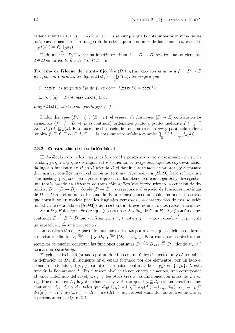
2.3.2 Construccion de la solucion inicial
El λ-calculo puro y los lenguajes funcionales perezosos no se corresponden en su to-talidad, ya que hay que distinguir entre elementos convergentes, aquellos cuya evaluacionda lugar a funciones de D en D (siendo D el dominio adecuado de valores), y elementosdivergentes, aquellos cuya evaluacion no termina. Abramsky en [Abr90] hace referencia aeste hecho y propone, para poder representar los elementos convergentes y divergentes,una teorıa basada en sistemas de transicion aplicativos, introduciendo la ecuacion de do-minios, D = [D → D]⊥, donde [D → D]⊥ corresponde al espacio de funciones continuasde D en D con el mınimo (⊥) anadido. Esta ecuacion tiene una solucion inicial no trivialque constituye un modelo para los lenguajes perezosos. La construccion de esta solucioninicial viene detallada en [AO93] y aquı se hara un breve resumen de los pasos principales.
Sean D y E dos cpos. Se dice que 〈i, j〉 es un embedding de D en E si i y j son funciones
continuas Di� E
j� D que verifican que i ◦ j v idE y j ◦ i = idD, donde
i� representa
un inyeccion yj� una proyeccion.
La construccion del espacio de funciones se realiza por niveles, que se definen de forma
recursiva mediante D0def= {⊥} y Dn+1
def= [Dn → Dn]⊥. Para cada par de niveles con-
secutivos se pueden construir las funciones continuas Dnin� Dn+1
jn� Dn, donde 〈in, jn〉forman un embedding.
El primer nivel esta formado por un dominio con un unico elemento, tal y como indicala definicion de D0. El siguiente nivel estara formado por dos elementos, por un lado elelemento indefinido, ⊥D1 , y por otro la funcion continua de {⊥D0} en {⊥D0}. A estafuncion la llamaremos d1. En el tercer nivel se tienen cuatro elementos, uno correspondeal valor indefinido del nivel, ⊥D2 , y los otros tres a las funciones continuas de D1 enD1. Puesto que en D1 hay dos elementos y verifican que ⊥D1v d1, existen tres funcionescontinuas: d20, d21 y d22 tales que d20(⊥D1) =⊥D1v d20(d1) =⊥D1 , d21(⊥D1) =⊥D1vd21(d1) = d1 y d22(⊥D1) = d1 v d22(d1) = d1, respectivamente. Estos tres niveles serepresentan en la Figura 2.1.

2.3. Espacios de funciones 13
⊥D0
D0
D0 D0
D1
⊥D1
d1
D2
⊥D2
d21
d20
d22
Figura 2.1: Primeros niveles del espacio de funciones [D → D]⊥
...
...
Dn
⊥Dn
...
Dk
⊥Dk
iknjnk
Figura 2.2: Inyecciones y proyecciones entre niveles
Existe una generalizacion de los embeddings, de forma que se puede pasar del nivelk al nivel n mediante la inyeccion ikn y la proyeccion jnk. Sin embargo, estas funcionesno son exactamente inversas. Cuando pasamos de un nivel a otro superior mediante unainyeccion, se busca un valor de ese nivel cuya proyeccion corresponda al valor de inicio.Ahora bien, en ese nivel superior se dispone de mas informacion, ası que habra mas de unvalor que cumpla el requisito; de entre todos ellos se elige el mas indefinido. Por lo tanto,ikn ◦ jnk v idn y jnk ◦ ikn = idk, propiedad que viene heredada de los embeddings entreniveles consecutivos. La Figura 2.2 muestra esta situacion para n > k.
Notese que 〈Dn, jn〉n∈ω es un sistema inverso de cpo’s. D esta definido como el lımiteinverso del sistema anterior, es decir, D = lım←〈Dn, jn〉n∈ω y la solucion inicial se identi-fica con D = {〈xn : n ∈ ω〉 : xn ∈ Dn ∧ jn(xn+1) = xn}. Se denota por ψn a la proyeccionj∞n : D�Dn y por φn a la inyeccion in∞ : Dn�D. Tal y como explica Abramsky yOng [AO93] se considera Dn como un subconjunto de D, es decir, si x ∈ Dn entonces seidentifica φn(x) con x, y si x ∈ D entonces ψn(x) se identifica con xn ∈ Dn. Por lo queD =
⋃nDn. Los valores denotacionales para el λ-calculo estan definidos sobre el dominio
D = [D → D]⊥.
14 Capıtulo 2. ¿Que estaba hecho?
λx.P ⇓ λx.PM ⇓ λx.P P [x := Q] ⇓ N
M Q ⇓ N
Figura 2.3: Relacion binaria en Λ0
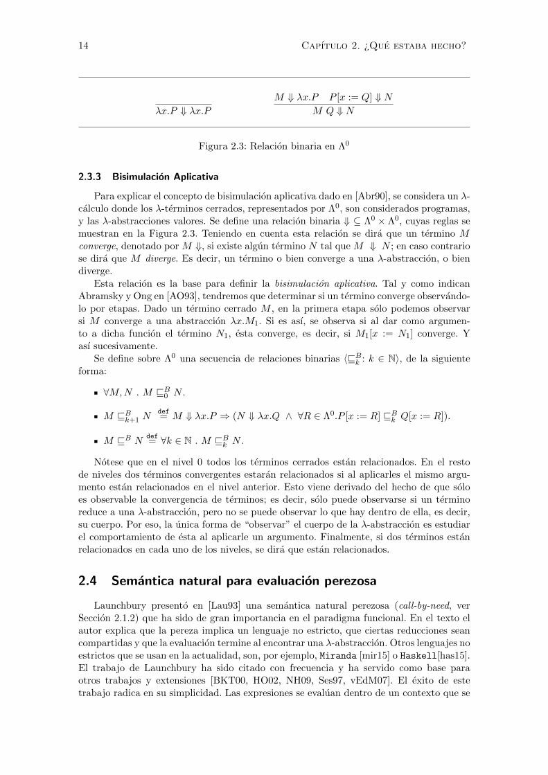
2.3.3 Bisimulacion Aplicativa
Para explicar el concepto de bisimulacion aplicativa dado en [Abr90], se considera un λ-calculo donde los λ-terminos cerrados, representados por Λ0, son considerados programas,y las λ-abstracciones valores. Se define una relacion binaria ⇓ ⊆ Λ0 × Λ0, cuyas reglas semuestran en la Figura 2.3. Teniendo en cuenta esta relacion se dira que un termino Mconverge, denotado por M ⇓, si existe algun termino N tal que M ⇓ N ; en caso contrariose dira que M diverge. Es decir, un termino o bien converge a una λ-abstraccion, o biendiverge.
Esta relacion es la base para definir la bisimulacion aplicativa. Tal y como indicanAbramsky y Ong en [AO93], tendremos que determinar si un termino converge observando-lo por etapas. Dado un termino cerrado M , en la primera etapa solo podemos observarsi M converge a una abstraccion λx.M1. Si es ası, se observa si al dar como argumen-to a dicha funcion el termino N1, esta converge, es decir, si M1[x := N1] converge. Yası sucesivamente.
Se define sobre Λ0 una secuencia de relaciones binarias 〈vBk : k ∈ N〉, de la siguienteforma:
∀M,N . M vB0 N .
M vBk+1 Ndef= M ⇓ λx.P ⇒ (N ⇓ λx.Q ∧ ∀R ∈ Λ0.P [x := R] vBk Q[x := R]).
M vB Ndef= ∀k ∈ N . M vBk N .
Notese que en el nivel 0 todos los terminos cerrados estan relacionados. En el restode niveles dos terminos convergentes estaran relacionados si al aplicarles el mismo argu-mento estan relacionados en el nivel anterior. Esto viene derivado del hecho de que soloes observable la convergencia de terminos; es decir, solo puede observarse si un terminoreduce a una λ-abstraccion, pero no se puede observar lo que hay dentro de ella, es decir,su cuerpo. Por eso, la unica forma de “observar” el cuerpo de la λ-abstraccion es estudiarel comportamiento de esta al aplicarle un argumento. Finalmente, si dos terminos estanrelacionados en cada uno de los niveles, se dira que estan relacionados.
2.4 Semantica natural para evaluacion perezosa
Launchbury presento en [Lau93] una semantica natural perezosa (call-by-need, verSeccion 2.1.2) que ha sido de gran importancia en el paradigma funcional. En el texto elautor explica que la pereza implica un lenguaje no estricto, que ciertas reducciones seancompartidas y que la evaluacion termine al encontrar una λ-abstraccion. Otros lenguajes noestrictos que se usan en la actualidad, son, por ejemplo, Miranda [mir15] o Haskell[has15].El trabajo de Launchbury ha sido citado con frecuencia y ha servido como base paraotros trabajos y extensiones [BKT00, HO02, NH09, Ses97, vEdM07]. El exito de estetrabajo radica en su simplicidad. Las expresiones se evaluan dentro de un contexto que se
2.4. Semantica natural para evaluacion perezosa 15
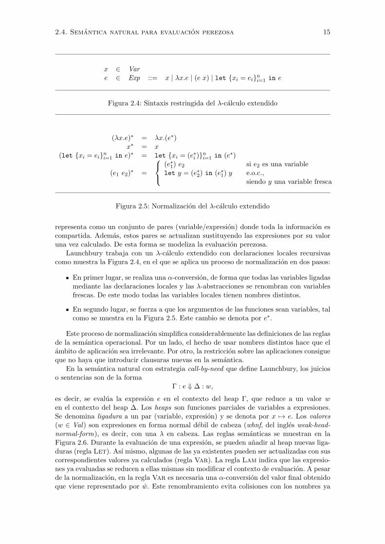
x ∈ Vare ∈ Exp ::= x | λx.e | (e x) | let {xi = ei}ni=1 in e
Figura 2.4: Sintaxis restringida del λ-calculo extendido
(λx.e)∗ = λx.(e∗)x∗ = x
(let {xi = ei}ni=1 in e)∗ = let {xi = (e∗i )}ni=1 in (e∗)
(e1 e2)∗ =
(e∗1) e2 si e2 es una variablelet y = (e∗2) in (e∗1) y e.o.c.,
siendo y una variable fresca
Figura 2.5: Normalizacion del λ-calculo extendido
representa como un conjunto de pares (variable/expresion) donde toda la informacion escompartida. Ademas, estos pares se actualizan sustituyendo las expresiones por su valoruna vez calculado. De esta forma se modeliza la evaluacion perezosa.
Launchbury trabaja con un λ-calculo extendido con declaraciones locales recursivascomo muestra la Figura 2.4, en el que se aplica un proceso de normalizacion en dos pasos:
En primer lugar, se realiza una α-conversion, de forma que todas las variables ligadasmediante las declaraciones locales y las λ-abstracciones se renombran con variablesfrescas. De este modo todas las variables locales tienen nombres distintos.
En segundo lugar, se fuerza a que los argumentos de las funciones sean variables, talcomo se muestra en la Figura 2.5. Este cambio se denota por e∗.
Este proceso de normalizacion simplifica considerablemente las definiciones de las reglasde la semantica operacional. Por un lado, el hecho de usar nombres distintos hace que elambito de aplicacion sea irrelevante. Por otro, la restriccion sobre las aplicaciones consigueque no haya que introducir clausuras nuevas en la semantica.
En la semantica natural con estrategia call-by-need que define Launchbury, los juicioso sentencias son de la forma
Γ : e ⇓ ∆ : w,
es decir, se evalua la expresion e en el contexto del heap Γ, que reduce a un valor wen el contexto del heap ∆. Los heaps son funciones parciales de variables a expresiones.Se denomina ligadura a un par (variable, expresion) y se denota por x 7→ e. Los valores(w ∈ Val) son expresiones en forma normal debil de cabeza (whnf, del ingles weak-head-normal-form), es decir, con una λ en cabeza. Las reglas semanticas se muestran en laFigura 2.6. Durante la evaluacion de una expresion, se pueden anadir al heap nuevas liga-duras (regla Let). Ası mismo, algunas de las ya existentes pueden ser actualizadas con suscorrespondientes valores ya calculados (regla Var). La regla Lam indica que las expresio-nes ya evaluadas se reducen a ellas mismas sin modificar el contexto de evaluacion. A pesarde la normalizacion, en la regla Var es necesaria una α-conversion del valor final obtenidoque viene representado por w. Este renombramiento evita colisiones con los nombres ya

16 Capıtulo 2. ¿Que estaba hecho?
Lam Γ : λx.e ⇓ Γ : λx.e AppΓ : e ⇓ Θ : λy.e′ Θ : e′[x/y] ⇓ ∆ : w
Γ : (e x) ⇓ ∆ : w
VarΓ : e ⇓ ∆ : w
(Γ, x 7→ e) : x ⇓ (∆, x 7→ w) : wLet
(Γ, {xi 7→ ei}ni=1) : e ⇓ ∆ : w
Γ : let {xi = ei}ni=1 in e ⇓ ∆ : w
Figura 2.6: Semantica natural
[[λx.e]]ρ = Fn(λν.[[e]]ρt{x 7→ν})
[[e x]]ρ = ([[e]]ρ)↓Fn ([[x]]ρ)[[x]]ρ = ρ(x)
[[let x1 = e1 . . . xn = en in e]]ρ = [[e]]{{x1 7→e1...xn 7→en}}ρ
Figura 2.7: Semantica denotacional
existentes y se justifica por la convencion de variables de Barendregt [Bar84]. La regla Appreduce primero el termino e y tras obtener un valor (es decir, una λ-abstraccion) realizala aplicacion mediante una β-reduccion, evaluando la expresion resultante. Por ultimo, laregla Let, ademas de introducir en el heap las declaraciones locales, evalua el cuerpo dela expresion. Notese que debido a la normalizacion realizada previamente no puede haberconflictos entre las variables cuando estas son introducidas en el heap.
A su vez, Launchbury tambien doto de significado denotacional a las expresiones delλ-calculo basandose en el modelo de Abramsky [Abr90]. La funcion semantica de la queparte es la siguiente:
[[−]] : Exp → Env → Value
donde Exp representa las expresiones del λ-calculo (Figura 2.4), Value un dominio apro-piado que satisface la ecuacion Value = [Value → Value]⊥ (explicado en la Seccion 2.3), yEnv contiene los entornos de evaluacion de las variables libres. Los entornos son funcionesde variables a valores, es decir,
ρ ∈ Env = Var → Value.
La funcion semantica se incluye en la Figura 2.7, donde se utiliza una funcion que relacionalos heaps con los entornos:
{{−}} : Heap → Env → Env
Esta funcion captura la recursion generada por las declaraciones locales y viene definidapor:
{{x1 7→ e1 . . . xn 7→ en}}ρ = µρ′.ρ t (x1 7→ [[e1]]ρ′ . . . xn 7→ [[en]]ρ′)
En esta definicion el operador de menor punto fijo viene representado por µ. Esta funcionpuede verse como un modificador de entornos que solo cobra sentido si los entornos ylos heaps son consistentes; es decir, siempre que una variable aparezca ligada tanto en elentorno como en el heap, entonces estara ligada a valores para los que exista una cotasuperior.
2.4. Semantica natural para evaluacion perezosa 17
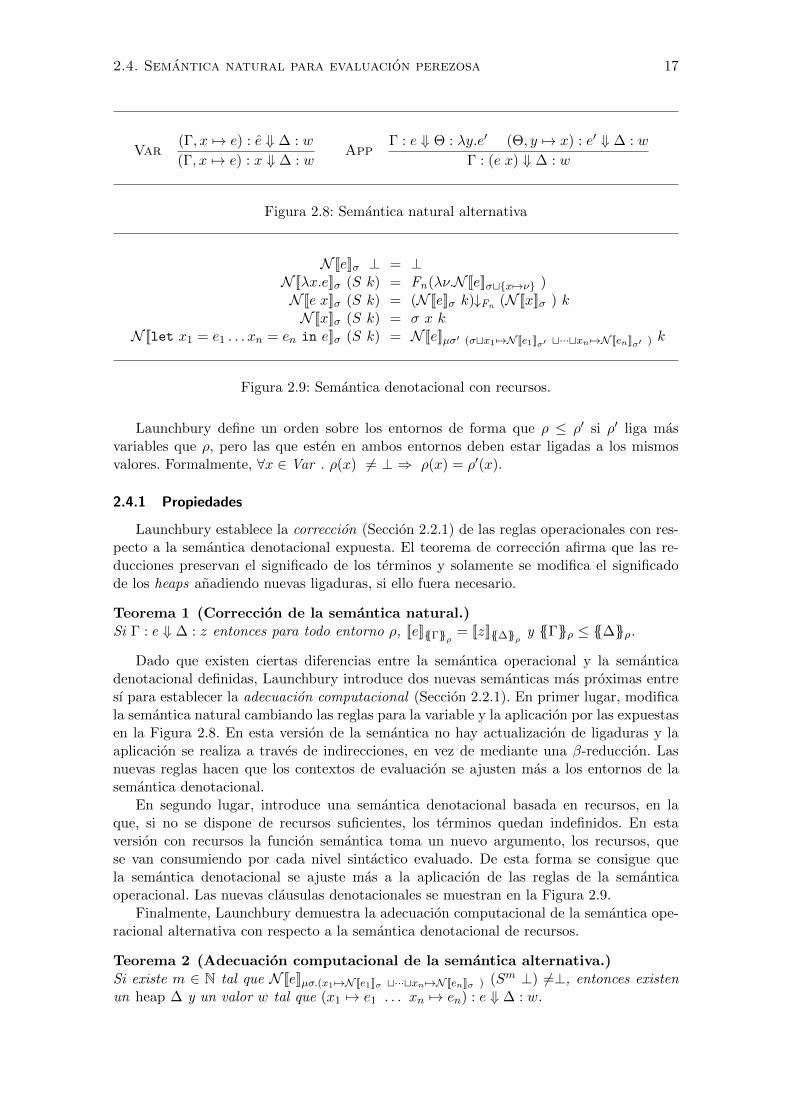
Var(Γ, x 7→ e) : e ⇓ ∆ : w
(Γ, x 7→ e) : x ⇓ ∆ : wApp
Γ : e ⇓ Θ : λy.e′ (Θ, y 7→ x) : e′ ⇓ ∆ : w
Γ : (e x) ⇓ ∆ : w
Figura 2.8: Semantica natural alternativa
N [[e]]σ ⊥ = ⊥N [[λx.e]]σ (S k) = Fn(λν.N [[e]]σt{x 7→ν} )
N [[e x]]σ (S k) = (N [[e]]σ k)↓Fn (N [[x]]σ ) kN [[x]]σ (S k) = σ x k
N [[let x1 = e1 . . . xn = en in e]]σ (S k) = N [[e]]µσ′ (σtx1 7→N [[e1]]σ′ t···txn 7→N [[en]]σ′ ) k
Figura 2.9: Semantica denotacional con recursos.
Launchbury define un orden sobre los entornos de forma que ρ ≤ ρ′ si ρ′ liga masvariables que ρ, pero las que esten en ambos entornos deben estar ligadas a los mismosvalores. Formalmente, ∀x ∈ Var . ρ(x) 6= ⊥ ⇒ ρ(x) = ρ′(x).
2.4.1 Propiedades
Launchbury establece la correccion (Seccion 2.2.1) de las reglas operacionales con res-pecto a la semantica denotacional expuesta. El teorema de correccion afirma que las re-ducciones preservan el significado de los terminos y solamente se modifica el significadode los heaps anadiendo nuevas ligaduras, si ello fuera necesario.
Teorema 1 (Correccion de la semantica natural.)Si Γ : e ⇓ ∆ : z entonces para todo entorno ρ, [[e]]{{Γ}}ρ = [[z]]{{∆}}ρ y {{Γ}}ρ ≤ {{∆}}ρ.
Dado que existen ciertas diferencias entre la semantica operacional y la semanticadenotacional definidas, Launchbury introduce dos nuevas semanticas mas proximas entresı para establecer la adecuacion computacional (Seccion 2.2.1). En primer lugar, modificala semantica natural cambiando las reglas para la variable y la aplicacion por las expuestasen la Figura 2.8. En esta version de la semantica no hay actualizacion de ligaduras y laaplicacion se realiza a traves de indirecciones, en vez de mediante una β-reduccion. Lasnuevas reglas hacen que los contextos de evaluacion se ajusten mas a los entornos de lasemantica denotacional.
En segundo lugar, introduce una semantica denotacional basada en recursos, en laque, si no se dispone de recursos suficientes, los terminos quedan indefinidos. En estaversion con recursos la funcion semantica toma un nuevo argumento, los recursos, quese van consumiendo por cada nivel sintactico evaluado. De esta forma se consigue quela semantica denotacional se ajuste mas a la aplicacion de las reglas de la semanticaoperacional. Las nuevas clausulas denotacionales se muestran en la Figura 2.9.
Finalmente, Launchbury demuestra la adecuacion computacional de la semantica ope-racional alternativa con respecto a la semantica denotacional de recursos.
Teorema 2 (Adecuacion computacional de la semantica alternativa.)Si existe m ∈ N tal que N [[e]]µσ.(x1 7→N [[e1]]σ t···txn 7→N [[en]]σ ) (Sm ⊥) 6=⊥, entonces existenun heap ∆ y un valor w tal que (x1 7→ e1 . . . xn 7→ en) : e ⇓ ∆ : w.
18 Capıtulo 2. ¿Que estaba hecho?
E ::= x | \x.E | E1 E2 | E1#E2 | let {xi = Ei}ni=1 in E| new(y, x)E | x ! E1 par E2 | E1 ./ E2 | Λ[x1 : x2].E1dcE2 | L
L ::= nil | [E1 : E2]
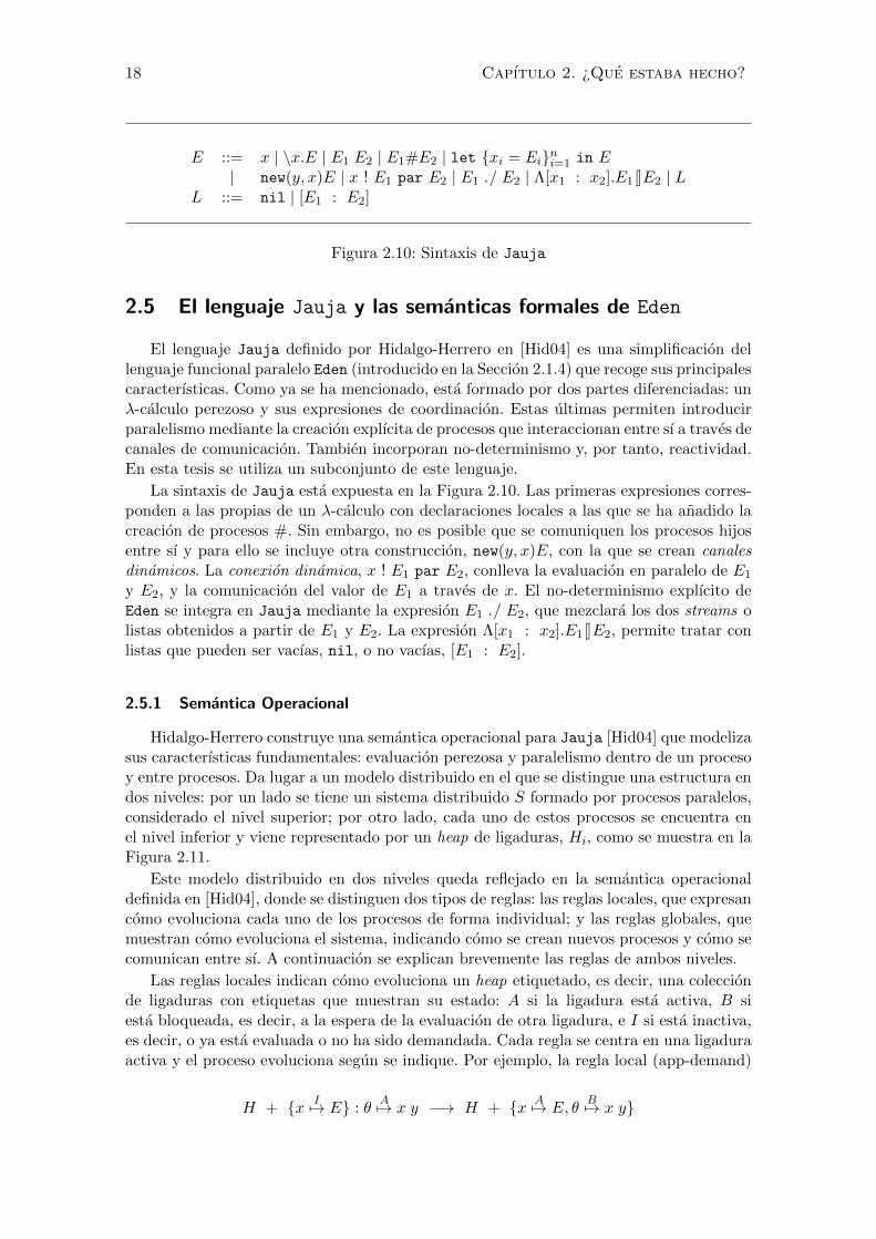
Figura 2.10: Sintaxis de Jauja
2.5 El lenguaje Jauja y las semanticas formales de Eden
El lenguaje Jauja definido por Hidalgo-Herrero en [Hid04] es una simplificacion dellenguaje funcional paralelo Eden (introducido en la Seccion 2.1.4) que recoge sus principalescaracterısticas. Como ya se ha mencionado, esta formado por dos partes diferenciadas: unλ-calculo perezoso y sus expresiones de coordinacion. Estas ultimas permiten introducirparalelismo mediante la creacion explıcita de procesos que interaccionan entre sı a traves decanales de comunicacion. Tambien incorporan no-determinismo y, por tanto, reactividad.En esta tesis se utiliza un subconjunto de este lenguaje.
La sintaxis de Jauja esta expuesta en la Figura 2.10. Las primeras expresiones corres-ponden a las propias de un λ-calculo con declaraciones locales a las que se ha anadido lacreacion de procesos #. Sin embargo, no es posible que se comuniquen los procesos hijosentre sı y para ello se incluye otra construccion, new(y, x)E, con la que se crean canalesdinamicos. La conexion dinamica, x ! E1 par E2, conlleva la evaluacion en paralelo de E1
y E2, y la comunicacion del valor de E1 a traves de x. El no-determinismo explıcito deEden se integra en Jauja mediante la expresion E1 ./ E2, que mezclara los dos streams olistas obtenidos a partir de E1 y E2. La expresion Λ[x1 : x2].E1dcE2, permite tratar conlistas que pueden ser vacıas, nil, o no vacıas, [E1 : E2].
2.5.1 Semantica Operacional
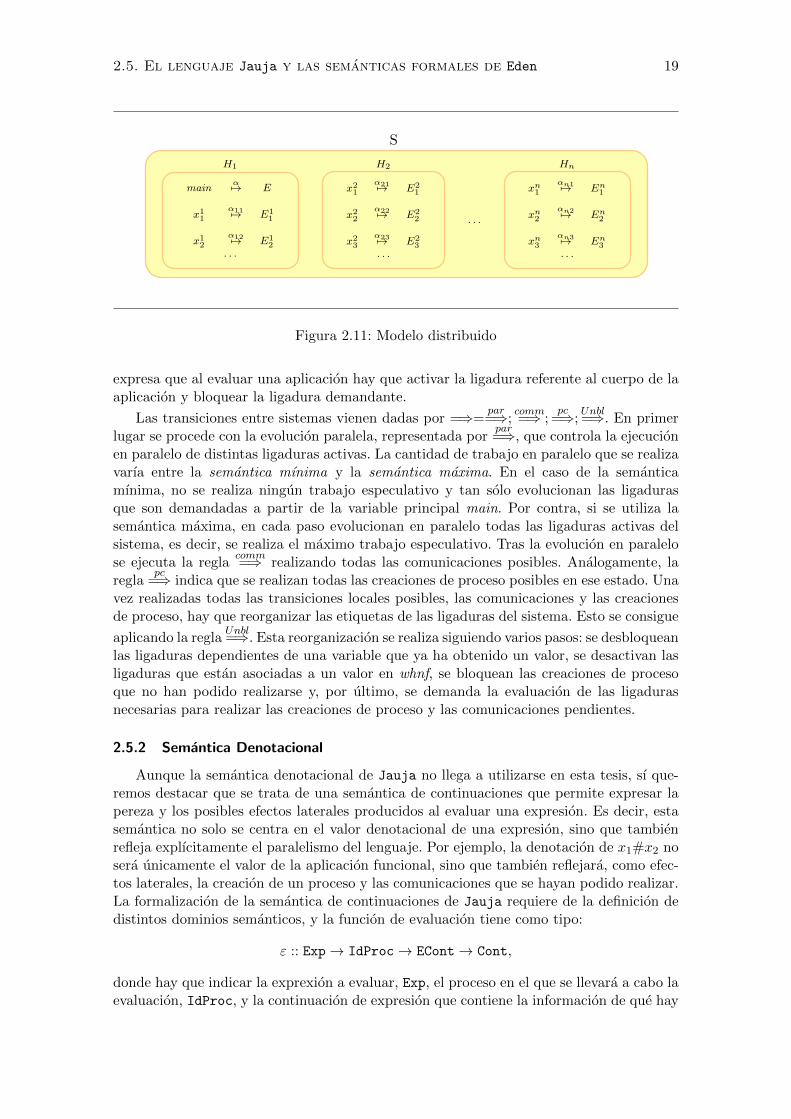
Hidalgo-Herrero construye una semantica operacional para Jauja [Hid04] que modelizasus caracterısticas fundamentales: evaluacion perezosa y paralelismo dentro de un procesoy entre procesos. Da lugar a un modelo distribuido en el que se distingue una estructura endos niveles: por un lado se tiene un sistema distribuido S formado por procesos paralelos,considerado el nivel superior; por otro lado, cada uno de estos procesos se encuentra enel nivel inferior y viene representado por un heap de ligaduras, Hi, como se muestra en laFigura 2.11.
Este modelo distribuido en dos niveles queda reflejado en la semantica operacionaldefinida en [Hid04], donde se distinguen dos tipos de reglas: las reglas locales, que expresancomo evoluciona cada uno de los procesos de forma individual; y las reglas globales, quemuestran como evoluciona el sistema, indicando como se crean nuevos procesos y como secomunican entre sı. A continuacion se explican brevemente las reglas de ambos niveles.
Las reglas locales indican como evoluciona un heap etiquetado, es decir, una coleccionde ligaduras con etiquetas que muestran su estado: A si la ligadura esta activa, B siesta bloqueada, es decir, a la espera de la evaluacion de otra ligadura, e I si esta inactiva,es decir, o ya esta evaluada o no ha sido demandada. Cada regla se centra en una ligaduraactiva y el proceso evoluciona segun se indique. Por ejemplo, la regla local (app-demand)
H + {x I7→ E} : θA7→ x y −→ H + {x A7→ E, θ
B7→ x y}
2.5. El lenguaje Jauja y las semanticas formales de Eden 19
S
H1 H2 Hn
mainα7→ E
x11
α117→ E11
x12
α127→ E12
. . .
x21
α217→ E21
x22
α227→ E22
x23
α237→ E23
. . .
. . .
xn1
αn17→ En
1
xn2
αn27→ En
2
xn3
αn37→ En
3
. . .
Figura 2.11: Modelo distribuido
expresa que al evaluar una aplicacion hay que activar la ligadura referente al cuerpo de laaplicacion y bloquear la ligadura demandante.
Las transiciones entre sistemas vienen dadas por =⇒=par=⇒;
comm=⇒ ;
pc=⇒;
Unbl=⇒. En primer
lugar se procede con la evolucion paralela, representada porpar=⇒, que controla la ejecucion
en paralelo de distintas ligaduras activas. La cantidad de trabajo en paralelo que se realizavarıa entre la semantica mınima y la semantica maxima. En el caso de la semanticamınima, no se realiza ningun trabajo especulativo y tan solo evolucionan las ligadurasque son demandadas a partir de la variable principal main. Por contra, si se utiliza lasemantica maxima, en cada paso evolucionan en paralelo todas las ligaduras activas delsistema, es decir, se realiza el maximo trabajo especulativo. Tras la evolucion en paralelose ejecuta la regla
comm=⇒ realizando todas las comunicaciones posibles. Analogamente, la
reglapc
=⇒ indica que se realizan todas las creaciones de proceso posibles en ese estado. Unavez realizadas todas las transiciones locales posibles, las comunicaciones y las creacionesde proceso, hay que reorganizar las etiquetas de las ligaduras del sistema. Esto se consigue
aplicando la reglaUnbl=⇒. Esta reorganizacion se realiza siguiendo varios pasos: se desbloquean
las ligaduras dependientes de una variable que ya ha obtenido un valor, se desactivan lasligaduras que estan asociadas a un valor en whnf, se bloquean las creaciones de procesoque no han podido realizarse y, por ultimo, se demanda la evaluacion de las ligadurasnecesarias para realizar las creaciones de proceso y las comunicaciones pendientes.
2.5.2 Semantica Denotacional
Aunque la semantica denotacional de Jauja no llega a utilizarse en esta tesis, sı que-remos destacar que se trata de una semantica de continuaciones que permite expresar lapereza y los posibles efectos laterales producidos al evaluar una expresion. Es decir, estasemantica no solo se centra en el valor denotacional de una expresion, sino que tambienrefleja explıcitamente el paralelismo del lenguaje. Por ejemplo, la denotacion de x1#x2 nosera unicamente el valor de la aplicacion funcional, sino que tambien reflejara, como efec-tos laterales, la creacion de un proceso y las comunicaciones que se hayan podido realizar.La formalizacion de la semantica de continuaciones de Jauja requiere de la definicion dedistintos dominios semanticos, y la funcion de evaluacion tiene como tipo:
ε :: Exp→ IdProc→ ECont→ Cont,
donde hay que indicar la exprexion a evaluar, Exp, el proceso en el que se llevara a cabo laevaluacion, IdProc, y la continuacion de expresion que contiene la informacion de que hay
20 Capıtulo 2. ¿Que estaba hecho?
que hacer con el valor obtenido, ECont. La funcion de evaluacion devolvera una continua-cion, Cont, que acumula los efectos de evaluar la expresion y los de la continuacion deexpresion.
2.6 Representaciones del λ-calculo
Tal y como explica Pitts en [Pit13], al definir un lenguaje de programacion se especifi-ca una sintaxis muy concreta que servira para generar los terminos (cadenas de sımbolos)correctos del lenguaje. Pero muchos detalles de esta sintaxis son irrelevantes para el sig-nificado de los programas.
Esta seccion se centra en el problema de la α-conversion generado por la sintaxis delλ-calculo. Uno de los problemas principales que surgen es la captura de variables libres ala hora de realizar una sustitucion. Por ello, siempre se habla de terminos α-equivalentes,que son aquellos que solo difieren en el nombre de las variables ligadas. Al realizar unademostracion formal, en el caso de que los nombres elegidos generen problemas (captura denombres), se puede cambiar el termino por otro α-equivalente, de modo que las variablesligadas del nuevo termino no causen problemas con las variables libres que aparecen en elresto de la demostracion. Esta forma de proceder es lo que se conoce como la convencionde variables de Barendregt [Bar84].
Sin embargo, y aunque durante muchos anos se ha utilizado sin mucha cautela, losnombres elegidos no son tan arbitrarios como se pretendıa y, por tanto, la convencionde Barendregt no siempre es aplicable, tal y como se explica en [UBN07]. Esto ocurrecon cierta frecuencia en pasos de demostraciones por induccion, donde el paso en cuestionpuede probarse para variables suficientemente frescas, pero no para una variable arbitrariacualquiera.
A continuacion, se exponen distintas alternativas al uso de la notacion con nombres.
2.6.1 Notacion de de Bruijn
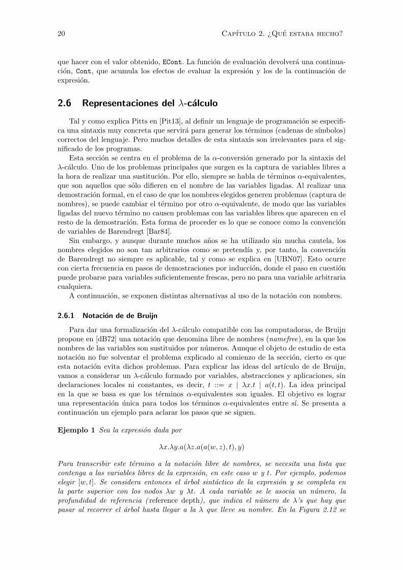
Para dar una formalizacion del λ-calculo compatible con las computadoras, de Bruijnpropone en [dB72] una notacion que denomina libre de nombres (namefree), en la que losnombres de las variables son sustituidos por numeros. Aunque el objeto de estudio de estanotacion no fue solventar el problema explicado al comienzo de la seccion, cierto es queesta notacion evita dichos problemas. Para explicar las ideas del artıculo de de Bruijn,vamos a considerar un λ-calculo formado por variables, abstracciones y aplicaciones, sindeclaraciones locales ni constantes, es decir, t ::= x | λx.t | a(t, t). La idea principalen la que se basa es que los terminos α-equivalentes son iguales. El objetivo es lograruna representacion unica para todos los terminos α-equivalentes entre sı. Se presenta acontinuacion un ejemplo para aclarar los pasos que se siguen.
Ejemplo 1 Sea la expresion dada por
λx.λy.a(λz.a(a(w, z), t), y)
Para transcribir este termino a la notacion libre de nombres, se necesita una lista quecontenga a las variables libres de la expresion, en este caso w y t. Por ejemplo, podemoselegir [w, t]. Se considera entonces el arbol sintactico de la expresion y se completa enla parte superior con los nodos λw y λt. A cada variable se le asocia un numero, laprofundidad de referencia ( reference depth), que indica el numero de λ’s que hay quepasar al recorrer el arbol hasta llegar a la λ que lleve su nombre. En la Figura 2.12 se
2.6. Representaciones del λ-calculo 21
w z
a t
a
λz y
a
λy
λx
λt
λw
5 1
4
1
Figura 2.12: Ejemplo de de Bruijn
muestra la construccion del arbol y la profundidad de referencia de cada variable. Ademasse han marcado con distinto color (marron) los nodos referentes a las variables libres.
Finalmente se sustituyen los nombres de las variables por los numeros obtenidos. Deeste modo la expresion dada con notacion libre de nombres sera λ.λ.a(λ.a(a(5, 1), 4), 1).
ut
Pero esta notacion libre de nombres tiene una gran desventaja, tal y como indica elpropio de Bruijn. Pese a su gran utilidad para trabajar en computadoras, resulta pocointuitiva y nada sencilla de usar para el ser humano. Por ejemplo, cada vez que se ejecutauna aplicacion, desaparece una λ del arbol sintactico y hay que recalcular los ındices de lasvariables. Desde el punto de vista de la maquina, esto no es complicado, pues se trata deaplicar ciertas reglas para el ajuste de ındices. Sin embargo, si se desea trabajar de formaabstracta sin terminos concretos, estos cambios complican considerablemente la sintaxisde la expresion.
2.6.2 Representacion localmente sin nombres
Para resolver los problemas derivados de la α-conversion, en esta tesis hemos optado porla representacion localmente sin nombres (locally nameless representation). Esta notacionfue tambien introducida por de Bruijn [dB72] como alternativa a la notacion expuesta en laSeccion 2.6.1. Consiste en utilizar ındices para las variables ligadas y mantener los nombresde las variables libres. Aunque esta notacion se ha utilizado en otros estudios [Gor94, Ler07,ACP+08], destaca el trabajo de Chargueraud [Cha11], que desarrolla una descripcioncompleta de esta representacion. En dicho trabajo se muestra la sintaxis del λ-calculoutilizando esta notacion, tal y como se muestra en la Figura 2.13, ası como una serie deoperaciones necesarias para trabajar con estos terminos.
22 Capıtulo 2. ¿Que estaba hecho?
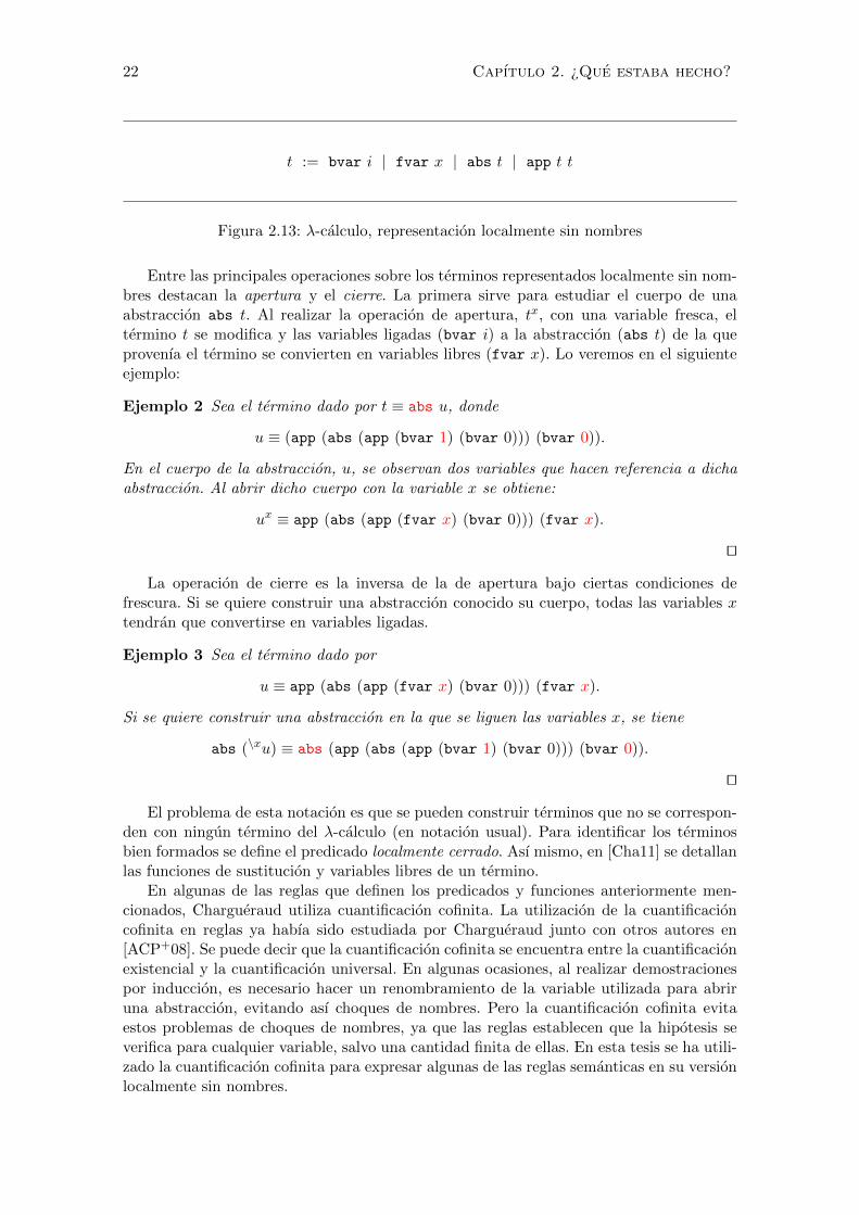
t := bvar i | fvar x | abs t | app t t
Figura 2.13: λ-calculo, representacion localmente sin nombres
Entre las principales operaciones sobre los terminos representados localmente sin nom-bres destacan la apertura y el cierre. La primera sirve para estudiar el cuerpo de unaabstraccion abs t. Al realizar la operacion de apertura, tx, con una variable fresca, eltermino t se modifica y las variables ligadas (bvar i) a la abstraccion (abs t) de la queprovenıa el termino se convierten en variables libres (fvar x). Lo veremos en el siguienteejemplo:
Ejemplo 2 Sea el termino dado por t ≡ abs u, donde
u ≡ (app (abs (app (bvar 1) (bvar 0))) (bvar 0)).
En el cuerpo de la abstraccion, u, se observan dos variables que hacen referencia a dichaabstraccion. Al abrir dicho cuerpo con la variable x se obtiene:
ux ≡ app (abs (app (fvar x) (bvar 0))) (fvar x).
ut
La operacion de cierre es la inversa de la de apertura bajo ciertas condiciones defrescura. Si se quiere construir una abstraccion conocido su cuerpo, todas las variables xtendran que convertirse en variables ligadas.
Ejemplo 3 Sea el termino dado por
u ≡ app (abs (app (fvar x) (bvar 0))) (fvar x).
Si se quiere construir una abstraccion en la que se liguen las variables x, se tiene
abs (\xu) ≡ abs (app (abs (app (bvar 1) (bvar 0))) (bvar 0)).
ut
El problema de esta notacion es que se pueden construir terminos que no se correspon-den con ningun termino del λ-calculo (en notacion usual). Para identificar los terminosbien formados se define el predicado localmente cerrado. Ası mismo, en [Cha11] se detallanlas funciones de sustitucion y variables libres de un termino.
En algunas de las reglas que definen los predicados y funciones anteriormente men-cionados, Chargueraud utiliza cuantificacion cofinita. La utilizacion de la cuantificacioncofinita en reglas ya habıa sido estudiada por Chargueraud junto con otros autores en[ACP+08]. Se puede decir que la cuantificacion cofinita se encuentra entre la cuantificacionexistencial y la cuantificacion universal. En algunas ocasiones, al realizar demostracionespor induccion, es necesario hacer un renombramiento de la variable utilizada para abriruna abstraccion, evitando ası choques de nombres. Pero la cuantificacion cofinita evitaestos problemas de choques de nombres, ya que las reglas establecen que la hipotesis severifica para cualquier variable, salvo una cantidad finita de ellas. En esta tesis se ha utili-zado la cuantificacion cofinita para expresar algunas de las reglas semanticas en su versionlocalmente sin nombres.
2.7. Asistentes de demostracion 23
2.7 Asistentes de demostracion
Durante los ultimos anos se han desarrollado distintas herramientas que permiten tra-bajar con demostraciones matematicas. Geuvers resume en [Geu09] la historia e ideas delos asistentes de demostracion (proof assistants). Hay que diferenciar entre estos y los lla-mados demostradores automaticos de teoremas (automated theorem provers). Mientras quelos segundos son sistemas dotados de una serie de procedimientos que permiten demostrarciertas formulas automaticamente, los primeros automatizan los aspectos principales en laconstruccion de demostraciones pero no son autonomos y necesitan “ser guiados” por unhumano en los pasos mas controvertidos de la demostracion. El usuario utilizara diferentestacticas que guiaran a la maquina para construir la demostracion. Aunque los demostra-dores automaticos han evolucionado mucho y ya son bastante utiles en la practica, parademostraciones demasiado complejas aun son insuficientes.
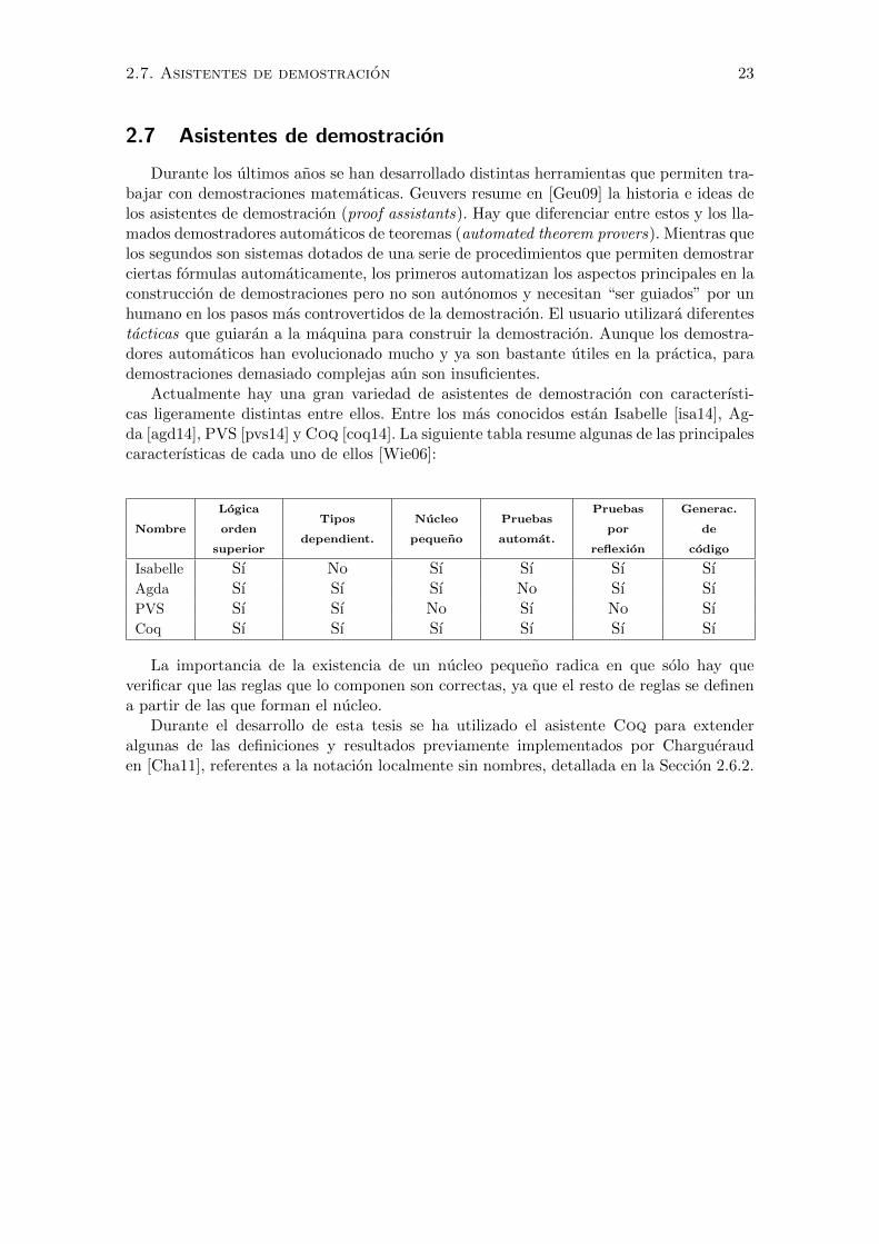
Actualmente hay una gran variedad de asistentes de demostracion con caracterısti-cas ligeramente distintas entre ellos. Entre los mas conocidos estan Isabelle [isa14], Ag-da [agd14], PVS [pvs14] y Coq [coq14]. La siguiente tabla resume algunas de las principalescaracterısticas de cada uno de ellos [Wie06]:
Nombre
Logica
orden
superior
Tipos
dependient.
Nucleo
pequeno
Pruebas
automat.
Pruebas
por
reflexion
Generac.
de
codigo
Isabelle Sı No Sı Sı Sı SıAgda Sı Sı Sı No Sı SıPVS Sı Sı No Sı No SıCoq Sı Sı Sı Sı Sı Sı
La importancia de la existencia de un nucleo pequeno radica en que solo hay queverificar que las reglas que lo componen son correctas, ya que el resto de reglas se definena partir de las que forman el nucleo.
Durante el desarrollo de esta tesis se ha utilizado el asistente Coq para extenderalgunas de las definiciones y resultados previamente implementados por Charguerauden [Cha11], referentes a la notacion localmente sin nombres, detallada en la Seccion 2.6.2.

24 Capıtulo 2. ¿Que estaba hecho?
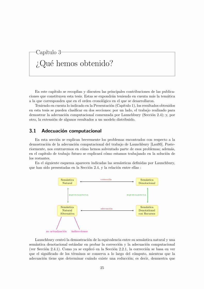
Capıtulo 3
¿Que hemos obtenido?
En este capıtulo se recopilan y discuten las principales contribuciones de las publica-ciones que constituyen esta tesis. Estas se expondran teniendo en cuenta mas la tematicaa la que corresponden que en el orden cronologico en el que se desarrollaron.
Teniendo en cuenta lo indicado en la Presentacion (Capıtulo 1), los resultados obtenidosen esta tesis se pueden clasificar en dos secciones: por un lado, el trabajo realizado parademostrar la adecuacion computacional comenzada por Launchbury (Seccion 2.4); y, porotro, la extension de algunos resultados a un modelo distribuido.
3.1 Adecuacion computacional
En esta seccion se explican brevemente los problemas encontrados con respecto a lademostracion de la adecuacion computacional del trabajo de Launchbury [Lau93]. Poste-riormente, nos centraremos en como hemos solventado parte de esos problemas; ademas,en el capıtulo de trabajo futuro se explicara como estamos trabajando en la solucion delos restantes.
En el siguiente esquema aparecen indicadas las semanticas definidas por Launchbury,que han sido presentadas en la Seccion 2.4, y la relacion entre ellas :
SemanticaNatural
SemanticaDenotacional
SemanticaNatural
Alternativa
SemanticaDenotationalcon Recursos
correccion
adecuacion
EQUIVALENCIA EQUIVALENCIA
no actualizacion indirecciones
Launchbury centro la demostracion de la equivalencia entre su semantica natural y unasemantica denotacional estandar en probar la correccion y la adecuacion computacional(ver Seccion 2.4.1). Como ya se explico en la Seccion 2.2.1, la correccion se basa en verque el significado de los terminos se conserva a lo largo del computo, mientras que laadecuacion tiene que determinar cuando existe una reduccion; es decir, demuestra que
25
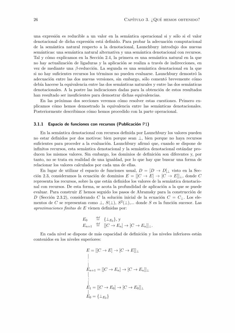
26 Capıtulo 3. ¿Que hemos obtenido?
una expresion es reducible a un valor en la semantica operacional si y solo si el valordenotacional de dicha expresion esta definido. Para probar la adecuacion computacionalde la semantica natural respecto a la denotacional, Launchbury introdujo dos nuevassemanticas: una semantica natural alternativa y una semantica denotacional con recursos.Tal y como explicamos en la Seccion 2.4, la primera es una semantica natural en la queno hay actualizacion de ligaduras y la aplicacion se realiza a traves de indirecciones, envez de mediante una β-reduccion. La segunda es una semantica denotacional en la quesi no hay suficientes recursos los terminos no pueden evaluarse. Launchbury demostro laadecuacion entre las dos nuevas versiones, sin embargo, solo comento brevemente comodebıa hacerse la equivalencia entre las dos semanticas naturales y entre las dos semanticasdenotacionales. A la postre las indicaciones dadas para la obtencion de estos resultadoshan resultado ser insuficientes para demostrar dichas equivalencias.
En las proximas dos secciones veremos como resolver estas cuestiones. Primero ex-plicamos como hemos demostrado la equivalencia entre las semanticas denotacionales.Posteriormente describimos como hemos procedido con la parte operacional.
3.1.1 Espacio de funciones con recursos (Publicacion P1)
En la semantica denotacional con recursos definida por Launchbury los valores puedenno estar definidos por dos motivos: bien porque sean ⊥, bien porque no haya recursossuficientes para proceder a la evaluacion. Launchbury afirmo que, cuando se dispone deinfinitos recursos, esta semantica denotacional y la semantica denotacional estandar pro-ducen los mismos valores. Sin embargo, los dominios de definicion son diferentes y, portanto, no se trata en realidad de una igualdad, por lo que hay que buscar una forma derelacionar los valores calculados por cada una de ellas.
En lugar de utilizar el espacio de funciones usual, D = [D → D]⊥ visto en la Sec-cion 2.3, consideramos la ecuacion de dominios E = [[C → E] → [C → E]]⊥, donde Crepresenta los recursos, sobre la que estan definidos los valores de la semantica denotacio-nal con recursos. De esta forma, se acota la profundidad de aplicacion a la que se puedeevaluar. Para construir E hemos seguido los pasos de Abramsky para la construccion deD (Seccion 2.3.2), considerando C la solucion inicial de la ecuacion C = C⊥. Los ele-mentos de C se representan como ⊥, S(⊥), S2(⊥),... donde S es la funcion sucesor. Lasaproximaciones finitas de E vienen definidas por:
E0def= {⊥E0}, y
En+1def= [[C → En]→ [C → En]]⊥.
En cada nivel se dispone de mas capacidad de definicion y los niveles inferiores estancontenidos en los niveles superiores:
E0 = {⊥E0}
|E1 = [[C → E0] → [C → E0]]⊥|
...|En+1 = [[C → En] → [C → En]]⊥|
..
.
|
E = [[C → E] → [C → E]]⊥
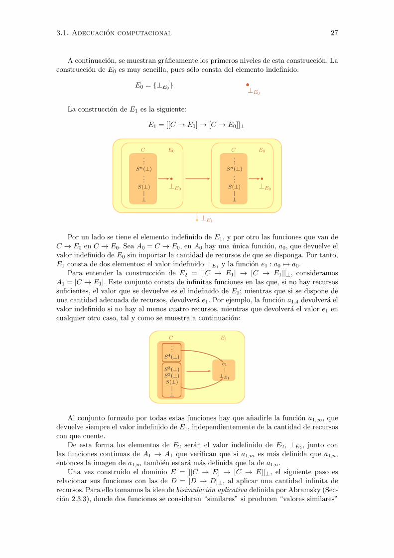
3.1. Adecuacion computacional 27
A continuacion, se muestran graficamente los primeros niveles de esta construccion. Laconstruccion de E0 es muy sencilla, pues solo consta del elemento indefinido:
E0 = {⊥E0}
⊥E0
La construccion de E1 es la siguiente:
E1 = [[C → E0] → [C → E0]]⊥
C E0
.
.
.Sn(⊥)
.
.
.S(⊥)
|⊥
b
C E0
.
.
.Sn(⊥)
.
.
.S(⊥)
|⊥
b
b ⊥E1
⊥E0⊥E0
Por un lado se tiene el elemento indefinido de E1, y por otro las funciones que van deC → E0 en C → E0. Sea A0 = C → E0, en A0 hay una unica funcion, a0, que devuelve elvalor indefinido de E0 sin importar la cantidad de recursos de que se disponga. Por tanto,E1 consta de dos elementos: el valor indefinido ⊥E1 y la funcion e1 : a0 7→ a0.
Para entender la construccion de E2 = [[C → E1] → [C → E1]]⊥, consideramosA1 = [C → E1]. Este conjunto consta de infinitas funciones en las que, si no hay recursossuficientes, el valor que se devuelve es el indefinido de E1; mientras que si se dispone deuna cantidad adecuada de recursos, devolvera e1. Por ejemplo, la funcion a1,4 devolvera elvalor indefinido si no hay al menos cuatro recursos, mientras que devolvera el valor e1 encualquier otro caso, tal y como se muestra a continuacion:
C E1
.
.
.S4(⊥)
S3(⊥)S2(⊥)S(⊥)
|⊥
e1
|⊥E1
Al conjunto formado por todas estas funciones hay que anadirle la funcion a1,∞, quedevuelve siempre el valor indefinido de E1, independientemente de la cantidad de recursoscon que cuente.
De esta forma los elementos de E2 seran el valor indefinido de E2, ⊥E2 , junto conlas funciones continuas de A1 → A1 que verifican que si a1,m es mas definida que a1,n,entonces la imagen de a1,m tambien estara mas definida que la de a1,n.
Una vez construido el dominio E = [[C → E] → [C → E]]⊥, el siguiente paso esrelacionar sus funciones con las de D = [D → D]⊥, al aplicar una cantidad infinita derecursos. Para ello tomamos la idea de bisimulacion aplicativa definida por Abramsky (Sec-cion 2.3.3), donde dos funciones se consideran “similares” si producen “valores similares”
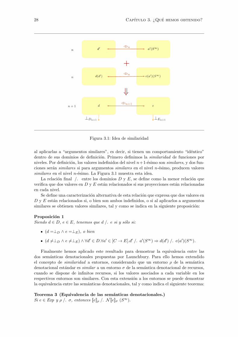
28 Capıtulo 3. ¿Que hemos obtenido?
d′ a′(S∞)n
⊳⊲n
+
d(d′) e(a′)(S∞)n
⊳⊲n
⇓
d en+ 1
⊥Dn+1⊥En+1
⊳⊲n+1
Figura 3.1: Idea de similaridad
al aplicarlas a “argumentos similares”, es decir, si tienen un comportamiento “identico”dentro de sus dominios de definicion. Primero definimos la similaridad de funciones porniveles. Por definicion, los valores indefinidos del nivel n+1-esimo son similares, y dos fun-ciones seran similares si para argumentos similares en el nivel n-esimo, producen valoressimilares en el nivel n-esimo. La Figura 3.1 muestra esta idea.
La relacion final /. entre los dominios D y E, se define como la menor relacion queverifica que dos valores en D y E estan relacionados si sus proyecciones estan relacionadasen cada nivel.
Se define una caracterizacion alternativa de esta relacion que expresa que dos valores enD y E estan relacionados si, o bien son ambos indefinidos, o si al aplicarlos a argumentossimilares se obtienen valores similares, tal y como se indica en la siguiente proposicion:
Proposicion 1Siendo d ∈ D, e ∈ E, tenemos que d /. e si y solo si:
(d =⊥D ∧ e =⊥E), o bien
(d 6=⊥D ∧ e 6=⊥E) ∧ ∀d′ ∈ D.∀a′ ∈ [C → E].d′ /. a′(S∞)⇒ d(d′) /. e(a′)(S∞).
Finalmente hemos aplicado este resultado para demostrar la equivalencia entre lasdos semanticas denotacionales propuestas por Launchbury. Para ello hemos extendidoel concepto de similaridad a entornos, considerando que un entorno ρ de la semanticadenotacional estandar es similar a un entorno σ de la semantica denotacional de recursos,cuando se dispone de infinitos recursos, si los valores asociados a cada variable en losrespectivos entornos son similares. Con esta extension a los entornos se puede demostrarla equivalencia entre las semanticas denotacionales, tal y como indica el siguiente teorema:
Teorema 3 (Equivalencia de las semanticas denotacionales.)Si e ∈ Exp y ρ /. σ, entonces [[e]]ρ /. N [[e]]σ (S∞).
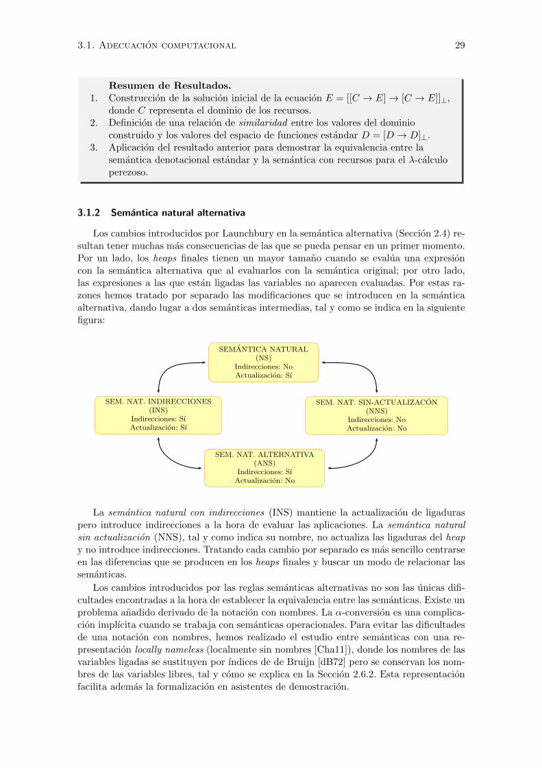
3.1. Adecuacion computacional 29
Resumen de Resultados.
1. Construccion de la solucion inicial de la ecuacion E = [[C → E] → [C → E]]⊥,donde C representa el dominio de los recursos.
2. Definicion de una relacion de similaridad entre los valores del dominioconstruido y los valores del espacio de funciones estandar D = [D → D]⊥.
3. Aplicacion del resultado anterior para demostrar la equivalencia entre lasemantica denotacional estandar y la semantica con recursos para el λ-calculoperezoso.
3.1.2 Semantica natural alternativa
Los cambios introducidos por Launchbury en la semantica alternativa (Seccion 2.4) re-sultan tener muchas mas consecuencias de las que se pueda pensar en un primer momento.Por un lado, los heaps finales tienen un mayor tamano cuando se evalua una expresioncon la semantica alternativa que al evaluarlos con la semantica original; por otro lado,las expresiones a las que estan ligadas las variables no aparecen evaluadas. Por estas ra-zones hemos tratado por separado las modificaciones que se introducen en la semanticaalternativa, dando lugar a dos semanticas intermedias, tal y como se indica en la siguientefigura:
SEMANTICA NATURAL(NS)
Indirecciones: NoActualizacion: Sı
SEM. NAT. INDIRECCIONES(INS)
Indirecciones: SıActualizacion: Sı
SEM. NAT. SIN-ACTUALIZACON(NNS)
Indirecciones: NoActualizacion: No
SEM. NAT. ALTERNATIVA(ANS)
Indirecciones: SıActualizacion: No
La semantica natural con indirecciones (INS) mantiene la actualizacion de ligaduraspero introduce indirecciones a la hora de evaluar las aplicaciones. La semantica naturalsin actualizacion (NNS), tal y como indica su nombre, no actualiza las ligaduras del heapy no introduce indirecciones. Tratando cada cambio por separado es mas sencillo centrarseen las diferencias que se producen en los heaps finales y buscar un modo de relacionar lassemanticas.
Los cambios introducidos por las reglas semanticas alternativas no son las unicas difi-cultades encontradas a la hora de establecer la equivalencia entre las semanticas. Existe unproblema anadido derivado de la notacion con nombres. La α-conversion es una complica-cion implıcita cuando se trabaja con semanticas operacionales. Para evitar las dificultadesde una notacion con nombres, hemos realizado el estudio entre semanticas con una re-presentacion locally nameless (localmente sin nombres [Cha11]), donde los nombres de lasvariables ligadas se sustituyen por ındices de de Bruijn [dB72] pero se conservan los nom-bres de las variables libres, tal y como se explica en la Seccion 2.6.2. Esta representacionfacilita ademas la formalizacion en asistentes de demostracion.

30 Capıtulo 3. ¿Que hemos obtenido?
x ∈ Id i, j ∈ Nv ∈ Var ::= bvar i j | fvar xt ∈ LNExp ::= v | abs t | app t v | let {ti}ni=1 in t
Figura 3.2: Sintaxis localmente sin nombres
Representacion localmente sin nombres (Publicacion P2 y TechRep TR1)
Se procede a explicar como hemos extendido con declaraciones locales recursivas larepresentacion localmente sin nombres del λ-calculo dada por Chargueraud en [Cha11].Al eliminar los nombres de las variables ligadas se evita tener que trabajar con clases deequivalencia y elegir un representante de ellas, pues todos los terminos cerrados que seansemanticamente iguales se representan de manera unica.
Como se ha visto en la Seccion 2.6.2, Chargueraud explica y desarrolla las ventajas dela representacion localmente sin nombres para un lenguaje con variables, abstracciones yaplicaciones. Como se observa en la Figura 2.4 de la Seccion 2.4, en el calculo utilizado porLaunchbury, ademas de las expresiones anteriores se consideran declaraciones locales re-cursivas. Tal y como indica Chargueraud, las variables ligadas en estos casos se representancon dos ındices: el primero indica a que constructor esta ligada —una abstraccion o unadeclaracion local— tal y como se explica en la Seccion 2.6.1 y puede verse en el Ejemplo 1;el segundo ındice indica, dentro del constructor que liga la variable, a que expresion nosreferimos (cuando el constructor es una declaracion local, indica a que variable local sehace la referencia). El resultado es la sintaxis que se muestra en la Figura 3.2, donde Varrepresenta un conjunto de variables que pueden ser ligadas (bvar i j) o libres (fvar x).
El siguiente ejemplo ilustra como se determinan los ındices de las variables ligadas.
Ejemplo 4 La expresion e es una λ-abstraccion cuya expresion interna es un let con dosdefiniciones locales.
e ≡ λz.let x1 = λy1.y1,x2 = λy2.y2,
in (z x2)
La representacion de esta expresion con la notacion localmente sin nombres viene dadapor el termino t:
t ≡ abs (let abs (bvar 0 0), abs (bvar 0 0) in app (bvar 1 0) (bvar 0 1)).
En verde aparece la expresion ligada a x1, en rojo la de x2 y en azul el termino principal.
Si nos fijamos en el arbol sintactico veremos como los primeros ındices senalan a losconstructores que ligan:
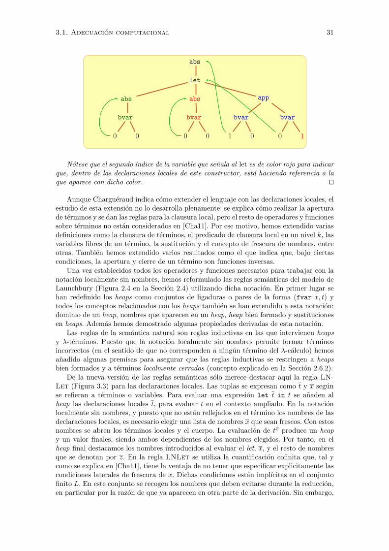
3.1. Adecuacion computacional 31
abs
let
abs abs app
bvar bvar bvar bvar
0 0 0 0 1 0 0 1
Notese que el segundo ındice de la variable que senala al let es de color rojo para indicarque, dentro de las declaraciones locales de este constructor, esta haciendo referencia a laque aparece con dicho color. ut
Aunque Chargueraud indica como extender el lenguaje con las declaraciones locales, elestudio de esta extension no lo desarrolla plenamente: se explica como realizar la aperturade terminos y se dan las reglas para la clausura local, pero el resto de operadores y funcionessobre terminos no estan considerados en [Cha11]. Por ese motivo, hemos extendido variasdefiniciones como la clausura de terminos, el predicado de clausura local en un nivel k, lasvariables libres de un termino, la sustitucion y el concepto de frescura de nombres, entreotras. Tambien hemos extendido varios resultados como el que indica que, bajo ciertascondiciones, la apertura y cierre de un termino son funciones inversas.
Una vez establecidos todos los operadores y funciones necesarios para trabajar con lanotacion localmente sin nombres, hemos reformulado las reglas semanticas del modelo deLaunchbury (Figura 2.4 en la Seccion 2.4) utilizando dicha notacion. En primer lugar sehan redefinido los heaps como conjuntos de ligaduras o pares de la forma (fvar x, t) ytodos los conceptos relacionados con los heaps tambien se han extendido a esta notacion:dominio de un heap, nombres que aparecen en un heap, heap bien formado y sustitucionesen heaps. Ademas hemos demostrado algunas propiedades derivadas de esta notacion.
Las reglas de la semantica natural son reglas inductivas en las que intervienen heapsy λ-terminos. Puesto que la notacion localmente sin nombres permite formar terminosincorrectos (en el sentido de que no corresponden a ningun termino del λ-calculo) hemosanadido algunas premisas para asegurar que las reglas inductivas se restringen a heapsbien formados y a terminos localmente cerrados (concepto explicado en la Seccion 2.6.2).
De la nueva version de las reglas semanticas solo merece destacar aquı la regla LN-Let (Figura 3.3) para las declaraciones locales. Las tuplas se expresan como t y x segunse refieran a terminos o variables. Para evaluar una expresion let t in t se anaden alheap las declaraciones locales t, para evaluar t en el contexto ampliado. En la notacionlocalmente sin nombres, y puesto que no estan reflejados en el termino los nombres de lasdeclaraciones locales, es necesario elegir una lista de nombres x que sean frescos. Con estosnombres se abren los terminos locales y el cuerpo. La evaluacion de tx produce un heapy un valor finales, siendo ambos dependientes de los nombres elegidos. Por tanto, en elheap final destacamos los nombres introducidos al evaluar el let, x, y el resto de nombresque se denotan por z. En la regla LNLet se utiliza la cuantificacion cofinita que, tal ycomo se explica en [Cha11], tiene la ventaja de no tener que especificar explicitamente lascondiciones laterales de frescura de x. Dichas condiciones estan implıcitas en el conjuntofinito L. En este conjunto se recogen los nombres que deben evitarse durante la reduccion,en particular por la razon de que ya aparecen en otra parte de la derivacion. Sin embargo,
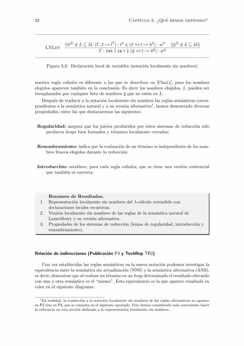
32 Capıtulo 3. ¿Que hemos obtenido?
LNLet∀x|t| /∈ L ⊆ Id (Γ, x 7→ t
x) : tx ⇓ (x++z 7→ ux) : wx {y|t| /∈ L ⊆ Id}
Γ : let t in t ⇓ (y ++z 7→ uy) : wy
Figura 3.3: Declaracion local de variables (notacion localmente sin nombres)
nuestra regla cofinita es diferente a las que se describen en [Cha11], pues los nombreselegidos aparecen tambien en la conclusion. Es decir los nombres elegidos, x, pueden serreemplazados por cualquier lista de nombres y que no esten en L.
Despues de traducir a la notacion localmente sin nombres las reglas semanticas corres-pondientes a la semantica natural y a su version alternativa1, hemos demostrado diversaspropiedades, entre las que destacaremos las siguientes:
Regularidad: asegura que los juicios producidos por estos sistemas de reduccion soloproducen heaps bien formados y terminos localmente cerrados;
Renombramiento: indica que la evaluacion de un termino es independiente de los nom-bres frescos elegidos durante la reduccion;
Introduccion: establece, para cada regla cofinita, que se tiene una version existencialque tambien es correcta.
Resumen de Resultados.
1. Representacion localmente sin nombres del λ-calculo extendido condeclaraciones locales recursivas.
2. Version localmente sin nombres de las reglas de la semantica natural deLaunchbury y su version alternativa.
3. Propiedades de los sistemas de reduccion (lemas de regularidad, introduccion yrenombramiento).
Relacion de indirecciones (Publicacion P3 y TechRep TR2)
Una vez establecidas las reglas semanticas en la nueva notacion podemos investigar laequivalencia entre la semantica sin actualizacion (NNS) y la semantica alternativa (ANS),es decir, demostrar que al evaluar un termino en un heap determinado el resultado obtenidocon una y otra semantica es el “mismo”. Esta equivalencia es la que aparece resaltada encolor en el siguiente diagrama:
1En realidad, la traduccion a la notacion localmente sin nombres de las reglas alternativas no apareceen P2 sino en P3, que se comenta en el siguiente apartado. Pero hemos considerado mas conveniente hacerla referencia en esta seccion dedicada a la representacion localmente sin nombres.

3.1. Adecuacion computacional 33
SEMANTICA NATURAL(NS)
Indirecciones: NoActualizacion: Sı
SEM. NAT. INDIRECCIONES(INS)
Indirecciones: SıActualizacion: Sı
SEM. NAT. SIN-ACTUALIZACION(NNS)
Indirecciones: NoActualizacion: No
SEM. NAT. ALTERNATIVA(ANS)
Indirecciones: SıActualizacion: No
Las semanticas NNS y ANS utilizan las mismas reglas de derivacion excepto por laregla de aplicacion, que en el caso de NNS aplica la regla LNApp, donde la aplicacionse realiza mediante una β-reduccion, y en el caso de ANS aplica la regla ALNApp, enla que se introduce una indireccion en el heap. Aunque esta diferencia parece inocua, loprimero que se observa es que los heaps finales obtenidos tras aplicar las reglas de ANSpueden ser mas grandes que los obtenidos tras aplicar las reglas de NNS, ya que cada vezque se evalua una aplicacion, se introduce una ligadura “extra” en el heap. Esta ligaduraes una indireccion, es decir, una variable ligada a otra variable. Por ello los heaps finalesobtenidos no pueden ser exactamente los mismos y hay que estudiar que relacion existeentre ellos. Teniendo en cuenta este dato, lo primero en lo que se penso fue en eliminarlas indirecciones y comprobar si los heaps finales obtenidos eran iguales. Sin embargo,esto no es suficiente, ya que en el heap final puede haber terminos que dependan de lasindirecciones que se han eliminado.
En el siguiente ejemplo se muestra este problema, donde ⇓N representa la evaluacioncon NNS y ⇓A la evaluacion con ANS:
Ejemplo 5 Considerense los siguientes terminos:
t ≡ let abs (bvar 0 0) in app (abs s) (bvar 0 0)s ≡ let abs (bvar 0 0), app (bvar 0 0) (bvar 1 0) in abs (bvar 0 0)
Al evaluar t en el contexto de un heap vacıo con las dos semanticas en estudio, se obtieneen ambos casos abs (bvar 0 0) como valor final y los siguientes heaps, respectivamente:
{ } : t
⇓N
x0 7→ abs (bvar 0 0),x1 7→ abs (bvar 0 0),x2 7→ app (fvar x1) (fvar x0)
{ } : t
⇓A
x0 7→ abs (bvar 0 0),x1 7→ abs (bvar 0 0),x2 7→ app (fvar x1) (fvar y)y 7→ (fvar x0)
Se observa que el heap obtenido al evaluar el termino con la semantica alternativa contieneuna ligadura mas, y que el termino asociado a la variable x2 depende de dicha ligaduraextra. ut
Por tanto, la relacion que buscamos entre heaps no puede consistir solo en eliminar lasindirecciones, sino que tambien es necesario realizar una sustitucion para cambiar todas
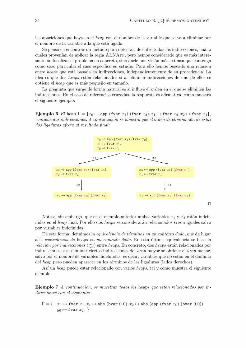
34 Capıtulo 3. ¿Que hemos obtenido?
las apariciones que haya en el heap con el nombre de la variable que se va a eliminar porel nombre de la variable a la que esta ligada.
Se penso en encontrar un metodo para detectar, de entre todas las indirecciones, cual ocuales provenıan de aplicar la regla ALNApp, pero hemos considerado que es mas intere-sante no focalizar el problema en concreto, sino darle una vision mas extensa que contengacomo caso particular el caso especıfico en estudio. Para ello hemos buscado una relacionentre heaps que este basada en indirecciones, independientemente de su procedencia. Laidea es que dos heaps esten relacionados si al eliminar indirecciones de uno de ellos seobtiene el heap que es mas pequeno en tamano.
La pregunta que surge de forma natural es si influye el orden en el que se eliminen lasindirecciones. En el caso de referencias cruzadas, la respuesta es afirmativa, como muestrael siguiente ejemplo:
Ejemplo 6 El heap Γ = {x0 7→ app (fvar x1) (fvar x2), x1 7→ fvar x2, x2 7→ fvar x1},contiene dos indirecciones. A continuacion se muestra que el orden de eliminacion de estasdos ligaduras afecta al resultado final:
x0 7→ app (fvar x1) (fvar x2),x1 7→ fvar x2,
x2 7→ fvar x1
x0 7→ app (fvar x2) (fvar x2),x2 7→ fvar x2
x0 7→ app (fvar x1) (fvar x1),x1 7→ fvar x1
x0 7→ app (fvar x2) (fvar x2) x0 7→ app (fvar x1) (fvar x1)
x1 x2
x2 x1
ut
Notese, sin embargo, que en el ejemplo anterior ambas variables x1 y x2 estan indefi-nidas en el heap final. Por ello dos heaps se consideraran relacionados si son iguales salvopor variables indefinidas.
De esta forma, definimos la equivalencia de terminos en un contexto dado, que da lugara la equivalencia de heaps en un contexto dado. En esta ultima equivalencia se basa larelacion por indirecciones (%I) entre heaps. En concreto, dos heaps estan relacionados porindirecciones si al eliminar ciertas indirecciones del heap mayor se obtiene el heap menor,salvo por el nombre de variables indefinidas, es decir, variables que no estan en el dominiodel heap pero pueden aparecer en los terminos de las ligaduras (lados derechos).
Ası un heap puede estar relacionado con varios heaps, tal y como muestra el siguienteejemplo.
Ejemplo 7 A continuacion, se muestran todos los heaps que estan relacionados por in-direcciones con el siguiente:
Γ = { x0 7→ fvar x1, x1 7→ abs (bvar 0 0), x2 7→ abs (app (fvar x0) (bvar 0 0)),y0 7→ fvar x2 }

3.1. Adecuacion computacional 35
x0 7→ fvar x1,
x1 7→ abs (bvar 0 0),x2 7→ abs (app (fvar x0) (bvar 0 0)),y0 7→ fvar x2
x0 7→ fvar x1,
x1 7→ abs (bvar 0 0),x2 7→ abs (app (fvar x0) (bvar 0 0)),y0 7→ fvar x2
x0 7→ fvar x1,
x1 7→ abs (bvar 0 0),x2 7→ abs (app (fvar x0) (bvar 0 0))
x1 7→ abs (bvar 0 0),x2 7→ abs (app (fvar x1) (bvar 0 0)),y0 7→ fvar x2
x1 7→ abs (bvar 0 0),x2 7→ abs (app (fvar x1) (bvar 0 0))
[ ]
[y0]
[x0]
[x0, y0]
ut
Extendemos esta relacion a pares (heap, termino) y enunciamos y demostramos elteorema que establece que si un termino evalua en un contexto dado con NNS, tambien lohace con ANS, y viceversa; y ademas, los pares (heap, termino) finales estan relacionadospor indirecciones.
Teorema 4 (Equivalencia ANS y NNS.)
eq an Γ : t ⇓A ∆A : wA ⇒∃∆N ∈ LNHeap . ∃wN ∈ LNVal .Γ : t ⇓N ∆N : wN ∧ (∆A : wA) %I (∆N : wN )
eq na Γ : t ⇓N ∆N : wN ⇒∃∆A ∈ LNHeap .∃wA ∈ LNVal . ∃x ⊆ dom(∆N )− dom(Γ) .∃y ⊆ Id . |x| = |y| ∧Γ : t ⇓A ∆A : wA ∧ (∆A : wA) %I (∆N [y/x] : wN [y/x])
En la segunda parte del teorema, eq na, se indica que es posible que haga falta unrenombramiento, pero este afectara solo a los nombres que han sido anadidos durante laevaluacion. Con NNS, algunos de los nombres del termino a evaluar pueden desaparecerdurante la evaluacion y ser introducidos de nuevo como “frescos”; sin embargo, al evaluarcon ANS esto no puede ocurrir, tal y como muestra el siguiente ejemplo:
Ejemplo 8 Considerese el termino
t ≡ let abs (bvar 1 1), let abs (bvar 0 0) in (bvar 0 0) in app (bvar 0 0) (fvar z)
Al evaluarlo en un contexto vacıo con NNS, la variable z desaparece del termino (y delheap); por el contrario, al evaluarlo con ANS se introduce en el heap mediante una indi-reccion. A continuacion, se muestra la derivacion de la evaluacion del termino con NNS:

36 Capıtulo 3. ¿Que hemos obtenido?
{ } : t{x0 7→ abs (fvar x1), x1 7→ let abs (bvar 0 0) in (bvar 0 0)} : app (fvar x0) (fvar z)
{x0 7→ abs (fvar x1), x1 7→ let abs (bvar 0 0) in (bvar 0 0)} : fvar x0{x0 7→ abs (fvar x1), x1 7→ let abs (bvar 0 0) in (bvar 0 0)} : abs fvar x1{x0 7→ abs (fvar x1), x1 7→ let abs (bvar 0 0) in (bvar 0 0)} : abs fvar x1
{x0 7→ abs (fvar x1), x1 7→ let abs (bvar 0 0) in (bvar 0 0)} : abs fvar x1
{x0 7→ abs (fvar x1), x1 7→ let abs (bvar 0 0) in (bvar 0 0)} : fvar x1{x0 7→ abs (fvar x1), x1 7→ let abs (bvar 0 0) in (bvar 0 0)} : let abs (bvar 0 0) in (bvar 0 0)...{x0 7→ abs (fvar x1), x1 7→ let abs (bvar 0 0) in (bvar 0 0),x2 7→ abs (bvar 0 0)
}: abs (bvar 0 0)
{x0 7→ abs (fvar x1), x1 7→ let abs (bvar 0 0) in (bvar 0 0),x2 7→ abs (bvar 0 0)
}: abs (bvar 0 0)
{x0 7→ abs (fvar x1), x1 7→ let abs (bvar 0 0) in (bvar 0 0), x2 7→ abs (bvar 0 0)} : abs (bvar 0 0){x0 7→ abs (fvar x1), x1 7→ let abs (bvar 0 0) in (bvar 0 0), x2 7→ abs (bvar 0 0)} : abs (bvar 0 0)
Al realizar la β-reduccion, el nombre z ya no aparece mas, por lo que al introducir lavariable fresca x2 en el heap, se podrıa haber elegido como nombre z.
Sin embargo, al realizar la evaluacion con la semantica alternativa, se introduce z enel heap mediante una indireccion, y ya no puede ser elegido cuando se necesite un nombre“fresco”.
{ } : t{x0 7→ abs (fvar x1), x1 7→ let abs (bvar 0 0) in (bvar 0 0)} : app (fvar x0) (fvar z)
{x0 7→ abs (fvar x1), x1 7→ let abs (bvar 0 0) in (bvar 0 0)} : fvar x0{x0 7→ abs (fvar x1), x1 7→ let abs (bvar 0 0) in (bvar 0 0)} : abs fvar x1{x0 7→ abs (fvar x1), x1 7→ let abs (bvar 0 0) in (bvar 0 0)} : abs fvar x1
{x0 7→ abs (fvar x1), x1 7→ let abs (bvar 0 0) in (bvar 0 0)} : abs fvar x1
{x0 7→ abs (fvar x1), x1 7→ let abs (bvar 0 0) in (bvar 0 0), y 7→ fvar z} : fvar x1{x0 7→ abs (fvar x1), y 7→ fvar z,x1 7→ let abs (bvar 0 0) in (bvar 0 0)
}: let abs (bvar 0 0) in (bvar 0 0)
...{x0 7→ abs (fvar x1), x1 7→ let abs (bvar 0 0) in (bvar 0 0),y 7→ fvar z, x2 7→ abs (bvar 0 0)
}: abs (bvar 0 0)
{x0 7→ abs (fvar x1), x1 7→ let abs (bvar 0 0) in (bvar 0 0),y 7→ fvar z, x2 7→ abs (bvar 0 0)
}: abs (bvar 0 0)
{x0 7→ abs (fvar x1), x1 7→ let abs (bvar 0 0) in (bvar 0 0),y 7→ fvar z, x2 7→ abs (bvar 0 0)
}: abs (bvar 0 0)
{x0 7→ abs (fvar x1), x1 7→ let abs (bvar 0 0) in (bvar 0 0),y 7→ fvar z, x2 7→ abs (bvar 0 0)
}: abs (bvar 0 0)
ut
La demostracion del teorema no puede realizarse directamente mediante una induc-cion por reglas, pues en las subderivaciones el heap y los terminos de los que se parteno son iguales, sino que estan relacionados por indirecciones. Por esta razon, es necesariala demostracion de un resultado mas general, en el que se establece la relacion entre lasderivaciones de las dos semanticas en estudio partiendo de pares (heap, termino) relaciona-dos por indirecciones (Proposicion 2). Puesto que en las derivaciones se van introduciendovariables frescas en el heap, siempre que haya una derivacion habra de hecho infinitas,que se diferencian en los nombres frescos elegidos. La proposicion indica que partiendo
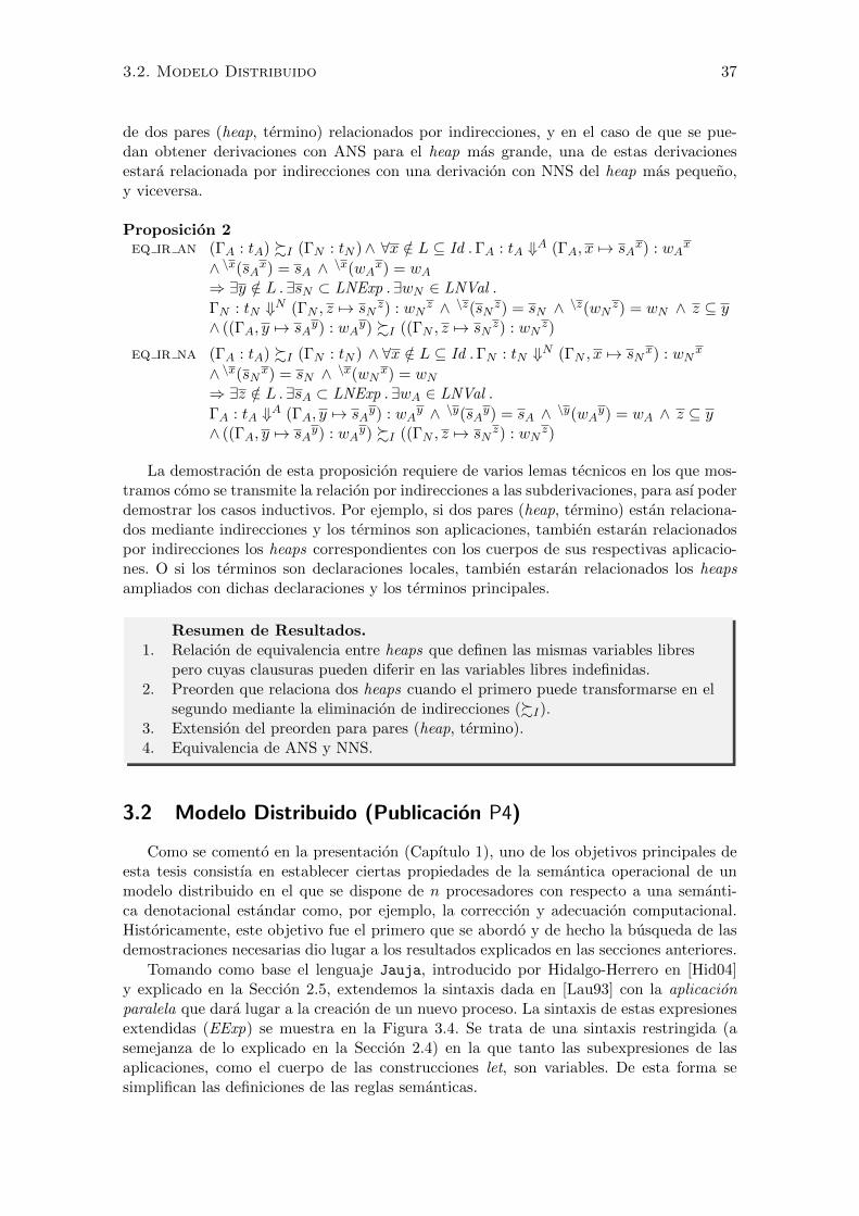
3.2. Modelo Distribuido 37
de dos pares (heap, termino) relacionados por indirecciones, y en el caso de que se pue-dan obtener derivaciones con ANS para el heap mas grande, una de estas derivacionesestara relacionada por indirecciones con una derivacion con NNS del heap mas pequeno,y viceversa.
Proposicion 2eq ir an (ΓA : tA) %I (ΓN : tN )∧ ∀x /∈ L ⊆ Id .ΓA : tA ⇓A (ΓA, x 7→ sA
x) : wAx
∧ \x(sAx) = sA ∧ \x(wA
x) = wA⇒ ∃y /∈ L .∃sN ⊂ LNExp .∃wN ∈ LNVal .
ΓN : tN ⇓N (ΓN , z 7→ sNz) : wN
z ∧ \z(sNz) = sN ∧ \z(wNz) = wN ∧ z ⊆ y∧ ((ΓA, y 7→ sA
y) : wAy) %I ((ΓN , z 7→ sN
z) : wNz)
eq ir na (ΓA : tA) %I (ΓN : tN ) ∧ ∀x /∈ L ⊆ Id .ΓN : tN ⇓N (ΓN , x 7→ sNx) : wN
x
∧ \x(sNx) = sN ∧ \x(wN
x) = wN⇒ ∃z /∈ L .∃sA ⊂ LNExp . ∃wA ∈ LNVal .
ΓA : tA ⇓A (ΓA, y 7→ sAy) : wA
y ∧ \y(sAy) = sA ∧ \y(wAy) = wA ∧ z ⊆ y∧ ((ΓA, y 7→ sA
y) : wAy) %I ((ΓN , z 7→ sN
z) : wNz)
La demostracion de esta proposicion requiere de varios lemas tecnicos en los que mos-tramos como se transmite la relacion por indirecciones a las subderivaciones, para ası poderdemostrar los casos inductivos. Por ejemplo, si dos pares (heap, termino) estan relaciona-dos mediante indirecciones y los terminos son aplicaciones, tambien estaran relacionadospor indirecciones los heaps correspondientes con los cuerpos de sus respectivas aplicacio-nes. O si los terminos son declaraciones locales, tambien estaran relacionados los heapsampliados con dichas declaraciones y los terminos principales.
Resumen de Resultados.
1. Relacion de equivalencia entre heaps que definen las mismas variables librespero cuyas clausuras pueden diferir en las variables libres indefinidas.
2. Preorden que relaciona dos heaps cuando el primero puede transformarse en elsegundo mediante la eliminacion de indirecciones (%I).
3. Extension del preorden para pares (heap, termino).4. Equivalencia de ANS y NNS.
3.2 Modelo Distribuido (Publicacion P4)
Como se comento en la presentacion (Capıtulo 1), uno de los objetivos principales deesta tesis consistıa en establecer ciertas propiedades de la semantica operacional de unmodelo distribuido en el que se dispone de n procesadores con respecto a una semanti-ca denotacional estandar como, por ejemplo, la correccion y adecuacion computacional.Historicamente, este objetivo fue el primero que se abordo y de hecho la busqueda de lasdemostraciones necesarias dio lugar a los resultados explicados en las secciones anteriores.
Tomando como base el lenguaje Jauja, introducido por Hidalgo-Herrero en [Hid04]y explicado en la Seccion 2.5, extendemos la sintaxis dada en [Lau93] con la aplicacionparalela que dara lugar a la creacion de un nuevo proceso. La sintaxis de estas expresionesextendidas (EExp) se muestra en la Figura 3.4. Se trata de una sintaxis restringida (asemejanza de lo explicado en la Seccion 2.4) en la que tanto las subexpresiones de lasaplicaciones, como el cuerpo de las construcciones let, son variables. De esta forma sesimplifican las definiciones de las reglas semanticas.
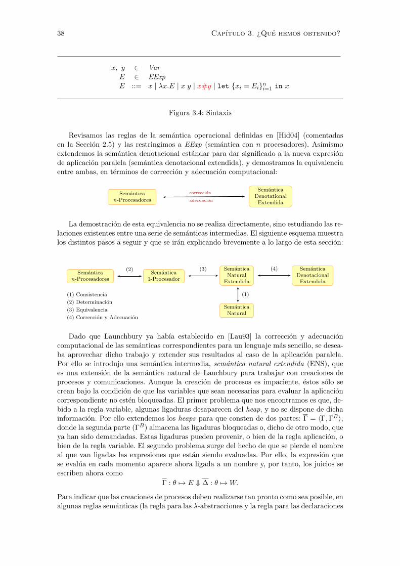
38 Capıtulo 3. ¿Que hemos obtenido?
x, y ∈ VarE ∈ EExpE ::= x | λx.E | x y | x#y | let {xi = Ei}ni=1 in x
Figura 3.4: Sintaxis
Revisamos las reglas de la semantica operacional definidas en [Hid04] (comentadasen la Seccion 2.5) y las restringimos a EExp (semantica con n procesadores). Asımismoextendemos la semantica denotacional estandar para dar significado a la nueva expresionde aplicacion paralela (semantica denotacional extendida), y demostramos la equivalenciaentre ambas, en terminos de correccion y adecuacion computacional:
Semantican-Procesadores
SemanticaDenotationalExtendida
correccion
adecuacion
La demostracion de esta equivalencia no se realiza directamente, sino estudiando las re-laciones existentes entre una serie de semanticas intermedias. El siguiente esquema muestralos distintos pasos a seguir y que se iran explicando brevemente a lo largo de esta seccion:
Semantican-Procesadores
Semantica1-Procesador
SemanticaNatural
Extendida
SemanticaNatural
SemanticaDenotacionalExtendida
(2) (3)
(1)
(4)
(1) Consistencia
(2) Determinacion
(3) Equivalencia
(4) Correccion y Adecuacion
Dado que Launchbury ya habıa establecido en [Lau93] la correccion y adecuacioncomputacional de las semanticas correspondientes para un lenguaje mas sencillo, se desea-ba aprovechar dicho trabajo y extender sus resultados al caso de la aplicacion paralela.Por ello se introdujo una semantica intermedia, semantica natural extendida (ENS), quees una extension de la semantica natural de Lauchbury para trabajar con creaciones deprocesos y comunicaciones. Aunque la creacion de procesos es impaciente, estos solo secrean bajo la condicion de que las variables que sean necesarias para evaluar la aplicacioncorrespondiente no esten bloqueadas. El primer problema que nos encontramos es que, de-bido a la regla variable, algunas ligaduras desaparecen del heap, y no se dispone de dichainformacion. Por ello extendemos los heaps para que consten de dos partes: Γ = 〈Γ,ΓB〉,donde la segunda parte (ΓB) almacena las ligaduras bloqueadas o, dicho de otro modo, queya han sido demandadas. Estas ligaduras pueden provenir, o bien de la regla aplicacion, obien de la regla variable. El segundo problema surge del hecho de que se pierde el nombreal que van ligadas las expresiones que estan siendo evaluadas. Por ello, la expresion quese evalua en cada momento aparece ahora ligada a un nombre y, por tanto, los juicios seescriben ahora como
Γ : θ 7→ E ⇓ ∆ : θ 7→W.
Para indicar que las creaciones de procesos deben realizarse tan pronto como sea posible, enalgunas reglas semanticas (la regla para las λ-abstracciones y la regla para las declaraciones
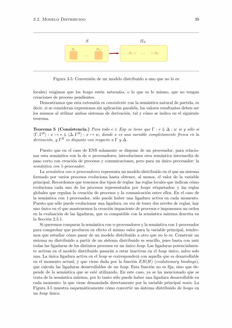
3.2. Modelo Distribuido 39
S
H1 Hn
.
.
.. . .
.
.
.
HS
H1 ∪ . . . ∪ Hn
Figura 3.5: Conversion de un modelo distribuido a uno que no lo es
locales) exigimos que los heaps esten saturados, o lo que es lo mismo, que no tengancreaciones de proceso pendientes.
Demostramos que esta extension es consistente con la semantica natural de partida, esdecir, si se consideran expresiones sin aplicacion paralela, los valores resultantes deben serlos mismos al utilizar ambos sistemas de derivacion, tal y como se indica en el siguienteteorema.
Teorema 5 (Consistencia.) Para todo e ∈ Exp se tiene que Γ : e ⇓ ∆ : w si y solo si〈Γ,ΓB〉 : x 7→ e ⇓ 〈∆,ΓB〉 : x 7→ w, donde x es una variable completamente fresca en laderivacion, y ΓB es disjunto con respecto a Γ y ∆.
Puesto que en el caso de ENS solamente se dispone de un procesador, para relacio-nar esta semantica con la de n procesadores, introducimos otra semantica intermedia depaso corto con creacion de procesos y comunicaciones, pero para un unico procesador: lasemantica con 1-procesador.
La semantica con n-procesadores representa un modelo distribuido en el que un sistemaformado por varios procesos evoluciona hasta obtener, al menos, el valor de la variableprincipal. Recordemos que tenemos dos tipos de reglas: las reglas locales que indican comoevoluciona cada uno de los procesos representados por heaps etiquetados; y las reglasglobales que regulan la creacion de procesos y la comunicacion entre ellos. En el caso dela semantica con 1-procesador, solo puede haber una ligadura activa en cada momento.Puesto que solo puede evolucionar una ligadura, en vez de tener dos niveles de reglas, hayuno unico en el que mantenemos la creacion impaciente de procesos e imponemos un ordenen la evaluacion de las ligaduras, que es compatible con la semantica mınima descrita enla Seccion 2.5.1.
Si queremos comparar la semantica con n-procesadores y la semantica con 1-procesadorpara comprobar que producen en efecto el mismo valor para la variable principal, tendre-mos que estudiar como pasar de un modelo distribuido a otro que no lo es. Construir unsistema no distribuido a partir de un sistema distribuido es sencillo, pues basta con unirtodas las ligaduras de los distintos procesos en un unico heap. Las ligaduras potencialmen-te activas en el modelo distribuido pasaran a estar inactivas en el heap unico, salvo solouna. La unica ligadura activa en el heap se correspondera con aquella que es desarrollableen el momento actual, y que viene dada por la funcion EB(H) (evolutionary bindings),que calcula las ligaduras desarrollables de un heap. Esta funcion no es fija, sino que de-pende de la semantica que se este utilizando. En este caso, ya se ha mencionado que setrata de la semantica mınima, por lo tanto solo puede haber una ligadura desarrollable encada momento: la que viene demandada directamente por la variable principal main. LaFigura 3.5 muestra esquematicamente como convertir un sistema distribuido de heaps enun heap unico.
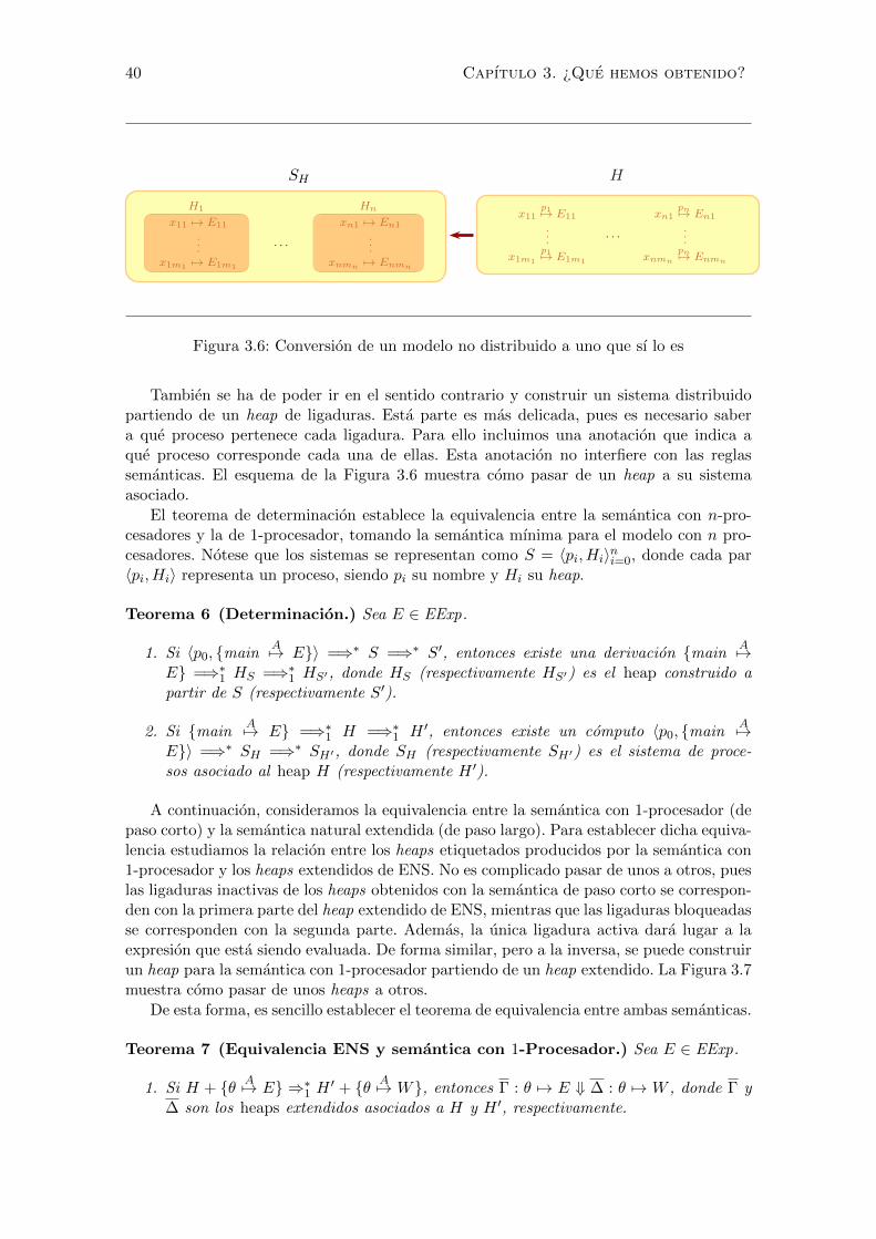
40 Capıtulo 3. ¿Que hemos obtenido?
SH
H1 Hn
x11 7→ E11
.
.
.x1m1
7→ E1m1
. . .
xn1 7→ En1
.
.
.xnmn
7→ Enmn
H
x11p17→ E11
.
.
.
x1m1
p17→ E1m1
. . .
xn1pn7→ En1
.
.
.
xnmn
pn7→ Enmn
Figura 3.6: Conversion de un modelo no distribuido a uno que sı lo es
Tambien se ha de poder ir en el sentido contrario y construir un sistema distribuidopartiendo de un heap de ligaduras. Esta parte es mas delicada, pues es necesario sabera que proceso pertenece cada ligadura. Para ello incluimos una anotacion que indica aque proceso corresponde cada una de ellas. Esta anotacion no interfiere con las reglassemanticas. El esquema de la Figura 3.6 muestra como pasar de un heap a su sistemaasociado.
El teorema de determinacion establece la equivalencia entre la semantica con n-pro-cesadores y la de 1-procesador, tomando la semantica mınima para el modelo con n pro-cesadores. Notese que los sistemas se representan como S = 〈pi, Hi〉ni=0, donde cada par〈pi, Hi〉 representa un proceso, siendo pi su nombre y Hi su heap.
Teorema 6 (Determinacion.) Sea E ∈ EExp.
1. Si 〈p0, {mainA7→ E}〉 =⇒∗ S =⇒∗ S′, entonces existe una derivacion {main
A7→E} =⇒∗1 HS =⇒∗1 HS′, donde HS (respectivamente HS′) es el heap construido apartir de S (respectivamente S′).
2. Si {mainA7→ E} =⇒∗1 H =⇒∗1 H ′, entonces existe un computo 〈p0, {main
A7→E}〉 =⇒∗ SH =⇒∗ SH′, donde SH (respectivamente SH′) es el sistema de proce-sos asociado al heap H (respectivamente H ′).
A continuacion, consideramos la equivalencia entre la semantica con 1-procesador (depaso corto) y la semantica natural extendida (de paso largo). Para establecer dicha equiva-lencia estudiamos la relacion entre los heaps etiquetados producidos por la semantica con1-procesador y los heaps extendidos de ENS. No es complicado pasar de unos a otros, pueslas ligaduras inactivas de los heaps obtenidos con la semantica de paso corto se correspon-den con la primera parte del heap extendido de ENS, mientras que las ligaduras bloqueadasse corresponden con la segunda parte. Ademas, la unica ligadura activa dara lugar a laexpresion que esta siendo evaluada. De forma similar, pero a la inversa, se puede construirun heap para la semantica con 1-procesador partiendo de un heap extendido. La Figura 3.7muestra como pasar de unos heaps a otros.
De esta forma, es sencillo establecer el teorema de equivalencia entre ambas semanticas.
Teorema 7 (Equivalencia ENS y semantica con 1-Procesador.) Sea E ∈ EExp.
1. Si H + {θ A7→ E} ⇒∗1 H ′ + {θA7→ W}, entonces Γ : θ 7→ E ⇓ ∆ : θ 7→ W , donde Γ y
∆ son los heaps extendidos asociados a H y H ′, respectivamente.
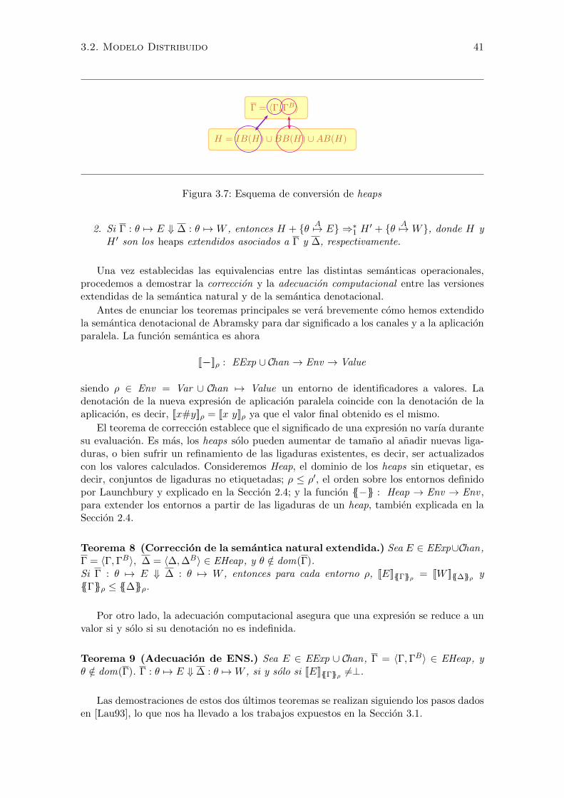
3.2. Modelo Distribuido 41
Γ = 〈Γ,ΓB〉
H = IB(H) ∪BB(H) ∪AB(H)
Figura 3.7: Esquema de conversion de heaps
2. Si Γ : θ 7→ E ⇓ ∆ : θ 7→ W , entonces H + {θ A7→ E} ⇒∗1 H ′ + {θA7→ W}, donde H y
H ′ son los heaps extendidos asociados a Γ y ∆, respectivamente.
Una vez establecidas las equivalencias entre las distintas semanticas operacionales,procedemos a demostrar la correccion y la adecuacion computacional entre las versionesextendidas de la semantica natural y de la semantica denotacional.
Antes de enunciar los teoremas principales se vera brevemente como hemos extendidola semantica denotacional de Abramsky para dar significado a los canales y a la aplicacionparalela. La funcion semantica es ahora
[[−−]]ρ : EExp ∪ Chan → Env → Value
siendo ρ ∈ Env = Var ∪ Chan 7→ Value un entorno de identificadores a valores. Ladenotacion de la nueva expresion de aplicacion paralela coincide con la denotacion de laaplicacion, es decir, [[x#y]]ρ = [[x y]]ρ ya que el valor final obtenido es el mismo.
El teorema de correccion establece que el significado de una expresion no varıa durantesu evaluacion. Es mas, los heaps solo pueden aumentar de tamano al anadir nuevas liga-duras, o bien sufrir un refinamiento de las ligaduras existentes, es decir, ser actualizadoscon los valores calculados. Consideremos Heap, el dominio de los heaps sin etiquetar, esdecir, conjuntos de ligaduras no etiquetadas; ρ ≤ ρ′, el orden sobre los entornos definidopor Launchbury y explicado en la Seccion 2.4; y la funcion {{−}} : Heap → Env → Env ,para extender los entornos a partir de las ligaduras de un heap, tambien explicada en laSeccion 2.4.
Teorema 8 (Correccion de la semantica natural extendida.) Sea E ∈ EExp∪Chan,Γ = 〈Γ,ΓB〉, ∆ = 〈∆,∆B〉 ∈ EHeap, y θ /∈ dom(Γ).Si Γ : θ 7→ E ⇓ ∆ : θ 7→ W , entonces para cada entorno ρ, [[E]]{{Γ}}ρ = [[W ]]{{∆}}ρ y{{Γ}}ρ ≤ {{∆}}ρ.
Por otro lado, la adecuacion computacional asegura que una expresion se reduce a unvalor si y solo si su denotacion no es indefinida.
Teorema 9 (Adecuacion de ENS.) Sea E ∈ EExp ∪ Chan, Γ = 〈Γ,ΓB〉 ∈ EHeap, yθ /∈ dom(Γ). Γ : θ 7→ E ⇓ ∆ : θ 7→W , si y solo si [[E]]{{Γ}}ρ 6=⊥.
Las demostraciones de estos dos ultimos teoremas se realizan siguiendo los pasos dadosen [Lau93], lo que nos ha llevado a los trabajos expuestos en la Seccion 3.1.
42 Capıtulo 3. ¿Que hemos obtenido?
Resumen de Resultados.
1. Definicion de una semantica operacional distribuida para n procesadores.2. Definicion de una semantica operacional distribuida limitada a un unico
procesador.3. Semantica natural extendida para la aplicacion paralela.4. Consistencia entre la semantica natural y su extension.5. Equivalencia entre la semantica de un procesador y la extension paralela.6. Correccion de la semantica natural extendida con respecto a una semantica
denotacional extendida.
3.3 Trabajos relacionados
Como ya dijimos en el Capıtulo 1, los resultados de Launchbury [Lau93] han tenido granrepercusion en distintas investigaciones. No hemos sido las unicas que se han percatadode la importancia de formalizarlos. Breitner en [Bre13, Bre14] ha desarrollado un estudiomuy relacionado con el nuestro ya que su objetivo tambien es comprobar la correccion yadecuacion computacional de la semantica natural de Launchbury, utilizando para ello unasistente de demostracion.
Para demostrar la correccion de la semantica natural, Breitner propone dos metodosen [Bre14]. En el primero introduce una semantica equivalente a la de Launchbury en la
que los juicios son de la forma Γ : Γ′ W ∆ : ∆′, donde Γ′ y ∆′ son conjuntos ordenados deligaduras. Estos conjuntos no son arbitrarios, sino sendas pilas de ligaduras que reflejancomo se va demandando la evaluacion de las expresiones. De esta forma se mantiene masinformacion en los juicios que la que se tenıa con la semantica original de Launchbury. Porejemplo, al evaluar una variable la ligadura correspondiente no desaparece, sino que pasaal heap Γ′. La idea es similar a la expuesta en la Seccion 3.2, en la que se extienden losheaps para retener la informacion referente a las ligaduras bloqueadas. Tal y como explicael autor, en el caso de un lenguaje como el que utiliza Launchbury, y adecuandolo a susreglas semanticas, solo se modificara en cada regla de derivacion la primera ligadura dela pila actualizandola a un valor. Aun ası, Breitner considera esta notacion mas naturaly, ademas, podrıa adecuarse posteriormente a casos en los que se modifique la pila, porejemplo, y tal y como el indica, mediante una recoleccion de basura. El segundo metodoconsiste en modificar la semantica denotacional redefiniendo la funcion que relaciona losheaps con los entornos explicada en la Seccion 2.4, de forma que el operador para la menorcota superior es reemplazado por una actualizacion.
Breitner, en [Bre13], ha formalizado en el asistente de demostracion Isabelle partede nuestro trabajo relativo a las semanticas denotacionales expuesto en la Seccion 3.1.1referente a la publicacion P1. En dicho trabajo prueba la adecuacion computacional de lasemantica natural de Launchbury pero sin utilizar la semantica alternativa. Launchburypropuso esta nueva version de modo que los heaps de la semantica operacional alternativase correspondieran con los entornos de la semantica denotacional. La propuesta de Breitnersolventa estos problemas desde el lado denotacional a traves de una semantica denotacionalde recursos alternativa, evitando tener que establecer la equivalencia entre la semanticaoperacional de Launchbury original y su version alternativa.
Las tecnicas nominales utilizadas por Breitner en la formalizacion en Isabelle tienensu correspondencia con la representacion localmente sin nombres que hemos utilizado ennuestro estudio, ya que como explica el autor en [Bre14], en ambos casos, al realizar lasdemostraciones, se tienen en cuenta las variables que aparecen en los heaps para evitar la
3.3. Trabajos relacionados 43
captura de variables.En la literatura pueden encontrarse diferentes metodos para establecer equivalencias
entre expresiones de un λ-calculo. Queremos destacar aquı los estudios de Haeri [Hae09,Hae13] por estar relacionados con esta tesis en ciertos aspectos. El lenguaje utilizadoen [Hae09] es similar al λ-calculo de Launchbury [Lau93] pero extendido con el operadorseq. Ademas Haeri dota a este lenguaje de una semantica basada en la semantica de pasolargo de Launchbury pero con una diferencia con respecto a la regla para las declaracioneslocales. Al igual que Launchbury, introduce en el heap el conjunto de variables locales paraobtener el valor de la expresion principal de la declaracion, pero una vez obtenido el valorelimina del heap dichas variables. Esto da lugar a ciertas propiedades de los heaps inicialy final de una derivacion, ya que sus dominios seran iguales y la diferencia entre ellosvendra dada solo por la actualizacion de las ligaduras. Bajo esta semantica se introducentres tipos de equivalencia entre expresiones:
Equivalencia de valores: dos expresiones son equivalentes si al evaluarlas en el mismocontexto inicial producen el mismo valor;
Equivalencia de heaps: dos expresiones son equivalentes si al evaluarlas en el mismocontexto inicial producen el mismo contexto final;
Equivalencia estricta: dos expresiones son equivalentes si al evaluarlas en el mismocontexto inicial producen el mismo valor y el mismo heap.
Aunque estas equivalencias dan lugar a propiedades interesantes, no hemos podido apli-carlas en nuestro caso por dos razones: en primer lugar, porque ello requerirıa modificarlas reglas semanticas dadas por Launchbury, y nuestro objeto de estudio es la equivalenciade dichas reglas tal y como las propuso el autor; en segundo lugar, porque las equivalen-cias mencionadas anteriormente relacionan distintas expresiones evaluadas con la mismasemantica.
La misma idea, en cuanto a las declaraciones locales se refiere, aparece en otro trabajodel mismo autor [Hae13], correspondiente a un modelo distribuido en el que no aparece eloperador seq, pero se amplia el lenguaje con el operador #, que representa la aplicacionestricta en la que tanto la funcion como el argumento son evaluados en el mismo contextoantes de realizar la aplicacion. La diferencia fundamental con nuestro modelo distribuidoes que no incorpora paralelismo.
Para lidiar con la α-conversion existen otras alternativas a la notacion de de Bruijny a la representacion localmente sin nombres explicadas en la Seccion 2.6. La logica no-minal [Pit03, GP02] es una de las mas usadas en la actualidad. La base sobre la que sefundamenta esta logica es que los predicados que describen propiedades sintacticas sonequivariantes, en el sentido de que su validez es invariante bajo el intercambio (swapping)de nombres [Pit03].
La logica nominal no solo presenta ventajas con respecto a los problemas planteadospor la α-conversion, ademas esta implementada en Isabelle, por lo que puede utilizarseeste asistente de demostracion para estudiar propiedades relativas a ella. En nuestro ca-so, optamos por la representacion localmente sin nombres porque, cuando iniciamos elproceso de implementacion en Isabelle, la recursividad mutua de las declaraciones loca-les podıa presentar problemas, y porque el trabajo realizado por Chargueraud [Cha11] eimplementado en Coq se ajustaba bastante bien a nuestras necesidades.
El trabajo de Cimini et al. [CMRG12] sobre semanticas operacionales estructuralesutiliza las tecnicas de la logica nominal. Dicho estudio trabaja con la nocion de bisi-milaridad. Basandose en las tecnicas nominales introducidas por Pitts, Gabbay y Ur-ban [GP99, UPG04], se desarrolla un entorno de trabajo para calculos nominales llamado
44 Capıtulo 3. ¿Que hemos obtenido?
Nominal SOS (Nominal Structural Operational Semantics), que se aplica a la nocion debisimilaridad nominal. Posteriormente, utilizando Nominal SOS, formulan el λ-calculoperezoso y comprueban que coincide con el λ-calculo original. Ademas, demuestran quela nocion de bisimilaridad nominal coincide con la nocion de bisimilaridad aplicativa deAbramsky explicada en la Seccion 2.3.3.
3.4 Conclusiones
A lo largo de este capıtulo se han ido mostrando los resultados que hemos obtenidoen esta tesis. Primero se han relacionado dos semanticas denotacionales, una estandar yotra de recursos. Esta relacion se establece mediante la relacion de similaridad entre losvalores de los dominios de definicion de ambas semanticas. Mientras que la solucion dela ecuacion de dominios estandar, D = [D → D]⊥, ya estaba construida, para relacionardichos valores, ha sido necesario construir previamente la solucion de la nueva ecuacionde dominios E = [[C → E] → [C → E]]⊥, siguiendo los pasos de Abramsky comentadosen 2.3.2.
A continuacion, para relacionar la semantica natural de Launchbury con su version al-ternativa hemos introducido dos semanticas intermedias: una semantica con indirecciones,y otra sin actualizacion de ligaduras. Hemos demostrado la equivalencia entre la versionalternativa y la version sin actualizacion, definiendo un preorden entre heaps, %I . Paraestablecer esta relacion de indirecciones hemos definido previamente una serie de equiva-lencias entre terminos y heaps. Ademas, hemos realizado este estudio utilizando la notacionlocalmente sin nombres, para lo cual hemos tenido que extender algunas de las definicionesy propiedades ya existentes para esta notacion, para ası poder trabajar con un λ-calculocon declaraciones locales.
Finalmente, hemos considerado un modelo distribuido de un lenguaje con aplicacionesparalelas. Para demostrar la correccion con respecto de una semantica denotacional exten-dida que dota de significado a las nuevas expresiones, hemos introducido dos semanticasintermedias: una semantica de 1-procesador y una extension de la semantica natural deLaunchbury. Hemos demostrado la consistencia entre la semantica natural y su extension;la equivalencia entre la semantica de 1-procesador y la extension de la semantica natu-ral; y la correccion de la semantica natural extendida con respecto de la extension de lasemantica denotacional.
A continuacion exponemos todos los resultados obtenidos que se han ido mostrando alo largo de este capıtulo.
Construccion de la solucion inicial de la ecuacion E = [[C → E] → [C → E]]⊥,donde C representa el dominio de los recursos.
Definicion de una relacion de similaridad entre los valores del dominio E y los valoresdel espacio de funciones estandar D = [D → D]⊥.
Aplicacion del resultado anterior para demostrar la equivalencia entre la semanticadenotacional estandar y la semantica con recursos para un λ-calculo perezoso.
Representacion localmente sin nombres del λ-calculo extendido con declaracioneslocales recursivas.
Version localmente sin nombres de las reglas de la semantica natural de Launchburyy su version alternativa.
3.4. Conclusiones 45
Propiedades de los sistemas de reduccion (lemas de regularidad, introduccion y re-nombramiento).
Relacion de equivalencia entre heaps que definen las mismas variables libres perocuyas clausuras pueden diferir en las variables libres indefinidas.
Preorden que relaciona dos heaps cuando el primero puede transformarse en el se-gundo mediante la eliminacion de indirecciones (%I).
Extension del preorden para pares (heap, termino).
Equivalencia de ANS y NNS.
Definicion de una semantica operacional distribuida para n procesadores.
Definicion de una semantica operacional distribuida limitada a un unico procesador.
Semantica natural extendida para la aplicacion paralela.
Consistencia entre la semantica natural y su extension.
Equivalencia entre la semantica de un procesador y la extension paralela.
Correccion de la semantica natural extendida con respecto a una semantica denota-cional extendida.

46 Capıtulo 3. ¿Que hemos obtenido?

Capıtulo 4
¿Que queda por hacer?
Como ya se comento en el Capıtulo 1, el objetivo inspirador de esta tesis era estudiarla equivalencia entre distintas semanticas de un modelo distribuido. El estudio de distintassemanticas operacionales y denotacionales y de las relaciones que hay entre ellas ha abiertomuchos caminos interesantes en los que seguir trabajando.
Este capıtulo se centra en las lıneas de trabajo que se barajan a corto y medio plazo.Por un lado, en el siguiente esquema se muestran en color rojo las equivalencias que que-remos completar para terminar el presente estudio:
Semantican-Procesadores
Semantica1-Procesador
SemanticaNatural
Extendida
SemanticaNatural
SemanticaDenotacionalExtendida
SemanticaNatural
Indirecciones
SemanticaNatural sin
Actualizacion
SemanticaNatural
Alternativa
SemanticaDenotacional
SemanticaDenotacionalRecursos
SemanticaDenotacionalExtendidaRecursos
SemanticaNatural
AlternativaExtendida
Por otro lado, consideramos interesante implementar todo este estudio en un asistente dedemostracion, para ası obtener demostraciones formales con garantıa de correccion.
A continuacion, se exponen con mas detalle estas lıneas de investigacion: la Seccion 4.1muestra una investigacion en desarrollo con la que se concluira la demostracion de equiva-lencia entre las dos semanticas operacionales presentadas por Launchbury; la Seccion 4.2muestra una via alternativa para establecer la equivalencia entre la semantica natural deLaunchbury y su version alternativa; a continuacion, en la Seccion 4.3, se comenta la posi-ble extension de los resultados obtenidos y en progreso al modelo distribuido; concluimoscon la Seccion 4.4, en la que se expone la implementacion de algunos de los resultados enel asistente de demostracion Coq.
47
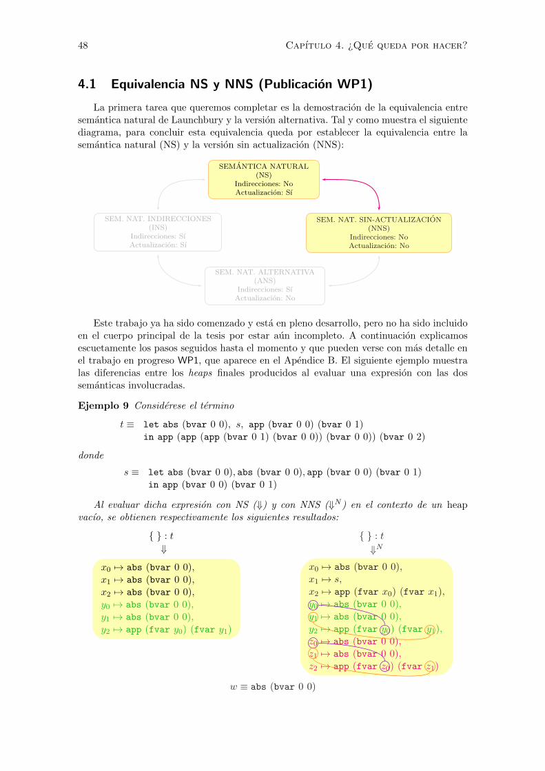
48 Capıtulo 4. ¿Que queda por hacer?
4.1 Equivalencia NS y NNS (Publicacion WP1)
La primera tarea que queremos completar es la demostracion de la equivalencia entresemantica natural de Launchbury y la version alternativa. Tal y como muestra el siguientediagrama, para concluir esta equivalencia queda por establecer la equivalencia entre lasemantica natural (NS) y la version sin actualizacion (NNS):
SEMANTICA NATURAL(NS)
Indirecciones: NoActualizacion: Sı
SEM. NAT. INDIRECCIONES(INS)
Indirecciones: SıActualizacion: Sı
SEM. NAT. SIN-ACTUALIZACION(NNS)
Indirecciones: NoActualizacion: No
SEM. NAT. ALTERNATIVA(ANS)
Indirecciones: SıActualizacion: No
Este trabajo ya ha sido comenzado y esta en pleno desarrollo, pero no ha sido incluidoen el cuerpo principal de la tesis por estar aun incompleto. A continuacion explicamosescuetamente los pasos seguidos hasta el momento y que pueden verse con mas detalle enel trabajo en progreso WP1, que aparece en el Apendice B. El siguiente ejemplo muestralas diferencias entre los heaps finales producidos al evaluar una expresion con las dossemanticas involucradas.
Ejemplo 9 Considerese el termino
t ≡ let abs (bvar 0 0), s, app (bvar 0 0) (bvar 0 1)in app (app (app (bvar 0 1) (bvar 0 0)) (bvar 0 0)) (bvar 0 2)
donde
s ≡ let abs (bvar 0 0), abs (bvar 0 0), app (bvar 0 0) (bvar 0 1)in app (bvar 0 0) (bvar 0 1)
Al evaluar dicha expresion con NS (⇓) y con NNS (⇓N ) en el contexto de un heapvacıo, se obtienen respectivamente los siguientes resultados:
{ } : t
⇓
x0 7→ abs (bvar 0 0),x1 7→ abs (bvar 0 0),x2 7→ abs (bvar 0 0),y0 7→ abs (bvar 0 0),y1 7→ abs (bvar 0 0),y2 7→ app (fvar y0) (fvar y1)
{ } : t
⇓N
x0 7→ abs (bvar 0 0),x1 7→ s,
x2 7→ app (fvar x0) (fvar x1),y0 7→ abs (bvar 0 0),y1 7→ abs (bvar 0 0),y2 7→ app (fvar y0) (fvar y1),z0 7→ abs (bvar 0 0),z1 7→ abs (bvar 0 0),z2 7→ app (fvar z0) (fvar z1)
w ≡ abs (bvar 0 0)
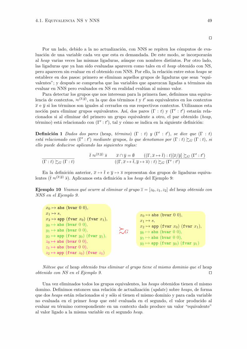
4.1. Equivalencia NS y NNS 49
ut
Por un lado, debido a la no actualizacion, con NNS se repiten los computos de eva-luacion de una variable cada vez que esta es demandada. De este modo, se incorporaranal heap varias veces las mismas ligaduras, aunque con nombres distintos. Por otro lado,las ligaduras que ya han sido evaluadas aparecen como tales en el heap obtenido con NS,pero aparecen sin evaluar en el obtenido con NNS. Por ello, la relacion entre estos heaps seestablece en dos pasos: primero se eliminan aquellos grupos de ligaduras que sean “equi-valentes”; y despues se comprueba que las variables que aparezcan ligadas a terminos sinevaluar en NNS pero evaluados en NS en realidad evaluan al mismo valor.
Para detectar los grupos que nos interesan para la primera fase, definimos una equiva-lencia de contextos, ≈(x,y), en la que dos terminos t y t′ son equivalentes en los contextosx e y si los terminos son iguales al cerrarlos en sus respectivos contextos. Utilizamos estanocion para eliminar grupos equivalentes. Ası, dos pares (Γ : t) y (Γ′ : t′) estaran rela-cionados si al eliminar del primero un grupo equivalente a otro, el par obtenido (heap,termino) esta relacionado con (Γ′ : t′), tal y como se indica en la siguiente definicion:
Definicion 1 Dados dos pares (heap, termino) (Γ : t) y (Γ′ : t′), se dice que (Γ : t)esta relacionado con (Γ′ : t′) mediante grupos, lo que denotamos por (Γ : t) %G (Γ : t), siello puede deducirse aplicando las siguientes reglas:
(Γ : t) %G (Γ : t)
t ≈(x,y) s x ∩ y = ∅ ((Γ, x 7→ t) : t)[x/y] %G (Γ′ : t′)
((Γ, x 7→ t, y 7→ s) : t) %G (Γ′ : t′)
En la definicion anterior, x 7→ t e y 7→ s representan dos grupos de ligaduras equiva-lentes (t ≈(x,y) s). Aplicamos esta definicion a los heap del Ejemplo 9:
Ejemplo 10 Veamos que ocurre al eliminar el grupo z = [z0, z1, z2] del heap obtenido conNNS en el Ejemplo 9.
x0 7→ abs (bvar 0 0),x1 7→ s,
x2 7→ app (fvar x0) (fvar x1),y0 7→ abs (bvar 0 0),y1 7→ abs (bvar 0 0),y2 7→ app (fvar y0) (fvar y1),z0 7→ abs (bvar 0 0),z1 7→ abs (bvar 0 0),z2 7→ app (fvar z0) (fvar z1)
%G
x0 7→ abs (bvar 0 0),x1 7→ s,
x2 7→ app (fvar x0) (fvar x1),y0 7→ abs (bvar 0 0),y1 7→ abs (bvar 0 0),y2 7→ app (fvar y0) (fvar y1)
Notese que el heap obtenido tras eliminar el grupo tiene el mismo dominio que el heapobtenido con NS en el Ejemplo 9. ut
Una vez eliminados todos los grupos equivalentes, los heaps obtenidos tienen el mismodomino. Definimos entonces una relacion de actualizacion (update) sobre heaps, de formaque dos heaps estan relacionados si y solo si tienen el mismo dominio y para cada variableno evaluada en el primer heap que este evaluada en el segundo, el valor producido alevaluar su termino correspondiente en un contexto dado produce un valor “equivalente”al valor ligado a la misma variable en el segundo heap.
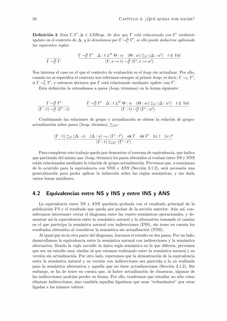
50 Capıtulo 4. ¿Que queda por hacer?
Definicion 2 Sean Γ,Γ′,∆ ∈ LNHeap. Se dice que Γ esta relacionado con Γ′ medianteupdate en el contexto de ∆, y lo denotamos por Γ ∼∆
U Γ′, si ello puede deducirse aplicandolas siguientes reglas:
Γ ∼∆U Γ
Γ ∼∆U Γ′ ∆ : t ⇓N Θ : w (Θ : w) %G (∆ : w′) t /∈ Val
(Γ, x 7→ t) ∼∆U (Γ′, x 7→ w′)
Nos interesa el caso en el que el contexto de evaluacion es el heap sin actualizar. Por ello,cuando no se especifica el contexto nos referimos siempre al primer heap; es decir, Γ ∼U Γ′,si Γ ∼Γ
U Γ′, y entonces decimos que Γ esta relacionado mediante update con Γ′.
Esta definicion la extendemos a pares (heap, terminos) en la forma siguiente:
Γ ∼∆U Γ′
(Γ : t) ∼∆U (Γ′ : t)
Γ ∼∆U Γ′ ∆ : t ⇓N Θ : w (Θ : w) %G (∆ : w′) t /∈ Val
(Γ : t) ∼∆U (Γ′ : w′)
Combinando las relaciones de grupo y actualizacion se obiene la relacion de grupo-actualizacion sobre pares (heap, termino), %GU :
(Γ : t) %G (∆ : s) (∆ : s) ∼U (Γ′ : t′) ok Γ ok Γ′ lc t lc t′
(Γ : t) %GU (Γ′ : t′)
Para completar este trabajo queda por demostrar el teorema de equivalencia, que indicaque partiendo del mismo par (heap, termino) los pares obtenidos al evaluar entre NS y NNSestan relacionados mediante la relacion de grupo-actualizacion. Prevemos que, a semejanzade lo ocurrido para la equivalencia con NNS y ANS (Seccion 3.1.2), sera necesaria unageneralizacion para poder aplicar la induccion sobre las reglas semanticas, y sin dudavarios lemas auxiliares.
4.2 Equivalencias entre NS y INS y entre INS y ANS
La equivalencia entre NS y ANS quedarıa probada con el resultado principal de lapublicacion P3 y el resultado que queda por probar de la seccion anterior. Aun ası, con-sideramos interesante cerrar el diagrama entre las cuatro semanticas operacionales, y de-mostrar ası la equivalencia entre la semantica natural y la alternativa tomando el caminoen el que participa la semantica natural con indirecciones (INS), sin tener en cuenta losresultados obtenidos al considerar la semantica sin actualizacion (NNS).
Al igual que en la otra parte del diagrama, haremos el estudio en dos pasos. Por un lado,desarrollamos la equivalencia entre la semantica natural con indirecciones y la semanticaalternativa. Siendo la regla variable la unica regla semantica en la que difieren, prevemosque sea un estudio muy similar al que estamos realizando entre la semantica natural y suversion sin actualizacion. Por otro lado, esperamos que la demostracion de la equivalenciaentre la semantica natural y su version con indirecciones sea parecida a la ya realizadapara la semantica alternativa y aquella que no tiene actualizaciones (Seccion 3.1.2). Sinembargo, se ha de tener en cuenta que, al haber actualizacion de clausuras, algunas delas indirecciones podrıan perder su forma. Por ello, tendremos que estudiar no solo comoeliminar indirecciones, sino tambien aquellas ligaduras que sean “redundantes” por estarligadas a los mismos valores.
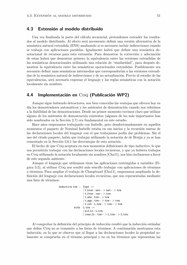
4.3. Extension al modelo distribuido 51
4.3 Extension al modelo distribuido
Una vez finalizada la parte del calculo secuencial, pretendemos extender los resulta-dos al modelo distribuido. Al efecto sera neceserario definir una version alternativa de lasemantica natural extendida (ENS) analizando si es necesario incluir indirecciones cuandose trabaja con aplicaciones paralelas. Igualmente habra que definir una semantica de-notacional de recursos para esta extension. Para demostrar la correccion y adecuacionde estas habra que demostrar primero la equivalencia entre las versiones extendidas delas semanticas denotacionales utilizando una relacion de “similaridad”, para despues de-mostrar la equivalencia entre las semanticas operacionales extendidas. Posiblemente seanecesario definir unas semanticas intermedias que corresponderıan a las versiones extendi-das de la semantica natural de indirecciones y de no actualizacion. Previo al estudio de lasequivalencias, sera necesario expresar el lenguaje y las reglas semanticas con la notacionlocalmente sin nombres.
4.4 Implementacion en Coq (Publicacion WP2)
Aunque sigue habiendo detractores, son bien conocidas las ventajas que ofrecen hoy endıa los demostradores automaticos y los asistentes de demostracion cuando nos referimosa la fiabilidad de las demostraciones. Desde un primer momento tuvimos claro que utilizaralguno de los asistentes de demostracion existentes (algunos de los mas importantes hansido nombrados en la Seccion 2.7) era fundamental en este estudio.
Hace anos empezamos trabajando con Isabelle, pero desafortunadamente en aquellosmomentos el paquete de Nominal Isabelle estaba en sus inicios y la recursion mutua delas declaraciones locales del lenguaje con el que trabajamos podıa dar problemas. Sin eluso del citado paquete, habıa que trabajar utilizando la notacion de de Bruijn y ya se hancomentado en la Seccion 2.6.1 las desventajas de esta notacion.
El hecho de que Coq aceptara en esos momentos definiciones de tipo inductivo, lo quenos permitirıa trabajar con las declaraciones locales recursivas, y que ya hubiera trabajosen Coq utilizando la notacion localmente sin nombres [Cha11], nos hizo inclinarnos a favorde este segundo asistente.
Aunque el lenguaje que utilizamos tiene las aplicaciones restringidas a variables (Fi-gura 3.2), al utilizar Coq nos resulto mas sencillo trabajar con aplicaciones de terminosa terminos. Para ampliar el trabajo de Chargeraud [Cha11], empezamos ampliando la de-finicion del lenguaje con declaraciones locales recursivas, que son representadas medianteuna lista de terminos:
Inductive trm : Type :=| t bvar : nat− > nat− > trm
| t fvar : var− > trm
| t abs : trm− > trm
| t app : trm− > trm− > trm
| t let : L trm− > trm− > trm
with L trm :=| nil Lt : L trm
| cons Lt : trm− > L trm− > L trm.
Al comprobar la definicion del principio de induccion resulto que la induccion estandarque define Coq no se transmite a las listas de terminos. A continuacion mostramos estainduccion, en la que se observa que al llegar a las declaraciones locales la propiedad so-lamente se comprueba en el termino principal y no en los terminos que representan las
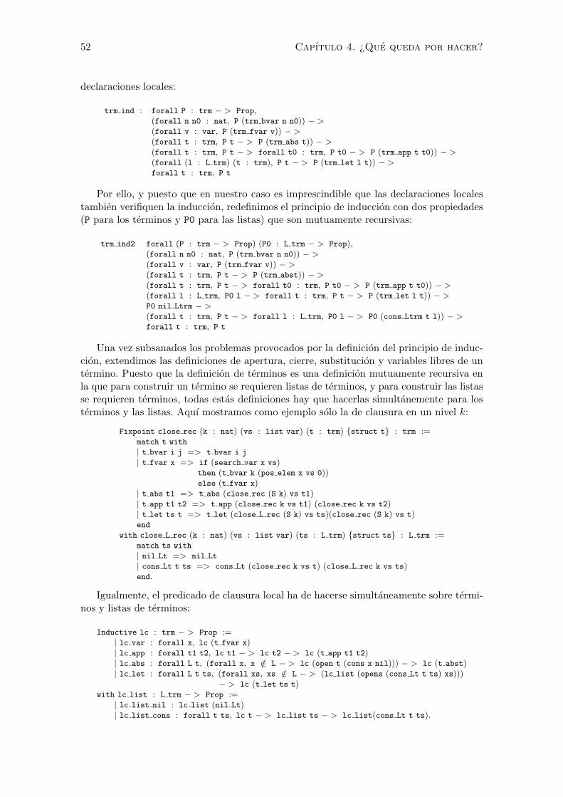
52 Capıtulo 4. ¿Que queda por hacer?
declaraciones locales:
trm ind : forall P : trm − > Prop,(forall n n0 : nat, P (trm bvar n n0)) − >(forall v : var, P (trm fvar v)) − >(forall t : trm, P t − > P (trm abs t)) − >(forall t : trm, P t − > forall t0 : trm, P t0 − > P (trm app t t0)) − >(forall (l : L trm) (t : trm), P t − > P (trm let l t)) − >forall t : trm, P t
Por ello, y puesto que en nuestro caso es imprescindible que las declaraciones localestambien verifiquen la induccion, redefinimos el principio de induccion con dos propiedades(P para los terminos y P0 para las listas) que son mutuamente recursivas:
trm ind2 forall (P : trm − > Prop) (P0 : L trm − > Prop),(forall n n0 : nat, P (trm bvar n n0)) − >(forall v : var, P (trm fvar v)) − >(forall t : trm, P t − > P (trm abst)) − >(forall t : trm, P t − > forall t0 : trm, P t0 − > P (trm app t t0)) − >(forall l : L trm, P0 l − > forall t : trm, P t − > P (trm let l t)) − >P0 nil Ltrm − >(forall t : trm, P t − > forall l : L trm, P0 l − > P0 (cons Ltrm t l)) − >forall t : trm, P t
Una vez subsanados los problemas provocados por la definicion del principio de induc-cion, extendimos las definiciones de apertura, cierre, substitucion y variables libres de untermino. Puesto que la definicion de terminos es una definicion mutuamente recursiva enla que para construir un termino se requieren listas de terminos, y para construir las listasse requieren terminos, todas estas definiciones hay que hacerlas simultanemente para losterminos y las listas. Aquı mostramos como ejemplo solo la de clausura en un nivel k:
Fixpoint close rec (k : nat) (vs : list var) (t : trm) {struct t} : trm :=match t with
| t bvar i j => t bvar i j
| t fvar x => if (search var x vs)then (t bvar k (pos elem x vs 0))else (t fvar x)
| t abs t1 => t abs (close rec (S k) vs t1)| t app t1 t2 => t app (close rec k vs t1) (close rec k vs t2)| t let ts t => t let (close L rec (S k) vs ts)(close rec (S k) vs t)end
with close L rec (k : nat) (vs : list var) (ts : L trm) {struct ts} : L trm :=match ts with
| nil Lt => nil Lt
| cons Lt t ts => cons Lt (close rec k vs t) (close L rec k vs ts)end.
Igualmente, el predicado de clausura local ha de hacerse simultaneamente sobre termi-nos y listas de terminos:
Inductive lc : trm − > Prop :=| lc var : forall x, lc (t fvar x)| lc app : forall t1 t2, lc t1 − > lc t2 − > lc (t app t1 t2)| lc abs : forall L t, (forall x, x /∈ L − > lc (open t (cons x nil))) − > lc (t abst)| lc let : forall L t ts, (forall xs, xs /∈ L − > (lc list (opens (cons Lt t ts) xs)))
− > lc (t let ts t)with lc list : L trm − > Prop :=
| lc list nil : lc list (nil Lt)| lc list cons : forall t ts, lc t − > lc list ts − > lc list(cons Lt t ts).
4.4. Implementacion en Coq 53
Posteriormente avanzamos definiendo las ligaduras, los heaps, funciones sobre los heaps(como el dominio, los nombres, la sustitucion de nombres y el predicado de heaps bien de-finidos comentados en la Seccion 3.1.2). Aun ası, estas definiciones tienen que ser revisadasya que parece que no son las mas adecuadas para la definicion de las reglas semanticas y lasposteriores demostraciones. La definicion de heap se ha dado como conjunto de ligaduras,pero algunos expertos en Coq nos han indicado que quiza serıa mas conveniente hacer-lo mediante una funcion parcial. Por ello habra que indagar las diferencias entre ambasdefiniciones y las ventajas e inconvenientes que pueda tener cada metodo.
Esta parte de la investigacion ha sido aplazada para ser retomada posteriormente.Trabajar con asistentes de demostracion es complejo y demostraciones que en lapiz ypapel parecen sencillas, pueden convertirse en algo muy complicado. Era imprescindiblededicarle un tiempo del que no disponıamos en el momento en el que se comenzo a elaborareste trabajo y que esperamos poder tener en el futuro. Por ello, al igual que la publicacionWP1 descrita en la Seccion 4.1, WP2 no forma parte del nucleo de la tesis.
Ciertamente aun queda camino por recorrer pero lo ya hecho y expuesto en el Capıtulo 3tiene la suficiente entidad (unidad, dificultad, volumen, claridad y representatividad) comopara dar lugar a la Tesis doctoral que presentamos aquı.

54 Capıtulo 4. ¿Que queda por hacer?
Part II
Summary of the Research
55


Chapter 1
What, why and how?
When several semantics are defined for a programming language, these semanticsshould be equivalent, in the sense that equivalent meanings are given for each programwritten in the language. Hidalgo-Herrero, in her PhD thesis [Hid04], defined an opera-tional and a denotational semantics for Jauja, a simplification of Eden [BLOP96]. Thislanguage has two differentiated parts:
a lazy λ-calculus; and
coordination expressions.
The initial purpose of this thesis was to prove the equivalence between the seman-tics defined by Hidalgo-Herrero. But this goal turned out to be too ambitious, since thecoordination expressions of Jauja complicated considerably the task of proving the equiv-alence between a small-step operational semantics and a continuation-based denotationalsemantics. Therefore, the final target of this thesis is to give the first steps in proving thedesired equivalence.
For a start, we have based our work on Launchbury’s ideas [Lau93] to prove theequivalence between a big step natural semantics and a standard denotational semanticsdefined for a λ-calculus extended with local declarations. We have extended the λ-calculusused by Launchbury with a parallel application. This expression gives rise to the creationof new processes and the communication between them. In order to define the meaningof the new expression and the new identifiers (for channels) we have extended the naturalsemantics. These extensions had to be consistent with Launchbury’s and with Hidalgo-Herrero’s definitions.
We can differentiate two parts in this thesis: one is dedicated to a distributed modelformed by several processes that interact between them; the other part focuses on a oneprocessor model.
Paradoxically, the study of the distributed model has led to a deeper examination ofthe one processor model, where we have two parts: in the first one we studied the charac-teristics and relations between denotational semantics; in the second one we analyzed theproperties and relations of several operational semantics.
During the research we have found a number of problems that we have solved. Someparts of this thesis are the consequence of the absence of detailed proofs in [Lau93]. Al-though Launchbury gave some intuitive ideas, its development is more complex than ex-pected and rule induction is insufficient. Since several works for some results [BKT00,HO02, NH09, Ses97, vEdM07] are based on Launchbury’s study, we considered very im-portant to formalize those results.
57

58 Chapter 1. What, why and how?
The notation for representing the expressions of a language can facilitate or complicatethe formalization of proofs. Working with a λ-calculus usually gives problems relatedwith the α-conversion. Several techniques have been developed to avoid them: the deBruijn notation [dB72], the locally nameless representation [Cha11] or the techniques ofthe nominal logic [Pit13]. We have worked with the second option in some of the articlesthat form this thesis.
Summarizing, we have studied different semantics and techniques for the representationof terms of a λ-calculus with local declarations in order to establish the equivalence betweensome semantics of a distributed model.
1.1 Objectives
The main purpose of this thesis is:
to begin with the proof of the equivalence between the semantics for Jauja givenin [Hid04].
In order to achieve this, we focus on the following targets:
to extend the λ-calculus with a parallel application, i.e., to introduce explicit paral-lelism;
to define for this extension different operational and denotational semantic models(for one and for several processors);
to study the relation between the defined semantic models, that is, to formalize theequivalence between the semantics defined in the previous step;
to formalize the missing proofs in [Lau93], particularly the equivalence between astandard denotational semantics and a resourced denotational semantics, and be-tween Launchbury’s natural semantics and its alternative version.
1.2 Summary
This thesis is composed by a collection of publications. In order to understand therelation between these publications and to facilitate its reading, we have written thisintroduction and three additional chapters. We explain in Chapter 2 some preliminaryconcepts useful to understand the material presented in the publications. Chapter 3is dedicated to the obtained results. All these results are detailed in the publications,therefore the purpose of this chapter is only to give an intuitive idea of them. Each sectionof the chapter is related with one or more publications, and this is explicity indicated.We also show in this chapter some of the related work. Future work is presented inChapter 4. This is divided in four sections where we explain different future research linesand how much we have already done. Finally, Chapter 5 includes the main publicationsthat compose the thesis:
P1: Relating function spaces to resourced function spaces [SGHHOM11].
P2: A Locally Nameless Representation for a Natural Semantics for Lazy Evalua-tion [SGHHOM12b].
P3: The Role of Indirections in Lazy Natural Semantics [SGHHOM14b].

1.2. Summary 59
P4: An Operational Semantics for Distributed Lazy Evaluation [SGHHOM10].
We have included two appendices. Appendix A contains two technical reports with ex-tended versions of publications P2 and P3. In these extensions can be found detailedproofs of the results in the corresponding publications.
TR1: A locally nameless representation for a natural semantics for lazy evalua-tion [SGHHOM12c].
TR2: The role of indirections in lazy natural semantics [SGHHOM13].
To conclude, we show two works in progress in Appendix B. First steps have been com-pleted on these works, but further development has been postponed for several reasons:
WP1: Launchbury’s semantics revisited: On the equivalence of context-heap seman-tics [SGHHOM14a].
WP2: A formalization in Coq of Launchbury’s natural semantics for lazy evalua-tion [SGHHOM12a].

60 Chapter 1. What, why and how?

Chapter 2
What was done?
We explain in this chapter some concepts developed by others and that are used inthis thesis.
2.1 Programming languages
Every language is composed by a syntax and a semantics. The syntax shows how tobuild correct expressions, while the semantics gives meaning to them. This applies also toprogramming languages: the syntax determines how to build programs, and the semanticsexpresses how they behave when they are executed in a computer.
In the case of programming languages, formal semantics prevent ambiguities, i.e., eachterm has a unique meaning.
2.1.1 Functional Programming Languages
There are several programming paradigms. In the imperative one programmers definestep by step how to solve a problem even when the procedure differs from the initial math-ematical definition. Functional programming languages have a higher level of abstraction.
Let us consider a simple example. The mathematical definition to calculate the nth
power of a number is:
x0 = 1xn+1 = x · xn
In an imperative language as C the expression to represent the nth power is:
int power(int x, int n);{
int i = 1;int result = 1;while (i <= n){
result = result ∗ x;i+ +;
}return(result);
}While in a functional language like Haskell, the definition is:
61
62 Chapter 2. What was done?
power x 0 = 1power x n = x ∗ power x (n− 1)
Usually functional programming languages are considered to be less efficient than im-perative ones. Barendregt and Barendsen explain in [BB00] that Von-Neumann archi-tecture is based on the Turing machine. Imperative programming languages follow asequence of instructions that are close to this architecture. However, functional program-ming languages are more efficient in reduction machines, which are created to executethese languages based in the λ-calculus. The lost of efficiency of functional program-ming languages is due to the fact that most computers have a Von-Neumann architecture.For this reason, lots of studies about functional languages have been devoted to developefficient implementations of functional programming languages, and nowadays the execu-tion time of these languages is competitive. Moreover, functional languages offer someadvantages such as a higher level of abstraction, a shorter code, no side effects, easy de-bugging, concurrency, hot code deployment, natural recursion, etc. Thus, at the presenttime functional programming is not only restricted to the academic context. For instanceHaskell is used in Intel, Deutsche Bank and even in Facebook and Google [has14a], whileErlang [erl14a] is used in Whatsapp [wha14], Facebook and T-Mobile [erl14b].
2.1.2 Evaluation strategies
Expressions in functional programming languages are evaluated by the reduction ofsubexpressions. Depending on the reduction order of redexes (reduction expressions),different evaluation strategies are obtained. They can be classified into two groups: thefirst one refers to those strategies where the evaluation of arguments is done before applyingthe function although they may not be required (eager evaluation); the second one refersto the strategies where the arguments are only evaluated if they are needed to continuewith the computation (lazy evaluation).
In this thesis we use the following evaluation strategies (as defined in [Rea89]):
Call-by-value: It is an eager strategy where the arguments are evaluated before thefunction’s body;
Call-by-name: It is an strategy of the second group where the argument (that has notbeen evaluated) is replaced in the function’s body which is then evaluated. Althoughsome expressions may be evaluated several times, if they are not required, they willnot be evaluated at all;
Call-by-need : It is a lazy strategy but more efficient than call-by-name since thevalue of an expression is stored and shared. Therefore, expressions are evaluated atmost once.
2.1.3 Parallel functional languages
The development of parallel and distributed machines leads to the search of program-ming languages that facilitate parallel programming. Imperative languages are useful forthis purpose, but synchronization and communication are treated in a very low level ofabstraction. By contrast, functional languages present some advantages, as we have seenin Section 2.1.1.
Loogen [Loo99] classifies the parallelism in functional programming languages intothree groups, depending on the allowance of the programmer to establish where parallelismhas to be performed:

2.1. Programming languages 63
Implicit parallelism: This is inherent in the reduction semantics. Independent re-dexes can be reduced in an arbitrary order. Therefore, they can be reduced inparallel. It is related to the automatic parallelization of functional programminglanguages.
Controlled parallelism: The programmer adds some annotations indicating to thecompiler where parallelism could be performed. High level parallel constructions areused, such as skeletons [Col89] or evaluation strategies [THLP98].
Explicit parallelism: The programmer establishes which expressions must be com-puted in parallel. Some languages, such as Haskell [Pey03] or ML [MTH90], haveextensions to deal with explicit process creation, communication and synchronizationbetween processes.
The functional programming language Haskell [Pey03, has14b] has been the origin ofseveral parallel and distributed versions [TLP03]. Haskell follows a lazy evaluation strat-egy (Section 2.1.2); since expressions are evaluated under demand, parallelism is restricted.The parallel versions of Haskell eliminate some laziness either by speculative computa-tions, i.e., allowing the evaluation of non-demanded parts (for instance in GpH [THLP98]with the operator par), or by introducing strictness, i.e., forcing the evaluation of ex-pressions before the result is needed (for instance the operator seq in GpH [THLP98]).
2.1.4 The functional parallel language Eden
This thesis focuses on some properties of the kernel of the functional parallel languageEden [BLOP96, LOP05, ede14]. Eden is an extension of Haskell with some syntacticconstructs for explicit process specification and creation, which provide enough control toimplement parallel algorithms. It also introduces automatic communication via streams.The main characteristics of Eden are:
Process abstractions: Expressions that define the general behavior of a process in afunctional way.
Process creations: Applications of the process abstractions to a group of expressions.These expressions produce the values of the input channels of the new process.
Communication between processes: It is asynchronous and implicit, since the trans-mission of messages is not explicitly made by the programmer. Communications canbe of just one value, or of several values through a stream.
The constructions of Eden also model reactive systems:
Dynamic channel creation: This allows to break the hierarchy between processes.That is, in addition to communications between father and child processes, they arealso between any pair of processes.
Non-determinism: To model many-to-one communications, a special process ab-straction merges several streams into one in a non-deterministic way.
64 Chapter 2. What was done?
2.2 Programming Language Semantics
In the preface of [Win93], Winskel explains that giving a formal semantics to a pro-gramming language lies in building a mathematical model. Formal semantics allow us tounderstand and to reason about programs behavior.
2.2.1 Formal semantics
There are different types of formal semantics. In this thesis we use two types of them:
Operational: An operational semantics describes the meaning of a program interms of how it is executed by an abstract machine. It focuses on both the finalvalue and how this value is obtained. They are classified into two groups: smallstep semantics, which detail how computations are performed step by step, and bigstep semantics or natural semantics, which describe how the final value is directlyobtained.
Denotational: A denotational semantics gives meaning to programs throughmathematical objects, which are called denotations. For its definition, the first taskis to find some mathematical object representing the effect of a program. So that thesemantics describes the function computed by the program, but it is not concernedin how this is done. The denotation of a term is obtained by the composition of thedenotations of the subterms. This semantics has a higher level of abstraction thanthe operational semantics, and hence it is useful to study the equivalence betweenprograms. The steps to define a denotational semantics are: to define a space ofmeanings, to give to each constant of the language a meaning in this space, to definefor each constructor in the language a semantic function over the space of meanings,and finally, to define the main semantic function corresponding to the semantic valueof each program.
When two (or more) formal semantics are defined for the same language, it mustbe proved that they are equivalent. When dealing with operational and denotationalsemantics, this equivalence is usually expressed in terms of correctness and computationaladequacy:
Correctness: An operational semantics is correct with respect to a denotationalone, if the operational reduction preserves the denotational meaning of terms andonly the meaning of the contexts of evaluation is modified.
Computational adequacy: The computational adequacy of an operational se-mantics with respect to a denotational semantics establishes that whenever the de-notation of some term is defined then there exists an operational reduction for thisterm.
In this thesis we work with several operational and denotational semantics of a func-tional programming language, and we study the relation between them.
2.3 Function spaces
As it is explained in [Win93], comparing programs that are written in different pro-gramming languages can be very complex if operational semantics are involved. Thereason is that they deeply depend on the syntax of the language. However, denotational
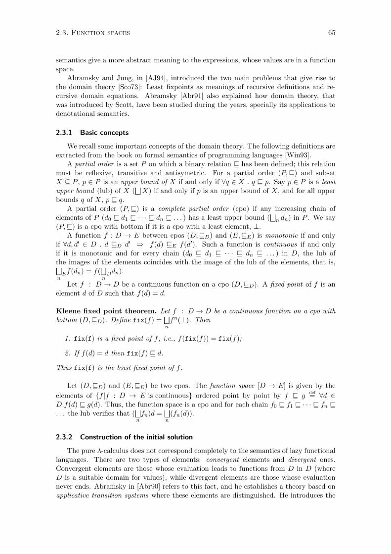
2.3. Function spaces 65
semantics give a more abstract meaning to the expressions, whose values are in a functionspace.
Abramsky and Jung, in [AJ94], introduced the two main problems that give rise tothe domain theory [Sco73]: Least fixpoints as meanings of recursive definitions and re-cursive domain equations. Abramsky [Abr91] also explained how domain theory, thatwas introduced by Scott, have been studied during the years, specially its applications todenotational semantics.
2.3.1 Basic concepts
We recall some important concepts of the domain theory. The following definitions areextracted from the book on formal semantics of programming languages [Win93].
A partial order is a set P on which a binary relation v has been defined; this relationmust be reflexive, transitive and antisymetric. For a partial order (P,v) and subsetX ⊆ P , p ∈ P is an upper bound of X if and only if ∀q ∈ X . q v p. Say p ∈ P is a leastupper bound (lub) of X (
⊔X) if and only if p is an upper bound of X, and for all upper
bounds q of X, p v q.A partial order (P,v) is a complete partial order (cpo) if any increasing chain of
elements of P (d0 v d1 v · · · v dn v . . . ) has a least upper bound (⊔n dn) in P . We say
(P,v) is a cpo with bottom if it is a cpo with a least element, ⊥.A function f : D → E between cpos (D,vD) and (E,vE) is monotonic if and only
if ∀d, d′ ∈ D . d vD d′ ⇒ f(d) vE f(d′). Such a function is continuous if and onlyif it is monotonic and for every chain (d0 v d1 v · · · v dn v . . . ) in D, the lub ofthe images of the elements coincides with the image of the lub of the elements, that is,⊔E
nf(dn) = f(
⊔D
ndn).
Let f : D → D be a continuous function on a cpo (D,vD). A fixed point of f is anelement d of D such that f(d) = d.
Kleene fixed point theorem. Let f : D → D be a continuous function on a cpo withbottom (D,vD). Define fix(f) =
⊔nfn(⊥). Then
1. fix(f) is a fixed point of f , i.e., f(fix(f)) = fix(f);
2. If f(d) = d then fix(f) v d.
Thus fix(f) is the least fixed point of f .
Let (D,vD) and (E,vE) be two cpos. The function space [D → E] is given by the
elements of {f |f : D → E is continuous} ordered point by point by f v gdef= ∀d ∈
D.f(d) v g(d). Thus, the function space is a cpo and for each chain f0 v f1 v · · · v fn v. . . the lub verifies that (
⊔nfn)d =
⊔n
(fn(d)).
2.3.2 Construction of the initial solution
The pure λ-calculus does not correspond completely to the semantics of lazy functionallanguages. There are two types of elements: convergent elements and divergent ones.Convergent elements are those whose evaluation leads to functions from D in D (whereD is a suitable domain for values), while divergent elements are those whose evaluationnever ends. Abramsky in [Abr90] refers to this fact, and he establishes a theory based onapplicative transition systems where these elements are distinguished. He introduces the
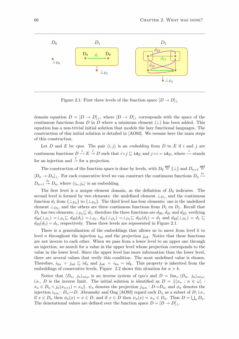
66 Chapter 2. What was done?
⊥D0
D0
D0 D0
D1
⊥D1
d1
D2
⊥D2
d21
d20
d22
Figure 2.1: First three levels of the function space [D → D]⊥
domain equation D = [D → D]⊥, where [D → D]⊥ corresponds with the space of thecontinuous functions from D in D where a minimum element (⊥) has been added. Thisequation has a non-trivial initial solution that models the lazy functional languages. Theconstruction of this initial solution is detailed in [AO93]. We resume here the main stepsof this construction.
Let D and E be cpos. The pair 〈i, j〉 is an embedding from D to E if i and j are
continuous functions Di� E
j� D such that i ◦ j v idE and j ◦ i = idD, where
i� stands
for an injection andj� for a projection.
The construction of the function space is done by levels, with D0def= {⊥} and Dn+1
def=
[Dn → Dn]⊥. For each consecutive level we can construct the continuous functions Dnin�
Dn+1
jn� Dn, where 〈in, jn〉 is an embedding.
The first level is a unique element domain, as the definition of D0 indicates. Thesecond level is formed by two elements: the undefined element ⊥D1 , and the continuousfunction d1 from {⊥D0} to {⊥D0}. The third level has four elements: one is the undefinedelement ⊥D2 , and the others are three continuous functions from D1 en D1. Recall thatD1 has two elements, ⊥D1v d1, therefore the three functions are d20, d21 and d22, verifyingd20(⊥D1) =⊥D1v d20(d1) =⊥D1 , d21(⊥D1) =⊥D1v d21(d1) = d1 and d22(⊥D1) = d1 vd22(d1) = d1, respectively. These three levels are represented in Figure 2.1.
There is a generalization of the embeddings that allows us to move from level k tolevel n throughout the injection ikn and the projection jnk. Notice that these functionsare not inverse to each other. When we pass from a lower level to an upper one throughan injection, we search for a value in the upper level whose projection corresponds to thevalue in the lower level. Since the upper level has more information than the lower level,there are several values that verify this condition. The most undefined value is chosen.Therefore, ikn ◦ jnk v idn and jnk ◦ ikn = idk. This property is inherited from theembeddings of consecutive levels. Figure 2.2 shows this situation for n > k.
Notice that 〈Dn, jn〉n∈ω is an inverse system of cpo’s and D = lim←〈Dn, jn〉n∈ω,i.e., D is the inverse limit. The initial solution is identified as D = {〈xn : n ∈ ω〉 :xn ∈ Dn ∧ jn(xn+1) = xn}. ψn denotes the projection j∞n : D�Dn, and φn denotes theinjection in∞ : Dn�D. Abramsky and Ong [AO93] regard each Dn as a subset of D; i.e.,if x ∈ Dn then φn(x) = x ∈ D, and if x ∈ D then ψn(x) = xn ∈ Dn. Thus D =
⋃nDn.
The denotational values are defined over the function space D = [D → D]⊥.

2.3. Function spaces 67
...
...
Dn
⊥Dn
...
Dk
⊥Dk
iknjnk
Figure 2.2: Injections and projections between levels
λx.P ⇓ λx.PM ⇓ λx.P P [x := Q] ⇓ N
M Q ⇓ N
Figure 2.3: Binary relation in Λ0
2.3.3 Applicative bisimulation
To explain the concept of applicative bisimulation defined in [Abr90], we consider aλ-calculus where the closed λ-terms, represented by Λ0, stand for programs and the λ-abstractions for values. A binary relation ⇓ ⊆ Λ0 × Λ0 is defined, and its rules are shownin Figure 2.3. A term M converges, denoted by M ⇓, if there exists a term N suchthat M ⇓ N , and a term M diverges otherwise. That is, a term either converges to aλ-abstraction, or diverges.
This definition is the basis for the applicative bisimulation. Abramsky and Ongin [AO93] explain that to determine the convergence of a term, one have to observe thebehavior of the term at each level. Let M be a closed term. In the first level we can onlysee if it converges to an abstraction λx.M1. If the answer is affirmative, we pass N1 asthe argument of the function and we observe if the obtained expression converges, i.e. ifM1[x := N1] is convergent. We keep on performing this once and again.
A sequence of binary relations, 〈vBk : k ∈ N〉, are defined over Λ0:
∀M,N . M vB0 N .
M vBk+1 Ndef= M ⇓ λx.P ⇒ (N ⇓ λx.Q ∧ ∀R ∈ Λ0.P [x := R] vBk Q[x := R]).
M vB Ndef= ∀k ∈ N . M vBk N .
Notice that at level 0 all the closed terms are related. We can only observe if a termreduces to a λ-abstraction, but the body of this λ-abstraction is not observable. Therefore,the only way to have some information about the body is to study how the function behaves
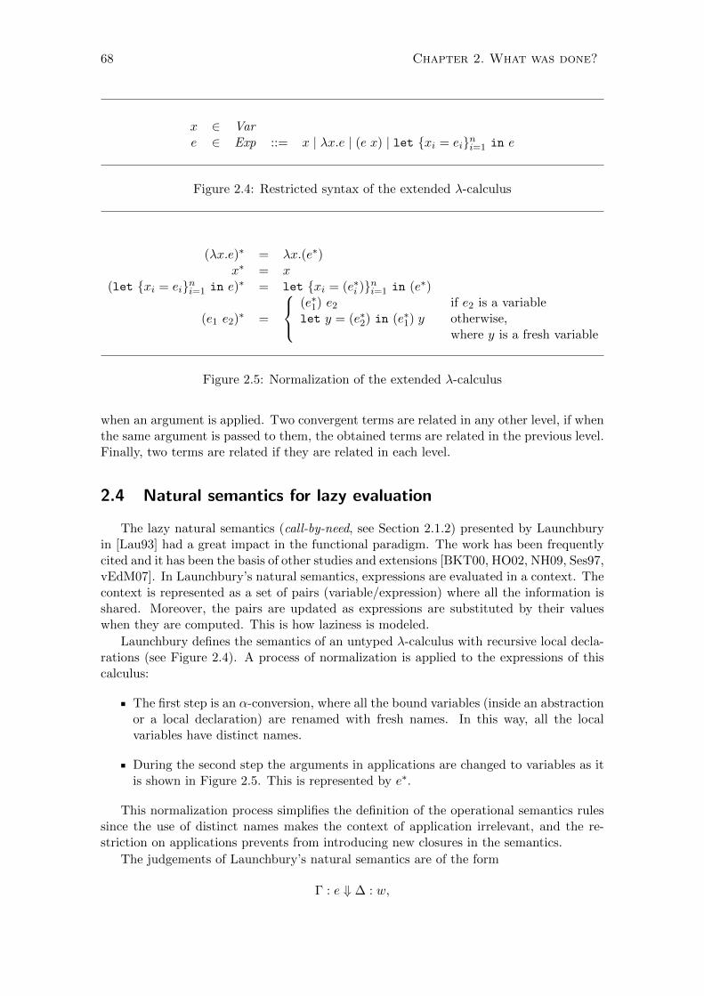
68 Chapter 2. What was done?
x ∈ Vare ∈ Exp ::= x | λx.e | (e x) | let {xi = ei}ni=1 in e
Figure 2.4: Restricted syntax of the extended λ-calculus
(λx.e)∗ = λx.(e∗)x∗ = x
(let {xi = ei}ni=1 in e)∗ = let {xi = (e∗i )}ni=1 in (e∗)
(e1 e2)∗ =
(e∗1) e2 if e2 is a variablelet y = (e∗2) in (e∗1) y otherwise,
where y is a fresh variable
Figure 2.5: Normalization of the extended λ-calculus
when an argument is applied. Two convergent terms are related in any other level, if whenthe same argument is passed to them, the obtained terms are related in the previous level.Finally, two terms are related if they are related in each level.
2.4 Natural semantics for lazy evaluation
The lazy natural semantics (call-by-need, see Section 2.1.2) presented by Launchburyin [Lau93] had a great impact in the functional paradigm. The work has been frequentlycited and it has been the basis of other studies and extensions [BKT00, HO02, NH09, Ses97,vEdM07]. In Launchbury’s natural semantics, expressions are evaluated in a context. Thecontext is represented as a set of pairs (variable/expression) where all the information isshared. Moreover, the pairs are updated as expressions are substituted by their valueswhen they are computed. This is how laziness is modeled.
Launchbury defines the semantics of an untyped λ-calculus with recursive local decla-rations (see Figure 2.4). A process of normalization is applied to the expressions of thiscalculus:
The first step is an α-conversion, where all the bound variables (inside an abstractionor a local declaration) are renamed with fresh names. In this way, all the localvariables have distinct names.
During the second step the arguments in applications are changed to variables as itis shown in Figure 2.5. This is represented by e∗.
This normalization process simplifies the definition of the operational semantics rulessince the use of distinct names makes the context of application irrelevant, and the re-striction on applications prevents from introducing new closures in the semantics.
The judgements of Launchbury’s natural semantics are of the form
Γ : e ⇓ ∆ : w,
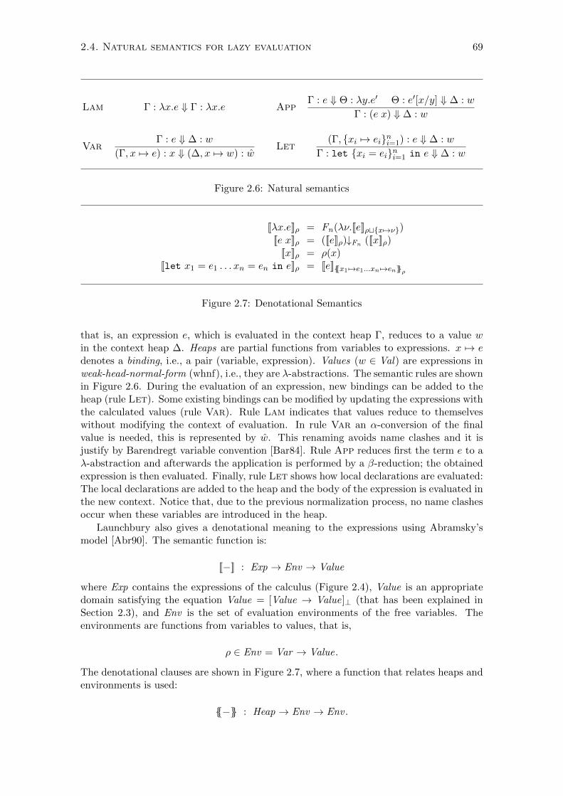
2.4. Natural semantics for lazy evaluation 69
Lam Γ : λx.e ⇓ Γ : λx.e AppΓ : e ⇓ Θ : λy.e′ Θ : e′[x/y] ⇓ ∆ : w
Γ : (e x) ⇓ ∆ : w
VarΓ : e ⇓ ∆ : w
(Γ, x 7→ e) : x ⇓ (∆, x 7→ w) : wLet
(Γ, {xi 7→ ei}ni=1) : e ⇓ ∆ : w
Γ : let {xi = ei}ni=1 in e ⇓ ∆ : w
Figure 2.6: Natural semantics
[[λx.e]]ρ = Fn(λν.[[e]]ρt{x 7→ν})
[[e x]]ρ = ([[e]]ρ)↓Fn ([[x]]ρ)[[x]]ρ = ρ(x)
[[let x1 = e1 . . . xn = en in e]]ρ = [[e]]{{x1 7→e1...xn 7→en}}ρ
Figure 2.7: Denotational Semantics
that is, an expression e, which is evaluated in the context heap Γ, reduces to a value win the context heap ∆. Heaps are partial functions from variables to expressions. x 7→ edenotes a binding, i.e., a pair (variable, expression). Values (w ∈ Val) are expressions inweak-head-normal-form (whnf), i.e., they are λ-abstractions. The semantic rules are shownin Figure 2.6. During the evaluation of an expression, new bindings can be added to theheap (rule Let). Some existing bindings can be modified by updating the expressions withthe calculated values (rule Var). Rule Lam indicates that values reduce to themselveswithout modifying the context of evaluation. In rule Var an α-conversion of the finalvalue is needed, this is represented by w. This renaming avoids name clashes and it isjustify by Barendregt variable convention [Bar84]. Rule App reduces first the term e to aλ-abstraction and afterwards the application is performed by a β-reduction; the obtainedexpression is then evaluated. Finally, rule Let shows how local declarations are evaluated:The local declarations are added to the heap and the body of the expression is evaluated inthe new context. Notice that, due to the previous normalization process, no name clashesoccur when these variables are introduced in the heap.
Launchbury also gives a denotational meaning to the expressions using Abramsky’smodel [Abr90]. The semantic function is:
[[−]] : Exp → Env → Value
where Exp contains the expressions of the calculus (Figure 2.4), Value is an appropriatedomain satisfying the equation Value = [Value → Value]⊥ (that has been explained inSection 2.3), and Env is the set of evaluation environments of the free variables. Theenvironments are functions from variables to values, that is,
ρ ∈ Env = Var → Value.
The denotational clauses are shown in Figure 2.7, where a function that relates heaps andenvironments is used:
{{−}} : Heap → Env → Env .
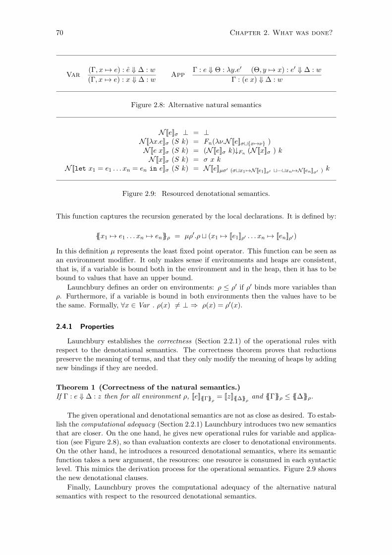
70 Chapter 2. What was done?
Var(Γ, x 7→ e) : e ⇓ ∆ : w
(Γ, x 7→ e) : x ⇓ ∆ : wApp
Γ : e ⇓ Θ : λy.e′ (Θ, y 7→ x) : e′ ⇓ ∆ : w
Γ : (e x) ⇓ ∆ : w
Figure 2.8: Alternative natural semantics
N [[e]]σ ⊥ = ⊥N [[λx.e]]σ (S k) = Fn(λν.N [[e]]σt{x 7→ν} )
N [[e x]]σ (S k) = (N [[e]]σ k)↓Fn (N [[x]]σ ) kN [[x]]σ (S k) = σ x k
N [[let x1 = e1 . . . xn = en in e]]σ (S k) = N [[e]]µσ′ (σtx1 7→N [[e1]]σ′ t···txn 7→N [[en]]σ′ ) k
Figure 2.9: Resourced denotational semantics.
This function captures the recursion generated by the local declarations. It is defined by:
{{x1 7→ e1 . . . xn 7→ en}}ρ = µρ′.ρ t (x1 7→ [[e1]]ρ′ . . . xn 7→ [[en]]ρ′)
In this definition µ represents the least fixed point operator. This function can be seen asan environment modifier. It only makes sense if environments and heaps are consistent,that is, if a variable is bound both in the environment and in the heap, then it has to bebound to values that have an upper bound.
Launchbury defines an order on environments: ρ ≤ ρ′ if ρ′ binds more variables thanρ. Furthermore, if a variable is bound in both environments then the values have to bethe same. Formally, ∀x ∈ Var . ρ(x) 6= ⊥ ⇒ ρ(x) = ρ′(x).
2.4.1 Properties
Launchbury establishes the correctness (Section 2.2.1) of the operational rules withrespect to the denotational semantics. The correctness theorem proves that reductionspreserve the meaning of terms, and that they only modify the meaning of heaps by addingnew bindings if they are needed.
Theorem 1 (Correctness of the natural semantics.)If Γ : e ⇓ ∆ : z then for all environment ρ, [[e]]{{Γ}}ρ = [[z]]{{∆}}ρ and {{Γ}}ρ ≤ {{∆}}ρ.
The given operational and denotational semantics are not as close as desired. To estab-lish the computational adequacy (Section 2.2.1) Launchbury introduces two new semanticsthat are closer. On the one hand, he gives new operational rules for variable and applica-tion (see Figure 2.8), so than evaluation contexts are closer to denotational environments.On the other hand, he introduces a resourced denotational semantics, where its semanticfunction takes a new argument, the resources: one resource is consumed in each syntacticlevel. This mimics the derivation process for the operational semantics. Figure 2.9 showsthe new denotational clauses.
Finally, Launchbury proves the computational adequacy of the alternative naturalsemantics with respect to the resourced denotational semantics.
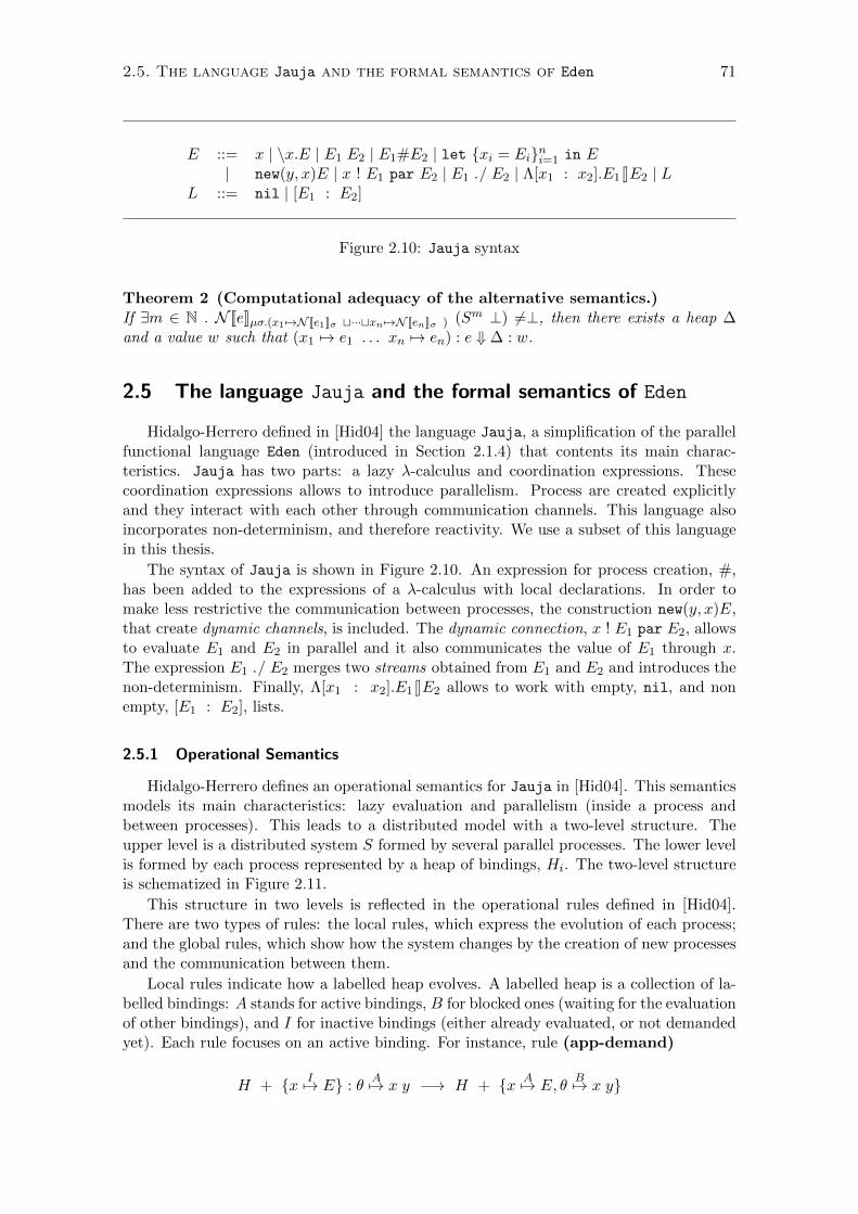
2.5. The language Jauja and the formal semantics of Eden 71
E ::= x | \x.E | E1 E2 | E1#E2 | let {xi = Ei}ni=1 in E| new(y, x)E | x ! E1 par E2 | E1 ./ E2 | Λ[x1 : x2].E1dcE2 | L
L ::= nil | [E1 : E2]
Figure 2.10: Jauja syntax
Theorem 2 (Computational adequacy of the alternative semantics.)If ∃m ∈ N . N [[e]]µσ.(x1 7→N [[e1]]σ t···txn 7→N [[en]]σ ) (Sm ⊥) 6=⊥, then there exists a heap ∆and a value w such that (x1 7→ e1 . . . xn 7→ en) : e ⇓ ∆ : w.
2.5 The language Jauja and the formal semantics of Eden
Hidalgo-Herrero defined in [Hid04] the language Jauja, a simplification of the parallelfunctional language Eden (introduced in Section 2.1.4) that contents its main charac-teristics. Jauja has two parts: a lazy λ-calculus and coordination expressions. Thesecoordination expressions allows to introduce parallelism. Process are created explicitlyand they interact with each other through communication channels. This language alsoincorporates non-determinism, and therefore reactivity. We use a subset of this languagein this thesis.
The syntax of Jauja is shown in Figure 2.10. An expression for process creation, #,has been added to the expressions of a λ-calculus with local declarations. In order tomake less restrictive the communication between processes, the construction new(y, x)E,that create dynamic channels, is included. The dynamic connection, x ! E1 par E2, allowsto evaluate E1 and E2 in parallel and it also communicates the value of E1 through x.The expression E1 ./ E2 merges two streams obtained from E1 and E2 and introduces thenon-determinism. Finally, Λ[x1 : x2].E1dcE2 allows to work with empty, nil, and nonempty, [E1 : E2], lists.
2.5.1 Operational Semantics
Hidalgo-Herrero defines an operational semantics for Jauja in [Hid04]. This semanticsmodels its main characteristics: lazy evaluation and parallelism (inside a process andbetween processes). This leads to a distributed model with a two-level structure. Theupper level is a distributed system S formed by several parallel processes. The lower levelis formed by each process represented by a heap of bindings, Hi. The two-level structureis schematized in Figure 2.11.
This structure in two levels is reflected in the operational rules defined in [Hid04].There are two types of rules: the local rules, which express the evolution of each process;and the global rules, which show how the system changes by the creation of new processesand the communication between them.
Local rules indicate how a labelled heap evolves. A labelled heap is a collection of la-belled bindings: A stands for active bindings, B for blocked ones (waiting for the evaluationof other bindings), and I for inactive bindings (either already evaluated, or not demandedyet). Each rule focuses on an active binding. For instance, rule (app-demand)
H + {x I7→ E} : θA7→ x y −→ H + {x A7→ E, θ
B7→ x y}
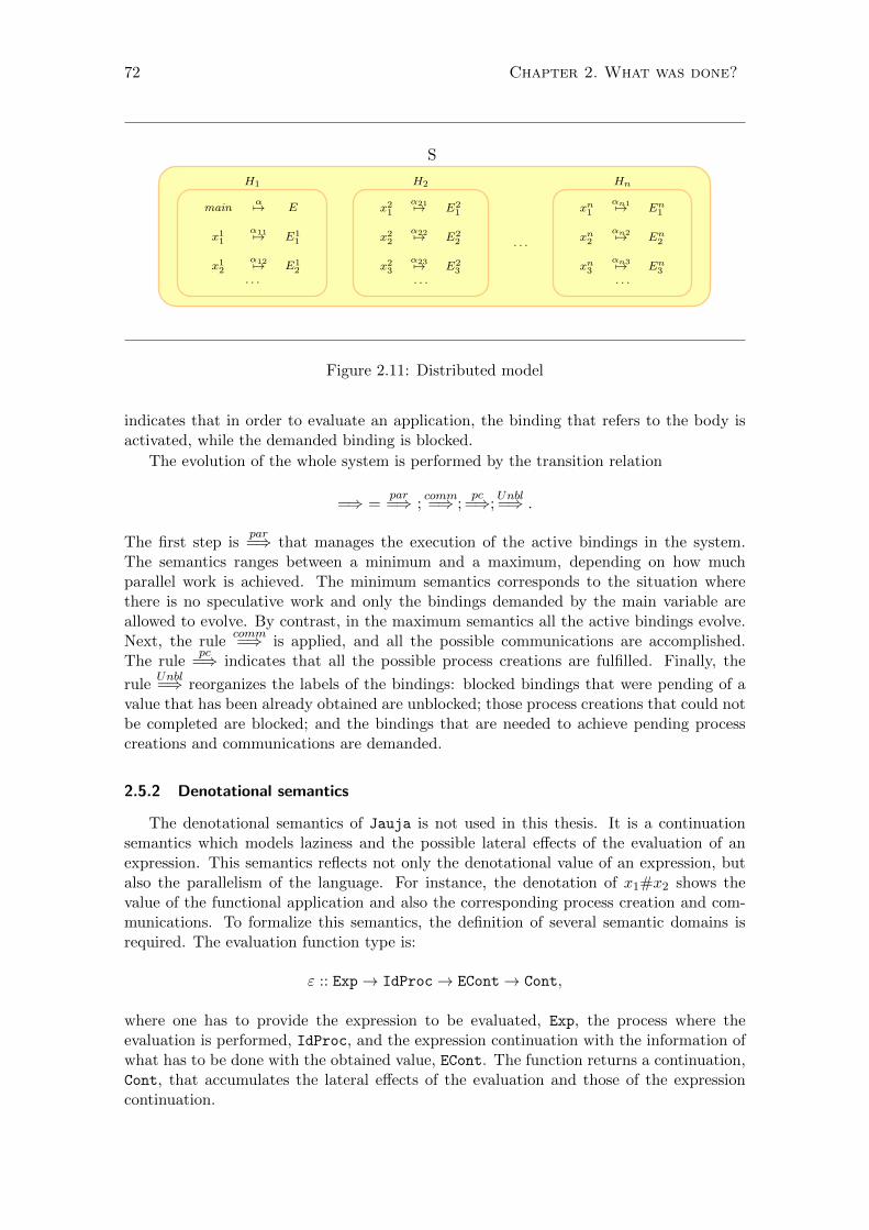
72 Chapter 2. What was done?
S
H1 H2 Hn
mainα7→ E
x11
α117→ E11
x12
α127→ E12
. . .
x21
α217→ E21
x22
α227→ E22
x23
α237→ E23
. . .
. . .
xn1
αn17→ En
1
xn2
αn27→ En
2
xn3
αn37→ En
3
. . .
Figure 2.11: Distributed model
indicates that in order to evaluate an application, the binding that refers to the body isactivated, while the demanded binding is blocked.
The evolution of the whole system is performed by the transition relation
=⇒ =par=⇒ ;
comm=⇒ ;
pc=⇒;
Unbl=⇒ .
The first step ispar=⇒ that manages the execution of the active bindings in the system.
The semantics ranges between a minimum and a maximum, depending on how muchparallel work is achieved. The minimum semantics corresponds to the situation wherethere is no speculative work and only the bindings demanded by the main variable areallowed to evolve. By contrast, in the maximum semantics all the active bindings evolve.Next, the rule
comm=⇒ is applied, and all the possible communications are accomplished.
The rulepc
=⇒ indicates that all the possible process creations are fulfilled. Finally, the
ruleUnbl=⇒ reorganizes the labels of the bindings: blocked bindings that were pending of a
value that has been already obtained are unblocked; those process creations that could notbe completed are blocked; and the bindings that are needed to achieve pending processcreations and communications are demanded.
2.5.2 Denotational semantics
The denotational semantics of Jauja is not used in this thesis. It is a continuationsemantics which models laziness and the possible lateral effects of the evaluation of anexpression. This semantics reflects not only the denotational value of an expression, butalso the parallelism of the language. For instance, the denotation of x1#x2 shows thevalue of the functional application and also the corresponding process creation and com-munications. To formalize this semantics, the definition of several semantic domains isrequired. The evaluation function type is:
ε :: Exp→ IdProc→ ECont→ Cont,
where one has to provide the expression to be evaluated, Exp, the process where theevaluation is performed, IdProc, and the expression continuation with the information ofwhat has to be done with the obtained value, ECont. The function returns a continuation,Cont, that accumulates the lateral effects of the evaluation and those of the expressioncontinuation.
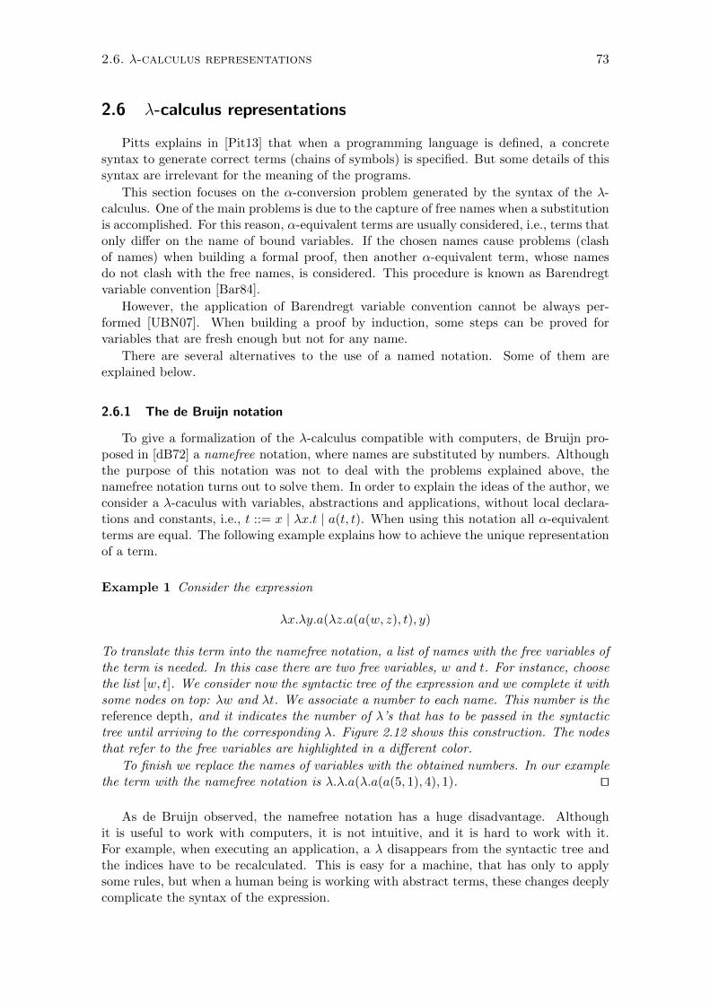
2.6. λ-calculus representations 73
2.6 λ-calculus representations
Pitts explains in [Pit13] that when a programming language is defined, a concretesyntax to generate correct terms (chains of symbols) is specified. But some details of thissyntax are irrelevant for the meaning of the programs.
This section focuses on the α-conversion problem generated by the syntax of the λ-calculus. One of the main problems is due to the capture of free names when a substitutionis accomplished. For this reason, α-equivalent terms are usually considered, i.e., terms thatonly differ on the name of bound variables. If the chosen names cause problems (clashof names) when building a formal proof, then another α-equivalent term, whose namesdo not clash with the free names, is considered. This procedure is known as Barendregtvariable convention [Bar84].
However, the application of Barendregt variable convention cannot be always per-formed [UBN07]. When building a proof by induction, some steps can be proved forvariables that are fresh enough but not for any name.
There are several alternatives to the use of a named notation. Some of them areexplained below.
2.6.1 The de Bruijn notation
To give a formalization of the λ-calculus compatible with computers, de Bruijn pro-posed in [dB72] a namefree notation, where names are substituted by numbers. Althoughthe purpose of this notation was not to deal with the problems explained above, thenamefree notation turns out to solve them. In order to explain the ideas of the author, weconsider a λ-caculus with variables, abstractions and applications, without local declara-tions and constants, i.e., t ::= x | λx.t | a(t, t). When using this notation all α-equivalentterms are equal. The following example explains how to achieve the unique representationof a term.
Example 1 Consider the expression
λx.λy.a(λz.a(a(w, z), t), y)
To translate this term into the namefree notation, a list of names with the free variables ofthe term is needed. In this case there are two free variables, w and t. For instance, choosethe list [w, t]. We consider now the syntactic tree of the expression and we complete it withsome nodes on top: λw and λt. We associate a number to each name. This number is thereference depth, and it indicates the number of λ’s that has to be passed in the syntactictree until arriving to the corresponding λ. Figure 2.12 shows this construction. The nodesthat refer to the free variables are highlighted in a different color.
To finish we replace the names of variables with the obtained numbers. In our examplethe term with the namefree notation is λ.λ.a(λ.a(a(5, 1), 4), 1). ut
As de Bruijn observed, the namefree notation has a huge disadvantage. Althoughit is useful to work with computers, it is not intuitive, and it is hard to work with it.For example, when executing an application, a λ disappears from the syntactic tree andthe indices have to be recalculated. This is easy for a machine, that has only to applysome rules, but when a human being is working with abstract terms, these changes deeplycomplicate the syntax of the expression.
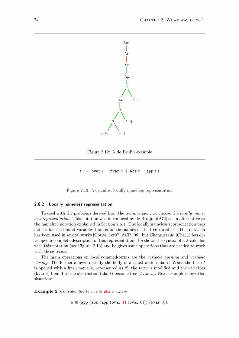
74 Chapter 2. What was done?
w z
a t
a
λz y
a
λy
λx
λt
λw
5 1
4
1
Figure 2.12: A de Bruijn example
t := bvar i | fvar x | abs t | app t t
Figure 2.13: λ-calculus, locally nameless representation
2.6.2 Locally nameless representation
To deal with the problems derived from the α-conversion, we choose the locally name-less representation. This notation was introduced by de Bruijn [dB72] as an alternative tothe namefree notation explained in Section 2.6.1. The locally nameless representation usesindices for the bound variables but retain the names of the free variables. This notationhas been used in several works [Gor94, Ler07, ACP+08], but Chargueraud [Cha11] has de-veloped a complete description of this representation. He shows the syntax of a λ-calculuswith this notation (see Figure 2.13) and he gives some operations that are needed to workwith these terms.
The main operations on locally-named-terms are the variable opening and variableclosing. The former allows to study the body of an abstraction abs t. When the term tis opened with a fresh name x, represented as tx, the term is modified and the variables(bvar i) bound to the abstraction (abs t) become free (fvar x). Next example shows thissituation:
Example 2 Consider the term t ≡ abs u where
u ≡ (app (abs (app (bvar 1) (bvar 0))) (bvar 0)).
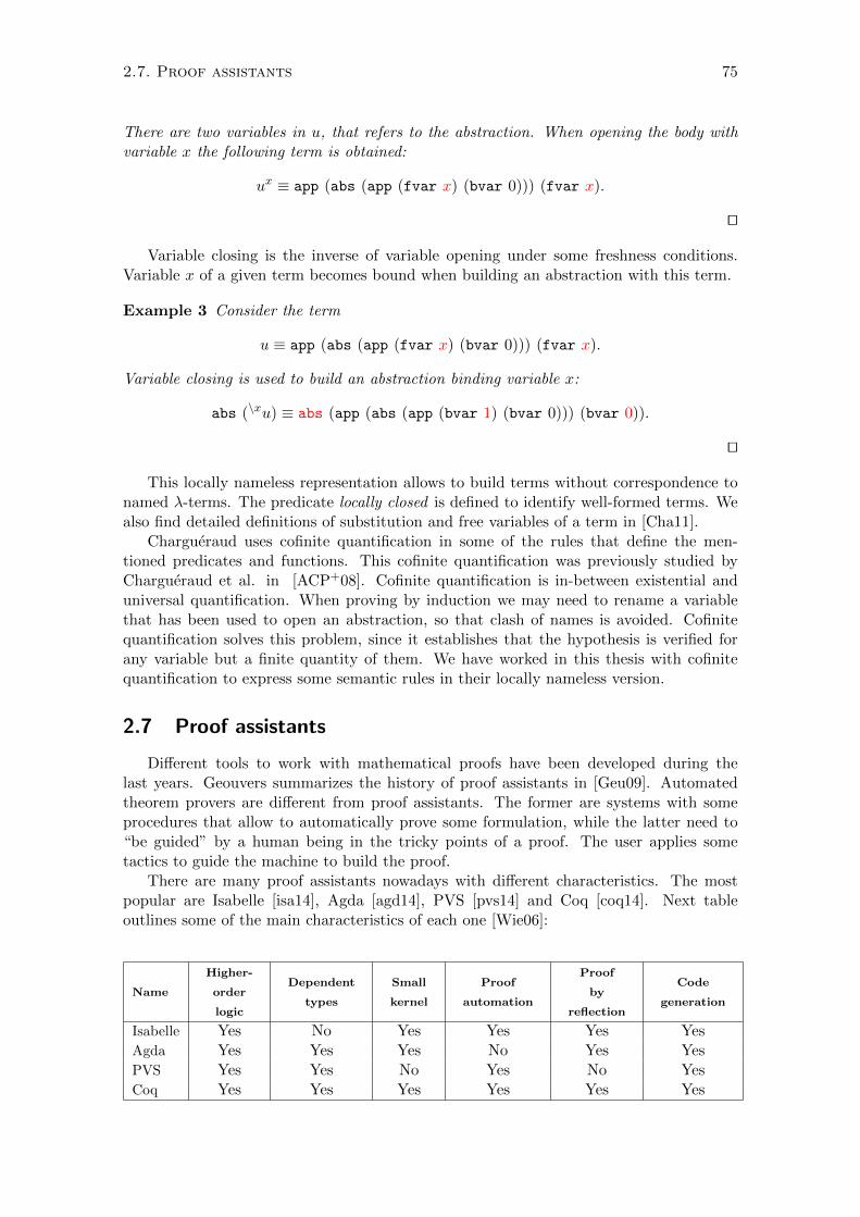
2.7. Proof assistants 75
There are two variables in u, that refers to the abstraction. When opening the body withvariable x the following term is obtained:
ux ≡ app (abs (app (fvar x) (bvar 0))) (fvar x).
ut
Variable closing is the inverse of variable opening under some freshness conditions.Variable x of a given term becomes bound when building an abstraction with this term.
Example 3 Consider the term
u ≡ app (abs (app (fvar x) (bvar 0))) (fvar x).
Variable closing is used to build an abstraction binding variable x:
abs (\xu) ≡ abs (app (abs (app (bvar 1) (bvar 0))) (bvar 0)).
ut
This locally nameless representation allows to build terms without correspondence tonamed λ-terms. The predicate locally closed is defined to identify well-formed terms. Wealso find detailed definitions of substitution and free variables of a term in [Cha11].
Chargueraud uses cofinite quantification in some of the rules that define the men-tioned predicates and functions. This cofinite quantification was previously studied byChargueraud et al. in [ACP+08]. Cofinite quantification is in-between existential anduniversal quantification. When proving by induction we may need to rename a variablethat has been used to open an abstraction, so that clash of names is avoided. Cofinitequantification solves this problem, since it establishes that the hypothesis is verified forany variable but a finite quantity of them. We have worked in this thesis with cofinitequantification to express some semantic rules in their locally nameless version.
2.7 Proof assistants
Different tools to work with mathematical proofs have been developed during thelast years. Geouvers summarizes the history of proof assistants in [Geu09]. Automatedtheorem provers are different from proof assistants. The former are systems with someprocedures that allow to automatically prove some formulation, while the latter need to“be guided” by a human being in the tricky points of a proof. The user applies sometactics to guide the machine to build the proof.
There are many proof assistants nowadays with different characteristics. The mostpopular are Isabelle [isa14], Agda [agd14], PVS [pvs14] and Coq [coq14]. Next tableoutlines some of the main characteristics of each one [Wie06]:
Name
Higher-
order
logic
Dependent
types
Small
kernel
Proof
automation
Proof
by
reflection
Code
generation
Isabelle Yes No Yes Yes Yes YesAgda Yes Yes Yes No Yes YesPVS Yes Yes No Yes No YesCoq Yes Yes Yes Yes Yes Yes
76 Chapter 2. What was done?
Only the rules that form the kernel of a proof assistant must be proven to be correct;the others are built from them. For this reason it is important to have a small kernel.
We have used Coq in thesis to extend some definitions and results implemented byChargueraud in [Cha11]. They refer to the locally nameless representation given in Sec-tion 2.6.2.
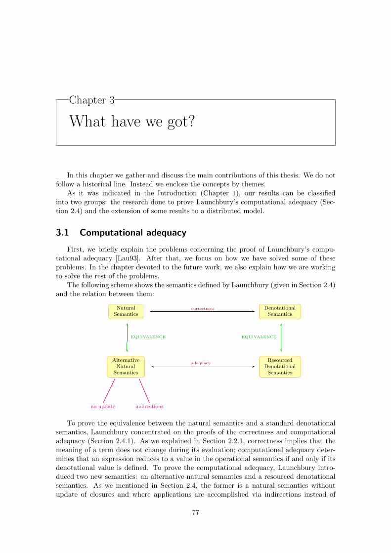
Chapter 3
What have we got?
In this chapter we gather and discuss the main contributions of this thesis. We do notfollow a historical line. Instead we enclose the concepts by themes.
As it was indicated in the Introduction (Chapter 1), our results can be classifiedinto two groups: the research done to prove Launchbury’s computational adequacy (Sec-tion 2.4) and the extension of some results to a distributed model.
3.1 Computational adequacy
First, we briefly explain the problems concerning the proof of Launchbury’s compu-tational adequacy [Lau93]. After that, we focus on how we have solved some of theseproblems. In the chapter devoted to the future work, we also explain how we are workingto solve the rest of the problems.
The following scheme shows the semantics defined by Launchbury (given in Section 2.4)and the relation between them:
NaturalSemantics
DenotationalSemantics
AlternativeNatural
Semantics
ResourcedDenotationalSemantics
correctness
adequacy
EQUIVALENCE EQUIVALENCE
no update indirections
To prove the equivalence between the natural semantics and a standard denotationalsemantics, Launchbury concentrated on the proofs of the correctness and computationaladequacy (Section 2.4.1). As we explained in Section 2.2.1, correctness implies that themeaning of a term does not change during its evaluation; computational adequacy deter-mines that an expression reduces to a value in the operational semantics if and only if itsdenotational value is defined. To prove the computational adequacy, Launchbury intro-duced two new semantics: an alternative natural semantics and a resourced denotationalsemantics. As we mentioned in Section 2.4, the former is a natural semantics withoutupdate of closures and where applications are accomplished via indirections instead of
77
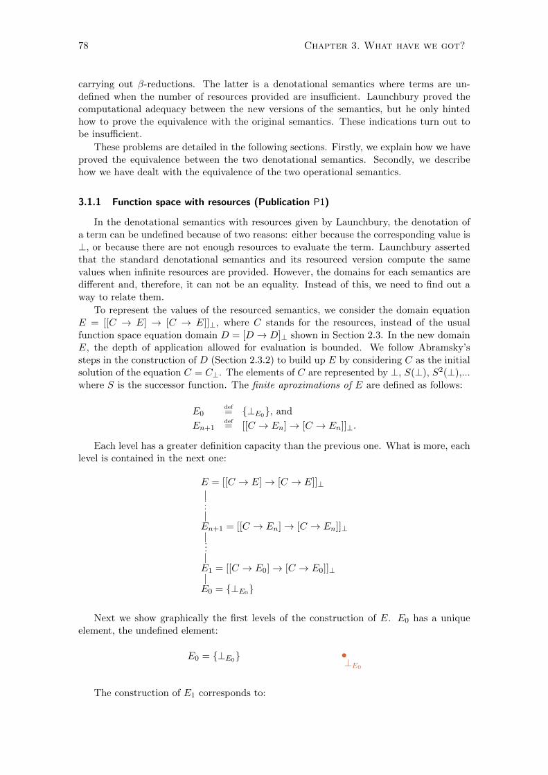
78 Chapter 3. What have we got?
carrying out β-reductions. The latter is a denotational semantics where terms are un-defined when the number of resources provided are insufficient. Launchbury proved thecomputational adequacy between the new versions of the semantics, but he only hintedhow to prove the equivalence with the original semantics. These indications turn out tobe insufficient.
These problems are detailed in the following sections. Firstly, we explain how we haveproved the equivalence between the two denotational semantics. Secondly, we describehow we have dealt with the equivalence of the two operational semantics.
3.1.1 Function space with resources (Publication P1)
In the denotational semantics with resources given by Launchbury, the denotation ofa term can be undefined because of two reasons: either because the corresponding value is⊥, or because there are not enough resources to evaluate the term. Launchbury assertedthat the standard denotational semantics and its resourced version compute the samevalues when infinite resources are provided. However, the domains for each semantics aredifferent and, therefore, it can not be an equality. Instead of this, we need to find out away to relate them.
To represent the values of the resourced semantics, we consider the domain equationE = [[C → E] → [C → E]]⊥, where C stands for the resources, instead of the usualfunction space equation domain D = [D → D]⊥ shown in Section 2.3. In the new domainE, the depth of application allowed for evaluation is bounded. We follow Abramsky’ssteps in the construction of D (Section 2.3.2) to build up E by considering C as the initialsolution of the equation C = C⊥. The elements of C are represented by ⊥, S(⊥), S2(⊥),...where S is the successor function. The finite aproximations of E are defined as follows:
E0def= {⊥E0}, and
En+1def= [[C → En]→ [C → En]]⊥.
Each level has a greater definition capacity than the previous one. What is more, eachlevel is contained in the next one:
E0 = {⊥E0}
|E1 = [[C → E0] → [C → E0]]⊥|
...|En+1 = [[C → En] → [C → En]]⊥|
..
.
|
E = [[C → E] → [C → E]]⊥
Next we show graphically the first levels of the construction of E. E0 has a uniqueelement, the undefined element:
E0 = {⊥E0}
⊥E0
The construction of E1 corresponds to:
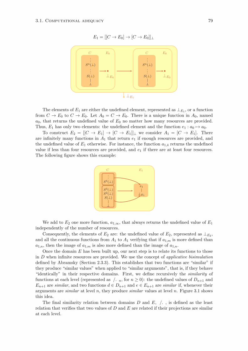
3.1. Computational adequacy 79
E1 = [[C → E0] → [C → E0]]⊥
C E0
.
.
.Sn(⊥)
.
.
.S(⊥)
|⊥
b
C E0
.
.
.Sn(⊥)
.
.
.S(⊥)
|⊥
b
b ⊥E1
⊥E0⊥E0
The elements of E1 are either the undefined element, represented as ⊥E1 , or a functionfrom C → E0 to C → E0. Let A0 = C → E0. There is a unique function in A0, nameda0, that returns the undefined value of E0 no matter how many resources are provided.Thus, E1 has only two elements: the undefined element and the function e1 : a0 7→ a0.
To construct E2 = [[C → E1] → [C → E1]]⊥ we consider A1 = [C → E1]. Thereare infinitely many functions in A1 that return e1 if enough resources are provided, andthe undefined value of E1 otherwise. For instance, the function a1,4 returns the undefinedvalue if less than four resources are provided, and e1 if there are at least four resources.The following figure shows this example:
C E1
.
.
.S4(⊥)
S3(⊥)S2(⊥)S(⊥)
|⊥
e1
|⊥E1
We add to E2 one more function, a1,∞, that always returns the undefined value of E1
independently of the number of resources.
Consequently, the elements of E2 are: the undefined value of E2, represented as ⊥E2 ,and all the continuous functions from A1 to A1 verifying that if a1,m is more defined thana1,n, then the image of a1,m is also more defined than the image of a1,n.
Once the domain E has been built up, our next step is to relate its functions to thosein D when infinite resources are provided. We use the concept of applicative bisimulationdefined by Abramsky (Section 2.3.3). This establishes that two functions are “similar” ifthey produce “similar values” when applied to “similar arguments”, that is, if they behave“identically” in their respective domains. First, we define recursively the similarity offunctions at each level (represented as /. n, for n ≥ 0): the undefined values of Dn+1 andEn+1 are similar, and two functions d ∈ Dn+1 and e ∈ En+1 are similar if, whenever theirarguments are similar at level n, they produce similar values at level n. Figure 3.1 showsthis idea.
The final similarity relation between domains D and E, /. , is defined as the leastrelation that verifies that two values of D and E are related if their projections are similarat each level.

80 Chapter 3. What have we got?
d′ a′(S∞)n
⊳⊲n
+
d(d′) e(a′)(S∞)n
⊳⊲n
⇓
d en+ 1
⊥Dn+1⊥En+1
⊳⊲n+1
Figure 3.1: Intuition of similarity
There is an alternative characterization of the relation /. that asserts that two valuesof D and E are related either if both are undefined, or if similar values are obtained whenapplied to similar arguments. This statement is formally written in the next proposition:
Proposition 1Let d ∈ D, e ∈ E. d /. e if and only if either:
(d =⊥D ∧ e =⊥E), or
(d 6=⊥D ∧ e 6=⊥E) ∧ ∀d′ ∈ D.∀a′ ∈ [C → E].d′ /. a′(S∞)⇒ d(d′) /. e(a′)(S∞).
Finally we apply this result to prove the equivalence of the two denotational seman-tics proposed by Launchbury. For this purpose we extend the concept of similarity toenvironments. An environment ρ of the standard denotational semantics is similar to anenvironment σ of the resourced denotational semantics when infinite resources are pro-vided, if the values associated to each variable in their respective domains are similar. Wecan prove now the following theorem:
Theorem 3 (Equivalence of denotational semantics.)If e ∈ Exp and ρ /. σ, then [[e]]ρ /. N [[e]]σ (S∞).
Summary of results.
1. Construction of the initial solution of the domain equationE = [[C → E] → [C → E]]⊥, where C stands for the domain of resources.
2. Definition of the relation of similarity between the values of the domain E
and the values of the standard function space D = [D → D]⊥.3. Application of the previous result to prove the equivalence between the
denotational standard semantics and the resourced denotational semantics forthe lazy λ-calculus.
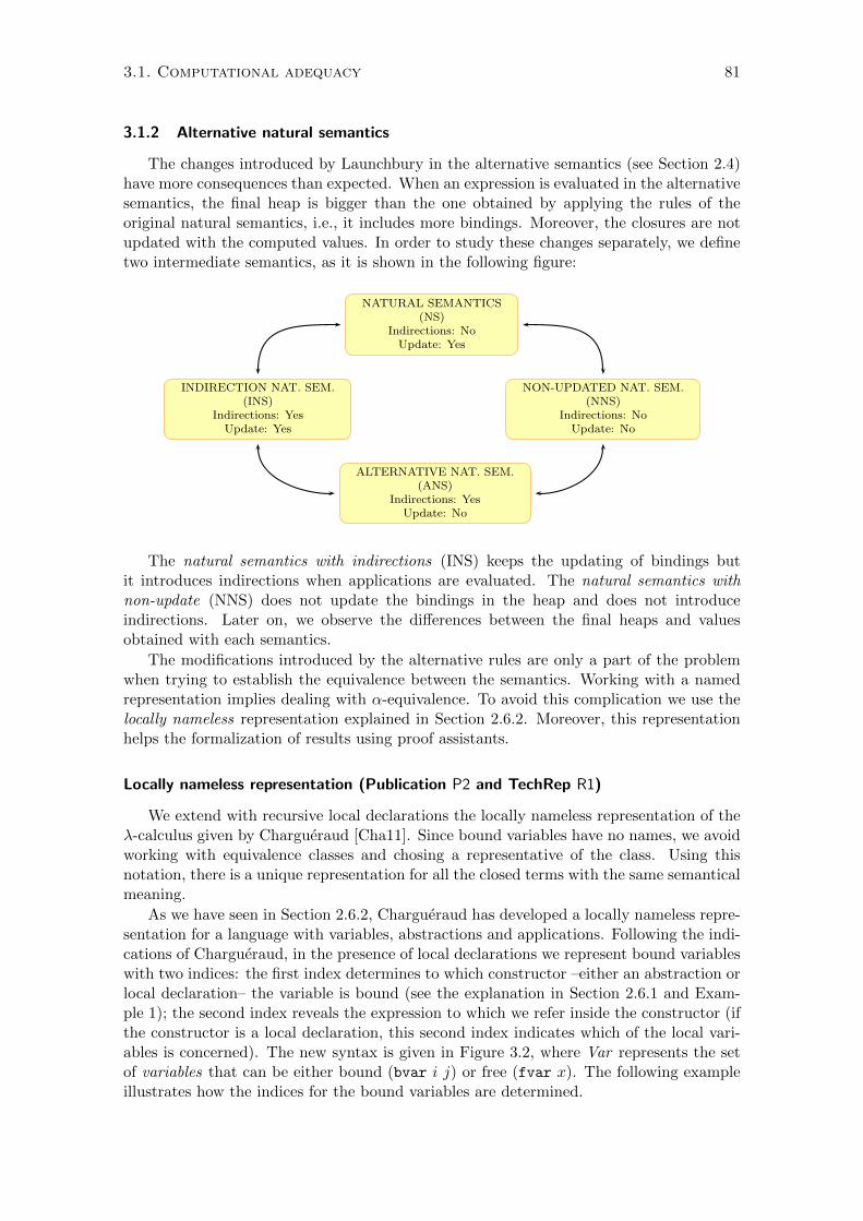
3.1. Computational adequacy 81
3.1.2 Alternative natural semantics
The changes introduced by Launchbury in the alternative semantics (see Section 2.4)have more consequences than expected. When an expression is evaluated in the alternativesemantics, the final heap is bigger than the one obtained by applying the rules of theoriginal natural semantics, i.e., it includes more bindings. Moreover, the closures are notupdated with the computed values. In order to study these changes separately, we definetwo intermediate semantics, as it is shown in the following figure:
NATURAL SEMANTICS(NS)
Indirections: NoUpdate: Yes
INDIRECTION NAT. SEM.(INS)
Indirections: YesUpdate: Yes
NON-UPDATED NAT. SEM.(NNS)
Indirections: NoUpdate: No
ALTERNATIVE NAT. SEM.(ANS)
Indirections: YesUpdate: No
The natural semantics with indirections (INS) keeps the updating of bindings butit introduces indirections when applications are evaluated. The natural semantics withnon-update (NNS) does not update the bindings in the heap and does not introduceindirections. Later on, we observe the differences between the final heaps and valuesobtained with each semantics.
The modifications introduced by the alternative rules are only a part of the problemwhen trying to establish the equivalence between the semantics. Working with a namedrepresentation implies dealing with α-equivalence. To avoid this complication we use thelocally nameless representation explained in Section 2.6.2. Moreover, this representationhelps the formalization of results using proof assistants.
Locally nameless representation (Publication P2 and TechRep R1)
We extend with recursive local declarations the locally nameless representation of theλ-calculus given by Chargueraud [Cha11]. Since bound variables have no names, we avoidworking with equivalence classes and chosing a representative of the class. Using thisnotation, there is a unique representation for all the closed terms with the same semanticalmeaning.
As we have seen in Section 2.6.2, Chargueraud has developed a locally nameless repre-sentation for a language with variables, abstractions and applications. Following the indi-cations of Chargueraud, in the presence of local declarations we represent bound variableswith two indices: the first index determines to which constructor –either an abstraction orlocal declaration– the variable is bound (see the explanation in Section 2.6.1 and Exam-ple 1); the second index reveals the expression to which we refer inside the constructor (ifthe constructor is a local declaration, this second index indicates which of the local vari-ables is concerned). The new syntax is given in Figure 3.2, where Var represents the setof variables that can be either bound (bvar i j) or free (fvar x). The following exampleillustrates how the indices for the bound variables are determined.

82 Chapter 3. What have we got?
x ∈ Id i, j ∈ Nv ∈ Var ::= bvar i j | fvar xt ∈ LNExp ::= v | abs t | app t v | let {ti}ni=1 in t
Figure 3.2: Locally nameless syntax
Example 4 The expression e is a λ-abstraction whose body is a let-expression with twolocal declarations.
e ≡ λz.let x1 = λy1.y1,x2 = λy2.y2,
in (z x2)
This expression is represented in the locally nameless notation by t:
t ≡ abs (let abs (bvar 0 0), abs (bvar 0 0) in app (bvar 1 0) (bvar 0 1)).
The expression bounded to x1 appears in green, the one bounded to x2 in red, and the mainterm in blue.
Let us see the syntactic tree to clarify how the indices point to the constructors:
abs
let
abs abs app
bvar bvar bvar bvar
0 0 0 0 1 0 0 1
Notice that the second index of the variable that points to the let expression is red.This indicates that it refers to the local declaration that appears with that color inside thelet constructor. ut
Although Chargueraud suggests how the language should be extended with local dec-larations, this study is not fully developed. The opening of a term and the rules for localclosure are explained, but the rest of operators and functions over terms are not definedin [Cha11]. We have extended the following functions: The closure of terms, the predicateof local closure at level k, the free variables of a term, the substitution and the conceptof freshness. We have also extended some results such as the one which asserts that theopening and closing of a term are inverse functions under some conditions.
Once we have established the operators and functions needed to work with the locallynameless representation, we have reformulated Launchbury’s semantic rules (Figure 2.4in Section 2.4). First we have redefined the heaps as sets of pairs of the form (fvar x, t),and we have readjusted all the concepts related with them: domain of a heap, namesthat appear in a heap, well-formed heaps and substitutions on heaps. Moreover, we haveproved some useful properties derived from this notation.

3.1. Computational adequacy 83
LNLet∀x|t| /∈ L ⊆ Id (Γ, x 7→ t
x) : tx ⇓ (x++z 7→ ux) : wx {y|t| /∈ L ⊆ Id}
Γ : let t in t ⇓ (y ++z 7→ uy) : wy
Figure 3.3: Variable local declaration (locally nameless representation)
We have already explained in Section 2.6.2 that the locally nameless representationallows the formation of incorrect terms, in the sense that they do not correspond to anyterm in the λ-calculus. Therefore, we have added some premises to the semantic rules toensure that they are restricted to well-formed heaps and correct terms, i.e., locally closedterms.
Here we just highlight the new version of the rule for local declarations, that is, theLNLet rule shown in Figure 3.3. Tuples are represented as t, if they refer to terms, or x,if they refer to variables. To evaluate the expression let t in t, the local declarations tare added to the heap. Since we are using the locally nameless representation, the namesof the local variables are not explicit and we need to choose a list of fresh names x. Thesenames are used to open the local terms and the body of the expression. The evaluationof tx produces a final heap and value that are dependent on the chosen names. In thefinal heap these names, x, are explicitly shown, and the rest of names are represented byz. We use cofinite quantification in the rule LNLet. As it is explained in [Cha11], theadvantage of this quantification is that the side-conditions concerning the freshness of xare not detailed. These conditions are implicit in the set L. This set contains all thenames that must be avoided during the reduction, in particular those that appear in otherparts of the derivation. Our cofinite rule is different from the ones described in [Cha11],because the chosen names appear also in the conclusion. As a result, we have that thenew names x can be replaced by any list of names y that are not in L.
After translating the semantic rules of the natural semantics and its alternative versioninto the locally nameless notation1, we have proved some properties, for instance:
Regularity ensures that the judgements produced by these reduction systems yield onlywell-formed heaps and locally closed terms;
Renaming indicates that the evaluation of a term is independent of the fresh nameschosen during the derivation;
Introduction establishes a correct existential rule for each cofinite rule.
Summary of results.
1. Locally nameless representation of the λ-calculus extended with recursivelocal declarations.
2. Locally nameless representation of Launchbury’s natural semantic rules and itsalternative version.
3. Properties of the reduction systems (regularity, introduction and renaming).
1The translation of the alternative rules into the locally nameless notation do not appear in P2 but inP3, which is explained in next section. However, we have considered more convenient to refer them in thissection that is devoted to the locally nameless representation.

84 Chapter 3. What have we got?
An Indirection relation (Publication P3 and TechRep R2)
Once the semantic rules have been translated into the locally nameless representation,we can explore the equivalence between the non-updated semantics (NNS) and the alter-native semantics (ANS). We want to prove that the result obtained by both semanticswhen evaluating a term in a given context are the “same”. This equivalence is highlightedin the following diagram:
NATURAL SEMANTICS(NS)
Indirections: NoUpdate: Yes
INDIRECTION NAT. SEM.(INS)
Indirections: YesUpdate: Yes
NON-UPDATED NAT. SEM.(NNS)
Indirections: NoUpdate: No
ALTERNATIVE NAT. SEM.(ANS)
Indirections: YesUpdate: No
Both semantics use the same semantic rules except for the application rule. The NNSuses the LNApp rule, where the application is performed by a β-reduction, while the ANSapplies the ALNApp rule, where an indirection is introduced in the heap. Although thisdistinction seems to be irrelevant, the final heaps obtained in derivations are different.Those obtained by evaluating with the ANS are bigger than the ones obtained by usingthe rules of the NNS. Notice that an “extra” binding is introduced in the heap each timean application is performed. This binding is an indirection, i.e., a name bound to a name.Therefore, final heaps cannot be the same and we study the relation between them. Ourfirst idea was just to remove the indirections and check for the equality of the resultingheaps. However, this is insufficient, since some closures in the final heap could depend onthe removed bindings.
Next example shows this problem. ⇓N indicates a derivation for NNS is being applied,while ⇓A refers to ANS:
Example 5 Consider the following term:
t ≡ let abs (bvar 0 0) in app (abs s) (bvar 0 0)s ≡ let abs (bvar 0 0), app (bvar 0 0) (bvar 1 0) in abs (bvar 0 0)
If we evaluate t (in the context of an empty heap) we obtain abs (bvar 0 0) as final valuein both cases, but different final heaps are built:
{ } : t
⇓N
x0 7→ abs (bvar 0 0),x1 7→ abs (bvar 0 0),x2 7→ app (fvar x1) (fvar x0)
{ } : t
⇓A
x0 7→ abs (bvar 0 0),x1 7→ abs (bvar 0 0),x2 7→ app (fvar x1) (fvar y)y 7→ (fvar x0)
We observe that the final heap obtained by evaluating with the alternative semantics hasan extra binding; moreover, the term associated to the name x2 depends on it. ut
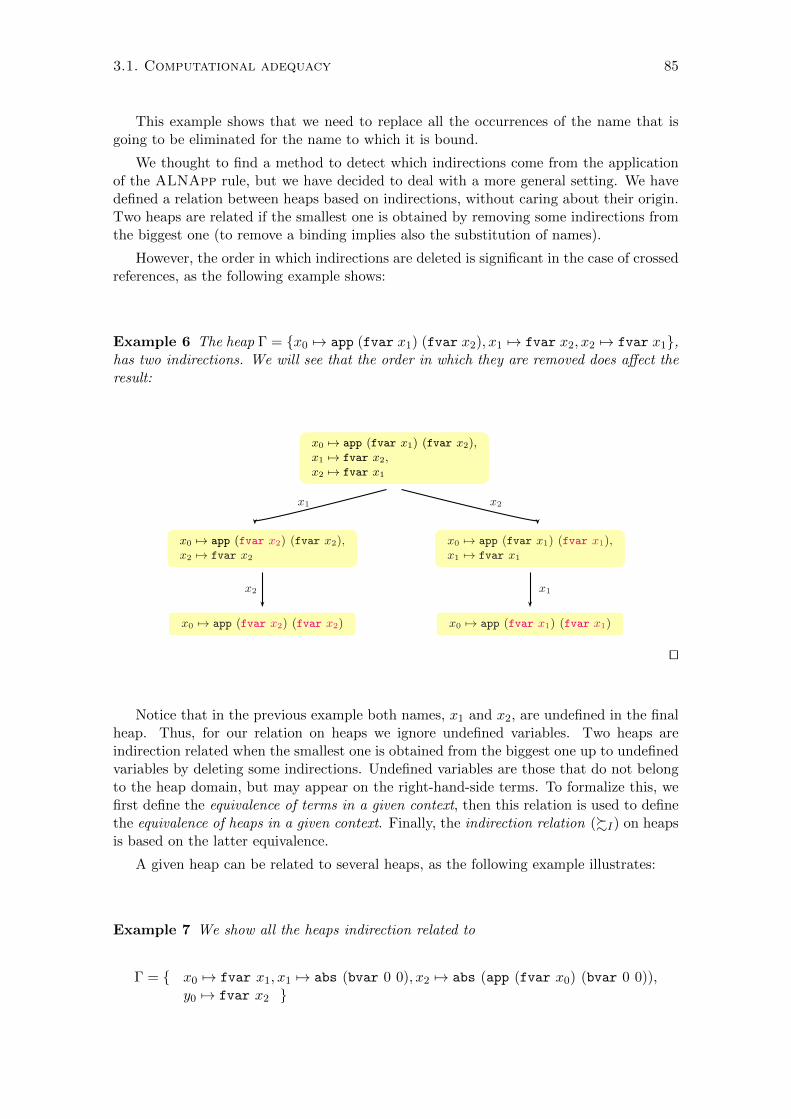
3.1. Computational adequacy 85
This example shows that we need to replace all the occurrences of the name that isgoing to be eliminated for the name to which it is bound.
We thought to find a method to detect which indirections come from the applicationof the ALNApp rule, but we have decided to deal with a more general setting. We havedefined a relation between heaps based on indirections, without caring about their origin.Two heaps are related if the smallest one is obtained by removing some indirections fromthe biggest one (to remove a binding implies also the substitution of names).
However, the order in which indirections are deleted is significant in the case of crossedreferences, as the following example shows:
Example 6 The heap Γ = {x0 7→ app (fvar x1) (fvar x2), x1 7→ fvar x2, x2 7→ fvar x1},has two indirections. We will see that the order in which they are removed does affect theresult:
x0 7→ app (fvar x1) (fvar x2),x1 7→ fvar x2,
x2 7→ fvar x1
x0 7→ app (fvar x2) (fvar x2),x2 7→ fvar x2
x0 7→ app (fvar x1) (fvar x1),x1 7→ fvar x1
x0 7→ app (fvar x2) (fvar x2) x0 7→ app (fvar x1) (fvar x1)
x1 x2
x2 x1
ut
Notice that in the previous example both names, x1 and x2, are undefined in the finalheap. Thus, for our relation on heaps we ignore undefined variables. Two heaps areindirection related when the smallest one is obtained from the biggest one up to undefinedvariables by deleting some indirections. Undefined variables are those that do not belongto the heap domain, but may appear on the right-hand-side terms. To formalize this, wefirst define the equivalence of terms in a given context, then this relation is used to definethe equivalence of heaps in a given context. Finally, the indirection relation (%I) on heapsis based on the latter equivalence.
A given heap can be related to several heaps, as the following example illustrates:
Example 7 We show all the heaps indirection related to
Γ = { x0 7→ fvar x1, x1 7→ abs (bvar 0 0), x2 7→ abs (app (fvar x0) (bvar 0 0)),y0 7→ fvar x2 }
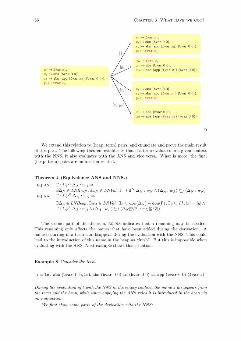
86 Chapter 3. What have we got?
x0 7→ fvar x1,
x1 7→ abs (bvar 0 0),x2 7→ abs (app (fvar x0) (bvar 0 0)),y0 7→ fvar x2
x0 7→ fvar x1,
x1 7→ abs (bvar 0 0),x2 7→ abs (app (fvar x0) (bvar 0 0)),y0 7→ fvar x2
x0 7→ fvar x1,
x1 7→ abs (bvar 0 0),x2 7→ abs (app (fvar x0) (bvar 0 0))
x1 7→ abs (bvar 0 0),x2 7→ abs (app (fvar x1) (bvar 0 0)),y0 7→ fvar x2
x1 7→ abs (bvar 0 0),x2 7→ abs (app (fvar x1) (bvar 0 0))
[ ]
[y0]
[x0]
[x0, y0]
ut
We extend this relation to (heap, term) pairs, and enunciate and prove the main resultof this part. The following theorem establishes that if a term evaluates in a given contextwith the NNS, it also evaluates with the ANS and vice versa. What is more, the final(heap, term) pairs are indirection related.
Theorem 4 (Equivalence ANS and NNS.)
eq an Γ : t ⇓A ∆A : wA ⇒∃∆N ∈ LNHeap . ∃wN ∈ LNVal .Γ : t ⇓N ∆N : wN ∧ (∆A : wA) %I (∆N : wN )
eq na Γ : t ⇓N ∆N : wN ⇒∃∆A ∈ LNHeap .∃wA ∈ LNVal . ∃x ⊆ dom(∆N )− dom(Γ) .∃y ⊆ Id . |x| = |y| ∧Γ : t ⇓A ∆A : wA ∧ (∆A : wA) %I (∆N [y/x] : wN [y/x])
The second part of the theorem, eq na indicates that a renaming may be needed.This renaming only affects the names that have been added during the derivation. Aname occurring in a term can disappear during the evaluation with the NNS. This couldlead to the introduction of this name in the heap as “fresh”. But this is impossible whenevaluating with the ANS. Next example shows this situation:
Example 8 Consider the term
t ≡ let abs (bvar 1 1), let abs (bvar 0 0) in (bvar 0 0) in app (bvar 0 0) (fvar z)
During the evaluation of t with the NNS in the empty context, the name z disappears fromthe term and the heap, while when applying the ANS rules it is introduced in the heap viaan indirection.
We first show some parts of the derivation with the NNS:

3.1. Computational adequacy 87
{ } : t{x0 7→ abs (fvar x1), x1 7→ let abs (bvar 0 0) in (bvar 0 0)} : app (fvar x0) (fvar z)
{x0 7→ abs (fvar x1), x1 7→ let abs (bvar 0 0) in (bvar 0 0)} : fvar x0{x0 7→ abs (fvar x1), x1 7→ let abs (bvar 0 0) in (bvar 0 0)} : abs fvar x1{x0 7→ abs (fvar x1), x1 7→ let abs (bvar 0 0) in (bvar 0 0)} : abs fvar x1
{x0 7→ abs (fvar x1), x1 7→ let abs (bvar 0 0) in (bvar 0 0)} : abs fvar x1
{x0 7→ abs (fvar x1), x1 7→ let abs (bvar 0 0) in (bvar 0 0)} : fvar x1{x0 7→ abs (fvar x1), x1 7→ let abs (bvar 0 0) in (bvar 0 0)} : let abs (bvar 0 0) in (bvar 0 0)...{x0 7→ abs (fvar x1), x1 7→ let abs (bvar 0 0) in (bvar 0 0),x2 7→ abs (bvar 0 0)
}: abs (bvar 0 0)
{x0 7→ abs (fvar x1), x1 7→ let abs (bvar 0 0) in (bvar 0 0),x2 7→ abs (bvar 0 0)
}: abs (bvar 0 0)
{x0 7→ abs (fvar x1), x1 7→ let abs (bvar 0 0) in (bvar 0 0), x2 7→ abs (bvar 0 0)} : abs (bvar 0 0){x0 7→ abs (fvar x1), x1 7→ let abs (bvar 0 0) in (bvar 0 0), x2 7→ abs (bvar 0 0)} : abs (bvar 0 0)
When the β-reduction is performed, the name z is neither in the term nor in the heap.Hence, when the fresh name x2 is introduced in the heap, we could have chosen z.
By contrast, when evaluating with the alternative semantics, z is introduced in the heapand, consequently, can not be chosen as a fresh name:
{ } : t{x0 7→ abs (fvar x1), x1 7→ let abs (bvar 0 0) in (bvar 0 0)} : app (fvar x0) (fvar z)
{x0 7→ abs (fvar x1), x1 7→ let abs (bvar 0 0) in (bvar 0 0)} : fvar x0{x0 7→ abs (fvar x1), x1 7→ let abs (bvar 0 0) in (bvar 0 0)} : abs fvar x1{x0 7→ abs (fvar x1), x1 7→ let abs (bvar 0 0) in (bvar 0 0)} : abs fvar x1
{x0 7→ abs (fvar x1), x1 7→ let abs (bvar 0 0) in (bvar 0 0)} : abs fvar x1
{x0 7→ abs (fvar x1), x1 7→ let abs (bvar 0 0) in (bvar 0 0), y 7→ fvar z} : fvar x1{x0 7→ abs (fvar x1), y 7→ fvar z,x1 7→ let abs (bvar 0 0) in (bvar 0 0)
}: let abs (bvar 0 0) in (bvar 0 0)
...{x0 7→ abs (fvar x1), x1 7→ let abs (bvar 0 0) in (bvar 0 0),y 7→ fvar z, x2 7→ abs (bvar 0 0)
}: abs (bvar 0 0)
{x0 7→ abs (fvar x1), x1 7→ let abs (bvar 0 0) in (bvar 0 0),y 7→ fvar z, x2 7→ abs (bvar 0 0)
}: abs (bvar 0 0)
{x0 7→ abs (fvar x1), x1 7→ let abs (bvar 0 0) in (bvar 0 0),y 7→ fvar z, x2 7→ abs (bvar 0 0)
}: abs (bvar 0 0)
{x0 7→ abs (fvar x1), x1 7→ let abs (bvar 0 0) in (bvar 0 0),y 7→ fvar z, x2 7→ abs (bvar 0 0)
}: abs (bvar 0 0)
ut
The proof of Theorem 4 cannot be achieved directly by rule induction. In the sub-derivations we no longer have the same term to be evaluated in the same context, butheaps and terms that are indirection related. For this reason we have proved a more gen-eral result (Proposition 2) that establishes the relation between the two semantics whenindirection related (heap, term) pairs are evaluated. Notice that if there exists a deriva-tion for a term, then there exists infinitely many derivations depending on the chosenfresh names. The proposition establishes that given two indirection related (heap, term)pairs, if there exists a derivation with the ANS for the biggest heap, then there exists acorresponding derivation with the NNS for the smallest heap, and vice versa.
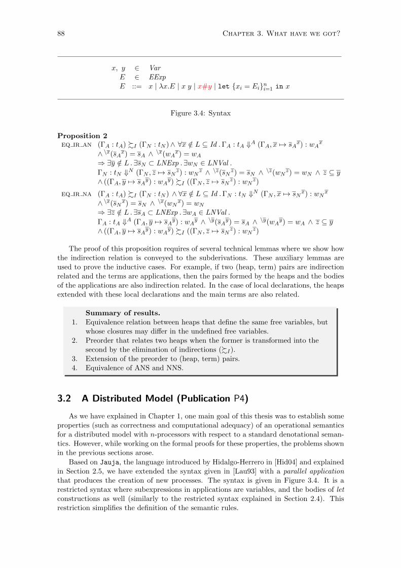
88 Chapter 3. What have we got?
x, y ∈ VarE ∈ EExpE ::= x | λx.E | x y | x#y | let {xi = Ei}ni=1 in x
Figure 3.4: Syntax
Proposition 2eq ir an (ΓA : tA) %I (ΓN : tN )∧ ∀x /∈ L ⊆ Id .ΓA : tA ⇓A (ΓA, x 7→ sA
x) : wAx
∧ \x(sAx) = sA ∧ \x(wA
x) = wA⇒ ∃y /∈ L .∃sN ⊂ LNExp .∃wN ∈ LNVal .
ΓN : tN ⇓N (ΓN , z 7→ sNz) : wN
z ∧ \z(sNz) = sN ∧ \z(wNz) = wN ∧ z ⊆ y∧ ((ΓA, y 7→ sA
y) : wAy) %I ((ΓN , z 7→ sN
z) : wNz)
eq ir na (ΓA : tA) %I (ΓN : tN ) ∧ ∀x /∈ L ⊆ Id .ΓN : tN ⇓N (ΓN , x 7→ sNx) : wN
x
∧ \x(sNx) = sN ∧ \x(wN
x) = wN⇒ ∃z /∈ L .∃sA ⊂ LNExp . ∃wA ∈ LNVal .
ΓA : tA ⇓A (ΓA, y 7→ sAy) : wA
y ∧ \y(sAy) = sA ∧ \y(wAy) = wA ∧ z ⊆ y∧ ((ΓA, y 7→ sA
y) : wAy) %I ((ΓN , z 7→ sN
z) : wNz)
The proof of this proposition requires of several technical lemmas where we show howthe indirection relation is conveyed to the subderivations. These auxiliary lemmas areused to prove the inductive cases. For example, if two (heap, term) pairs are indirectionrelated and the terms are applications, then the pairs formed by the heaps and the bodiesof the applications are also indirection related. In the case of local declarations, the heapsextended with these local declarations and the main terms are also related.
Summary of results.
1. Equivalence relation between heaps that define the same free variables, butwhose closures may differ in the undefined free variables.
2. Preorder that relates two heaps when the former is transformed into thesecond by the elimination of indirections (%I).
3. Extension of the preorder to (heap, term) pairs.4. Equivalence of ANS and NNS.
3.2 A Distributed Model (Publication P4)
As we have explained in Chapter 1, one main goal of this thesis was to establish someproperties (such as correctness and computational adequacy) of an operational semanticsfor a distributed model with n-processors with respect to a standard denotational seman-tics. However, while working on the formal proofs for these properties, the problems shownin the previous sections arose.
Based on Jauja, the language introduced by Hidalgo-Herrero in [Hid04] and explainedin Section 2.5, we have extended the syntax given in [Lau93] with a parallel applicationthat produces the creation of new processes. The syntax is given in Figure 3.4. It is arestricted syntax where subexpressions in applications are variables, and the bodies of letconstructions as well (similarly to the restricted syntax explained in Section 2.4). Thisrestriction simplifies the definition of the semantic rules.
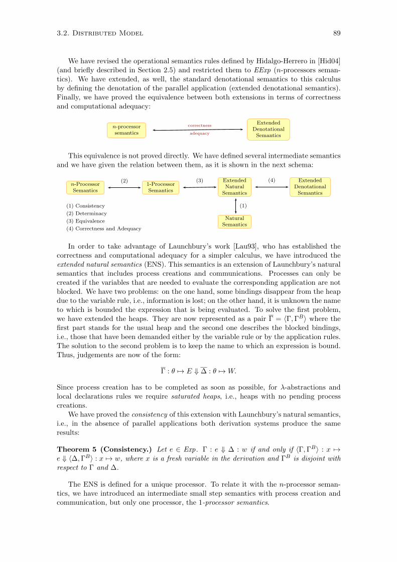
3.2. Distributed Model 89
We have revised the operational semantics rules defined by Hidalgo-Herrero in [Hid04](and briefly described in Section 2.5) and restricted them to EExp (n-processors seman-tics). We have extended, as well, the standard denotational semantics to this calculusby defining the denotation of the parallel application (extended denotational semantics).Finally, we have proved the equivalence between both extensions in terms of correctnessand computational adequacy:
n-processorsemantics
ExtendedDenotationalSemantics
correctness
adequacy
This equivalence is not proved directly. We have defined several intermediate semanticsand we have given the relation between them, as it is shown in the next schema:
n-ProcessorSemantics
1-ProcessorSemantics
ExtendedNatural
Semantics
NaturalSemantics
ExtendedDenotationalSemantics
(2) (3)
(1)
(4)
(1) Consistency
(2) Determinacy
(3) Equivalence
(4) Correctness and Adequacy
In order to take advantage of Launchbury’s work [Lau93], who has established thecorrectness and computational adequacy for a simpler calculus, we have introduced theextended natural semantics (ENS). This semantics is an extension of Launchbury’s naturalsemantics that includes process creations and communications. Processes can only becreated if the variables that are needed to evaluate the corresponding application are notblocked. We have two problems: on the one hand, some bindings disappear from the heapdue to the variable rule, i.e., information is lost; on the other hand, it is unknown the nameto which is bounded the expression that is being evaluated. To solve the first problem,we have extended the heaps. They are now represented as a pair Γ = 〈Γ,ΓB〉 where thefirst part stands for the usual heap and the second one describes the blocked bindings,i.e., those that have been demanded either by the variable rule or by the application rules.The solution to the second problem is to keep the name to which an expression is bound.Thus, judgements are now of the form:
Γ : θ 7→ E ⇓ ∆ : θ 7→W.
Since process creation has to be completed as soon as possible, for λ-abstractions andlocal declarations rules we require saturated heaps, i.e., heaps with no pending processcreations.
We have proved the consistency of this extension with Launchbury’s natural semantics,i.e., in the absence of parallel applications both derivation systems produce the sameresults:
Theorem 5 (Consistency.) Let e ∈ Exp. Γ : e ⇓ ∆ : w if and only if 〈Γ,ΓB〉 : x 7→e ⇓ 〈∆,ΓB〉 : x 7→ w, where x is a fresh variable in the derivation and ΓB is disjoint withrespect to Γ and ∆.
The ENS is defined for a unique processor. To relate it with the n-processor seman-tics, we have introduced an intermediate small step semantics with process creation andcommunication, but only one processor, the 1-processor semantics.

90 Chapter 3. What have we got?
S
H1 Hn
.
.
.. . .
.
.
.
HS
H1 ∪ . . . ∪ Hn
Figure 3.5: Coversion of a distributed system into a heap
SH
H1 Hn
x11 7→ E11
.
.
.x1m1
7→ E1m1
. . .
xn1 7→ En1
.
.
.xnmn
7→ Enmn
H
x11p17→ E11
.
.
.
x1m1
p17→ E1m1
. . .
xn1pn7→ En1
.
.
.
xnmn
pn7→ Enmn
Figure 3.6: Coversion of a non-distributed model into a distributed one
The n-processor semantics represents a distributive model with several processes thatevolve, at least, until the value for the main variable is obtained. Recall that there aretwo types of rules: the local rules that indicate the evolution inside each process; and theglobal rules to regulate process creations and communications. Each process is representedby a labelled heap. Since in the 1-processor semantics only one binding can be active atany time, we do not need to deal with the two levels. We just have local rules that forcean eager process creation and impose an order of evaluation that is compatible with theminimum semantics described in Section 2.5.1.
To prove that the n-processors semantics and the 1-processor semantics produce thesame value for the main variable, we need to construct a non-distributed model froma distributed one. For this purpose we build a unique heap that stores all the bindingsfrom the different processes. The potential active bindings become inactive except for one.This unique active binding is given by the function EB(H) that calculates the evolutionarybindings of a heap. This function depends on the semantics that is being used, in thiscase, the minimum semantics. Therefore, only one binding, that is directly demanded bythe main variable, can be active. Figure 3.5 shows the conversion of a distributed systeminto one heap.
To build a distributed system from a heap of bindings is more difficult. We need toknow to which process belongs each binding. This information is added to the bindings inthe form of an annotation. These annotations do not interfere with the semantic rules. Theschema shown in Figure 3.6 illustrates the conversion of a labelled heap into its associatedsystem.
The determinacy theorem establishes the equivalence between these two semanticswhen the minimum semantics is considered for the distributed model. Notice that systemsare represented as S = 〈pi, Hi〉ni=0, where a pair of the form 〈pi, Hi〉 represents a process(pi is the name of the process and Hi its heap).

3.2. Distributed Model 91
Γ = 〈Γ,ΓB〉
H = IB(H) ∪BB(H) ∪AB(H)
Figure 3.7: Conversion of heaps
Theorem 6 (Determinacy.) Let E ∈ EExp.
1. If 〈p0, {mainA7→ E}〉 =⇒∗ S =⇒∗ S′, then there exists a computation {main
A7→E} =⇒∗1 HS =⇒∗1 HS′, where HS (respectively HS′) is the heap constructed from S(respectively S′).
2. If {mainA7→ E} =⇒∗1 H =⇒∗1 H ′, then there exists a computation 〈p0, {main
A7→E}〉 =⇒∗ SH =⇒∗ SH′, where SH (respectively SH′) is the process system recoveredfrom heap H (respectively H ′).
Now, to prove the equivalence between the 1-processor semantics (small step semantics)and the extended natural semantics (big step semantics), we study the relation betweenthe labelled heaps produced by the 1-processor semantics and those of ENS. The inactivebindings of the heaps obtained by the small step semantics correspond to the first part ofthe extended heaps, while the blocked bindings correspond to the second part. Moreover,the unique active binding is the expression being evaluated. Conversely, we can constructa labelled heap for the 1-processor semantics from an extended heap. Figure 3.7 showshow to perform this conversion.
Now we are able to establish the equivalence theorem between these two semantics:
Theorem 7 (Equivalence ENS and 1-processor semantics.) Let E ∈ EExp.
1. If H + {θ A7→ E} ⇒∗1 H ′ + {θA7→ W}, then Γ : θ 7→ E ⇓ ∆ : θ 7→ W where Γ and ∆
are the extended heaps associated to H and H ′ respectively.
2. If Γ : θ 7→ E ⇓ ∆ : θ 7→ W , then H + {θ A7→ E} ⇒∗1 H ′ + {θA7→ W} where H and H ′
are the labelled heaps associated to Γ and ∆ respectively.
After dealing with the equivalence between the different operational semantics, we pro-ceed to prove the correctness and computational adequacy between the extended versionsof the natural semantics and the denotational semantics.
First, we briefly describe how we have extended Abramsky’s denotational semanticsto denotate channels and parallel applications. The new semantic function is:
[[−−]]ρ : EExp ∪ Chan → Env → Value
where ρ ∈ Env = Var ∪ Chan 7→ Value is an environment from identifiers to values. Thedenotation of a parallel application coincides with the denotation of an application, thatis, [[x#y]]ρ = [[x y]]ρ.
The correctness theorem establishes that the meaning of an expression does not changeduring its evaluation. Moreover, the size of heaps can only increase (new bindings may
92 Chapter 3. What have we got?
be added). A heap can be also modified by refining its bindings, that is, by updatingthe closures with the calculated values. We consider Heap as the domain of unlabelledheaps, i.e. sets of unlabelled bindings, and ρ ≤ ρ′ represents the order on environmentsdefined by Launchbury and explained in Section 2.4. We also consider the function {{. . .}} :Heap → Env → Env to extend an environment with the bindings of a heap (explained inSection 2.4).
Theorem 8 (Correctness of the extended natural semantics.)Let E ∈ EExp ∪ Chan, Γ = 〈Γ,ΓB〉, ∆ = 〈∆,∆B〉 ∈ EHeap, y θ /∈ dom(Γ).If Γ : θ 7→ E ⇓ ∆ : θ 7→ W , then for each environment ρ, [[E]]{{Γ}}ρ = [[W ]]{{∆}}ρ and{{Γ}}ρ ≤ {{∆}}ρ.
The computational adequacy determines that an expression reduces to a value if andonly if its denotation is not undefined.
Theorem 9 (Adequacy of the extended natural semantics.) Let E ∈ EExp∪Chan,Γ = 〈Γ,ΓB〉 ∈ EHeap, y θ /∈ dom(Γ). Γ : θ 7→ E ⇓ ∆ : θ 7→W , if and only if [[E]]{{Γ}}ρ 6=⊥.
The proofs of these last two theorems are done by following the steps given in [Lau93].The construction of these proofs have given rise to the study of the results presented inSection 3.1.
Summary of results.
1. Definition of a distributed operational semantics for n processors.2. Definition of a distributed operational semantics for a unique processor.3. Extension of the natural semantics with parallel applications.4. Consistency between the natural semantics and its extension.5. Equivalence between the 1-processor semantics and the parallel extension.6. Correctness of the extended natural semantics with respect to an extended
denotational semantics.
3.3 Related work
We have already said in Chapter 1 that several works have based on Launchbury’sresults [Lau93]. Breitner has also noticed, and he has developed in [Bre13, Bre14] aresearch to prove the correctness and computational adequacy of Launchbury’s naturalsemantics.
Breitner proposes two methods to prove the correctness of the natural semanticsin [Bre14]. The first one introduces an equivalent semantic to Launchbury’s one where the
judgments are of the form Γ : Γ′ W ∆ : ∆′, where Γ′ and ∆′ are ordered sets of bindings.These sets reflect how the evaluation of expressions is being demanded. Therefore, thesejudgments have more information than those of Launchbury. For instance, when evaluat-ing a variable, the corresponding binding will not disappear from the heap, it will be in Γ′.The idea is similar to the one explained in Section 3.2, where heaps are extended to keepthe information of the blocked bindings. As Breitner explains, in the case of Launchbury’ssemantics, only the topmost binding of the stack can change in each derivation rule. Heconsiders more natural this representation. He also thinks that it can be useful in othercases requiring the modification of the stack, for instance, by an extension with garbage
3.3. Related work 93
collection. In the second method, Breitner modifies the denotational semantics and rede-fines the function that relates the heaps with the environments (explained in Section 2.4),thus the operator for the least upper bound is replaced for a suitable update.
Some of our work related to publication P1 and explained in Section 3.1.1 has beenformalized in the proof assistant Isabelle by Breitner [Bre13]. He also proves the computa-tional adequacy of Launchbury’s natural semantics without using the alternative version.Recall that Launchbury introduced this version because the heaps of the operational se-mantics correspond to the environments of the denotational semantics. Breitner solvesthese problems in the denotational side, and do not need to prove the equivalence betweenthe original Launchbury’s natural semantics and the alternative natural semantics.
There is a correspondence between the locally nameless representation and the nominaltechniques as Breitner explains in [Bre14], since in both cases the names used in heaps areavoided.
Different methods and relations have been studied over the years to establish theequivalence between semantics. The work of Haeri [Hae09, Hae13] is related to ours insome aspects. He extends Launchbury’s language with a seq operator and defines a bigstep semantics for this construction. Based on this semantics, Haeri introduces threenotions of equivalence for expressions:
Value equivalence: Two expressions are value equivalent if they produce the samevalue when evaluated in the same initial context;
Heap equivalence: Two expressions are heap equivalent if they produce the samefinal heap when evaluated in the same initial context; and
Strict equivalence: Two expressions are strictly equivalent if they produce the samevalue and final heap when evaluated in the same initial context.
Although a number of interesting properties concerning the semantics are proved using thisequivalences, we have not used them because Haeri’s semantics differs from Launchbury’snatural semantics not only in the extension for seq, but also in the rule for local decla-rations. Following Launchbury, Haeri’s rule extends the heap with the local variables inorder to evaluate the body of the let-expression. But once the value is obtained, the localnames are removed from the heap. Therefore, the domains of the initial and final heapsare equal, and their differences come from the updating of closures. We are interested inrelating the semantics that Launchbury originally defined (without modifications); we haveonly changed its representation. Moreover, Haeri’s equivalences relate expressions usingthe same evaluation rules, while we relate expressions (and heaps) evaluated in differentreduction systems.
This idea of removing the local names once the body of a let-expression is evaluated,is also used by Haeri in [Hae13] for a distributed model that includes the operator #, thatrepresents strict application. Under this operator, the body of the application and its ar-gument are evaluated simultaneously with the same initial context, before the applicationis performed. A crucial difference with our distributed model, is that Haeri has a verylimited form of parallelism, and there is neither notion of process nor of communication.
To deal with the problems derived from α-conversion there exist other alternativesdifferent from the de Bruijn notation an the locally nameless representation explained inSection 2.6. Nowadays the nominal logic [Pit03, GP02] is one of the more popular ones.This logic is based on the fact that the syntactic properties are equivariant, i.e., theirvalidity is invariant under the (swapping) of names [Pit03].
94 Chapter 3. What have we got?
This logic does not only present advantages related with α-conversion problems, but itis also implemented in Isabelle, a very well known proof assistant. The nominal packageis being used in several studies although it is still a project under development [isa15].We chose the locally nameless representation because some years ago mutually recur-sive local declarations could present some problems in nominal Isabelle, and also becauseChargueraud’s work [Cha11] was very close to our purpose.
The study of Cimini et al. [CMRG12] on structural operational semantics uses sometechniques of the nominal logic and works with the notion of bisimilarity. Based on thenominal techniques introduced by Pitts, Gabbay and Urban [GP99, UPG04], the authorsdevelop the Nominal SOS (Nominal Structural Operational Semantics), and apply it tothe notion of nominal bisimilarity. Later on, they formulate the lazy λ-calculus using theNominal SOS and prove that it coincides with the original one. They also prove thatthe nominal bisimilarity coincides with Abramsky’s applicative bisimilarity explained inSection 2.3.3.
3.4 Conclusions
In this chapter we have shown the main results that we have obtained in the contextof this PhD thesis. We have started by relating two denotational semantics, a standardone and another with resources. This relation has been established by a similarity relationbetween the values of the domains of the respective semantics. These domains are D =[D → D]⊥ (as defined by Abramsky) for the standard denotational semantics, and E =[[C → E]→ [C → E]]⊥ for the semantics with resources, for which we have construct aninitial solution.
In order to prove the equivalence of Launchbury’s natural semantics with its alternativeversion we have introduce two intermediate semantics: one with indirections, and anotherwithout update. We have proved the equivalence between the alternative natural semanticsand the non-update version. To obtain this result we have defined a preorder, %I , betweenheaps. To establish this indirection relation we have previously defined some equivalencesbetween terms and heaps. Moreover, we have accomplished this work using a locallynameless representation.
Finally, we have considered a distributed model of the language with parallel applica-tions. To prove the correctness with respect to an extended denotational semantics (thatgives meaning to the new expressions), we have introduced two intermediate semantics:a 1-processor semantics and an extension of Launchbury’s natural semantics. We haveproved the consistency between the natural semantics and its extension, the equivalencebetween the 1-processor semantics and the extension of the natural semantics, and thecorrectness of the extended semantics with respect to an extension of the denotationalsemantics.
We itemize all the results that have been exposed in this chapter.
Construction of the initial solution of the domain equation E = [[C → E] → [C →E]]⊥, where C stands for the domain of resources.
Definition of the relation of similarity between the values of the domain E and thevalues of the standard function space D = [D → D]⊥.
Application of the previous result to prove the equivalence between the denotationalstandard semantics and the resourced denotational semantics for the lazy λ-calculus.

3.4. Conclusions 95
Locally nameless representation of the λ-calculus extended with recursive local dec-larations.
Locally nameless representation of Launchbury’s natural semantic rules and its al-ternative version.
Properties of the reduction systems (regularity, introduction and renaming).
Equivalence relation between heaps that define the same free variables, but whoseclosures may differ in the undefined free variables.
Preorder that relates two heaps when the former is transformed into the second bythe elimination of indirections (%I).
Extension of the preorder to (heap, term) pairs.
Equivalence of ANS and NNS.
Definition of a distributed operational semantics for n processors.
Definition of a distributed operational semantics for a unique processor.
Extension of the natural semantics with parallel applications.
Consistency between the natural semantics and its extension.
Equivalence between the 1-processor semantics and the parallel extension.
Correctness of the extended natural semantics with respect to an extended denota-tional semantics.

96 Chapter 3. What have we got?
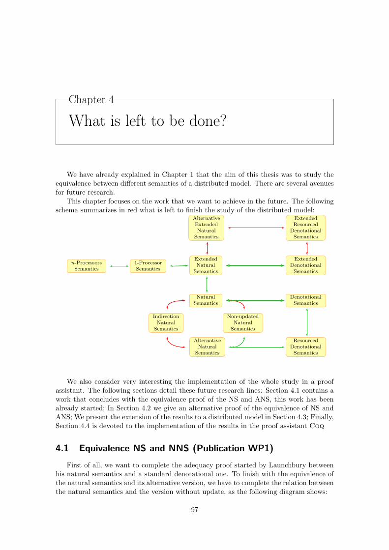
Chapter 4
What is left to be done?
We have already explained in Chapter 1 that the aim of this thesis was to study theequivalence between different semantics of a distributed model. There are several avenuesfor future research.
This chapter focuses on the work that we want to achieve in the future. The followingschema summarizes in red what is left to finish the study of the distributed model:
n-ProcessorsSemantics
1-ProcessorSemantics
ExtendedNatural
Semantics
NaturalSemantics
ExtendedDenotationalSemantics
IndirectionNatural
Semantics
Non-updatedNatural
Semantics
AlternativeNatural
Semantics
DenotationalSemantics
ResourcedDenotationalSemantics
ExtendedResourced
DenotationalSemantics
AlternativeExtendedNatural
Semantics
We also consider very interesting the implementation of the whole study in a proofassistant. The following sections detail these future research lines: Section 4.1 contains awork that concludes with the equivalence proof of the NS and ANS, this work has beenalready started; In Section 4.2 we give an alternative proof of the equivalence of NS andANS; We present the extension of the results to a distributed model in Section 4.3; Finally,Section 4.4 is devoted to the implementation of the results in the proof assistant Coq
4.1 Equivalence NS and NNS (Publication WP1)
First of all, we want to complete the adequacy proof started by Launchbury betweenhis natural semantics and a standard denotational one. To finish with the equivalence ofthe natural semantics and its alternative version, we have to complete the relation betweenthe natural semantics and the version without update, as the following diagram shows:
97

98 Chapter 4. What is left to be done?
NATURAL SEMANTICS(NS)
Indirections: NoUpdate: Yes
INDIRECTION NAT. SEM.(INS)
Indirections: YesUpdate: Yes
NON-UPDATE NAT. SEM. NAT.(NNS)
Indirections: NoUpdate: No
ALTERNATIVE NAT. SEM.(ANS)
Indirections: YesUpdate: No
We have already started with this study but we do not include it in this PhD becauseis not finished yet. The work in progress WP1 in Appendix B details what we have alreadyachieved. In this section we just describe the main ideas.
We start with an example to show the differences between the final heaps produced byevaluating an expression with NS and with NNS.
Example 9 Consider the following term:
t ≡ let abs (bvar 0 0), s, app (bvar 0 0) (bvar 0 1)in app (app (app (bvar 0 1) (bvar 0 0)) (bvar 0 0)) (bvar 0 2)
where
s ≡ let abs (bvar 0 0), abs (bvar 0 0), app (bvar 0 0) (bvar 0 1)in app (bvar 0 0) (bvar 0 1)
We evaluate the expression with NS (⇓) and NNS (⇓N ) in the context of an emptyheap. We obtain the following results:
{ } : t
⇓
x0 7→ abs (bvar 0 0),x1 7→ abs (bvar 0 0),x2 7→ abs (bvar 0 0),y0 7→ abs (bvar 0 0),y1 7→ abs (bvar 0 0),y2 7→ app (fvar y0) (fvar y1)
{ } : t
⇓N
x0 7→ abs (bvar 0 0),x1 7→ s,
x2 7→ app (fvar x0) (fvar x1),y0 7→ abs (bvar 0 0),y1 7→ abs (bvar 0 0),y2 7→ app (fvar y0) (fvar y1),z0 7→ abs (bvar 0 0),z1 7→ abs (bvar 0 0),z2 7→ app (fvar z0) (fvar z1)
w ≡ abs (bvar 0 0)
ut
Due to the absence of update in NNS, some parts of the computation are repeated. Thishappens when a variable is demanded more than once during the derivation. Therefore,some bindings are duplicated in the final heap but with different names. There are moredifferences between the final heaps. For instance, we also observe that some variables are
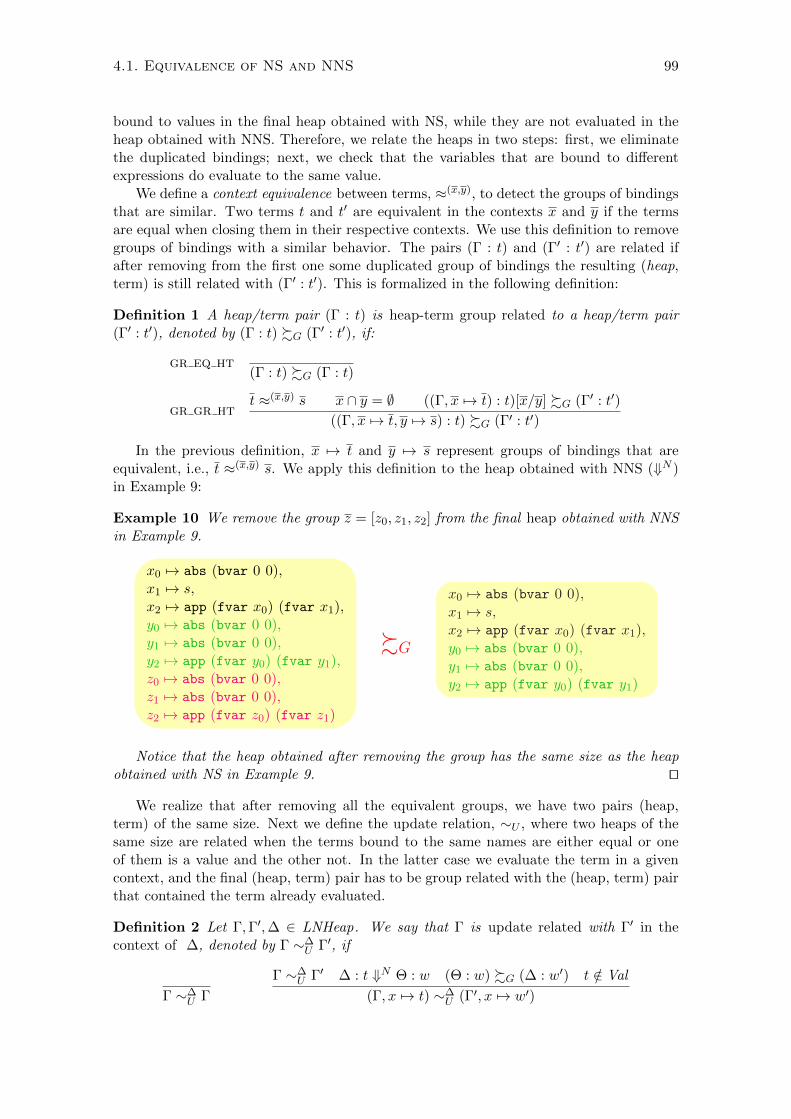
4.1. Equivalence of NS and NNS 99
bound to values in the final heap obtained with NS, while they are not evaluated in theheap obtained with NNS. Therefore, we relate the heaps in two steps: first, we eliminatethe duplicated bindings; next, we check that the variables that are bound to differentexpressions do evaluate to the same value.
We define a context equivalence between terms, ≈(x,y), to detect the groups of bindingsthat are similar. Two terms t and t′ are equivalent in the contexts x and y if the termsare equal when closing them in their respective contexts. We use this definition to removegroups of bindings with a similar behavior. The pairs (Γ : t) and (Γ′ : t′) are related ifafter removing from the first one some duplicated group of bindings the resulting (heap,term) is still related with (Γ′ : t′). This is formalized in the following definition:
Definition 1 A heap/term pair (Γ : t) is heap-term group related to a heap/term pair(Γ′ : t′), denoted by (Γ : t) %G (Γ′ : t′), if:
gr eq ht(Γ : t) %G (Γ : t)
gr gr htt ≈(x,y) s x ∩ y = ∅ ((Γ, x 7→ t) : t)[x/y] %G (Γ′ : t′)
((Γ, x 7→ t, y 7→ s) : t) %G (Γ′ : t′)
In the previous definition, x 7→ t and y 7→ s represent groups of bindings that areequivalent, i.e., t ≈(x,y) s. We apply this definition to the heap obtained with NNS (⇓N )in Example 9:
Example 10 We remove the group z = [z0, z1, z2] from the final heap obtained with NNSin Example 9.
x0 7→ abs (bvar 0 0),x1 7→ s,
x2 7→ app (fvar x0) (fvar x1),y0 7→ abs (bvar 0 0),y1 7→ abs (bvar 0 0),y2 7→ app (fvar y0) (fvar y1),z0 7→ abs (bvar 0 0),z1 7→ abs (bvar 0 0),z2 7→ app (fvar z0) (fvar z1)
%G
x0 7→ abs (bvar 0 0),x1 7→ s,
x2 7→ app (fvar x0) (fvar x1),y0 7→ abs (bvar 0 0),y1 7→ abs (bvar 0 0),y2 7→ app (fvar y0) (fvar y1)
Notice that the heap obtained after removing the group has the same size as the heapobtained with NS in Example 9. ut
We realize that after removing all the equivalent groups, we have two pairs (heap,term) of the same size. Next we define the update relation, ∼U , where two heaps of thesame size are related when the terms bound to the same names are either equal or oneof them is a value and the other not. In the latter case we evaluate the term in a givencontext, and the final (heap, term) pair has to be group related with the (heap, term) pairthat contained the term already evaluated.
Definition 2 Let Γ,Γ′,∆ ∈ LNHeap. We say that Γ is update related with Γ′ in thecontext of ∆, denoted by Γ ∼∆
U Γ′, if
Γ ∼∆U Γ
Γ ∼∆U Γ′ ∆ : t ⇓N Θ : w (Θ : w) %G (∆ : w′) t /∈ Val
(Γ, x 7→ t) ∼∆U (Γ′, x 7→ w′)
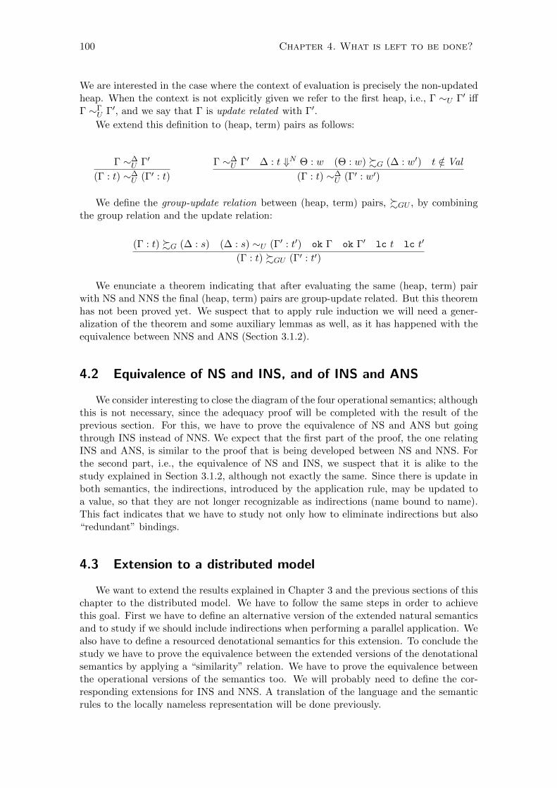
100 Chapter 4. What is left to be done?
We are interested in the case where the context of evaluation is precisely the non-updatedheap. When the context is not explicitly given we refer to the first heap, i.e., Γ ∼U Γ′ iffΓ ∼Γ
U Γ′, and we say that Γ is update related with Γ′.
We extend this definition to (heap, term) pairs as follows:
Γ ∼∆U Γ′
(Γ : t) ∼∆U (Γ′ : t)
Γ ∼∆U Γ′ ∆ : t ⇓N Θ : w (Θ : w) %G (∆ : w′) t /∈ Val
(Γ : t) ∼∆U (Γ′ : w′)
We define the group-update relation between (heap, term) pairs, %GU , by combiningthe group relation and the update relation:
(Γ : t) %G (∆ : s) (∆ : s) ∼U (Γ′ : t′) ok Γ ok Γ′ lc t lc t′
(Γ : t) %GU (Γ′ : t′)
We enunciate a theorem indicating that after evaluating the same (heap, term) pairwith NS and NNS the final (heap, term) pairs are group-update related. But this theoremhas not been proved yet. We suspect that to apply rule induction we will need a gener-alization of the theorem and some auxiliary lemmas as well, as it has happened with theequivalence between NNS and ANS (Section 3.1.2).
4.2 Equivalence of NS and INS, and of INS and ANS
We consider interesting to close the diagram of the four operational semantics; althoughthis is not necessary, since the adequacy proof will be completed with the result of theprevious section. For this, we have to prove the equivalence of NS and ANS but goingthrough INS instead of NNS. We expect that the first part of the proof, the one relatingINS and ANS, is similar to the proof that is being developed between NS and NNS. Forthe second part, i.e., the equivalence of NS and INS, we suspect that it is alike to thestudy explained in Section 3.1.2, although not exactly the same. Since there is update inboth semantics, the indirections, introduced by the application rule, may be updated toa value, so that they are not longer recognizable as indirections (name bound to name).This fact indicates that we have to study not only how to eliminate indirections but also“redundant” bindings.
4.3 Extension to a distributed model
We want to extend the results explained in Chapter 3 and the previous sections of thischapter to the distributed model. We have to follow the same steps in order to achievethis goal. First we have to define an alternative version of the extended natural semanticsand to study if we should include indirections when performing a parallel application. Wealso have to define a resourced denotational semantics for this extension. To conclude thestudy we have to prove the equivalence between the extended versions of the denotationalsemantics by applying a “similarity” relation. We have to prove the equivalence betweenthe operational versions of the semantics too. We will probably need to define the cor-responding extensions for INS and NNS. A translation of the language and the semanticrules to the locally nameless representation will be done previously.

4.4. Implementation in Coq 101
4.4 Implementation in Coq (Publication WP2)
Automated theorem provers and proof assistants, that have been introduced in Sec-tion 2.7, are well known for their reliability in formal proofs. We find of great importanceto use one of them to implement the work done in this thesis.
When we started working with Isabelle, the Nominal package was in its origins andthe use of mutually recursive local declarations was problematic. Without this nominalpackage we had to work with the de Bruijn notation. We explained in Section 2.6.1 thedisadvantages of this notation.
By contrast, Coq deals well with inductive definitions and allowed to work with re-cursive local declarations. Moreover, there existed some works using the locally namelessrepresentation [Cha11] with Coq. This was the main reason to choose this proof assistant.
Although the language that we use has applications restricted to variables (Figure 3.2),we decided to work with applications from terms to terms in Coq. To extend the workof Chargueraud [Cha11], we have extended the definition of the language with recursivelocal declarations represented by a list of terms:
Inductive trm : Type :=| t bvar : nat− > nat− > trm
| t fvar : var− > trm
| t abs : trm− > trm
| t app : trm− > trm− > trm
| t let : L trm− > trm− > trm
with L trm :=| nil Lt : L trm
| cons Lt : trm− > L trm− > L trm.
But the induction principle that Coq defines is not transmitted to the list of terms,as it only verifies the property for the main term of the local declarations. This can beseen when checking for the induction principle in Coq:
trm ind : forall P : trm − > Prop,(forall n n0 : nat, P (trm bvar n n0)) − >(forall v : var, P (trm fvar v)) − >(forall t : trm, P t − > P (trm abs t)) − >(forall t : trm, P t − > forall t0 : trm, P t0 − > P (trm app t t0)) − >(forall (l : L trm) (t : trm), P t − > P (trm let l t)) − >forall t : trm, P t
Therefore, we have redefined this principle. There are two mutually recursive proper-ties: P for the terms and P0 for the lists.
trm ind2 forall (P : trm − > Prop) (P0 : L trm − > Prop),(forall n n0 : nat, P (trm bvar n n0)) − >(forall v : var, P (trm fvar v)) − >(forall t : trm, P t − > P (trm abst)) − >(forall t : trm, P t − > forall t0 : trm, P t0 − > P (trm app t t0)) − >(forall l : L trm, P0 l − > forall t : trm, P t − > P (trm let l t)) − >P0 nil Ltrm − >(forall t : trm, P t − > forall l : L trm, P0 l − > P0 (cons Ltrm t l)) − >forall t : trm, P t
Once we fixed the problems with the induction principle, we have extended somedefinitions such as variable opening, variable closing, substitution and free variables of a
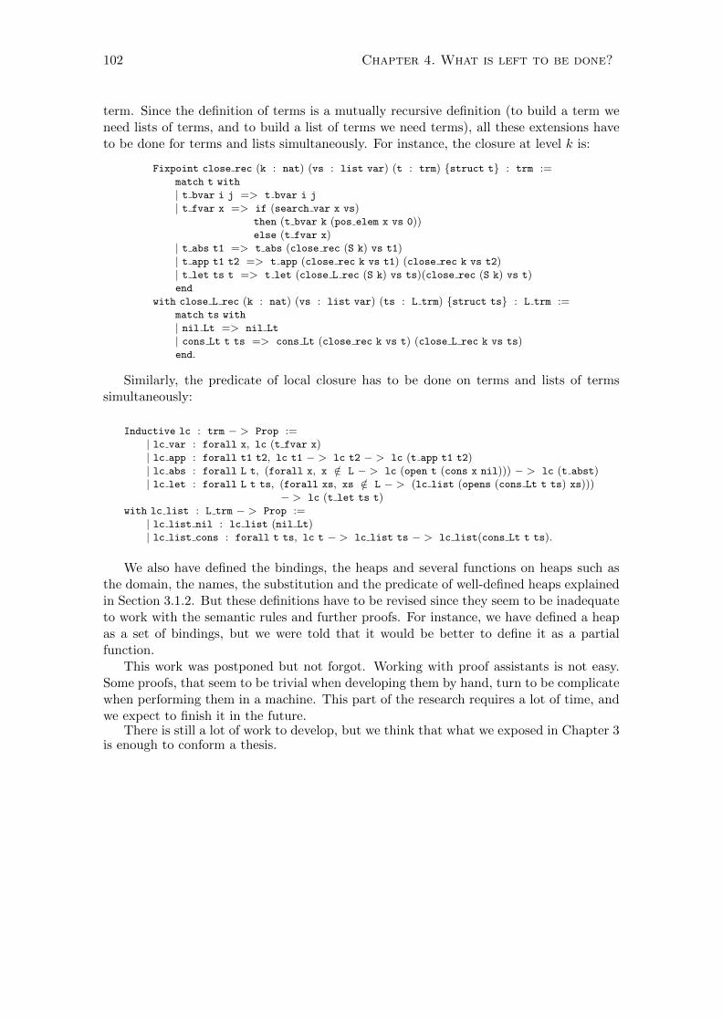
102 Chapter 4. What is left to be done?
term. Since the definition of terms is a mutually recursive definition (to build a term weneed lists of terms, and to build a list of terms we need terms), all these extensions haveto be done for terms and lists simultaneously. For instance, the closure at level k is:
Fixpoint close rec (k : nat) (vs : list var) (t : trm) {struct t} : trm :=match t with
| t bvar i j => t bvar i j
| t fvar x => if (search var x vs)then (t bvar k (pos elem x vs 0))else (t fvar x)
| t abs t1 => t abs (close rec (S k) vs t1)| t app t1 t2 => t app (close rec k vs t1) (close rec k vs t2)| t let ts t => t let (close L rec (S k) vs ts)(close rec (S k) vs t)end
with close L rec (k : nat) (vs : list var) (ts : L trm) {struct ts} : L trm :=match ts with
| nil Lt => nil Lt
| cons Lt t ts => cons Lt (close rec k vs t) (close L rec k vs ts)end.
Similarly, the predicate of local closure has to be done on terms and lists of termssimultaneously:
Inductive lc : trm − > Prop :=| lc var : forall x, lc (t fvar x)| lc app : forall t1 t2, lc t1 − > lc t2 − > lc (t app t1 t2)| lc abs : forall L t, (forall x, x /∈ L − > lc (open t (cons x nil))) − > lc (t abst)| lc let : forall L t ts, (forall xs, xs /∈ L − > (lc list (opens (cons Lt t ts) xs)))
− > lc (t let ts t)with lc list : L trm − > Prop :=
| lc list nil : lc list (nil Lt)| lc list cons : forall t ts, lc t − > lc list ts − > lc list(cons Lt t ts).
We also have defined the bindings, the heaps and several functions on heaps such asthe domain, the names, the substitution and the predicate of well-defined heaps explainedin Section 3.1.2. But these definitions have to be revised since they seem to be inadequateto work with the semantic rules and further proofs. For instance, we have defined a heapas a set of bindings, but we were told that it would be better to define it as a partialfunction.
This work was postponed but not forgot. Working with proof assistants is not easy.Some proofs, that seem to be trivial when developing them by hand, turn to be complicatewhen performing them in a machine. This part of the research requires a lot of time, andwe expect to finish it in the future.
There is still a lot of work to develop, but we think that what we exposed in Chapter 3is enough to conform a thesis.
Bibliografıa
[Abr90] S. Abramsky. Research Topics in Functional Programming, chapter 4: The lazylambda calculus, pages 65–117. Ed. D. A. Turner. Addison Wesley, 1990.
[Abr91] S. Abramsky. Domain theory in logical form*. Annals of Pure and Applied Logic,51(1-2):1 – 77, 1991.
[ACP+08] B. E. Aydemir, A. Chargueraud, B. C. Pierce, R. Pollack, and S. Weirich. En-gineering formal metatheory. In ACM Symposium on Principles of ProgrammingLanguages, POPL’08, pages 3–15. ACM Press, 2008.
[agd14] Agda. http://wiki.portal.chalmers.se/agda/pmwiki.php, 2014. Accedido30-10-2014.
[AJ94] S. Abramsky and A. Jung. Domain theory. In Handbook of Logic in ComputerScience (Vol. 3), pages 1–168. Oxford University Press, 1994.
[AO93] S. Abramsky and L. Ong. Full abstraction in the lazy lambda calculus. Informationand Computation, 105(2):159–267, 1993.
[Bar84] H. P. Barendregt. The Lambda Calculus: Its Syntax and Semantics, volume 103of Studies in Logic and the Foundations of Mathematics. North-Holland, 1984.
[BB00] H. Barendregt and E. Barendsen. Introduction to lambda calculus, 2000.
[BKT00] C. Baker-Finch, D. King, and P. W. Trinder. An operational semantics for para-llel lazy evaluation. In ACM-SIGPLAN International Conference on FunctionalProgramming ICFP’00, pages 162–173. ACM Press, 2000.
[BLOP96] S. Breitinger, R. Loogen, Y. Ortega-Mallen, and R. Pena. Eden: Lan-guage definition and operational semantics. Technical Report 96/10, ReiheInformatik, FB Mathematik, Philipps-Universitat Marburg, Germany, URLhttp://www.mathematik.uni-marburg.de/∼eden/, 1996.
[Bre13] J. Breitner. The correctness of Launchbury’s natural semantics for lazy evalua-tion. Archive of Formal Proofs, January 2013. http://afp.sf.net/entries/
Launchbury.shtml, Formal proof development.
[Bre14] J. Breitner. The correctness of Launchbury’s natural semantics for lazy evaluation.arXiv:1405.3099v1, 2014.
[Cha11] A. Chargueraud. The locally nameless representation. Journal of AutomatedReasoning, pages 1–46, 2011.
[CMRG12] M. Cimini, M. R. Mousavi, M. A. Reniers, and M. J. Gabbay. Nominal SOS.Electronic Notes in Theoretical Computer Science, 286:103–116, 2012.
[Col89] M. Cole. Algorithmic Skeletons: Structured Management of Parallel Computation.Research Monographs in Parallel and Distributed Computing. Pitman, 1989.
[coq14] The Coq proof assistant. http://coq.inria.fr/, 2014. Accedido 30-10-2014.
103
104 BIBLIOGRAFIA
[dB72] N. G. de Bruijn. Lambda calculus notation with nameless dummies, a tool forautomatic formula manipulation, with application to the Church-Rosser theorem.Indagationes Mathematicae, 75(5):381–392, 1972.
[ede14] Eden. http://www.mathematik.uni-marburg.de/~eden/, 2014. Accedido 15-12-2014.
[erl14a] Erlang solutions. https://www.erlang-solutions.com/industries, 2014. Ac-cedido 30-10-2014.
[erl14b] What is Erlang. https://www.erlang.org/faq/introduction.html, 2014. Ac-cedido 30-10-2014.
[Esp14] Real Academia Espanola. Diccionario de la lengua espanola (22.a edicion). http://www.rae.es/recursos/diccionarios/drae, 2014. Accedido 30-10-2014.
[Geu09] H. Geuvers. Proof assistants: History, ideas and future. Sadhana, 34(1):3–25,February 2009.
[Gor94] A. D. Gordon. A mechanisation of name-carrying syntax up to alpha-conversion.In International Workshop on Higher Order Logic Theorem Proving and its Ap-plications, HUG ’93, pages 413–425. LNCS 780, Springer-Verlag, 1994.
[GP99] M. J. Gabbay and A. M. Pitts. A new approach to abstract syntax involvingbinders. In Annual Symposium on Logic in Computer Science, pages 214–224.IEEE Computer Society Press, 1999.
[GP02] M. J. Gabbay and A. M. Pitts. A new approach to abstract syntax with variablebinding. Formal Aspects of Computing, 13(3–5):341–363, 2002.
[Hae09] S. H. Haeri. Reasoning about selective strictness. Master’s thesis, School of Mat-hematical and Computer Sciences, Heriot-Watt University, 2009.
[Hae13] S. H. Haeri. A new operational semantics for distributed lazy evaluation. Te-chnical Report TR2013-1, Institute for Software Systems, Technische UniversitatHamburg, 2013.
[has14a] Haskell in industry. https://www.haskell.org/haskellwiki/Haskell_in_
industry, 2014. Accedido 30-10-2014.
[has14b] The haskell programming language. https://www.haskell.org/haskellwiki/
Haskell, 2014. Accedido 30-10-2014.
[has15] Lazy evaluation. https://wiki.haskell.org/Lazy_evaluation, 2015. Accedido14-05-2015.
[Hid04] M. Hidalgo-Herrero. Semanticas formales para un lenguaje funcional paralelo. PhDthesis, Dept. Sistemas Informaticos y Programacion, Universidad Complutense deMadrid, 2004.
[HO02] M. Hidalgo-Herrero and Y. Ortega-Mallen. An operational semantics for the pa-rallel language Eden. In International Workshop on Constructive Methods forParallel Programming, CMPP’02, pages 63–79. Technische Universitaet Berlin,Germany, 2002.
[isa14] Isabelle. http://isabelle.in.tum.de/, 2014. Accedido 30-10-2014.
[isa15] Nominal Isabelle. http://isabelle.in.tum.de/nominal/, 2015. Accedido 22-01-2015.
[Lau93] J. Launchbury. A natural semantics for lazy evaluation. In ACM Symposium onPrinciples of Programming Languages, (POPL’93), pages 144–154. ACM Press,1993.
[Ler07] X. Leroy. A locally nameless solution to the POPLmark challenge. Technicalreport, INRIA, January 2007.
BIBLIOGRAFIA 105
[Loo99] R. Loogen. Research Directions in Parallel Functional Programming, chapter 3:Programming Language Constructs, pages 63–92. Eds. K. Hammond and G. Mi-chaelson. Springer-Verlag, 1999.
[LOP05] R. Loogen, Y. Ortega-Mallen, and R. Pena. Parallel functional programming inEden. Journal of Functional Programming, 15(3):431–475, 2005.
[mir15] Miranda. http://http://miranda.org.uk/, 2015. Accedido 14-05-2015.
[MTH90] R. Milner, M. Tofte, and R. Harper. The definition of Standard ML. MIT Press,1990.
[NH09] K. Nakata and M. Hasegawa. Small-step and big-step semantics for call-by-need.CoRR, abs/0907.4640, 2009.
[OSV10] M. Odersky, L. Spoon, and B. Venners. Programming in Scala. Artima, 2010.
[Pey03] S. L. Peyton Jones. Haskell 98 language and libraries: the Revised Report. Cam-bridge University Press, 2003.
[Pit03] A. M. Pitts. Nominal logic, a first order theory of names and binding. Informationand Computation, 186(2):165–193, 2003.
[Pit13] A. M. Pitts. Nominal Sets: Names and Symmetry in Computer Science. Cam-bridge University Press, 2013.
[pvs14] PVS specification and verification system. http://pvs.csl.sri.com/, 2014. Ac-cedido 30-10-2014.
[Rea89] C. Reade. Elements of Functional Programming. Addison-Wesley, 1989.
[Sco73] D. Scott. Models for various type-free calculi. Logic, Methodology, and Philosophyof Science IV, pages 157–187, 1973.
[Ses97] P. Sestoft. Deriving a lazy abstract machine. Journal of Functional Programming,7(3):231–264, 1997.
[SGHHOM10] L. Sanchez-Gil, M. Hidalgo-Herrero, and Y. Ortega-Mallen. Trends in FunctionalProgramming, volume 10, chapter An Operational Semantics for Distributed LazyEvaluation, pages 65–80. Intellect, 2010.
[SGHHOM11] L. Sanchez-Gil, M. Hidalgo-Herrero, and Y. Ortega-Mallen. Relating functionspaces to resourced function spaces. In ACM Symposium on Applied Computing,SAC ’11, pages 1301–1308. ACM Press, 2011.
[SGHHOM12a] L. Sanchez-Gil, M. Hidalgo-Herrero, and Y. Ortega-Mallen. A formalization inCoq of Launchbury’s natural semantics for lazy evaluation. In Jornadas sobreProgramacion y Lenguajes, PROLE’12, pages 15–29, 2012.
[SGHHOM12b] L. Sanchez-Gil, M. Hidalgo-Herrero, and Y. Ortega-Mallen. A locally namelessrepresentation for a natural semantics for lazy evaluation. In International Collo-quium Theoretical Aspects of Computing, ICTAC’12, pages 105–119. LNCS 7521,Springer-Verlag, 2012.
[SGHHOM12c] L. Sanchez-Gil, M. Hidalgo-Herrero, and Y. Ortega-Mallen. A locally namelessrepresentation for a natural semantics for lazy evaluation. Technical Report 01/12,Dpt. Sistemas Informaticos y Computacion. Univ. Complutense de Madrid, 2012.http://federwin.sip.ucm.es/sic/investigacion/publicaciones/pdfs/SIC-1-12.pdf.
[SGHHOM13] L. Sanchez-Gil, M. Hidalgo-Herrero, and Y. Ortega-Mallen. The role of indi-rections in lazy natural semantics (extended version). Technical Report 13/13,Dpt. Sistemas Informaticos y Computacion. Univ. Complutense de Madrid, 2013.http://federwin.sip.ucm.es/sic/investigacion/publicaciones/pdfs/TR-13-13.pdf.
106 BIBLIOGRAFIA
[SGHHOM14a] L. Sanchez-Gil, M. Hidalgo-Herrero, and Y. Ortega-Mallen. Launchbury’s seman-tics revisited: On the equivalence of context-heap semantics. In Jornadas sobreProgramacion y Lenguajes, PROLE’14, pages 203–217, 2014.
[SGHHOM14b] L. Sanchez-Gil, M. Hidalgo-Herrero, and Y. Ortega-Mallen. The role of indirec-tions in lazy natural semantics. In PSI, 2014. Pendiente de publicacion en LNCS,Springer-Verlag.
[THLP98] P. W. Trinder, K. Hammond, H. W. Loidl, and S. L. Peyton Jones. Algorithm +Strategy = Parallelism. Journal of Funcional Programming, 8(1):23–60, 1998.
[TLP03] P. W. Trinder, H. W. Loidl, and R. F. Pointon. Parallel and Distributed Haskells.Journal of Functional Programming, 12(4+5):469–510, 2003.
[UBN07] C. Urban, S. Berghofer, and M. Norrish. Barendregt’s variable convention in ruleinductions. In International Conference on Automated Deduction, pages 35–50.LNCS 4603, Springer-Verlag, 2007.
[UPG04] C. Urban, A. M. Pitts, and M. Gabbay. Nominal unification. Theoretical ComputerScience, 323(1-3):473–497, 2004.
[vEdM07] M. van Eekelen and M. de Mol. Reflections on Type Theory, λ-calculus, and theMind. Essays dedicated to Henk Barendregt on the Occasion of his 60th Birthday,chapter Proving Lazy Folklore with Mixed Lazy/Strict Semantics, pages 87–101.Radboud University Nijmegen, 2007.
[wha14] Codigo abierto de whatsapp. https://www.whatsapp.com/opensource/, 2014.Accedido 30-10-2014.
[Wie06] F. Wiedijk, editor. The Seventeen Provers of the World, Foreword by Dana S.Scott. LNCS 3600, Springer-Verlag, 2006.
[Win93] G. Winskel. The Formal Semantics of Programming Languages: An Introduction.MIT Press, 1993.

Parte III
Publicaciones
107


Capıtulo 5
Publicaciones
Este capıtulo contiene las cuatro publicaciones principales que forman la tesis. Al igualque se hizo en el Capıtulo 3, las publicaciones aparecen de forma tematica en lugar decronologicamente.
En primer lugar presentamos el artıculo P1 [SGHHOM11] sobre la construccion dedominios, semanticas denotacionales y su relacion mediante bisimilitud. El trabajo fuepresentado en el 26th Symposium on Applied Computing (SAC) que tuvo lugar en Taichung(Taiwan) en septiembre de 2011, y fue publicado por ACM en las actas del simposium.
A continuacion hay un bloque de dos artıculos relacionados con la demostracion de laequivalencia entre las dos semanticas operacionales presentadas por Launchbury [Lau93].La primera publicacion de este bloque, P2 [SGHHOM12b], contiene la representacionlocalmente sin nombres de la semantica natural y la demostracion de diversas propiedadesrelacionadas con esta representacion. Esta representacion facilita las demostraciones de losresultados que se exponen en la segunda publicacion. El artıculo sobre la representacionlocalmente sin nombres se presento en el 9th International Colloquium on TheoreticalAspects of Computing (ICTAC) en Bangalore (India) en septiembre de 2012 y se publico enel volumen 7521 de la serie LNCS de Springer-Verlag. En cuanto al segundo artıculo deeste bloque, P3 [SGHHOM14b], se presento en la novena edicion de Perspectives of SystemInformatics (PSI) en San Petersburgo (Rusia) en junio de 2014 y se publico en el volumen8974 de la serie LNCS de Springer-Verlag. En este artıculo se hace un estudio sobre elpapel que juegan las indirecciones a lo largo de una evaluacion, y se establece una relacionentre los contextos y los valores obtenidos al evaluar un mismo termino con dos semanticasdistintas, una de las cuales introduce indirecciones.
Cierra el capıtulo la publicacion P4 [SGHHOM10] en la que se hace un estudio dedistintas semanticas sobre un modelo distribuido. Este trabajo fue presentado en junio de2009 en el 10th Trends in Functional Programming celebrado en Komarno (Eslovaquia), yposteriormente seleccionado para su publicacion en el volumen 10 de Trends in FunctionalProgramming, Intellect.
This chapter contains the main publications that form this thesis. As we have done inChapter 3, these publications are presented according to their thematic.
The first paper, P1 [SGHHOM11], is about domain construction, denotational seman-tics and their relation through bisimilarity. This was presented in the 26th Symposium onApplied Computing (SAC) in Taichung (Taiwan) in September 2011. This was publishedby ACM in the proceedings of the symposium.
Next, there are two papers devoted to the missing proof of Launchbury’s work. The
109
110 Capıtulo 5. Publicaciones
first one, P2 [SGHHOM12b], focuses on the locally nameless representation of the naturalsemantics for lazy evaluation. Some properties of this representation are proved as well.This work is useful for the development of the proofs of the second paper. This paperwas presented in the 9th International Colloquium on Theoretical Aspects of Computing(ICTAC) in Bangalore (India) in September 2012 and was published in the volume 7521of the LNCS by Springer-Verlag. The second work, P3 [SGHHOM14b], was presented inthe 9th Perspectives of System Informatics (PSI) in Saint Petersburg (Russia) in June2014 and was published in the volume 8974 of the LNCS by Springer-Verlag. In this workwe study the role of indirections during the evaluation. We define a relation between thecontext and value obtained when an expression is evaluated with two different semantics.
The last publication, P4 [SGHHOM10], is dedicated to a distributed model, where therelation between several semantics is shown. This paper was presented in the 10th Trendsin Functional Programming in Komarno (Slovakia), and it was published in volume 10 ofTrends in Functional Programming by Intellect.

Relating function spaces to resourced function spaces
Lidia Sánchez-GilUniversidad Complutense de
MercedesHidalgo-Herrero
Universidad Complutense deMadrid
Yolanda Ortega-MallénUniversidad Complutense de
ABSTRACTIn order to prove the computational adequacy of the (oper-ational) natural semantics for lazy evaluation with respectto a standard denotational semantics, Launchbury definesa resourced denotational semantics. This should be equiva-lent to the standard one when given infinite resources, butthis fact cannot be so directly established, because each se-mantics produces values in a different domain. The valuesobtained by the standard semantics belong to the usual liftedfunction space D = [D → D]⊥, while those produced by theresourced semantics belong to [C → E] where E satisfies theequation E = [[C → E] → [C → E]]⊥ and C (the domain ofresources) is a countable chain domain defined as the leastsolution of the domain equation C = C⊥.We propose a way to relate functional values in the stan-
dard lifted function space to functional values in the corre-sponding resourced function space. We first construct theinitial solution for the domain equation E = [[C → E] →[C → E]]⊥ following Abramsky’s construction of the initialsolution of D = [D → D]⊥. Then we define a “similarity”relation between values in the constructed domain and val-ues in the standard lifted function space. This relation isinspired by Abramsky’s applicative bisimulation.Finally we prove the desired equivalence between the stan-
dard denotational semantics and the resourced semantics forthe lazy λ-calculus.
Categories and Subject DescriptorsD.3.1 [Programming Languages]: Formal Definitions andTheory—semantics
KeywordsDomain theory, denotational semantics, λ-calculus.
1. MOTIVATIONThere is a mismatch between the pure λ-calculus in the
standard theory [4] and the practice of functional program-
Permission to make digital or hard copies of all or part of this work forpersonal or classroom use is granted without fee provided that copies arenot made or distributed for profit or commercial advantage and that copiesbear this notice and the full citation on the first page. To copy otherwise, torepublish, to post on servers or to redistribute to lists, requires prior specificpermission and/or a fee.SAC’11 March 21-25, 2011, TaiChung, Taiwan.Copyright 2011 ACM 978-1-4503-0113-8/11/03 ...$10.00.
ming, or more precisely, the lazy functional languages. Thissituation has been pointed out clearly by Abramsky in hisseminal paper [1], where he proposes a“lazy”theory based onthe notion of applicative transition systems and introduces asuitable domain equation, i.e., D = [D → D]⊥, which has anontrivial initial solution that constitutes a canonical modelfor the family of lazy languages. The construction of thisinitial solution is detailed in [2]. We adapt this constructionto the case where resources are added to the computationalmodel, so that we obtain the initial solution for the domainequation E = [[C → E] → [C → E]]⊥, where C is a count-able chain domain defined as the least solution of the domainequation C = C⊥.“Resourced” domains like E enable to define semantics
that restrict the number of available resources. For instance,let us consider that only 60 seconds of CPU time are avail-able and that each reduction needs one second; thus after 60reductions the system gets blocked and the semantic value is⊥. Another example: Boudol, Curien and Lavatelli presentin [5] a λ-calculus with resources to provide a control on thesubstitution process, so that a computation gets in deadlockwhen there are not enough resources to carry out all thesubstitutions. For this they use a different domain equa-tion, namely D = [M(D) → D]⊥, where M(D) stands formultisets of D.
The resourced domain E was used by Launchbury in [7]to define a (denotational) resourced semantics that was in-troduced to prove the computational adequacy of his (op-erational) natural semantics for lazy evaluation. In thatresourced semantics each syntactic level (in the term to beevaluated) requires the consumption of one resource. Thismimics the derivation process for the natural semantics,where one operational rule is applied to eliminate each syn-tactic level. Hence, denotations that consume a finite num-ber of resources correspond to finite derivations. Neverthe-less, the construction of the initial solution for the domainequation E = [[C → E] → [C → E]]⊥ is not detailed inLaunchbury’s work, and we have found it described nowhere.
Our motivation for constructing an initial solution forE = [[C → E] → [C → E]]⊥ (let us call it CValue) isto define a correspondence between its elements and thoseof the lifted function space D = [D → D]⊥ (let us callit Value). This correspondence is necessary to prove that,provided an unbounded number of resources, the resourcedsemantics equals the standard denotational semantics. In[7] Launchbury simply states that both semantics computethe same values, but this is not exact because the valuesproduced by the standard semantics belong to Value, while
1301
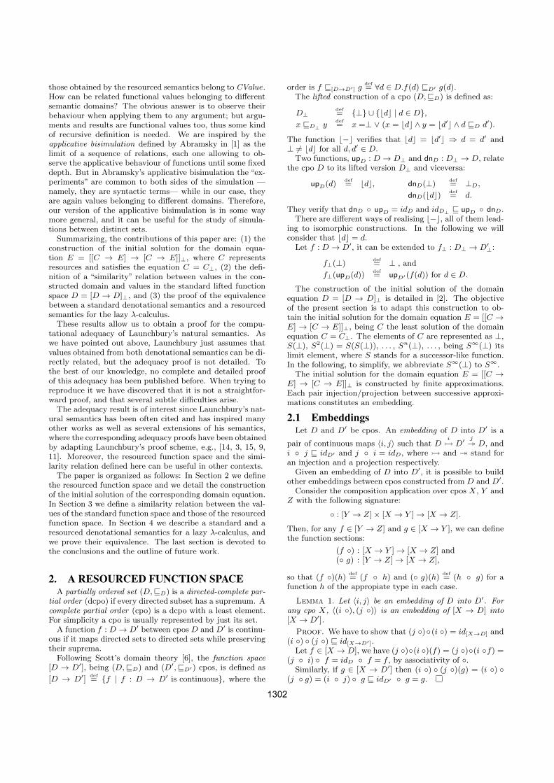
those obtained by the resourced semantics belong to CValue.How can be related functional values belonging to differentsemantic domains? The obvious answer is to observe theirbehaviour when applying them to any argument; but argu-ments and results are functional values too, thus some kindof recursive definition is needed. We are inspired by theapplicative bisimulation defined by Abramsky in [1] as thelimit of a sequence of relations, each one allowing to ob-serve the applicative behaviour of functions until some fixeddepth. But in Abramsky’s applicative bisimulation the “ex-periments” are common to both sides of the simulation —namely, they are syntactic terms— while in our case, theyare again values belonging to different domains. Therefore,our version of the applicative bisimulation is in some waymore general, and it can be useful for the study of simula-tions between distinct sets.Summarizing, the contributions of this paper are: (1) the
construction of the initial solution for the domain equa-tion E = [[C → E] → [C → E]]⊥, where C representsresources and satisfies the equation C = C⊥, (2) the defi-nition of a “similarity” relation between values in the con-structed domain and values in the standard lifted functionspace D = [D → D]⊥, and (3) the proof of the equivalencebetween a standard denotational semantics and a resourcedsemantics for the lazy λ-calculus.These results allow us to obtain a proof for the compu-
tational adequacy of Launchbury’s natural semantics. Aswe have pointed out above, Launchbury just assumes thatvalues obtained from both denotational semantics can be di-rectly related, but the adequacy proof is not detailed. Tothe best of our knowledge, no complete and detailed proofof this adequacy has been published before. When trying toreproduce it we have discovered that it is not a straightfor-ward proof, and that several subtle difficulties arise.The adequacy result is of interest since Launchbury’s nat-
ural semantics has been often cited and has inspired manyother works as well as several extensions of his semantics,where the corresponding adequacy proofs have been obtainedby adapting Launchbury’s proof scheme, e.g., [14, 3, 15, 9,11]. Moreover, the resourced function space and the simi-larity relation defined here can be useful in other contexts.The paper is organized as follows: In Section 2 we define
the resourced function space and we detail the constructionof the initial solution of the corresponding domain equation.In Section 3 we define a similarity relation between the val-ues of the standard function space and those of the resourcedfunction space. In Section 4 we describe a standard and aresourced denotational semantics for a lazy λ-calculus, andwe prove their equivalence. The last section is devoted tothe conclusions and the outline of future work.
2. A RESOURCED FUNCTION SPACEA partially ordered set (D,⊑D) is a directed-complete par-
tial order (dcpo) if every directed subset has a supremum. Acomplete partial order (cpo) is a dcpo with a least element.For simplicity a cpo is usually represented by just its set.A function f : D → D′ between cpos D and D′ is continu-
ous if it maps directed sets to directed sets while preservingtheir suprema.Following Scott’s domain theory [6], the function space
[D → D′], being (D,⊑D) and (D′,⊑D′) cpos, is defined as
[D → D′]def= {f | f : D → D′ is continuous}, where the
order is f ⊑[D→D′] gdef= ∀d ∈ D.f(d) ⊑D′ g(d).
The lifted construction of a cpo (D,⊑D) is defined as:
D⊥def= {⊥} ∪ {⌊d⌋ | d ∈ D},
x ⊑D⊥ ydef= x =⊥ ∨ (x = ⌊d⌋ ∧ y = ⌊d′⌋ ∧ d ⊑D d′).
The function ⌊−⌋ verifies that ⌊d⌋ = ⌊d′⌋ ⇒ d = d′ and⊥ 6= ⌊d⌋ for all d, d′ ∈ D.
Two functions, upD : D → D⊥ and dnD : D⊥ → D, relatethe cpo D to its lifted version D⊥ and viceversa:
upD(d)def= ⌊d⌋, dnD(⊥)
def= ⊥D,
dnD(⌊d⌋) def= d.
They verify that dnD ◦ upD = idD and idD⊥ ⊑ upD ◦ dnD.There are different ways of realising ⌊−⌋, all of them lead-
ing to isomorphic constructions. In the following we willconsider that ⌊d⌋ = d.
Let f : D → D′, it can be extended to f⊥ : D⊥ → D′⊥:
f⊥(⊥)def= ⊥ , and
f⊥(upD(d))def= upD′(f(d)) for d ∈ D.
The construction of the initial solution of the domainequation D = [D → D]⊥ is detailed in [2]. The objectiveof the present section is to adapt this construction to ob-tain the initial solution for the domain equation E = [[C →E] → [C → E]]⊥, being C the least solution of the domainequation C = C⊥. The elements of C are represented as ⊥,S(⊥), S2(⊥) = S(S(⊥)), . . . , Sn(⊥), . . . , being S∞(⊥) itslimit element, where S stands for a successor-like function.In the following, to simplify, we abbreviate S∞(⊥) to S∞.
The initial solution for the domain equation E = [[C →E] → [C → E]]⊥ is constructed by finite approximations.Each pair injection/projection between successive approxi-mations constitutes an embedding.
2.1 EmbeddingsLet D and D′ be cpos. An embedding of D into D′ is a
pair of continuous maps 〈i, j〉 such that Di D′
j։ D, and
i ◦ j ⊑ idD′ and j ◦ i = idD, where and ։ stand foran injection and a projection respectively.
Given an embedding of D into D′, it is possible to buildother embeddings between cpos constructed from D and D′.
Consider the composition application over cpos X, Y andZ with the following signature:
◦ : [Y → Z]× [X → Y ] → [X → Z].
Then, for any f ∈ [Y → Z] and g ∈ [X → Y ], we can definethe function sections:
(f ◦) : [X → Y ] → [X → Z] and(◦ g) : [Y → Z] → [X → Z],
so that (f ◦)(h) def= (f ◦ h) and (◦ g)(h) def
= (h ◦ g) for afunction h of the appropiate type in each case.
Lemma 1. Let 〈i, j〉 be an embedding of D into D′. Forany cpo X, 〈(i ◦), (j ◦)〉 is an embedding of [X → D] into[X → D′].
Proof. We have to show that (j ◦)◦ (i ◦) = id[X→D] and(i ◦) ◦ (j ◦) ⊑ id[X→D′].
Let f ∈ [X → D], we have (j ◦)◦(i ◦)(f) = (j ◦)◦(i ◦f) =(j ◦ i) ◦ f = idD ◦ f = f , by associativity of ◦.
Similarly, if g ∈ [X → D′] then (i ◦) ◦ (j ◦)(g) = (i ◦) ◦(j ◦ g) = (i ◦ j) ◦ g ⊑ idD′ ◦ g = g.
1302
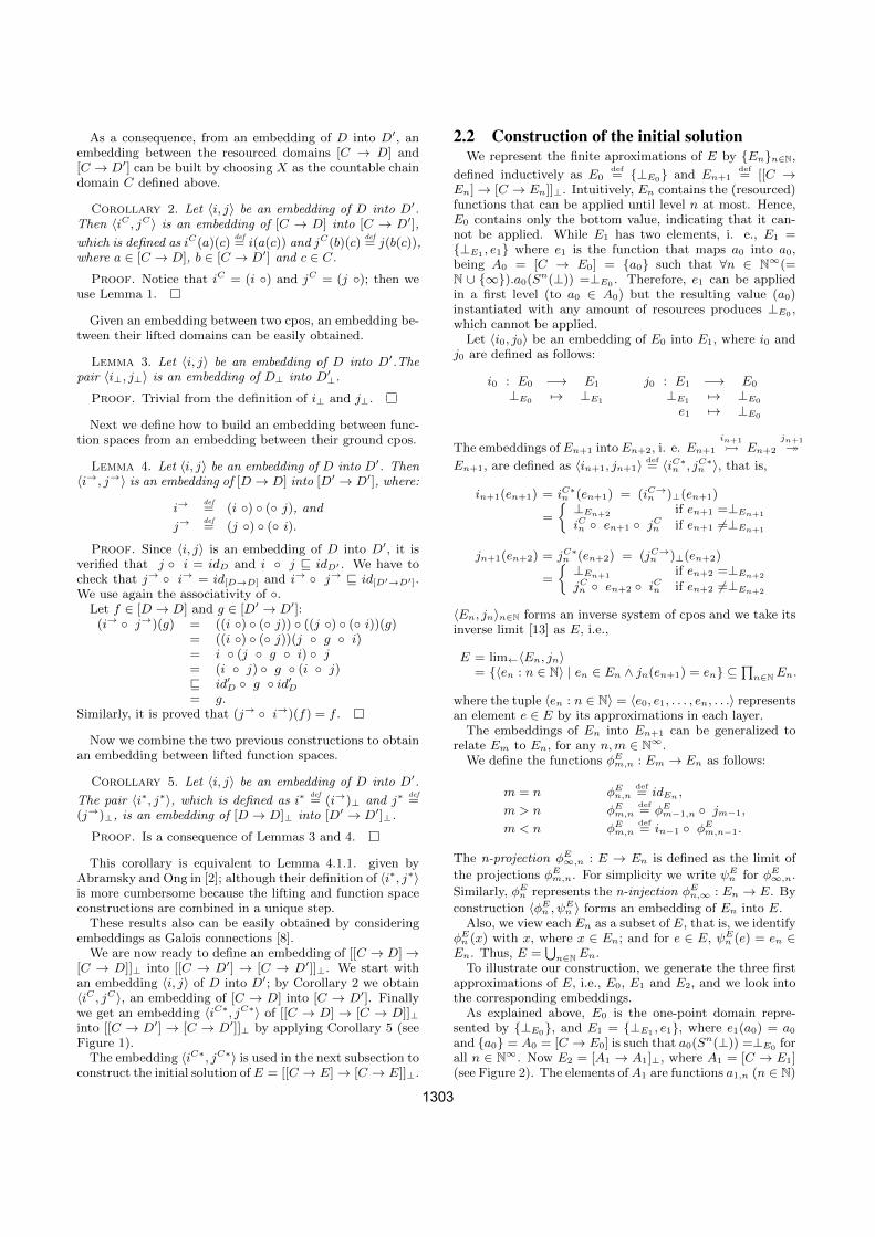
As a consequence, from an embedding of D into D′, anembedding between the resourced domains [C → D] and[C → D′] can be built by choosing X as the countable chaindomain C defined above.
Corollary 2. Let 〈i, j〉 be an embedding of D into D′.Then 〈iC , jC〉 is an embedding of [C → D] into [C → D′],
which is defined as iC(a)(c)def= i(a(c)) and jC(b)(c)
def= j(b(c)),
where a ∈ [C → D], b ∈ [C → D′] and c ∈ C.
Proof. Notice that iC = (i ◦) and jC = (j ◦); then weuse Lemma 1.
Given an embedding between two cpos, an embedding be-tween their lifted domains can be easily obtained.
Lemma 3. Let 〈i, j〉 be an embedding of D into D′.Thepair 〈i⊥, j⊥〉 is an embedding of D⊥ into D′⊥.
Proof. Trivial from the definition of i⊥ and j⊥.
Next we define how to build an embedding between func-tion spaces from an embedding between their ground cpos.
Lemma 4. Let 〈i, j〉 be an embedding of D into D′. Then〈i→, j→〉 is an embedding of [D → D] into [D′ → D′], where:
i→def= (i ◦) ◦ (◦ j), and
j→def= (j ◦) ◦ (◦ i).
Proof. Since 〈i, j〉 is an embedding of D into D′, it isverified that j ◦ i = idD and i ◦ j ⊑ idD′ . We have tocheck that j→ ◦ i→ = id[D→D] and i
→ ◦ j→ ⊑ id[D′→D′].We use again the associativity of ◦.Let f ∈ [D → D] and g ∈ [D′ → D′]:(i→ ◦ j→)(g) = ((i ◦) ◦ (◦ j)) ◦ ((j ◦) ◦ (◦ i))(g)
= ((i ◦) ◦ (◦ j))(j ◦ g ◦ i)= i ◦ (j ◦ g ◦ i) ◦ j= (i ◦ j) ◦ g ◦ (i ◦ j)⊑ id′D ◦ g ◦ id′D= g.
Similarly, it is proved that (j→ ◦ i→)(f) = f .
Now we combine the two previous constructions to obtainan embedding between lifted function spaces.
Corollary 5. Let 〈i, j〉 be an embedding of D into D′.
The pair 〈i∗, j∗〉, which is defined as i∗def= (i→)⊥ and j∗
def=
(j→)⊥, is an embedding of [D → D]⊥ into [D′ → D′]⊥.
Proof. Is a consequence of Lemmas 3 and 4.
This corollary is equivalent to Lemma 4.1.1. given byAbramsky and Ong in [2]; although their definition of 〈i∗, j∗〉is more cumbersome because the lifting and function spaceconstructions are combined in a unique step.These results also can be easily obtained by considering
embeddings as Galois connections [8].We are now ready to define an embedding of [[C → D] →
[C → D]]⊥ into [[C → D′] → [C → D′]]⊥. We start withan embedding 〈i, j〉 of D into D′; by Corollary 2 we obtain〈iC , jC〉, an embedding of [C → D] into [C → D′]. Finallywe get an embedding 〈iC∗, jC∗〉 of [[C → D] → [C → D]]⊥into [[C → D′] → [C → D′]]⊥ by applying Corollary 5 (seeFigure 1).The embedding 〈iC∗, jC∗〉 is used in the next subsection to
construct the initial solution of E = [[C → E] → [C → E]]⊥.
2.2 Construction of the initial solutionWe represent the finite aproximations of E by {En}n∈N,
defined inductively as E0def= {⊥E0} and En+1
def= [[C →
En] → [C → En]]⊥. Intuitively, En contains the (resourced)functions that can be applied until level n at most. Hence,E0 contains only the bottom value, indicating that it can-not be applied. While E1 has two elements, i. e., E1 ={⊥E1 , e1} where e1 is the function that maps a0 into a0,being A0 = [C → E0] = {a0} such that ∀n ∈ N∞(=N ∪ {∞}).a0(S
n(⊥)) =⊥E0 . Therefore, e1 can be appliedin a first level (to a0 ∈ A0) but the resulting value (a0)instantiated with any amount of resources produces ⊥E0 ,which cannot be applied.
Let 〈i0, j0〉 be an embedding of E0 into E1, where i0 andj0 are defined as follows:
i0 : E0 −→ E1 j0 : E1 −→ E0
⊥E0 7→ ⊥E1 ⊥E1 7→ ⊥E0
e1 7→ ⊥E0
The embeddings of En+1 into En+2, i. e. En+1
in+1 En+2
jn+1։En+1, are defined as 〈in+1, jn+1〉 def
= 〈iC∗n , jC∗n 〉, that is,
in+1(en+1) = iC∗n (en+1) = (iC→n )⊥(en+1)
=
{ ⊥En+2 if en+1 =⊥En+1
iCn ◦ en+1 ◦ jCn if en+1 6=⊥En+1
jn+1(en+2) = jC∗n (en+2) = (jC→n )⊥(en+2)
=
{ ⊥En+1 if en+2 =⊥En+2
jCn ◦ en+2 ◦ iCn if en+2 6=⊥En+2
〈En, jn〉n∈N forms an inverse system of cpos and we take itsinverse limit [13] as E, i.e.,
E = lim←〈En, jn〉= {〈en : n ∈ N〉 | en ∈ En ∧ jn(en+1) = en} ⊆ ∏
n∈N En.
where the tuple 〈en : n ∈ N〉 = 〈e0, e1, . . . , en, . . .〉 representsan element e ∈ E by its approximations in each layer.
The embeddings of En into En+1 can be generalized torelate Em to En, for any n,m ∈ N∞.
We define the functions φEm,n : Em → En as follows:
m = n φEn,n
def= idEn ,
m > n φEm,n
def= φE
m−1,n ◦ jm−1,
m < n φEm,n
def= in−1 ◦ φE
m,n−1.
The n-projection φE∞,n : E → En is defined as the limit of
the projections φEm,n. For simplicity we write ψE
n for φE∞,n.
Similarly, φEn represents the n-injection φE
n,∞ : En → E. By
construction 〈φEn , ψ
En 〉 forms an embedding of En into E.
Also, we view each En as a subset of E, that is, we identifyφEn (x) with x, where x ∈ En; and for e ∈ E, ψE
n (e) = en ∈En. Thus, E =
⋃n∈N En.
To illustrate our construction, we generate the three firstapproximations of E, i.e., E0, E1 and E2, and we look intothe corresponding embeddings.
As explained above, E0 is the one-point domain repre-sented by {⊥E0}, and E1 = {⊥E1 , e1}, where e1(a0) = a0
and {a0} = A0 = [C → E0] is such that a0(Sn(⊥)) =⊥E0 for
all n ∈ N∞. Now E2 = [A1 → A1]⊥, where A1 = [C → E1](see Figure 2). The elements of A1 are functions a1,n (n ∈ N)
1303

[C → D]
[C → D]
[C → D′]
[C → D′]
f giC
jC
iC
jC
jC∗
⊥ ⊥iC∗
Figure 1: Embeddings on resourced domains
C
S∞(⊥C )
. . .
Sn(⊥C )
. . .
S(⊥C )
⊥C
e1
⊥E1
C
S∞(⊥C )
. . .
Sn(⊥C )
. . .
S(⊥C )
⊥C
e1
⊥E1
E2A1 A1
E1 E1
⊥E2
Figure 2: The domain E2
such that:
a1,n(Sk(⊥)) =
{⊥E1 if k < ne1 if k ≥ n
We define a1,∞ as the function verifying that forall n ∈ N∞a1,∞(Sn(⊥)) =⊥E1 , i.e., this is the least defined function inA1. Notice that the most defined one is a1,0, the constantfunction with a1,0(S
n(⊥)) = e1 forall n ∈ N∞. Hence, wehave an ordering in A1 where a1,∞ ⊑ a1,m ⊑ a1,n ⊑ a1,0 forall m,n ∈ N such that n ≤ m.Since A1 = {a1,n | n ∈ N∞}, any increasing ω-chain in
A1 has as l.u.b. a1,k for some k ∈ N, except for the con-stant chain {xn = a1,∞}n∈N. Hence, we can characterizethe continuous functions e : A1 → A1 as those that satisfythe following property:
n ≤ m⇒ l ≤ k, for e(a1,m) = a1,k and e(a1,n) = a1,l (1)
Summarizing,
E2 = {⊥E2} ∪ {e : {a1,n}n∈N∞ → {a1,n}n∈N∞ | e sat.(1)}.The representation of the embeddings 〈i0, j0〉 of E0 into E1
and 〈i1, j1〉 of E1 into E2 is shown in Figure 3. For E2 weonly highlight the constant functions e2,∞ and e2,0 repre-senting the two extremes of [A1 → A1], i.e., for all n ∈ N∞
e2,∞(a1,n) = a1,∞ and e2,0(a1,n) = a1,0.
2.3 Application operationsApplication operations are defined in each domain En as
Ap⊥En: En+1 ×An × C → En,
Ap⊥En(en+1, an, c)
def=
{⊥En if en+1 =⊥En+1
en+1(an)(c) if en+1 6=⊥En+1
ψEn denotes the n-projection defined in Section 2.2 for the
domain E. From the embedding 〈φEn , ψ
En 〉 of En into E and
using Corollary 2, we obtain the embedding 〈(φEn )
C , (ψEn )C〉
of [C → En] into [C → E], so that ψ[C→E]n stands for (ψE
n )C .Application operation in E is AP⊥E : E× [C → E]×C → E,
AP⊥E (e, a, c)def=
⊔
n∈NAp⊥En
(ψEn+1(e), ψ
[C→E]n (a), c).
In the following, we use e(a)(c) for both Ap⊥En(e, a, c) and
AP ⊥E (e, a, c); from the context it should be clear which isthe correct one. Notice that
ψEn (e(a)(c)) = ψE
n+1(e)(ψ[C→E]n (a))(c). (2)
Analogously, from the definition of the application opera-tion in the standard lifted function space D described in [2],
where D is the initial solution of D = [D → D]⊥ and thisinitial solution can be described as an inverse limit similarlyto E, it can be observed that
ψDn (d(d′)) = ψD
n+1(d)(ψDn (d′)). (3)
3. SIMILARITYIn this section we define a relation between the standard
lifted function domain D = [D → D]⊥ and the resourceddomain E = [[C → E] → [C → E]]⊥ constructed in theprevious section. Our relation is inspired by the applicativebisimulation defined by Abramsky in [1], so that functionsd ∈ D and e ∈ E are considered to be similar if d and ehave a similar applicative behaviour when infinite resourcesare available for e, i.e., they produce similar values whenapplied to similar arguments.
To formalize this circular definition we resort to a layeredconstruction, that is, we inductively define a sequence ofrelations { ⊳⊲n ⊆ Dn × En}n∈N.
Definition 1 (n-similarity). A family of n-similarityrelations between elements of Dn and En, for n ∈ N, is de-fined as follows:
• 0-similarity, ⊳⊲0 : ⊥D0 ⊳⊲0 ⊥E0 .
• n+1-similarity, ⊳⊲n+1 , is the least relation in Dn+1×En+1 that verifies:(1) ⊥Dn+1 ⊳⊲n+1 ⊥En+1 and,(2) let d ∈ Dn+1 and e ∈ En+1 such that d 6=⊥Dn+1
and e 6=⊥En+1 , then d ⊳⊲n+1 e if for any d′ ∈ Dn andfor any a′ ∈ An, d
′ ⊳⊲n a′(S∞) ⇒ d(d′) ⊳⊲n e(a
′)(S∞).
For a better understanding of this definition, we show thethree first layers (Figure 4):
• 0-similarity (⊳⊲0): D0 = {⊥D0} and E0 = {⊥E0}, so thatthe relation reduces to ⊥D0 ⊳⊲0 ⊥E0 .
• 1-similarity (⊳⊲1 ): D1 = {⊥D1 , d1}, where d1 ∈ [D0 →D0] is the function mapping ⊥D0 into ⊥D0 , and recall thatE1 = {⊥E1 , e1} with e1(a0) = a0. ⊥D1 ⊳⊲1 ⊥E1 , bydefinition. Now let d′ ∈ D0 and a′ ∈ A0 = {a0 | ∀n ∈N∞. a0(S
n(⊥)) =⊥E0}, it must be that d′ =⊥D0 and a′ =a0. Hence, we have that ⊥D0= d′ ⊳⊲0 a′(S∞) =⊥E0 . More-over, d1(d
′) =⊥D0 ⊳⊲0 ⊥E0= a0(S∞) = e1(a0)(S
∞) =e1(a
′)(S∞). Thus, d1 ⊳⊲1 e1.
• 2-similarity (⊳⊲2): D2 = {⊥D2 , d2,1, d2,2, d2,3}, where thefunctions d2,1, d2,2 and d2,3 are defined as follows:
d2,1(⊥D1) = ⊥D1 d2,2(⊥D1) = ⊥D1 d2,3(⊥D1) = d1
d2,1(d1) = ⊥D1 d2,2(d1) = d1 d2,3(d1) = d1
1304
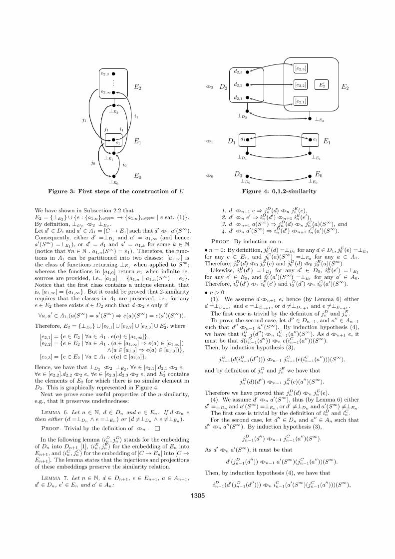
...
i0j0
i1
i1j1
j1
E0
E1
E2
⊥E0
⊥E1
⊥E2
e1
e2,∞
e2,0
Figure 3: First steps of the construction of E
E0
E1
E2
⊥E0
⊥E1
⊥E2
e1
[e2,1]
[e2,2]
[e2,3]
E′2
D0
D1
D2
⊥D0
⊥D1
⊥D2
d1
d2,1
d2,2
d2,3
⊳⊲0
⊳⊲1
⊳⊲2
Figure 4: 0,1,2-similarity
We have shown in Subsection 2.2 thatE2 = {⊥E2} ∪ {e : {a1,n}n∈N∞ → {a1,n}n∈N∞ | e sat. (1)}.By definition, ⊥D2 ⊳⊲2 ⊥E2 .Let d′ ∈ D1 and a
′ ∈ A1 = [C → E1] such that d′ ⊳⊲1 a′(S∞).
Consequently, either d′ =⊥D1 and a′ = a1,∞ (and hencea′(S∞) =⊥E1), or d
′ = d1 and a′ = a1,k for some k ∈ N(notice that ∀n ∈ N . a1,n(S
∞) = e1). Therefore, the func-tions in A1 can be partitioned into two classes: [a1,∞] isthe class of functions returning ⊥E1 when applied to S∞;whereas the functions in [a1,0] return e1 when infinite re-sources are provided, i.e., [a1,0] = {a1,n | a1,n(S
∞) = e1}.Notice that the first class contains a unique element, thatis, [a1,∞] = {a1,∞}. But it could be proved that 2-similarityrequires that the classes in A1 are preserved, i.e., for anye ∈ E2 there exists d ∈ D2 such that d ⊳⊲2 e only if
∀a, a′ ∈ A1.(a(S∞) = a′(S∞) ⇒ e(a)(S∞) = e(a′)(S∞)).
Therefore, E2 = {⊥E2} ∪ [e2,1] ∪ [e2,2] ∪ [e2,3] ∪ E′2. where[e2,1] = {e ∈ E2 | ∀a ∈ A1 . e(a) ∈ [a1,∞]},[e2,2] = {e ∈ E2 | ∀a ∈ A1 . (a ∈ [a1,∞] ⇒ e(a) ∈ [a1,∞])
∧(a ∈ [a1,0] ⇒ e(a) ∈ [a1,0])},[e2,3] = {e ∈ E2 | ∀a ∈ A1 . e(a) ∈ [a1,0]}.
Hence, we have that ⊥D2 ⊳⊲2 ⊥E2 , ∀e ∈ [e2,1].d2,1 ⊳⊲2 e,∀e ∈ [e2,2].d2,2 ⊳⊲2 e, ∀e ∈ [e2,3].d2,3 ⊳⊲2 e, and E
′2 contains
the elements of E2 for which there is no similar element inD2. This is graphically represented in Figure 4.Next we prove some useful properties of the n-similarity,
e.g., that it preserves undefinedness:
Lemma 6. Let n ∈ N, d ∈ Dn and e ∈ En. If d ⊳⊲n ethen either (d =⊥Dn ∧ e =⊥En) or (d 6=⊥Dn ∧ e 6=⊥En).
Proof. Trivial by the definition of ⊳⊲n .
In the following lemma 〈iDn , jDn 〉 stands for the embeddingof Dn into Dn+1 [1], 〈iEn , jEn 〉 for the embedding of En intoEn+1, and 〈iCn , jCn 〉 for the embedding of [C → En] into [C →En+1]. The lemma states that the injections and projectionsof these embeddings preserve the similarity relation.
Lemma 7. Let n ∈ N, d ∈ Dn+1, e ∈ En+1, a ∈ An+1,d′ ∈ Dn, e′ ∈ En and a′ ∈ An:
1. d ⊳⊲n+1 e⇒ jDn (d) ⊳⊲n jEn (e),
2. d′ ⊳⊲n e′ ⇒ iDn (d′) ⊳⊲n+1 i
En (e′),
3. d ⊳⊲n+1 a(S∞) ⇒ jDn (d) ⊳⊲n j
Cn (a)(S∞), and
4. d′ ⊳⊲n a′(S∞) ⇒ iDn (d′) ⊳⊲n+1 i
Cn (a
′)(S∞).
Proof. By induction on n.
• n = 0: By definition, jD0 (d) =⊥D0 for any d ∈ D1, jE0 (e) =⊥E1
for any e ∈ E1, and jC0 (a)(S∞) =⊥E0 for any a ∈ A1.Therefore, jD0 (d) ⊳⊲0 j
E0 (e) and jD0 (d) ⊳⊲0 j
E0 (a)(S∞).
Likewise, iD0 (d′) =⊥D1 for any d′ ∈ D0, iE0 (e′) =⊥E1
for any e′ ∈ E0, and iC0 (a′)(S∞) =⊥E1 for any a′ ∈ A0.
Therefore, iD0 (d′) ⊳⊲1 iE0 (e′) and iD0 (d′) ⊳⊲1 i
C0 (a
′)(S∞).
• n > 0:(1). We assume d ⊳⊲n+1 e, hence (by Lemma 6) either
d =⊥Dn+1 and e =⊥En+1 , or d 6=⊥Dn+1 and e 6=⊥En+1 .
The first case is trivial by the definiton of jDn and jEn .To prove the second case, let d′′ ∈ Dn−1, and a
′′ ∈ An−1
such that d′′ ⊳⊲n−1 a′′(S∞). By induction hypothesis (4),
we have that iDn−1(d′′) ⊳⊲n iCn−1(a
′′)(S∞). As d ⊳⊲n+1 e, itmust be that d(iDn−1(d
′′)) ⊳⊲n e(iCn−1(a
′′))(S∞).Then, by induction hypothesis (3),
jDn−1(d(iDn−1(d
′′))) ⊳⊲n−1 jCn−1(e(i
Cn−1(a
′′)))(S∞),
and by definition of jDn and jEn we have that
jDn (d)(d′′) ⊳⊲n−1 jEn (e)(a′′)(S∞).
Therefore we have proved that jDn (d) ⊳⊲n jEn (e).
(4). We assume d′ ⊳⊲n a′(S∞), thus (by Lemma 6) either
d′ =⊥Dn and a′(S∞) =⊥En , or d′ 6=⊥Dn and a′(S∞) 6=⊥En .
The first case is trivial by the definition of iDn and iCn .For the second case, let d′′ ∈ Dn and a′′ ∈ An such that
d′′ ⊳⊲n a′′(S∞). By induction hypothesis (3),
jDn−1(d′′) ⊳⊲n−1 j
Cn−1(a
′′)(S∞).
As d′ ⊳⊲n a′(S∞), it must be that
d′(jDn−1(d′′)) ⊳⊲n−1 a
′(S∞)(jCn−1(a′′))(S∞).
Then, by induction hypothesis (4), we have that
iDn−1(d′(jDn−1(d
′′))) ⊳⊲n iCn−1(a
′(S∞)(jCn−1(a′′)))(S∞),
1305
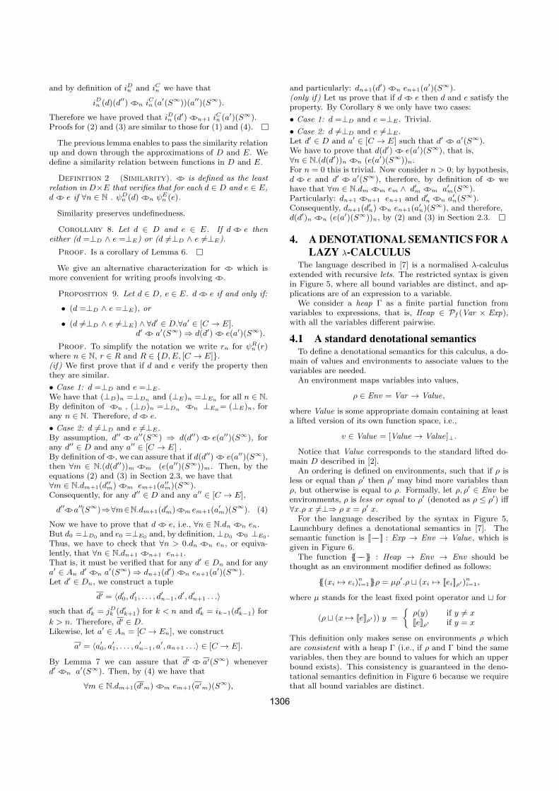
and by definition of iDn and iCn we have that
iDn (d)(d′′) ⊳⊲n iCn (a
′(S∞))(a′′)(S∞).
Therefore we have proved that iDn (d′) ⊳⊲n+1 iCn (a
′)(S∞).Proofs for (2) and (3) are similar to those for (1) and (4).
The previous lemma enables to pass the similarity relationup and down through the approximations of D and E. Wedefine a similarity relation between functions in D and E.
Definition 2 (Similarity). ⊳⊲ is defined as the leastrelation in D×E that verifies that for each d ∈ D and e ∈ E,d ⊳⊲ e if ∀n ∈ N . ψD
n (d) ⊳⊲n ψEn (e).
Similarity preserves undefinedness.
Corollary 8. Let d ∈ D and e ∈ E. If d ⊳⊲ e theneither (d =⊥D ∧ e =⊥E) or (d 6=⊥D ∧ e 6=⊥E).
Proof. Is a corollary of Lemma 6.
We give an alternative characterization for ⊳⊲ which ismore convenient for writing proofs involving ⊳⊲.
Proposition 9. Let d ∈ D, e ∈ E. d ⊳⊲ e if and only if:
• (d =⊥D ∧ e =⊥E), or
• (d 6=⊥D ∧ e 6=⊥E) ∧ ∀d′ ∈ D.∀a′ ∈ [C → E].d′ ⊳⊲ a′(S∞) ⇒ d(d′) ⊳⊲ e(a′)(S∞).
Proof. To simplify the notation we write rn for ψRn (r)
where n ∈ N, r ∈ R and R ∈ {D,E, [C → E]}.(if) We first prove that if d and e verify the property thenthey are similar.
• Case 1: d =⊥D and e =⊥E .We have that (⊥D)n =⊥Dn and (⊥E)n =⊥En for all n ∈ N.By definiton of ⊳⊲n , (⊥D)n =⊥Dn ⊳⊲n ⊥En= (⊥E)n, forany n ∈ N. Therefore, d ⊳⊲ e.• Case 2: d 6=⊥D and e 6=⊥E .By assumption, d′′ ⊳⊲ a′′(S∞) ⇒ d(d′′) ⊳⊲ e(a′′)(S∞), forany d′′ ∈ D and any a′′ ∈ [C → E] .By definition of ⊳⊲, we can assure that if d(d′′) ⊳⊲ e(a′′)(S∞),then ∀m ∈ N.(d(d′′))m ⊳⊲m (e(a′′)(S∞))m. Then, by theequations (2) and (3) in Section 2.3, we have that∀m ∈ N.dm+1(d
′′m) ⊳⊲m em+1(a
′′m)(S∞).
Consequently, for any d′′ ∈ D and any a′′ ∈ [C → E],
d′′⊳⊲a′′(S∞)⇒∀m∈N.dm+1(d′m)⊳⊲m em+1(a
′m)(S∞). (4)
Now we have to prove that d ⊳⊲ e, i.e., ∀n ∈ N.dn ⊳⊲n en.But d0 =⊥D0 and e0 =⊥E0 and, by definition, ⊥D0 ⊳⊲0 ⊥E0 .Thus, we have to check that ∀n > 0.dn ⊳⊲n en, or equiva-lently, that ∀n ∈ N.dn+1 ⊳⊲n+1 en+1.That is, it must be verified that for any d′ ∈ Dn and for anya′ ∈ An d
′ ⊳⊲n a′(S∞) ⇒ dn+1(d
′) ⊳⊲n en+1(a′)(S∞).
Let d′ ∈ Dn, we construct a tuple
d′ = 〈d′0, d′1, . . . , d′n−1, d′, d′n+1 . . .〉
such that d′k = jDk (d′k+1) for k < n and d′k = ik−1(d′k−1) for
k > n. Therefore, d′ ∈ D.Likewise, let a′ ∈ An = [C → En], we construct
a′ = 〈a′0, a′1, . . . , a′n−1, a′, an+1 . . .〉 ∈ [C → E].
By Lemma 7 we can assure that d′ ⊳⊲ a′(S∞) wheneverd′ ⊳⊲n a′(S∞). Then, by (4) we have that
∀m ∈ N.dm+1(d′m) ⊳⊲m em+1(a′m)(S∞),
and particularly: dn+1(d′) ⊳⊲n en+1(a
′)(S∞).(only if) Let us prove that if d ⊳⊲ e then d and e satisfy theproperty. By Corollary 8 we only have two cases:
• Case 1: d =⊥D and e =⊥E . Trivial.
• Case 2: d 6=⊥D and e 6=⊥E .Let d′ ∈ D and a′ ∈ [C → E] such that d′ ⊳⊲ a′(S∞).We have to prove that d(d′) ⊳⊲ e(a′)(S∞), that is,∀n ∈ N.(d(d′))n ⊳⊲n (e(a′)(S∞))n.For n = 0 this is trivial. Now consider n > 0; by hypothesis,d ⊳⊲ e and d′ ⊳⊲ a′(S∞), therefore, by definition of ⊳⊲ wehave that ∀m ∈ N.dm ⊳⊲m em ∧ d′m ⊳⊲m a′m(S∞).Particularly: dn+1 ⊳⊲n+1 en+1 and d′n ⊳⊲n a
′n(S
∞).Consequently, dn+1(d
′n) ⊳⊲n en+1(a
′n)(S
∞), and therefore,d(d′)n ⊳⊲n (e(a′)(S∞))n, by (2) and (3) in Section 2.3.
4. A DENOTATIONAL SEMANTICS FOR ALAZY λ-CALCULUS
The language described in [7] is a normalised λ-calculusextended with recursive lets. The restricted syntax is givenin Figure 5, where all bound variables are distinct, and ap-plications are of an expression to a variable.
We consider a heap Γ as a finite partial function fromvariables to expressions, that is, Heap ∈ Pf (Var × Exp),with all the variables different pairwise.
4.1 A standard denotational semanticsTo define a denotational semantics for this calculus, a do-
main of values and environments to associate values to thevariables are needed.
An environment maps variables into values,
ρ ∈ Env = Var → Value,
where Value is some appropriate domain containing at leasta lifted version of its own function space, i.e.,
v ∈ Value = [Value → Value]⊥.
Notice that Value corresponds to the standard lifted do-main D described in [2].
An ordering is defined on environments, such that if ρ isless or equal than ρ′ then ρ′ may bind more variables thanρ, but otherwise is equal to ρ. Formally, let ρ, ρ′ ∈ Env beenvironments, ρ is less or equal to ρ′ (denoted as ρ ≤ ρ′) iff∀x.ρ x 6=⊥⇒ ρ x = ρ′ x.
For the language described by the syntax in Figure 5,Launchbury defines a denotational semantics in [7]. Thesemantic function is [[−−]] : Exp → Env → Value, which isgiven in Figure 6.
The function {{−−}} : Heap → Env → Env should bethought as an environment modifier defined as follows:
{{(xi 7→ ei)ni=1}}ρ = µρ′.ρ ⊔ (xi 7→ [[ei]]ρ′)
ni=1,
where µ stands for the least fixed point operator and ⊔ for
(ρ ⊔ (x 7→ [[e]]ρ′)) y =
{ρ(y) if y 6= x[[e]]ρ′ if y = x
This definition only makes sense on environments ρ whichare consistent with a heap Γ (i.e., if ρ and Γ bind the samevariables, then they are bound to values for which an upperbound exists). This consistency is guaranteed in the deno-tational semantics definition in Figure 6 because we requirethat all bound variables are distinct.
1306

x ∈ Vare ∈ Exp ::= x
| λx.e| e x| let {xi = ei}ni=1 in e
Figure 5: Syntax
[[x]]ρ = ρ x[[λx.e]]ρ = up(λν.[[e]]ρ⊔{x 7→ν})[[e x]]ρ = AP⊥D ([[e]]ρ, [[x]]ρ)
[[let {xi = ei}ni=1 in e]]ρ = [[e]]{{(xi 7→ei)ni=1}}ρ
Figure 6: Denotational Semantics
4.2 A resourced denotational semanticsA resourced denotational semantics is also defined in [7],
where the meaning of an expression depends on the numberof available resources. For this a new domain of values, andthe corresponding environments, are needed.A resourced environment is a function mapping variables
into functions from resources to values,
σ ∈ CEnv = Var → [C → CValue],
where CValue is some appropiate resourced domain, i.e.,
CValue = [[C → CValue] → [C → CValue]]⊥.
Notice that CValue corresponds to the resourced domainE constructed in Section 2.An ordering is defined on resourced environments too,
such that if σ is less or equal than σ′ then, for any num-ber of available resources, σ′ may bind more variables thanσ, but otherwise is equal to σ: Let σ, σ′ ∈ CEnv be re-sourced environments, σ is less or equal than σ′ (denoted asσ ≤ σ′) iff ∀x ∈ Var and ∀m ∈ N
σx(Sm(⊥)) 6=⊥⇒ σ x(Sm(⊥)) = σ′x(Sm(⊥)).
The resourced semantics focuses on approximations to thesemantics of Figure 6. The semantic function N [[−−]] :Exp → CEnv → [C → CValue] is given in Figure 7.The function N{{−−}} : Heap → CEnv → CEnv is defined
analogously to {{−}}:N{{(xi 7→ Ei)
ni=1}}σ = µσ′.σ ⊔ (xi 7→ N [[Ei]]σ′ )ni=1.
4.3 EquivalenceIn Section 3 we have shown how to relate values in Value
with values in CValue, but we need to extend the notion ofsimilarity to environments:
Definition 3. (Similarity of environments). Let ρ ∈ Envbe an environment and σ ∈ CEnv be a resourced environ-ment. ρ and σ are similar (denoted by ρ ⊳⊲ σ) when
∀x ∈ Var .ρ x ⊳⊲ σ x(S∞).
Now we can prove the equivalence between the standarddenotational semantics and the resourced one. More pre-cisely, we prove that they produce similar values.
Theorem 10. Let e ∈ Exp be an expression and ρ ∈ Env,σ ∈ CEnv be similar environments (i.e., ρ ⊳⊲ σ), then
[[e]]ρ ⊳⊲ N [[e]]σ (S∞).
Proof. By structural induction on e:
e ≡ x
By definition, [[x]]ρ = ρ x and N [[x]]σ (S∞) = σ x(S∞).By hypothesis ρ ⊳⊲ σ, therefore:[[x]]ρ = ρ x ⊳⊲ σ x(S∞) = N [[x]]σ (S∞).
e ≡ λx.e′
By definition, [[λx.e′]]ρ = up(λν.[[e′]]ρ⊔{x 7→ν}) 6=⊥Value andN [[λx.e′]]σ (S∞) = up(λτ.N [[e′]]σ⊔{x 7→τ} ) 6=⊥CValue .We have to prove thatup(λν.[[e′]]ρ⊔{x 7→ν}) ⊳⊲ up(λτ.N [[e′]]σ⊔{x 7→τ} ).We use the alternative characterization of similarity (Propo-sition 9). Let v ∈ Value and f ∈ C → CValue such thatv ⊳⊲ f(S∞), then:AP⊥D (up(λν.[[e′]]ρ⊔{x 7→ν}), v) = [[e′]]ρ⊔{x 7→v} and
AP⊥E (up(λτ.N [[e′]]σ⊔{x 7→τ} ), f, S∞) = N [[e′]]σ⊔{x 7→f} (S
∞).If ρ′ = ρ ⊔ {x 7→ v} ⊳⊲ σ ⊔ {x 7→ f} = σ′, then, by induc-tion hypothesis, we get the desired result.Let us prove that ρ′ ⊳⊲ σ′:
• If y 6= x then ρ′ y = ρ y ⊳⊲ σ y(S∞) = σ′ y, because ρ ⊳⊲ σ.
• If y = x then ρ′ y = v ⊳⊲ f(S∞) = σ′ y, by hypothesis.
Thus, [[e′]]ρ′ ⊳⊲ N [[e′]]σ′ (S∞).Therefore, we have proved that [[λx.e′]]ρ ⊳⊲ N [[λx.e′]]σ (S∞).
e ≡ e′ x
By definition, [[e′ x]]ρ = AP⊥D ([[e′]]ρ, [[x]]ρ) andN [[e′ x]]σ (S∞) = AP⊥E (N [[e′]]σ S
∞,N [[x]]σ , S∞).
Thus, we have to prove thatAP⊥D ([[e′]]ρ, [[x]]ρ) ⊳⊲ AP⊥E (N [[e′]]σ (S∞),N [[x]]σ , S
∞).By induction hypothesis, [[e′]]ρ ⊳⊲ N [[e′]]σ (S∞). Then byCorollary 8 there are two cases:• Case 1: [[e′]]ρ =⊥Value and N [[e′]]σ (S∞) =⊥CValue .
[[e′ x]]ρ = AP⊥D ([[e′]]ρ, [[x]]ρ) = AP⊥D (⊥Value , [[x]]ρ) = ⊥Value
⊳⊲ ⊥CValue = AP⊥E (⊥CValue ,N [[x]]σ , S∞)
= AP⊥E (N [[e′]]σ (S∞),N [[x]]σ , S∞) = N [[e′ x]]σ (S∞).
• Case 2: ⊥Value 6= [[e′]]ρ ⊳⊲ N [[e′]]σ (S∞) 6=⊥CValue .Thus, AP⊥D ([[e′]]ρ, [[x]]ρ) = [[e′]]ρ([[x]]ρ) andAP⊥E (N [[e′]]σ (S∞),N [[x]]σ , S
∞) =N [[e′]]σ (S∞)(N [[x]]σ ) (S
∞).By induction hypothesis [[x]]ρ ⊳⊲ N [[x]]σ (S∞).Therefore, by the alternative characterization for ⊳⊲ :[[e′]]ρ([[x]]ρ) ⊳⊲ N [[e′]]σ (S∞)(N [[x]]σ ) (S∞).So that [[e′ x]]ρ ⊳⊲ N [[e′x]]σ (S∞).
e ≡ let {xi = ei}ni=1 in e′
By definition:[[let {xi = ei}ni=1 in e′]]ρ = [[e′]]{{(xi 7→ei)
ni=1}}ρ and
N [[let {xi = ei}ni=1 in e′]]σ (S∞) =N [[e′]]N{{(xi 7→ei)
ni=1}}σ (S∞).
Using fix point techniques it can be proved that if ρ ⊳⊲ σthen {{Γ}}ρ ⊳⊲ N{{Γ}}σ for any heap Γ consistent with ρ andσ. Thus, {{(xi 7→ ei)
ni=1}}ρ ⊳⊲ N{{(xi 7→ ei)
ni=1}}σ.
By induction hypothesis:[[e′]]{{(xi 7→ei)
ni=1}}ρ ⊳⊲ N [[e′]]N{{(xi 7→ei)
ni=1}}σ (S∞).
Therefore, we obtain that[[let {xi = ei}ni=1 in e′]]ρ ⊳⊲
N [[let {xi = ei}ni=1 in e′]]σ (S∞).
This result allows to prove the computational adequacy ofthe natural semantics with respect to the denotational one.
1307
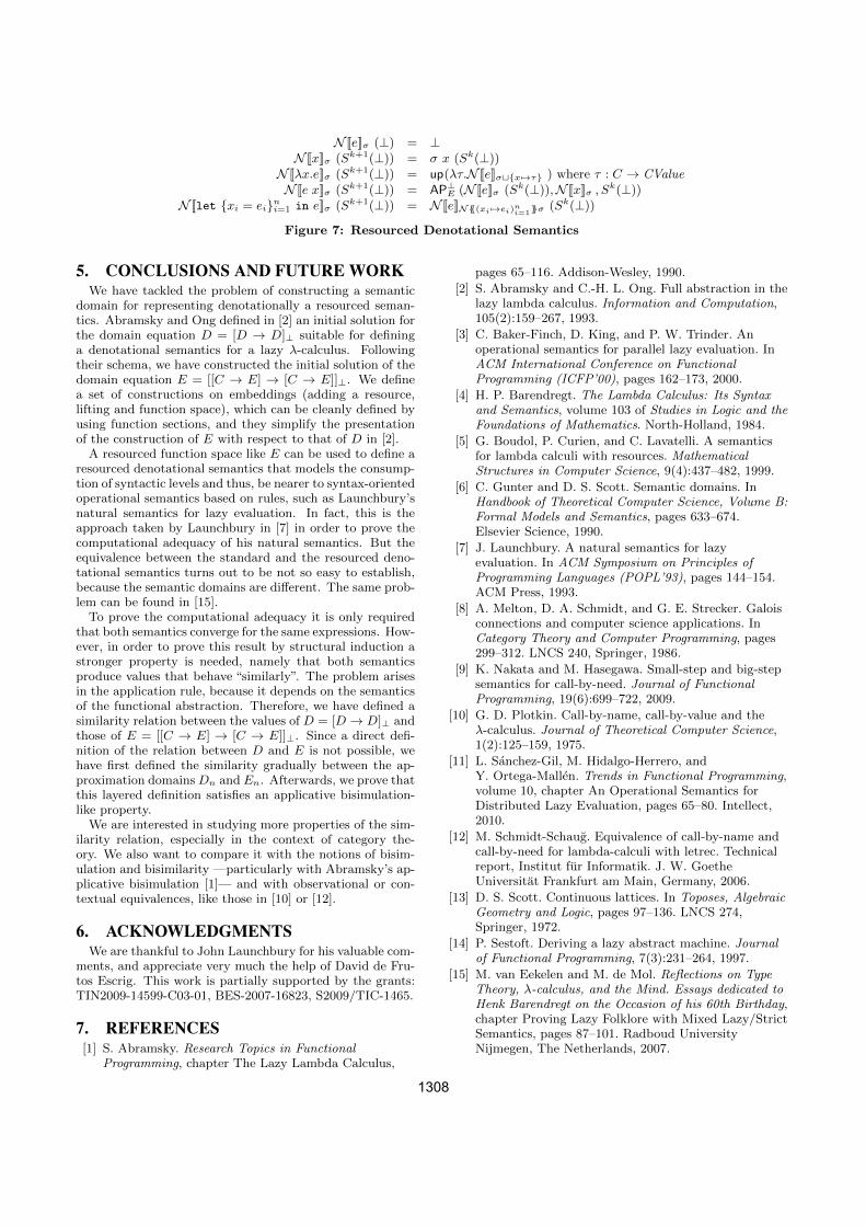
N [[e]]σ (⊥) = ⊥N [[x]]σ (Sk+1(⊥)) = σ x (Sk(⊥))
N [[λx.e]]σ (Sk+1(⊥)) = up(λτ.N [[e]]σ⊔{x 7→τ} ) where τ : C → CValueN [[e x]]σ (Sk+1(⊥)) = AP⊥E (N [[e]]σ (Sk(⊥)),N [[x]]σ , S
k(⊥))N [[let {xi = ei}ni=1 in e]]σ (Sk+1(⊥)) = N [[e]]N{{(xi 7→ei)
ni=1}}σ (Sk(⊥))
Figure 7: Resourced Denotational Semantics
5. CONCLUSIONS AND FUTURE WORKWe have tackled the problem of constructing a semantic
domain for representing denotationally a resourced seman-tics. Abramsky and Ong defined in [2] an initial solution forthe domain equation D = [D → D]⊥ suitable for defininga denotational semantics for a lazy λ-calculus. Followingtheir schema, we have constructed the initial solution of thedomain equation E = [[C → E] → [C → E]]⊥. We definea set of constructions on embeddings (adding a resource,lifting and function space), which can be cleanly defined byusing function sections, and they simplify the presentationof the construction of E with respect to that of D in [2].A resourced function space like E can be used to define a
resourced denotational semantics that models the consump-tion of syntactic levels and thus, be nearer to syntax-orientedoperational semantics based on rules, such as Launchbury’snatural semantics for lazy evaluation. In fact, this is theapproach taken by Launchbury in [7] in order to prove thecomputational adequacy of his natural semantics. But theequivalence between the standard and the resourced deno-tational semantics turns out to be not so easy to establish,because the semantic domains are different. The same prob-lem can be found in [15].To prove the computational adequacy it is only required
that both semantics converge for the same expressions. How-ever, in order to prove this result by structural induction astronger property is needed, namely that both semanticsproduce values that behave “similarly”. The problem arisesin the application rule, because it depends on the semanticsof the functional abstraction. Therefore, we have defined asimilarity relation between the values of D = [D → D]⊥ andthose of E = [[C → E] → [C → E]]⊥. Since a direct defi-nition of the relation between D and E is not possible, wehave first defined the similarity gradually between the ap-proximation domainsDn and En. Afterwards, we prove thatthis layered definition satisfies an applicative bisimulation-like property.We are interested in studying more properties of the sim-
ilarity relation, especially in the context of category the-ory. We also want to compare it with the notions of bisim-ulation and bisimilarity —particularly with Abramsky’s ap-plicative bisimulation [1]— and with observational or con-textual equivalences, like those in [10] or [12].
6. ACKNOWLEDGMENTSWe are thankful to John Launchbury for his valuable com-
ments, and appreciate very much the help of David de Fru-tos Escrig. This work is partially supported by the grants:TIN2009-14599-C03-01, BES-2007-16823, S2009/TIC-1465.
7. REFERENCES[1] S. Abramsky. Research Topics in Functional
Programming, chapter The Lazy Lambda Calculus,
pages 65–116. Addison-Wesley, 1990.
[2] S. Abramsky and C.-H. L. Ong. Full abstraction in thelazy lambda calculus. Information and Computation,105(2):159–267, 1993.
[3] C. Baker-Finch, D. King, and P. W. Trinder. Anoperational semantics for parallel lazy evaluation. InACM International Conference on FunctionalProgramming (ICFP’00), pages 162–173, 2000.
[4] H. P. Barendregt. The Lambda Calculus: Its Syntaxand Semantics, volume 103 of Studies in Logic and theFoundations of Mathematics. North-Holland, 1984.
[5] G. Boudol, P. Curien, and C. Lavatelli. A semanticsfor lambda calculi with resources. MathematicalStructures in Computer Science, 9(4):437–482, 1999.
[6] C. Gunter and D. S. Scott. Semantic domains. InHandbook of Theoretical Computer Science, Volume B:Formal Models and Semantics, pages 633–674.Elsevier Science, 1990.
[7] J. Launchbury. A natural semantics for lazyevaluation. In ACM Symposium on Principles ofProgramming Languages (POPL’93), pages 144–154.ACM Press, 1993.
[8] A. Melton, D. A. Schmidt, and G. E. Strecker. Galoisconnections and computer science applications. InCategory Theory and Computer Programming, pages299–312. LNCS 240, Springer, 1986.
[9] K. Nakata and M. Hasegawa. Small-step and big-stepsemantics for call-by-need. Journal of FunctionalProgramming, 19(6):699–722, 2009.
[10] G. D. Plotkin. Call-by-name, call-by-value and theλ-calculus. Journal of Theoretical Computer Science,1(2):125–159, 1975.
[11] L. Sanchez-Gil, M. Hidalgo-Herrero, andY. Ortega-Mallen. Trends in Functional Programming,volume 10, chapter An Operational Semantics forDistributed Lazy Evaluation, pages 65–80. Intellect,2010.
[12] M. Schmidt-Schaug. Equivalence of call-by-name andcall-by-need for lambda-calculi with letrec. Technicalreport, Institut fur Informatik. J. W. GoetheUniversitat Frankfurt am Main, Germany, 2006.
[13] D. S. Scott. Continuous lattices. In Toposes, AlgebraicGeometry and Logic, pages 97–136. LNCS 274,Springer, 1972.
[14] P. Sestoft. Deriving a lazy abstract machine. Journalof Functional Programming, 7(3):231–264, 1997.
[15] M. van Eekelen and M. de Mol. Reflections on TypeTheory, λ-calculus, and the Mind. Essays dedicated toHenk Barendregt on the Occasion of his 60th Birthday,chapter Proving Lazy Folklore with Mixed Lazy/StrictSemantics, pages 87–101. Radboud UniversityNijmegen, The Netherlands, 2007.
1308

A Locally Nameless Representation
for a Natural Semantics for Lazy Evaluation
Lidia Sanchez-Gil1, Mercedes Hidalgo-Herrero2, and Yolanda Ortega-Mallen1
1 Dpto. Sistemas Informaticos y Computacion, Facultad de CC. Matematicas,Universidad Complutense de Madrid, Spain
2 Dpto. Didactica de las Matematicas, Facultad de Educacion,Universidad Complutense de Madrid, Spain
Abstract. We propose a locally nameless representation for Launch-bury’s natural semantics for lazy evaluation. Names are reserved for freevariables, while bound variable names are replaced by indices. This avoidsthe use of α-conversion and Barendregt’s variable convention, and facil-itates proof formalization. Our definition includes the management ofmulti-binders to represent simultaneous recursive local declarations. Weuse cofinite quantification to express the semantic rules that require theintroduction of fresh names, but we show that existential rules are ad-missible too. Moreover, we prove that the choice of names during theevaluation of a term is irrelevant as long as they are fresh enough.
1 Motivation
Call-by-need evaluation, which avoids repeated computations, is the semanticfoundation for lazy functional programming languages like Haskell or Clean.Launchbury defines in [7] a natural semantics for lazy evaluation where the setof bindings, i.e., (variable, expression) pairs, is explicitly managed to make pos-sible their sharing. In order to prove that this lazy semantics is correct andcomputationally adequate with respect to a standard denotational semantics,Launchbury introduces some variations in his natural semantics. On the onehand, functional application is modeled denotationally by extending the envi-ronment with a variable bound to a value. This new variable represents theformal parameter of the function, while the value corresponds to the actual ar-gument. For a closer approach of this mechanism, applications are carried out inthe alternative semantics by introducing indirections instead of by performingthe β-reduction through substitution. On the other hand, the update of bindingswith their computed values is an operational notion without counterpart in thestandard denotational semantics, so that the alternative natural semantics doesno longer update bindings and becomes a call-by-name semantics.
Unfortunately, the proof of the equivalence between the lazy natural semanticsand its alternative version with indirections and nonupdate is detailed nowhere,and a simple induction turns out to be insufficient. Intuitively, both reductionsystems should produce the same results. However, this cannot be directly estab-lished since final values may contain free variables which are dependent on the
A. Roychoudhury and M. D’Souza (Eds.): ICTAC 2012, LNCS 7521, pp. 105–119, 2012.c© Springer-Verlag Berlin Heidelberg 2012
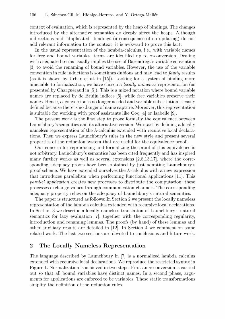
106 L. Sanchez-Gil, M. Hidalgo-Herrero, and Y. Ortega-Mallen
context of evaluation, which is represented by the heap of bindings. The changesintroduced by the alternative semantics do deeply affect the heaps. Althoughindirections and “duplicated” bindings (a consequence of no updating) do notadd relevant information to the context, it is awkward to prove this fact.
In the usual representation of the lambda-calculus, i.e., with variable namesfor free and bound variables, terms are identifed up to α-conversion. Dealingwith α-equated terms usually implies the use of Barendregt’s variable convention[3] to avoid the renaming of bound variables. However, the use of the variableconvention in rule inductions is sometimes dubious and may lead to faulty results(as it is shown by Urban et al. in [15]). Looking for a system of binding moreamenable to formalization, we have chosen a locally nameless representation (aspresented by Chargueraud in [5]). This is a mixed notation where bound variablenames are replaced by de Bruijn indices [6], while free variables preserve theirnames. Hence, α-conversion is no longer needed and variable substitution is easilydefined because there is no danger of name capture. Moreover, this representationis suitable for working with proof assistants like Coq [4] or Isabelle [9].
The present work is the first step to prove formally the equivalence betweenLaunchbury’s semantics and its alternative version. We start by defining a locallynameless representation of the λ-calculus extended with recursive local declara-tions. Then we express Launchbury’s rules in the new style and present severalproperties of the reduction system that are useful for the equivalence proof.
Our concern for reproducing and formalizing the proof of this equivalence isnot arbitrary. Launchbury’s semantics has been cited frequently and has inspiredmany further works as well as several extensions [2,8,13,17], where the corre-sponding adequacy proofs have been obtained by just adapting Launchbury’sproof scheme. We have extended ourselves the λ-calculus with a new expressionthat introduces parallelism when performing functional applications [11]. Thisparallel application creates new processes to distribute the computation; theseprocesses exchange values through communication channels. The correspondingadequacy property relies on the adequacy of Launchbury’s natural semantics.
The paper is structured as follows: In Section 2 we present the locally namelessrepresentation of the lambda calculus extended with recursive local declarations.In Section 3 we describe a locally nameless translation of Launchbury’s naturalsemantics for lazy evaluation [7], together with the corresponding regularity,introduction and renaming lemmas. The proofs (by hand) of these lemmas andother auxiliary results are detailed in [12]. In Section 4 we comment on somerelated work. The last two sections are devoted to conclusions and future work.
2 The Locally Nameless Representation
The language described by Launchbury in [7] is a normalized lambda calculusextended with recursive local declarations. We reproduce the restricted syntax inFigure 1. Normalization is achieved in two steps. First an α-conversion is carriedout so that all bound variables have distinct names. In a second phase, argu-ments for applications are enforced to be variables. These static transformationssimplify the definition of the reduction rules.
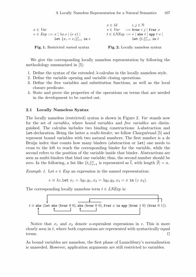
A Locally Nameless Representation for a Natural Semantics 107
x ∈ Vare ∈ Exp ::= x | λx.e | (e x) |
let {xi = ei}ni=1 in e
Fig. 1. Restricted named syntax
x ∈ Id i, j ∈ Nv ∈ Var ::= bvar i j | fvar xt ∈ LNExp ::= v | abs t | app t v |
let {ti}ni=1 in t
Fig. 2. Locally nameless syntax
We give the corresponding locally nameless representation by following themethodology summarized in [5]:
1. Define the syntax of the extended λ-calculus in the locally nameless style.2. Define the variable opening and variable closing operations.3. Define the free variables and substitution functions, as well as the local
closure predicate.4. State and prove the properties of the operations on terms that are needed
in the development to be carried out.
2.1 Locally Nameless Syntax
The locally nameless (restricted) syntax is shown in Figure 2. Var stands nowfor the set of variables, where bound variables and free variables are distin-guished. The calculus includes two binding constructions: λ-abstraction andlet-declaration. Being the latter a multi-binder, we follow Chargueraud [5] andrepresent bound variables with two natural numbers: The first number is a deBruijn index that counts how many binders (abstraction or let) one needs tocross to the left to reach the corresponding binder for the variable, while thesecond refers to the position of the variable inside that binder. Abstractions areseen as multi-binders that bind one variable; thus, the second number should bezero. In the following, a list like {ti}ni=1 is represented as t, with length |t| = n.
Example 1. Let e ∈ Exp an expression in the named representation:
e ≡ λz.let x1 = λy1.y1, x2 = λy2.y2, x3 = x in (z x2).
The corresponding locally nameless term t ∈ LNExp is:
t ≡ abs (let abs (bvar 0 0), abs (bvar 0 0), fvar x in app (bvar 1 0) (bvar 0 1)).
Notice that x1 and x2 denote α-equivalent expressions in e. This is moreclearly seen in t, where both expressions are represented with syntactically equalterms. ��
As bound variables are nameless, the first phase of Launchbury’s normalizationis unneeded. However, application arguments are still restricted to variables.
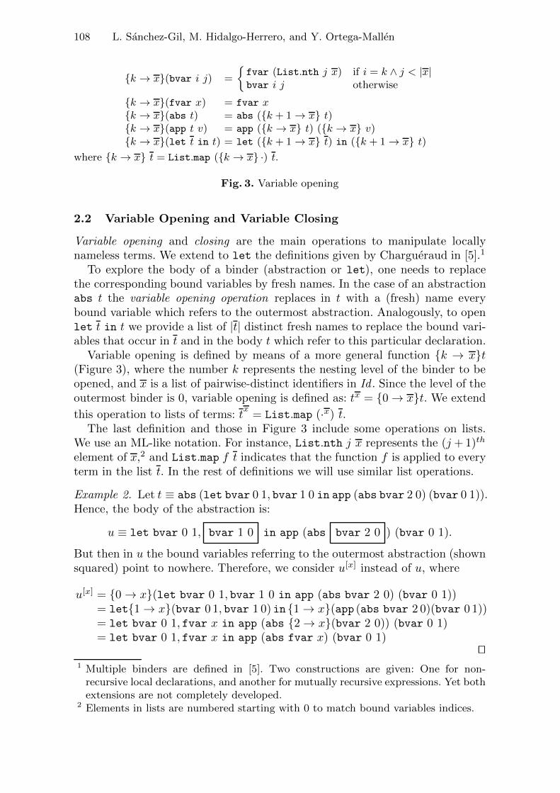
108 L. Sanchez-Gil, M. Hidalgo-Herrero, and Y. Ortega-Mallen
{k → x}(bvar i j) =
{fvar (List.nth j x) if i = k ∧ j < |x|bvar i j otherwise
{k → x}(fvar x) = fvar x{k → x}(abs t) = abs ({k + 1→ x} t){k → x}(app t v) = app ({k → x} t) ({k→ x} v){k → x}(let t in t) = let ({k + 1→ x} t) in ({k + 1→ x} t)
where {k → x} t = List.map ({k → x} ·) t.
Fig. 3. Variable opening
2.2 Variable Opening and Variable Closing
Variable opening and closing are the main operations to manipulate locallynameless terms. We extend to let the definitions given by Chargueraud in [5].1
To explore the body of a binder (abstraction or let), one needs to replacethe corresponding bound variables by fresh names. In the case of an abstractionabs t the variable opening operation replaces in t with a (fresh) name everybound variable which refers to the outermost abstraction. Analogously, to openlet t in t we provide a list of |t| distinct fresh names to replace the bound vari-ables that occur in t and in the body t which refer to this particular declaration.
Variable opening is defined by means of a more general function {k → x}t(Figure 3), where the number k represents the nesting level of the binder to beopened, and x is a list of pairwise-distinct identifiers in Id . Since the level of theoutermost binder is 0, variable opening is defined as: tx = {0→ x}t. We extend
this operation to lists of terms: tx
= List.map (·x) t.The last definition and those in Figure 3 include some operations on lists.
We use an ML-like notation. For instance, List.nth j x represents the (j + 1)th
element of x,2 and List.map f t indicates that the function f is applied to everyterm in the list t. In the rest of definitions we will use similar list operations.
Example 2. Let t ≡ abs (let bvar 0 1, bvar 1 0 in app (abs bvar 2 0) (bvar 0 1)).Hence, the body of the abstraction is:
u ≡ let bvar 0 1, bvar 1 0 in app (abs bvar 2 0 ) (bvar 0 1).
But then in u the bound variables referring to the outermost abstraction (shownsquared) point to nowhere. Therefore, we consider u[x] instead of u, where
u[x] = {0→ x}(let bvar 0 1, bvar 1 0 in app (abs bvar 2 0) (bvar 0 1))= let{1→ x}(bvar 0 1, bvar 1 0) in{1→ x}(app (abs bvar 2 0)(bvar 0 1))= let bvar 0 1, fvar x in app (abs {2→ x}(bvar 2 0)) (bvar 0 1)= let bvar 0 1, fvar x in app (abs fvar x) (bvar 0 1)
��1 Multiple binders are defined in [5]. Two constructions are given: One for non-recursive local declarations, and another for mutually recursive expressions. Yet bothextensions are not completely developed.
2 Elements in lists are numbered starting with 0 to match bound variables indices.
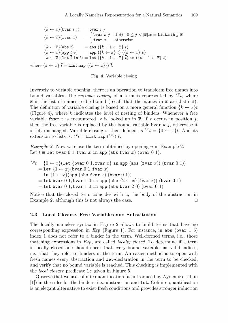
A Locally Nameless Representation for a Natural Semantics 109
{k ← x}(bvar i j) = bvar i j
{k ← x}(fvar x) =
{bvar k j if ∃j : 0 ≤ j < |x|.x = List.nth j xfvar x otherwise
{k ← x}(abs t) = abs ({k + 1← x} t){k ← x}(app t v) = app ({k ← x} t) ({k ← x} v){k ← x}(let t in t) = let ({k + 1← x} t) in ({k + 1← x} t)
where {k ← x} t = List.map ({k ← x} ·) t.
Fig. 4. Variable closing
Inversely to variable opening, there is an operation to transform free names intobound variables. The variable closing of a term is represented by \xt, wherex is the list of names to be bound (recall that the names in x are distinct).The definition of variable closing is based on a more general function {k ← x}t(Figure 4), where k indicates the level of nesting of binders. Whenever a freevariable fvar x is encountered, x is looked up in x. If x occurs in position j,then the free variable is replaced by the bound variable bvar k j, otherwise itis left unchanged. Variable closing is then defined as \xt = {0 ← x}t. And itsextension to lists is: \xt = List.map (\x·) t.
Example 3. Now we close the term obtained by opening u in Example 2.Let t ≡ let bvar 0 1, fvar x in app (abs fvar x) (bvar 0 1).
\xt = {0← x}(let {bvar 0 1, fvar x} in app (abs (fvar x)) (bvar 0 1))= let {1← x}(bvar 0 1, fvar x)in {1← x}(app (abs fvar x) (bvar 0 1))
= let bvar 0 1, bvar 1 0 in app (abs {2← x}(fvar x)) (bvar 0 1)= let bvar 0 1, bvar 1 0 in app (abs bvar 2 0) (bvar 0 1)
Notice that the closed term coincides with u, the body of the abstraction inExample 2, although this is not always the case. ��
2.3 Local Closure, Free Variables and Substitution
The locally nameless syntax in Figure 2 allows to build terms that have nocorresponding expression in Exp (Figure 1). For instance, in abs (bvar 1 5)index 1 does not refer to a binder in the term. Well-formed terms, i.e., thosematching expressions in Exp, are called locally closed. To determine if a termis locally closed one should check that every bound variable has valid indices,i.e., that they refer to binders in the term. An easier method is to open withfresh names every abstraction and let-declaration in the term to be checked,and verify that no bound variable is reached. This checking is implemented withthe local closure predicate lc given in Figure 5.
Observe that we use cofinite quantification (as introduced by Aydemir et al. in[1]) in the rules for the binders, i.e., abstraction and let. Cofinite quantificationis an elegant alternative to exist-fresh conditions and provides stronger induction
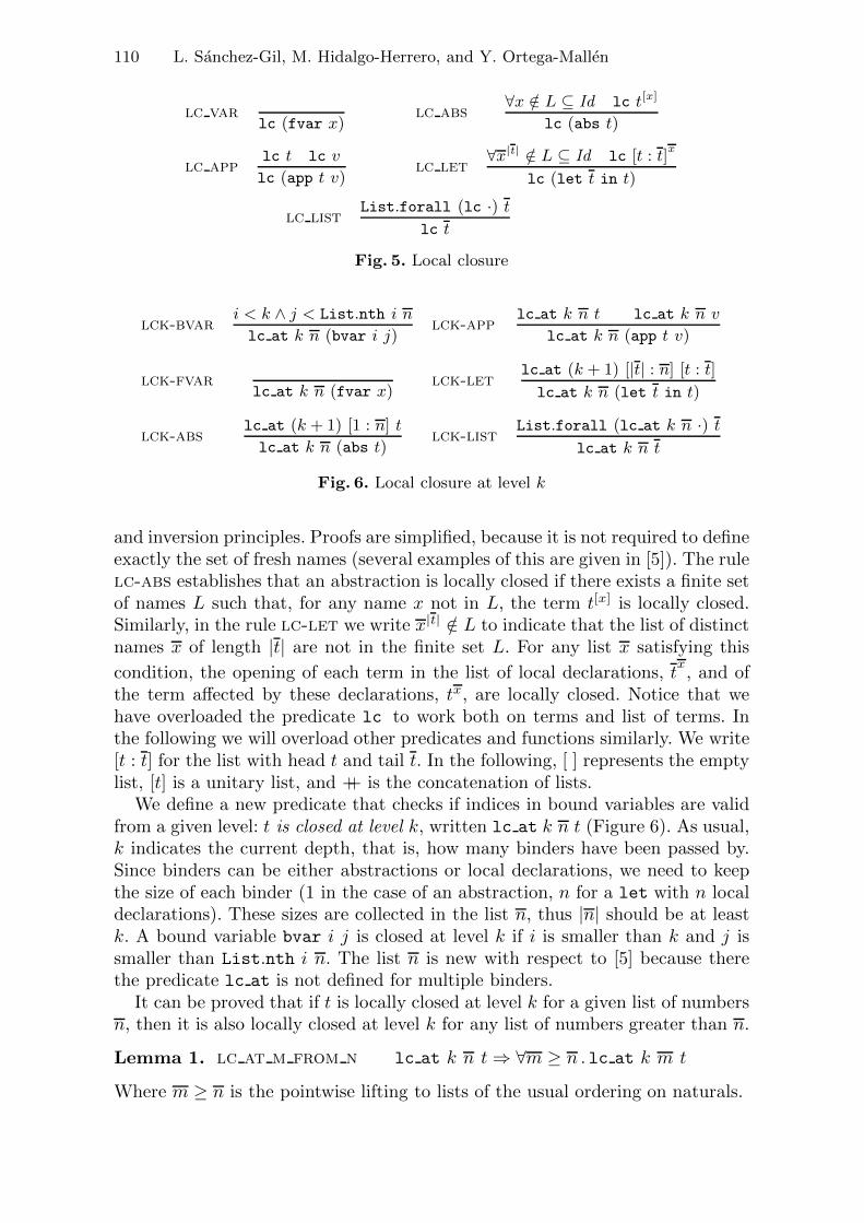
110 L. Sanchez-Gil, M. Hidalgo-Herrero, and Y. Ortega-Mallen
lc varlc (fvar x)
lc abs∀x /∈ L ⊆ Id lc t[x]
lc (abs t)
lc applc t lc v
lc (app t v)lc let
∀x|t| /∈ L ⊆ Id lc [t : t]x
lc (let t in t)
lc listList.forall (lc ·) t
lc t
Fig. 5. Local closure
lck-bvari < k ∧ j < List.nth i n
lc at k n (bvar i j)lck-app
lc at k n t lc at k n v
lc at k n (app t v)
lck-fvarlc at k n (fvar x)
lck-letlc at (k + 1) [|t| : n] [t : t]lc at k n (let t in t)
lck-abslc at (k + 1) [1 : n] t
lc at k n (abs t)lck-list
List.forall (lc at k n ·) tlc at k n t
Fig. 6. Local closure at level k
and inversion principles. Proofs are simplified, because it is not required to defineexactly the set of fresh names (several examples of this are given in [5]). The rulelc-abs establishes that an abstraction is locally closed if there exists a finite setof names L such that, for any name x not in L, the term t[x] is locally closed.Similarly, in the rule lc-let we write x|t| /∈ L to indicate that the list of distinctnames x of length |t| are not in the finite set L. For any list x satisfying this
condition, the opening of each term in the list of local declarations, tx, and of
the term affected by these declarations, tx, are locally closed. Notice that wehave overloaded the predicate lc to work both on terms and list of terms. Inthe following we will overload other predicates and functions similarly. We write[t : t] for the list with head t and tail t. In the following, [ ] represents the emptylist, [t] is a unitary list, and ++ is the concatenation of lists.
We define a new predicate that checks if indices in bound variables are validfrom a given level: t is closed at level k, written lc at k n t (Figure 6). As usual,k indicates the current depth, that is, how many binders have been passed by.Since binders can be either abstractions or local declarations, we need to keepthe size of each binder (1 in the case of an abstraction, n for a let with n localdeclarations). These sizes are collected in the list n, thus |n| should be at leastk. A bound variable bvar i j is closed at level k if i is smaller than k and j issmaller than List.nth i n. The list n is new with respect to [5] because therethe predicate lc at is not defined for multiple binders.
It can be proved that if t is locally closed at level k for a given list of numbersn, then it is also locally closed at level k for any list of numbers greater than n.
Lemma 1. lc at m from n lc at k n t⇒ ∀m ≥ n . lc at k m t
Where m ≥ n is the pointwise lifting to lists of the usual ordering on naturals.
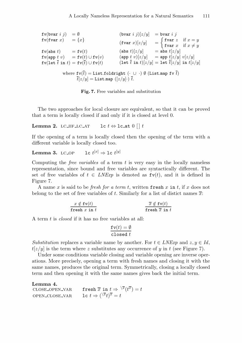
A Locally Nameless Representation for a Natural Semantics 111
fv(bvar i j) = ∅fv(fvar x) = {x}
fv(abs t) = fv(t)fv(app t v) = fv(t) ∪ fv(v)fv(let t in t) = fv(t) ∪ fv(t)
(bvar i j)[z/y] = bvar i j
(fvar x)[z/y] =
{fvar z if x = yfvar x if x = y
(abs t)[z/y] = abs t[z/y](app t v)[z/y] = app t[z/y] v[z/y](let t in t)[z/y] = let t[z/y] in t[z/y]
where fv(t) = List.foldright (· ∪ ·) ∅ (List.map fv t)t[z/y] = List.map ([z/y]·) t.
Fig. 7. Free variables and substitution
The two approaches for local closure are equivalent, so that it can be provedthat a term is locally closed if and only if it is closed at level 0.
Lemma 2. lc iif lc at lc t⇔ lc at 0 [ ] t
If the opening of a term is locally closed then the opening of the term with adifferent variable is locally closed too.
Lemma 3. lc op lc t[x] ⇒ lc t[y]
Computing the free variables of a term t is very easy in the locally namelessrepresentation, since bound and free variables are syntactically different. Theset of free variables of t ∈ LNExp is denoted as fv(t), and it is defined inFigure 7.
A name x is said to be fresh for a term t, written fresh x in t, if x does notbelong to the set of free variables of t. Similarly for a list of distict names x:
x /∈ fv(t)
fresh x in t
x /∈ fv(t)
fresh x in t
A term t is closed if it has no free variables at all:
fv(t) = ∅closed t
Substitution replaces a variable name by another. For t ∈ LNExp and z, y ∈ Id ,t[z/y] is the term where z substitutes any occurrence of y in t (see Figure 7).
Under some conditions variable closing and variable opening are inverse oper-ations. More precisely, opening a term with fresh names and closing it with thesame names, produces the original term. Symmetrically, closing a locally closedterm and then opening it with the same names gives back the initial term.
Lemma 4.close open var fresh x in t⇒ \x(tx) = topen close var lc t⇒ (\xt)x = t
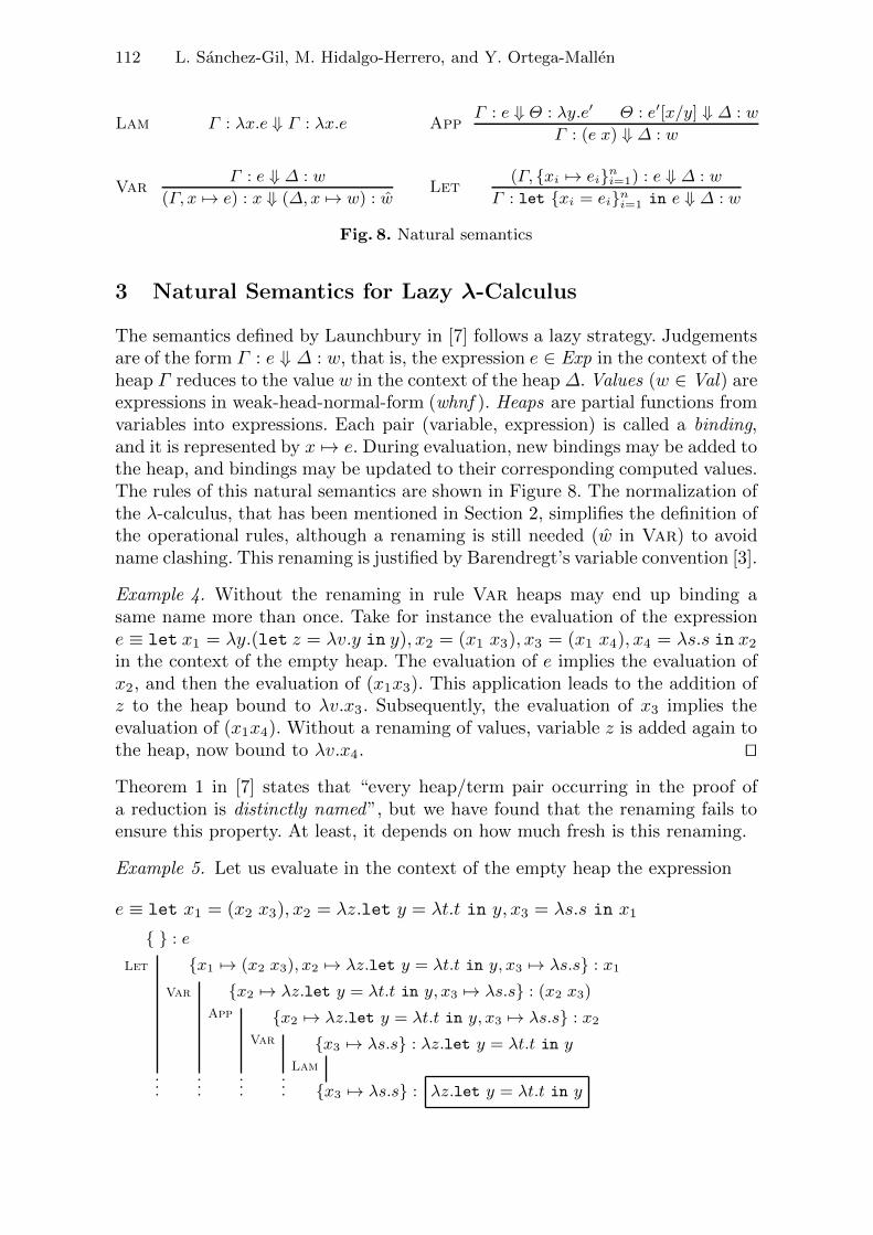
112 L. Sanchez-Gil, M. Hidalgo-Herrero, and Y. Ortega-Mallen
Lam Γ : λx.e ⇓ Γ : λx.e AppΓ : e ⇓ Θ : λy.e′ Θ : e′[x/y] ⇓ Δ : w
Γ : (e x) ⇓ Δ : w
VarΓ : e ⇓ Δ : w
(Γ, x �→ e) : x ⇓ (Δ,x �→ w) : wLet
(Γ, {xi �→ ei}ni=1) : e ⇓ Δ : w
Γ : let {xi = ei}ni=1 in e ⇓ Δ : w
Fig. 8. Natural semantics
3 Natural Semantics for Lazy λ-Calculus
The semantics defined by Launchbury in [7] follows a lazy strategy. Judgementsare of the form Γ : e ⇓ Δ : w, that is, the expression e ∈ Exp in the context of theheap Γ reduces to the value w in the context of the heap Δ. Values (w ∈ Val) areexpressions in weak-head-normal-form (whnf ). Heaps are partial functions fromvariables into expressions. Each pair (variable, expression) is called a binding,and it is represented by x �→ e. During evaluation, new bindings may be added tothe heap, and bindings may be updated to their corresponding computed values.The rules of this natural semantics are shown in Figure 8. The normalization ofthe λ-calculus, that has been mentioned in Section 2, simplifies the definition ofthe operational rules, although a renaming is still needed (w in Var) to avoidname clashing. This renaming is justified by Barendregt’s variable convention [3].
Example 4. Without the renaming in rule Var heaps may end up binding asame name more than once. Take for instance the evaluation of the expressione ≡ let x1 = λy.(let z = λv.y in y), x2 = (x1 x3), x3 = (x1 x4), x4 = λs.s in x2
in the context of the empty heap. The evaluation of e implies the evaluation ofx2, and then the evaluation of (x1x3). This application leads to the addition ofz to the heap bound to λv.x3. Subsequently, the evaluation of x3 implies theevaluation of (x1x4). Without a renaming of values, variable z is added again tothe heap, now bound to λv.x4. ��
Theorem 1 in [7] states that “every heap/term pair occurring in the proof ofa reduction is distinctly named”, but we have found that the renaming fails toensure this property. At least, it depends on how much fresh is this renaming.
Example 5. Let us evaluate in the context of the empty heap the expression
e ≡ let x1 = (x2 x3), x2 = λz.let y = λt.t in y, x3 = λs.s in x1
{ } : e
...
Let {x1 �→ (x2 x3), x2 �→ λz.let y = λt.t in y, x3 �→ λs.s} : x1
...
Var {x2 �→ λz.let y = λt.t in y, x3 �→ λs.s} : (x2 x3)
...
App {x2 �→ λz.let y = λt.t in y, x3 �→ λs.s} : x2
...
Var {x3 �→ λs.s} : λz.let y = λt.t in y
{x3 �→ λs.s} : λz.let y = λt.t in y
Lam
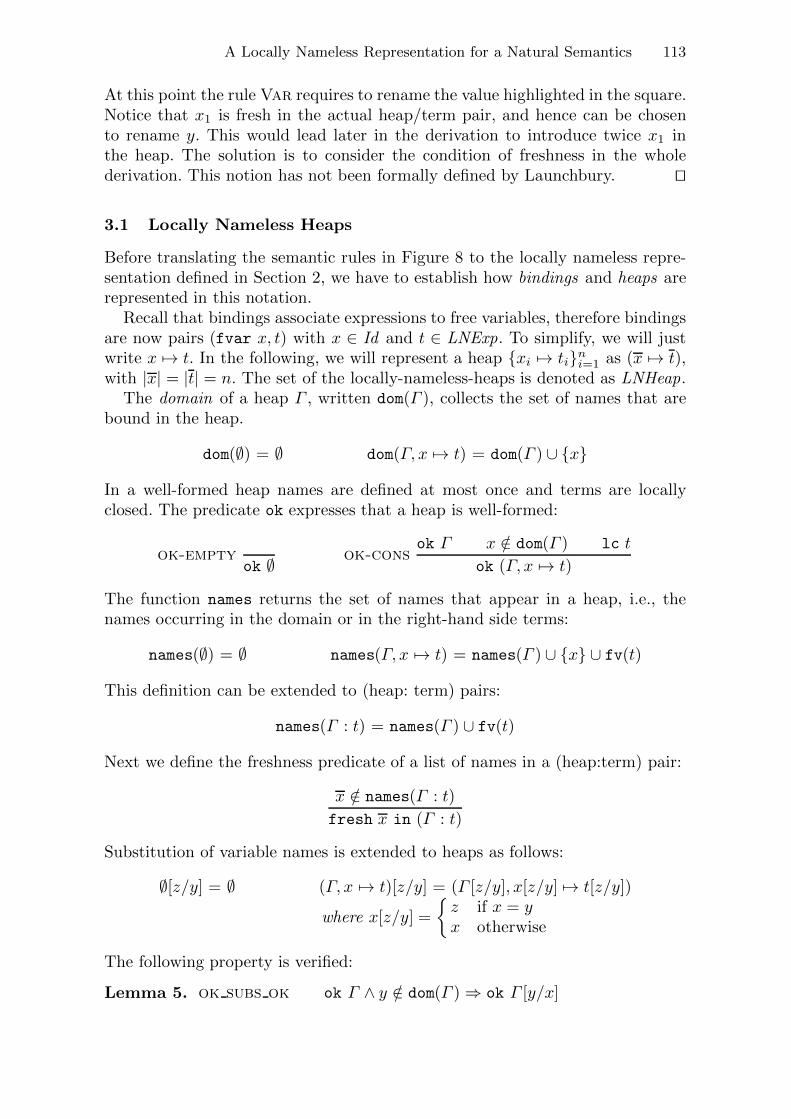
A Locally Nameless Representation for a Natural Semantics 113
At this point the rule Var requires to rename the value highlighted in the square.Notice that x1 is fresh in the actual heap/term pair, and hence can be chosento rename y. This would lead later in the derivation to introduce twice x1 inthe heap. The solution is to consider the condition of freshness in the wholederivation. This notion has not been formally defined by Launchbury. ��
3.1 Locally Nameless Heaps
Before translating the semantic rules in Figure 8 to the locally nameless repre-sentation defined in Section 2, we have to establish how bindings and heaps arerepresented in this notation.
Recall that bindings associate expressions to free variables, therefore bindingsare now pairs (fvar x, t) with x ∈ Id and t ∈ LNExp. To simplify, we will justwrite x �→ t. In the following, we will represent a heap {xi �→ ti}ni=1 as (x �→ t),with |x| = |t| = n. The set of the locally-nameless-heaps is denoted as LNHeap.
The domain of a heap Γ , written dom(Γ ), collects the set of names that arebound in the heap.
dom(∅) = ∅ dom(Γ, x �→ t) = dom(Γ ) ∪ {x}
In a well-formed heap names are defined at most once and terms are locallyclosed. The predicate ok expresses that a heap is well-formed:
ok-emptyok ∅ ok-cons
ok Γ x /∈ dom(Γ ) lc t
ok (Γ, x �→ t)
The function names returns the set of names that appear in a heap, i.e., thenames occurring in the domain or in the right-hand side terms:
names(∅) = ∅ names(Γ, x �→ t) = names(Γ ) ∪ {x} ∪ fv(t)
This definition can be extended to (heap: term) pairs:
names(Γ : t) = names(Γ ) ∪ fv(t)
Next we define the freshness predicate of a list of names in a (heap:term) pair:
x /∈ names(Γ : t)
fresh x in (Γ : t)
Substitution of variable names is extended to heaps as follows:
∅[z/y] = ∅ (Γ, x �→ t)[z/y] = (Γ [z/y], x[z/y] �→ t[z/y])
where x[z/y] =
{z if x = yx otherwise
The following property is verified:
Lemma 5. ok subs ok ok Γ ∧ y /∈ dom(Γ )⇒ ok Γ [y/x]
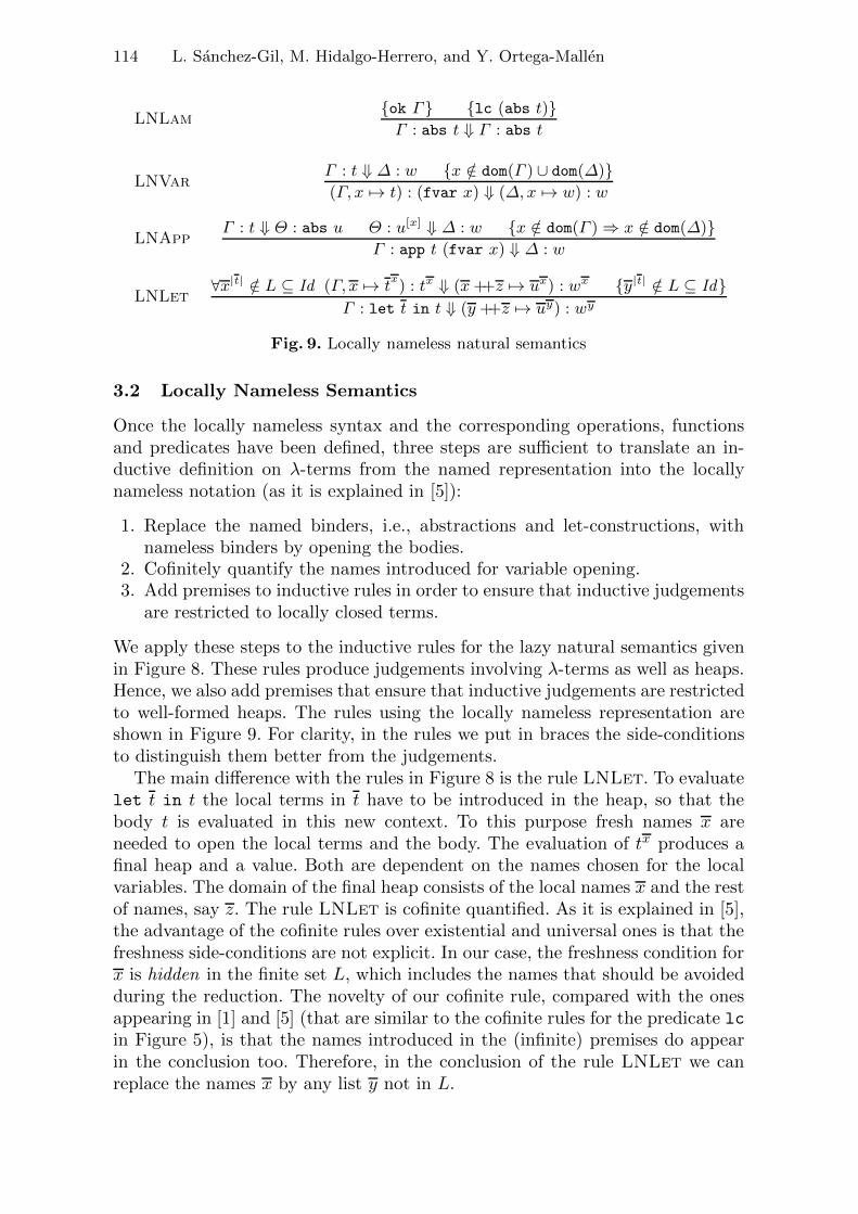
114 L. Sanchez-Gil, M. Hidalgo-Herrero, and Y. Ortega-Mallen
LNLam{ok Γ} {lc (abs t)}Γ : abs t ⇓ Γ : abs t
LNVarΓ : t ⇓ Δ : w {x /∈ dom(Γ ) ∪ dom(Δ)}(Γ, x �→ t) : (fvar x) ⇓ (Δ,x �→ w) : w
LNAppΓ : t ⇓ Θ : abs u Θ : u[x] ⇓ Δ : w {x /∈ dom(Γ )⇒ x /∈ dom(Δ)}
Γ : app t (fvar x) ⇓ Δ : w
LNLet∀x|t| /∈ L ⊆ Id (Γ, x �→ t
x) : tx ⇓ (x++z �→ ux) : wx {y|t| /∈ L ⊆ Id}
Γ : let t in t ⇓ (y ++z �→ uy) : wy
Fig. 9. Locally nameless natural semantics
3.2 Locally Nameless Semantics
Once the locally nameless syntax and the corresponding operations, functionsand predicates have been defined, three steps are sufficient to translate an in-ductive definition on λ-terms from the named representation into the locallynameless notation (as it is explained in [5]):
1. Replace the named binders, i.e., abstractions and let-constructions, withnameless binders by opening the bodies.
2. Cofinitely quantify the names introduced for variable opening.3. Add premises to inductive rules in order to ensure that inductive judgements
are restricted to locally closed terms.
We apply these steps to the inductive rules for the lazy natural semantics givenin Figure 8. These rules produce judgements involving λ-terms as well as heaps.Hence, we also add premises that ensure that inductive judgements are restrictedto well-formed heaps. The rules using the locally nameless representation areshown in Figure 9. For clarity, in the rules we put in braces the side-conditionsto distinguish them better from the judgements.
The main difference with the rules in Figure 8 is the rule LNLet. To evaluatelet t in t the local terms in t have to be introduced in the heap, so that thebody t is evaluated in this new context. To this purpose fresh names x areneeded to open the local terms and the body. The evaluation of tx produces afinal heap and a value. Both are dependent on the names chosen for the localvariables. The domain of the final heap consists of the local names x and the restof names, say z. The rule LNLet is cofinite quantified. As it is explained in [5],the advantage of the cofinite rules over existential and universal ones is that thefreshness side-conditions are not explicit. In our case, the freshness condition forx is hidden in the finite set L, which includes the names that should be avoidedduring the reduction. The novelty of our cofinite rule, compared with the onesappearing in [1] and [5] (that are similar to the cofinite rules for the predicate lcin Figure 5), is that the names introduced in the (infinite) premises do appearin the conclusion too. Therefore, in the conclusion of the rule LNLet we canreplace the names x by any list y not in L.

A Locally Nameless Representation for a Natural Semantics 115
The problem with explicit freshness conditions is that they are associated justto rule instances, while they should apply to the whole reduction proof. Takefor instance the rule LNVar. In the premise the binding x �→ t does no longerbelong to the heap. Hence, a valid reduction for this premise may chose x as fresh(this corresponds to the problem shown in Example 5). We avoid this situationby requiring that x remains undefined in the final heap too. By contrast to therule Var in Figure 8, no renaming of the final value w is needed.
The side-condition of rule LNApp deserves an explanation too. Let us supposethat x is undefined in the initial heap Γ . We must avoid that x is chosen as afresh name during the evaluation of t. For this reason we require that x is definedin the final heap Δ only if x was already defined in Γ . Notice how the body ofthe abstraction, that is u, is open with the name x. This is equivalent to thesubstitution of x for y in the body of the abstraction λy.e′ (see rule App inFigure 8).
A regularity lemma ensures that the judgements produced by this reductionsystem involve only well-formed heaps and locally closed terms.
Lemma 6.regularity Γ : t ⇓ Δ : w ⇒ ok Γ ∧ lc t ∧ ok Δ ∧ lc w
Similarly, Theorem 1 in [7] ensures that the property of being distinctly namedis preserved by the rules in Figure 8. However, as shown in Example 5, thecorrectness of this result requires that freshness is relative to whole reductionproofs instead to the scope of rules.
The next lemma states that names defined in a context heap remain definedafter the evaluation of any term in that context.
Lemma 7.def not lost Γ : t ⇓ Δ : w ⇒ dom(Γ ) ⊆ dom(Δ)
Furthermore, fresh names are introduced only by the rule LNLet and, by theprevious lemma, they remain bound in the final (heap: value) pair. Hence, anyfree variable appearing in a final (heap: value) pair is undefined only if thevariable already occurs in the initial (heap: term) pair.
Lemma 8.add vars Γ : t ⇓ Δ : w
⇒ (x ∈ names(Δ : w)⇒ (x ∈ dom(Δ) ∨ x ∈ names(Γ : t)))
A renaming lemma ensures that the evaluation of a term is independent of thefresh names chosen in the reduction process. Moreover, any name in the contextcan be replaced by a fresh one without changing the meaning of the termsevaluated in that context. In fact, reduction proofs for (heap: term) pairs areunique up to renaming of the variables defined in the context heap.
Lemma 9.renaming Γ : t ⇓ Δ : w ∧ fresh y in (Γ : t) ∧ fresh y in (Δ : w)
⇒ Γ [y/x] : t[y/x] ⇓ Δ[y/x] : w[y/x]
116 L. Sanchez-Gil, M. Hidalgo-Herrero, and Y. Ortega-Mallen
In addition, the renaming lemma permits to prove an introduction lemma for thecofinite rule LNLet which establishes that the corresponding existential rule isadmissible too.
Lemma 10.let intro (Γ, x �→ t
x) : tx ⇓ (x ++z �→ ux) : wx ∧ fresh x in (Γ : let t in t)
⇒ Γ : let t in t ⇓ (x ++z �→ ux) : wx
This result, together with the renaming lemma, justifies that our rule LNLet isequivalent to Launchbury’s rule Let used with normalized terms.
4 Related Work
In order to avoid α-conversion, we first considered a nameless representation likethe de Bruijn notation [6], where variable names are removed and replaced bynatural numbers. But this notation has several drawbacks. First of all, the deBruijn representation is hard to read for humans. Even if we intend to check ourresults with some proof assistant like Coq [4], human readability helps intuition.At a more technical level, the de Bruijn notation does not have a good wayto handle free variables, which are represented by indices, alike to bound vari-ables. This is a serious weakness for our application. Recall that Launchbury’ssemantics uses contexts heaps that collect the bindings for the free variablesthat may occur in the term under evaluation. Any change in the domain of aheap, i.e., adding or deleting a binding, would lead to a shifting of the indices,thus complicating the statement and proof of results. Therefore, we prefer themore manageable locally nameless representation, where bound variable namesare replaced by indices but free variables keep their names. This mixed notationcombines the advantages of both named and nameless representations. On theone hand, α-conversion is avoided all the same. On the other hand, terms stayreadable and easy to manipulate.
There exists in the literature different proposals for a locally nameless rep-resentation, and many works using these representations. Chargueraud offers in[5] a brief survey on these works, that we recommend to the interested reader.
Launchbury (implicitly) assumes Barendregt’s variable convention [3] twice in[7]. First when he defines his operational semantics only for normalized λ-terms(i.e. every binder in a term binds a distinct name, which is also distinct fromany free variable); and second, when he requires a (fresh) renaming of the valuesin the rule Var (see Figure 8). Urban, Berghofer and Norrish propose in [15] amethod to strengthen an induction principle (corresponding to some inductiverelation), so that Barendregt’s variable convention comes already built in theprinciple. Unfortunately, we cannot apply these ideas to Launchbury’s semantics,because the semantic rules (shown in Figure 8) do not satisfy the conditions thatguarantee the variable convention compatibility, as described in [15]. In fact, aswe have already pointed out, Launchbury’s Theorem 1 (in [7]) is only correct ifthe renaming required in each application of the rule Var is fresh in the wholereduction proof. Therefore, we cannot use directly Urban’s nominal package for
A Locally Nameless Representation for a Natural Semantics 117
Isabelle/HOL [14] (including its recent extensions for general bindings describedin [16]).
Nevertheless, Urban et al. achieve the “inclusion” of the variable conventionin an induction principle by adding to each induction rule a side condition whichexpresses that the set of bound variables (i.e., those that appear in a bindingposition in the rule) are fresh in some induction context ([15]). Furthermore,this context is required to be finitely supported. This is closely related to thecofinite quantification that we have used for the rule LNLet in Figure 9. Besides,one important condition to ensure the variable convention compatibility is theequivariance of the functions and predicates occurring in the induction rules.Equivariance is a notion from nominal logic [10]. A relation is equivariant if itis preserved by permutation of names. Although we have not proven that thereduction relation defined by the rules in Figure 9 is equivariant, our renaminglemma (Lemma 9) establishes a similar result, that is, the reduction relation ispreserved by (fresh) renaming.
5 Conclusions
We have used a more modern approach to binding, i.e., a locally nameless repre-sentation for the λ-calculus extended with mutually recursive local declarations.With this representation the reduction rule for local declarations implies theintroduction of fresh names. We have used neither an existential nor a universalrule for this case. Instead, we have opted for a cofinite rule as introduced byAydemir et al. in [1]. Freshness conditions are usually considered in each ruleindividually. Nevertheless, this technique produces name clashing when consider-ing whole reduction proofs. A solution might be to decorate judgements with theset of forbidden names and indicate how to modify this set during the reductionprocess (this approach has been taken by Sestoft in [13]). However, this couldbe too restrictive in many occasions. Besides, existential rules are not easy todeal with because each reduction is obtained just for one specific list of names.If any of the names in this list causes a name clashing with other reductionproofs, then it is cumbersome to demonstrate that an alternative reduction for afresh list does exist. Cofinite quantification has allowed us to solve this problembecause in a single step reductions are guaranteed for an infinite number of listsof names. Nonetheless, our introduction lemma (Lemma 10) guarantees that amore conventional exists-fresh rule is correct in our reduction system too.
The cofinite quantification that we have used in our semantic rules is morecomplex than those in [1] and [5]. Our cofinite rule LNLet in Figure 9 introducesquantified variables in the conclusion as well, as the latter depends on the chosennames.
Compared to Launchbury’s original semantic rules, our locally nameless rulesinclude several extra side-conditions. Some of these conditions require that heapsand terms are well-formed (like in rule LNLam). The rest of side-conditionsexpress restrictions on the choice of fresh names. These restrictions, togetherwith the cofinite quantification, fix the problem with the renaming in rule Varthat we have shown in Example 5.
118 L. Sanchez-Gil, M. Hidalgo-Herrero, and Y. Ortega-Mallen
For our locally nameless semantics we have shown a regularity lemma (Lemma6) which ensures that every term and heap involved in a reduction proof is well-formed, and with a renaming lemma (Lemma 9) which indicates that the choiceof names (free variables) is irrelevant as long as they are fresh enough. A heapmay be seen as a multiple binder. Actually, the names defined (bound) in a heapcan be replaced by other names, provided that terms keep their meaning in thecontext represented by the heap. Our renaming lemma ensures that whenever aheap is renamed with fresh names, reduction proofs are preserved. This renaminglemma is essential in rule induction proofs for some properties of the reductionsystem. More concretely, when one combines several reduction proofs comingfrom two or more premises in a reduction rule (for instance, in rule LNApp inFigure 9).
In summary, the contributions of this paper are:
1. A locally nameless representation of the λ-calculus extended with recursivelocal declarations;
2. A locally nameless version of the inductive rules of Launchbury’s naturalsemantics for lazy evaluation;
3. A new version of cofinite rules where the variables quantified in the premisesdo appear in the conclusion too;
4. A set of interesting properties of our reduction system, including the regu-larity, the introduction and the renaming lemmas; and
5. A way to guarantee Barendregt’s variable convention by redefining Launch-bury’s semantic rules with cofinite quantification and extra side-conditions.
6 Future Work
Our future tasks include the implementation in the proof assistant Coq [4] of thenatural semantics redefined in this paper, and the formalization of the proofs forthe lemmas given (regularity, renaming, introduction, etc.), which at present arejust paper-and-pencil proofs. We will use this implementation to prove formallythe equivalence of Launchbury’s natural semantics with the alternative versiongiven also in [7]. As we mentioned in Section 1, this alternative version differsfrom the original one in the introduction of indirections during β-reduction andthe elimination of updates. At present we are working on the definition (using thelocally nameless representation) of two intermediate semantics, one introducingindirections and the other without updates. Then, we will establish equivalencerelations between the heaps obtained by each semantics, which makes able toprove the equivalence of the original natural semantics and the alternative onethrough the intermediate semantics.
Acknowledgments. This work is partially supported by the projects: TIN2009-14599-C03-01 and S2009/TIC-1465.

A Locally Nameless Representation for a Natural Semantics 119
References
1. Aydemir, B.E., Chargueraud, A., Pierce, B.C., Pollack, R., Weirich, S.: Engineeringformal metatheory. In: ACM Symposium on Principles of Programming Languages,POPL 2008, pp. 3–15. ACM Press (2008)
2. Baker-Finch, C., King, D., Trinder, P.W.: An operational semantics for parallellazy evaluation. In: ACM-SIGPLAN International Conference on Functional Pro-gramming (ICFP 2000), pp. 162–173. ACM Press (2000)
3. Barendregt, H.P.: The Lambda Calculus: Its Syntax and Semantics. Studies inLogic and the Foundations of Mathematics, vol. 103. North-Holland (1984)
4. Bertot, Y.: Coq in a hurry. CoRR, abs/cs/0603118 (2006)5. Chargueraud, A.: The locally nameless representation. Journal of Automated Rea-
soning, 1–46 (2011)6. de Bruijn, N.G.: Lambda calculus notation with nameless dummies, a tool for
automatic formula manipulation, with application to the Church-Rosser theorem.Indagationes Mathematicae 75(5), 381–392 (1972)
7. Launchbury, J.: A natural semantics for lazy evaluation. In: ACM Symposiumon Principles of Programming Languages, POPL 1993, pp. 144–154. ACM Press(1993)
8. Nakata, K., Hasegawa, M.: Small-step and big-step semantics for call-by-need.CoRR, abs/0907.4640 (2009)
9. Nipkow, T., Paulson, L.C., Wenzel, M.T.: Isabelle/HOL — A Proof Assistant forHigher-Order Logic. LNCS, vol. 2283. Springer, Heidelberg (2002)
10. Pitts, A.M.: Nominal logic, a first order theory of names and binding. Informationand Computation 186(2), 165–193 (2003)
11. Sanchez-Gil, L., Hidalgo-Herrero, M., Ortega-Mallen, Y.: An Operational Seman-tics for Distributed Lazy Evaluation. In: Trends in Functional Programming,vol. 10, pp. 65–80. Intellect (2010)
12. Sanchez-Gil, L., Hidalgo-Herrero, M., Ortega-Mallen, Y.: A locally nameless rep-resentation for a natural semantics for lazy evaluation. Technical Report 01/12,Dpt. Sistemas Informaticos y Computacion. Universidad Complutense de Madrid(2012), http://maude.sip.ucm.es/eden-semantics/
13. Sestoft, P.: Deriving a lazy abstract machine. Journal of Functional Program-ming 7(3), 231–264 (1997)
14. Urban, C.: Nominal techniques in Isabelle/HOL. Journal of Automatic Reason-ing 40(4), 327–356 (2008)
15. Urban, C., Berghofer, S., Norrish, M.: Barendregt’s Variable Convention in RuleInductions. In: Pfenning, F. (ed.) CADE 2007. LNCS (LNAI), vol. 4603, pp. 35–50.Springer, Heidelberg (2007)
16. Urban, C., Kaliszyk, C.: General Bindings and Alpha-Equivalence in Nominal Is-abelle. In: Barthe, G. (ed.) ESOP 2011. LNCS, vol. 6602, pp. 480–500. Springer,Heidelberg (2011)
17. van Eekelen, M., de Mol, M.: Reflections on Type Theory, λ-calculus, and the Mind.Essays dedicated to Henk Barendregt on the Occasion of his 60th Birthday, chapterProving Lazy Folklore with Mixed Lazy/Strict Semantics, pp. 87–101. RadboudUniversity Nijmegen (2007)

134 Capıtulo 5. Publicaciones
The Role of Indirections in LazyNatural Semantics
Lidia Sanchez-Gil1, Mercedes Hidalgo-Herrero2, and YolandaOrtega-Mallen3(B)
1 Facultad de Informatica, Universidad Complutense de Madrid, Madrid, Spain2 Facultad de Educacion, Universidad Complutense de Madrid, Madrid, Spain
3 Facultad de CC. Matematicas, Universidad Complutense de Madrid, Madrid, [email protected]
Abstract. Launchbury defines a natural semantics for lazy evaluationand proposes an alternative version which introduces indirections, elimi-nates blackholes and does not update closures. Equivalence of both seman-tics is not straightforward. In this paper we focus on the introduction ofindirections during β-reduction and study how the heaps, i.e., the sets ofbindings, obtained with this kind of evaluation do relate with the heapsproduced by substitution. As a heap represents the context of evaluationfor a term, we first define an equivalence that identifies terms with thesame meaning under a given context. This notion of context equivalenceis extended to heaps. Finally, we define a relation between heap/term pairsto establish the equivalence between Launchbury’s alternative naturalsemantics and its corresponding version without indirections.
1 Motivation
More than twenty years have elapsed since Launchbury first presented in [9]a natural semantics for lazy evaluation (call-by-need), a key contribution tothe semantic foundation for non-strict functional programming languages likeHaskell or Clean. Throughout these years, Launchbury’s semantics has been citedfrequently and has inspired many further works as well as several extensions likein [2,8,10,13,17,20]. The success of Lanchbury’s proposal resides in its simplicity.Expressions are evaluated with respect to a context, which is represented by aheap of bindings, that is, (variable, expression) pairs. This heap is explicitlymanaged to make possible the sharing of bindings, thus, modeling laziness.
In order to prove that this lazy (operational) semantics is correct and compu-tationally adequate with respect to a standard denotational semantics, Launch-bury introduces some variations in the operational semantics. On the one hand,the update of bindings with their computed values is an operational notion with-out counterpart in the standard denotational semantics, so that the alternativenatural semantics does no longer update bindings and becomes a call-by-namesemantics. On the other hand, functional application is modeled denotationallyby extending the environment with a variable bound to a value. This new vari-able represents the formal parameter of the function, while the value corresponds
c© Springer-Verlag Berlin Heidelberg 2015A. Voronkov and I. Virbitskaite (Eds.): PSI 2014, LNCS 8974, pp. 288–303, 2015.DOI: 10.1007/978-3-662-46823-4 24
The Role of Indirections in Lazy Natural Semantics 289
to the actual argument. For a closer approach to this mechanism, in the alter-native semantics applications are carried out by introducing indirections, i.e.,variables bound to variables, instead of by performing the β-reduction throughsubstitution. Besides, the denotation “undefined” indicates that there is no valueassociated to the expression being evaluated, but there is no indication of thereason for that. By contrast, in the operational semantics there are two possi-bilities for not reaching a value: either the reduction gets blocked if no rule isapplicable, or the reduction never stops. The first case occurs in the originalsemantics when reducing self-references (blackhole). The rules in the alternativesemantics guarantee that reductions never reach a blackhole.
Alas, the proof of the equivalence of the natural semantics and its alternativeversion is detailed nowhere, and a simple induction turns out to be insufficient.The context-heap semantics is too sensitive to the changes introduced by thealternative rules. Intuitively, both reduction systems should lead to the sameresults. However, this cannot be directly established since final values may con-tain free variables that are dependent on the context of evaluation, which isrepresented by the heap of bindings. The lack of update leads to the duplicationof bindings, but is awkward to prove that duplicated bindings, as well as indirec-tions, do not add relevant information to the context. Therefore, our challenge isto establish a way of relating the heaps and values obtained with each reductionsystem, and to prove that the semantics are equivalent, so that any reduction ofa term in one of the systems has its counterpart in the other. To facilitate thistask we consider separately the no updating and the introduction of indirections.
In this paper we investigate the effect of introducing indirections in a settingwithout updates, and we analyze the similarities and differences between thereductions proofs obtained with and without indirections. Indirections have alsobeen used in [8] to model communication channels between processes.
Wewant to identify terms up toα-conversion, but dealingwithα-equated termsusually implies the use of Barendregt’s variable convention [3] to avoid the renam-ing of bound variables. However, the use of the variable convention is sometimesdubious and may lead to faulty results (as it is shown by Urban et al. in [18]). More-over, we intend to formalize our results with the help of some proof assistant likeCoq [4] or Isabelle [11]. Looking for a binding system susceptible of formalization,we have chosen a locally nameless representation (as presented by Chargueraudin [6]). This is a mixed notation where bound variable names are replaced by deBruijn indices [7], while free variables preserve their names. This is suitable in ourcase because context heaps collect free variables whose names we are interestedin preserving in order to identify them more easily. A locally nameless version ofLaunchbury’s natural semantics has been presented by the authors in [14,15].
Others are revisiting Launchbury’s semantics too. For instance, Breitner hasformally proven in [5] the correctness of the natural semantics by using Isabelle’snominal package [19], and presently he is working on the formalization of theadequacy. While Breitner is exclusively interested in formalizing the proofs, wehave a broader objective: To analyze the effect of introducing indirections in thecontext heaps, and the correspondence between heap/value pairs obtained with
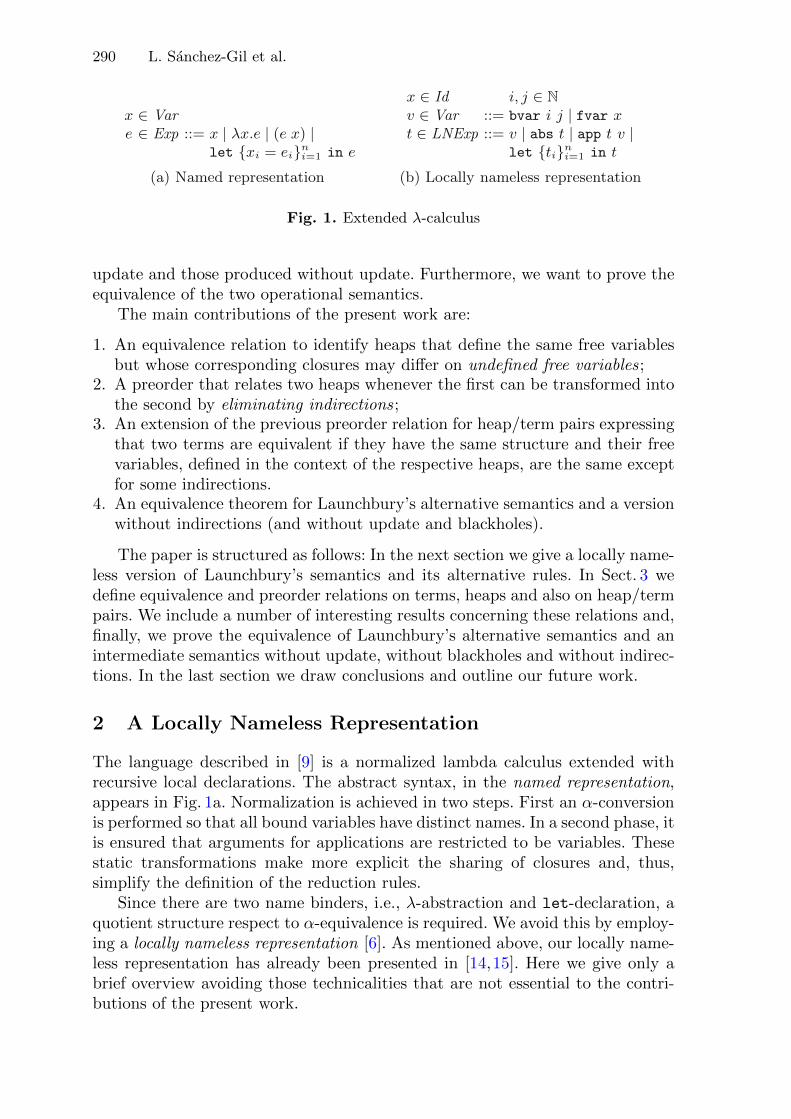
290 L. Sanchez-Gil et al.
x ∈ Vare ∈ Exp ::= x | λx.e | (e x) |
let {xi = ei}ni=1 in e
(a) Named representation
x ∈ Id i, j ∈ N
v ∈ Var ::= bvar i j | fvar xt ∈ LNExp ::= v | abs t | app t v |
let {ti}ni=1 in t
(b) Locally nameless representation
Fig. 1. Extended λ-calculus
update and those produced without update. Furthermore, we want to prove theequivalence of the two operational semantics.
The main contributions of the present work are:
1. An equivalence relation to identify heaps that define the same free variablesbut whose corresponding closures may differ on undefined free variables;
2. A preorder that relates two heaps whenever the first can be transformed intothe second by eliminating indirections;
3. An extension of the previous preorder relation for heap/term pairs expressingthat two terms are equivalent if they have the same structure and their freevariables, defined in the context of the respective heaps, are the same exceptfor some indirections.
4. An equivalence theorem for Launchbury’s alternative semantics and a versionwithout indirections (and without update and blackholes).
The paper is structured as follows: In the next section we give a locally name-less version of Launchbury’s semantics and its alternative rules. In Sect. 3 wedefine equivalence and preorder relations on terms, heaps and also on heap/termpairs. We include a number of interesting results concerning these relations and,finally, we prove the equivalence of Launchbury’s alternative semantics and anintermediate semantics without update, without blackholes and without indirec-tions. In the last section we draw conclusions and outline our future work.
2 A Locally Nameless Representation
The language described in [9] is a normalized lambda calculus extended withrecursive local declarations. The abstract syntax, in the named representation,appears in Fig. 1a. Normalization is achieved in two steps. First an α-conversionis performed so that all bound variables have distinct names. In a second phase, itis ensured that arguments for applications are restricted to be variables. Thesestatic transformations make more explicit the sharing of closures and, thus,simplify the definition of the reduction rules.
Since there are two name binders, i.e., λ-abstraction and let-declaration, aquotient structure respect to α-equivalence is required. We avoid this by employ-ing a locally nameless representation [6]. As mentioned above, our locally name-less representation has already been presented in [14,15]. Here we give only abrief overview avoiding those technicalities that are not essential to the contri-butions of the present work.
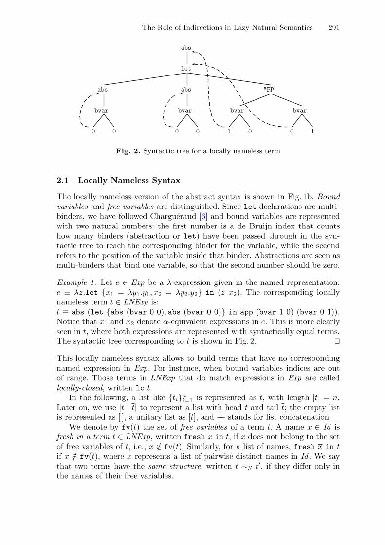
The Role of Indirections in Lazy Natural Semantics 291
abs
let
abs abs app
bvar bvar bvar bvar
0 0 0 0 01 0 1
Fig. 2. Syntactic tree for a locally nameless term
2.1 Locally Nameless Syntax
The locally nameless version of the abstract syntax is shown in Fig. 1b. Boundvariables and free variables are distinguished. Since let-declarations are multi-binders, we have followed Chargueraud [6] and bound variables are representedwith two natural numbers: the first number is a de Bruijn index that countshow many binders (abstraction or let) have been passed through in the syn-tactic tree to reach the corresponding binder for the variable, while the secondrefers to the position of the variable inside that binder. Abstractions are seen asmulti-binders that bind one variable, so that the second number should be zero.
Example 1. Let e ∈ Exp be a λ-expression given in the named representation:e ≡ λz.let {x1 = λy1.y1, x2 = λy2.y2} in (z x2). The corresponding locallynameless term t ∈ LNExp is:t ≡ abs (let {abs (bvar 0 0), abs (bvar 0 0)} in app (bvar 1 0) (bvar 0 1)).Notice that x1 and x2 denote α-equivalent expressions in e. This is more clearlyseen in t, where both expressions are represented with syntactically equal terms.The syntactic tree corresponding to t is shown in Fig. 2. ��This locally nameless syntax allows to build terms that have no correspondingnamed expression in Exp. For instance, when bound variables indices are outof range. Those terms in LNExp that do match expressions in Exp are calledlocally-closed, written lc t.
In the following, a list like {ti}ni=1 is represented as t, with length |t| = n.
Later on, we use [t : t] to represent a list with head t and tail t; the empty listis represented as [ ], a unitary list as [t], and ++ stands for list concatenation.
We denote by fv(t) the set of free variables of a term t. A name x ∈ Id isfresh in a term t ∈ LNExp, written fresh x in t, if x does not belong to the setof free variables of t, i.e., x /∈ fv(t). Similarly, for a list of names, fresh x in tif x /∈ fv(t), where x represents a list of pairwise-distinct names in Id . We saythat two terms have the same structure, written t ∼S t′, if they differ only inthe names of their free variables.
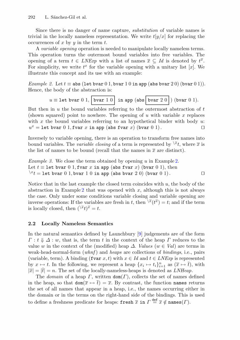
292 L. Sanchez-Gil et al.
Since there is no danger of name capture, substitution of variable names istrivial in the locally nameless representation. We write t[y/x] for replacing theoccurrences of x by y in the term t.
A variable opening operation is needed to manipulate locally nameless terms.This operation turns the outermost bound variables into free variables. Theopening of a term t ∈ LNExp with a list of names x ⊆ Id is denoted by tx.For simplicity, we write tx for the variable opening with a unitary list [x]. Weillustrate this concept and its use with an example:
Example 2. Let t ≡ abs (let bvar 0 1, bvar 1 0 in app (abs bvar 2 0) (bvar 0 1)).Hence, the body of the abstraction is:
u ≡ let bvar 0 1, bvar 1 0 in app (abs bvar 2 0 ) (bvar 0 1).
But then in u the bound variables referring to the outermost abstraction of t(shown squared) point to nowhere. The opening of u with variable x replaceswith x the bound variables referring to an hypothetical binder with body u:ux = let bvar 0 1, fvar x in app (abs fvar x) (bvar 0 1) . ��Inversely to variable opening, there is an operation to transform free names intobound variables. The variable closing of a term is represented by \xt, where x isthe list of names to be bound (recall that the names in x are distinct).
Example 3. We close the term obtained by opening u in Example 2.Let t ≡ let bvar 0 1, fvar x in app (abs fvar x) (bvar 0 1), then\xt = let bvar 0 1, bvar 1 0 in app (abs bvar 2 0) (bvar 0 1) . ��Notice that in the last example the closed term coincides with u, the body of theabstraction in Example 2 that was opened with x, although this is not alwaysthe case. Only under some conditions variable closing and variable opening areinverse operations: If the variables are fresh in t, then \x(tx) = t; and if the termis locally closed, then (\xt)x = t.
2.2 Locally Nameless Semantics
In the natural semantics defined by Launchbury [9] judgements are of the formΓ : t ⇓ Δ : w, that is, the term t in the context of the heap Γ reduces to thevalue w in the context of the (modified) heap Δ. Values (w ∈ Val) are terms inweak-head-normal-form (whnf ) and heaps are collections of bindings, i.e., pairs(variable, term). A binding (fvar x, t) with x ∈ Id and t ∈ LNExp is representedby x → t. In the following, we represent a heap {xi → ti}n
i=1 as (x → t), with|x| = |t| = n. The set of the locally-nameless-heaps is denoted as LNHeap.
The domain of a heap Γ , written dom(Γ ), collects the set of names definedin the heap, so that dom(x → t) = x. By contrast, the function names returnsthe set of all names that appear in a heap, i.e., the names occurring either inthe domain or in the terms on the right-hand side of the bindings. This is used
to define a freshness predicate for heaps: fresh x in Γdef= x /∈ names(Γ ).
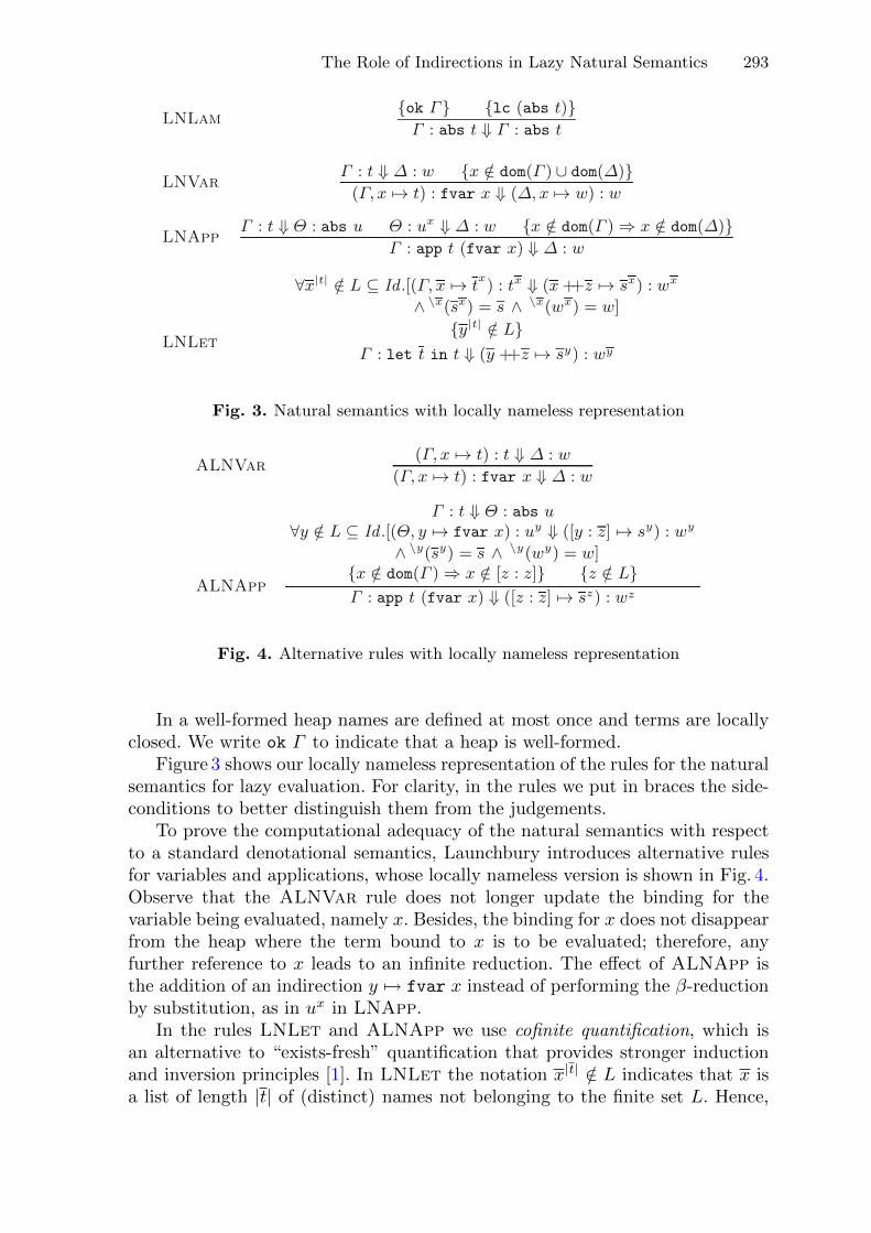
The Role of Indirections in Lazy Natural Semantics 293
LNLam{ok Γ} {lc (abs t)}
Γ : abs t ⇓ Γ : abs t
LNVarΓ : t ⇓ Δ : w {x /∈ dom(Γ ) ∪ dom(Δ)}(Γ, x t) : fvar x ⇓ (Δ, x w) : w
LNAppΓ : t ⇓ Θ : abs u Θ : ux ⇓ Δ : w {x /∈ dom(Γ ) ⇒ x /∈ dom(Δ)}
Γ : app t (fvar x) ⇓ Δ : w
LNLet
∀x|t| /∈ L ⊆ Id .[(Γ, x tx) : tx ⇓ (x ++z sx) : wx
∧ \x(sx) = s ∧ \x(wx) = w]
{y|t| /∈ L}Γ : let t in t ⇓ (y ++z sy) : wy
Fig. 3. Natural semantics with locally nameless representation
ALNVar(Γ, x t) : t ⇓ Δ : w
(Γ, x t) : fvar x ⇓ Δ : w
ALNApp
Γ : t ⇓ Θ : abs u∀y /∈ L ⊆ Id .[(Θ, y fvar x) : uy ⇓ ([y : z] sy) : wy
∧ \y(sy) = s ∧ \y(wy) = w]{x /∈ dom(Γ ) ⇒ x /∈ [z : z]} {z /∈ L}Γ : app t (fvar x) ⇓ ([z : z] sz) : wz
Fig. 4. Alternative rules with locally nameless representation
In a well-formed heap names are defined at most once and terms are locallyclosed. We write ok Γ to indicate that a heap is well-formed.
Figure 3 shows our locally nameless representation of the rules for the naturalsemantics for lazy evaluation. For clarity, in the rules we put in braces the side-conditions to better distinguish them from the judgements.
To prove the computational adequacy of the natural semantics with respectto a standard denotational semantics, Launchbury introduces alternative rulesfor variables and applications, whose locally nameless version is shown in Fig. 4.Observe that the ALNVar rule does not longer update the binding for thevariable being evaluated, namely x. Besides, the binding for x does not disappearfrom the heap where the term bound to x is to be evaluated; therefore, anyfurther reference to x leads to an infinite reduction. The effect of ALNApp isthe addition of an indirection y → fvar x instead of performing the β-reductionby substitution, as in ux in LNApp.
In the rules LNLet and ALNApp we use cofinite quantification, which isan alternative to “exists-fresh” quantification that provides stronger inductionand inversion principles [1]. In LNLet the notation x|t| /∈ L indicates that x isa list of length |t| of (distinct) names not belonging to the finite set L. Hence,

294 L. Sanchez-Gil et al.
although there are not explicit freshness side-conditions in the rules, the finiteset L represents somehow the names that should be avoided during a reductionproof. Among infinite possible combinations for x, the set of names y is chosenfor the reduction. The list z represents the rest of names defined in the heapwhich is obtained after the reduction. Notice how variable opening is used toexpress that the final heap and value may depend on the names that have beenchosen. For instance, in LNLet, wx indicates that it depends on the names x,but there is a common basis w . Moreover, it is required that this basis does notcontain occurrences of x; this is expressed by \x(wx) = w. A detailed explanationof these semantic rules can be found in [14–16].
In the following, the natural semantics (rules in Fig. 3) is referred as NS, andthe alternative semantics (rules LNLam, LNLet and those in Fig. 4) as ANS.We write ⇓A for reductions in ANS. Launchbury proves in [9] the correctness ofNS with respect to a standard denotational semantics, and a similar result forANS is easily obtained (as the authors of this paper have done in [12]). Therefore,NS and ANS are “denotationally” equivalent in the sense that if an expressionis reducible (in some heap context) by both semantics then the obtained valueshave the same denotation. But this is insufficient for our purposes, because wewant to ensure that if for some (heap : term) pair a reduction exists in anyof the semantics, then there must exist a reduction in the other too and thefinal heaps must be related. The changes in ANS might seem to involve noserious difficulties to prove the latter result. Unfortunately things are not soeasy. On the one hand, the alternative rule for variables transforms the originalcall-by-need semantics into a call-by-name semantics because bindings are notupdated and computed values are no longer shared. Moreover, in the originalsemantics the reduction of a self-reference gets blocked (blackhole), while in thealternative semantics self-references yield infinite reductions. On the other hand,the addition of indirections complicates the task of comparing the (heap : value)pairs obtained by each reduction system, as one may need to follow a chainof indirections to get the term bound to a variable. We deal separately witheach modification and introduce two intermediate semantics: (1) the No-updateNatural Semantics (NNS) with the rules of NS (Fig. 3) except for the variablerule, that corresponds to the one in the alternative version, i.e., ALNVar inFig. 4; and (2) the Indirection Natural Semantics (INS) with the rules of NS butfor the application rule, that corresponds to the alternative ALNApp rule inFig. 4. We use ⇓N to represent reductions of NNS and ⇓I for those of INS.
The following table summarizes the characteristics of the four natural seman-tics defined above:
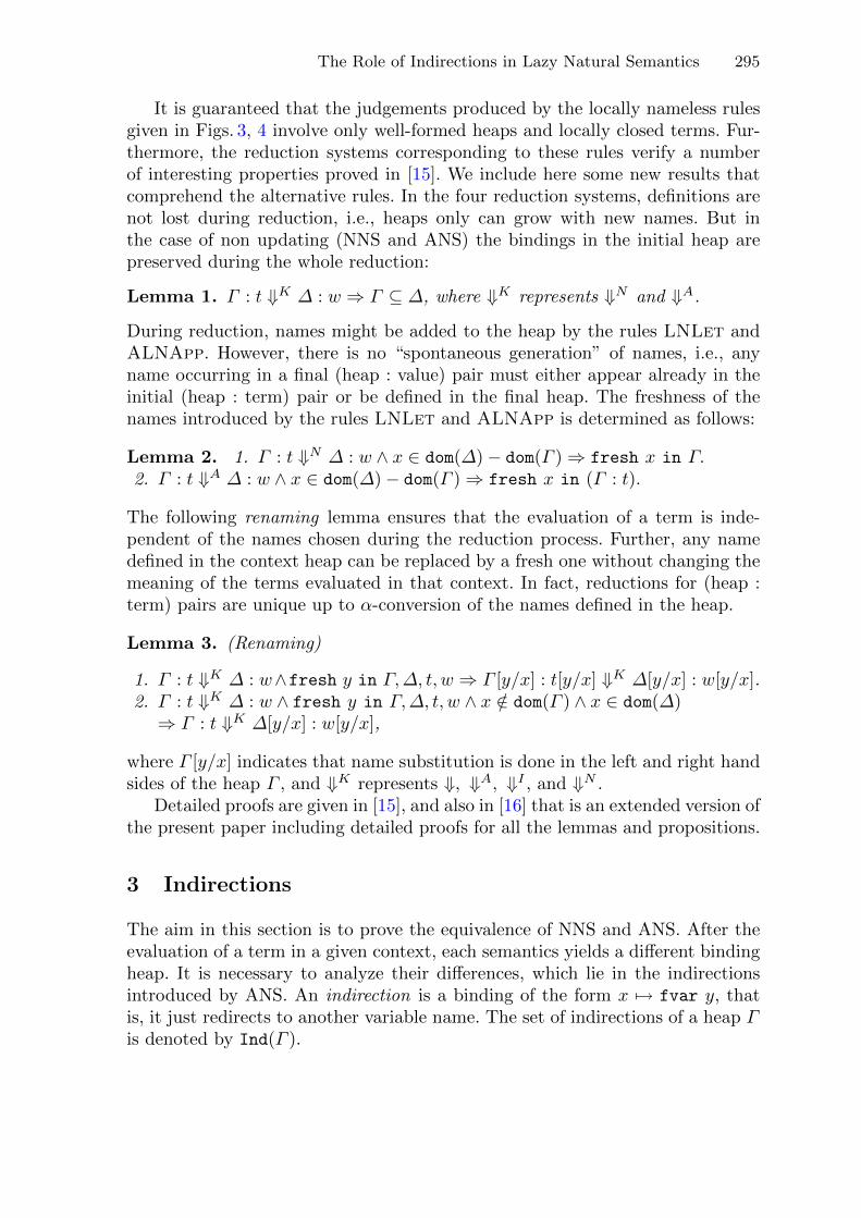
The Role of Indirections in Lazy Natural Semantics 295
It is guaranteed that the judgements produced by the locally nameless rulesgiven in Figs. 3, 4 involve only well-formed heaps and locally closed terms. Fur-thermore, the reduction systems corresponding to these rules verify a numberof interesting properties proved in [15]. We include here some new results thatcomprehend the alternative rules. In the four reduction systems, definitions arenot lost during reduction, i.e., heaps only can grow with new names. But inthe case of non updating (NNS and ANS) the bindings in the initial heap arepreserved during the whole reduction:
Lemma 1. Γ : t ⇓K Δ : w ⇒ Γ ⊆ Δ, where ⇓K represents ⇓N and ⇓A.
During reduction, names might be added to the heap by the rules LNLet andALNApp. However, there is no “spontaneous generation” of names, i.e., anyname occurring in a final (heap : value) pair must either appear already in theinitial (heap : term) pair or be defined in the final heap. The freshness of thenames introduced by the rules LNLet and ALNApp is determined as follows:
Lemma 2. 1. Γ : t ⇓N Δ : w ∧ x ∈ dom(Δ) − dom(Γ ) ⇒ fresh x in Γ.2. Γ : t ⇓A Δ : w ∧ x ∈ dom(Δ) − dom(Γ ) ⇒ fresh x in (Γ : t).
The following renaming lemma ensures that the evaluation of a term is inde-pendent of the names chosen during the reduction process. Further, any namedefined in the context heap can be replaced by a fresh one without changing themeaning of the terms evaluated in that context. In fact, reductions for (heap :term) pairs are unique up to α-conversion of the names defined in the heap.
Lemma 3. (Renaming)
1. Γ : t ⇓K Δ : w∧fresh y in Γ,Δ, t, w ⇒ Γ [y/x] : t[y/x] ⇓K Δ[y/x] : w[y/x].2. Γ : t ⇓K Δ : w ∧ fresh y in Γ,Δ, t, w ∧ x /∈ dom(Γ ) ∧ x ∈ dom(Δ)
⇒ Γ : t ⇓K Δ[y/x] : w[y/x],
where Γ [y/x] indicates that name substitution is done in the left and right handsides of the heap Γ , and ⇓K represents ⇓, ⇓A, ⇓I , and ⇓N .
Detailed proofs are given in [15], and also in [16] that is an extended version ofthe present paper including detailed proofs for all the lemmas and propositions.
3 Indirections
The aim in this section is to prove the equivalence of NNS and ANS. After theevaluation of a term in a given context, each semantics yields a different bindingheap. It is necessary to analyze their differences, which lie in the indirectionsintroduced by ANS. An indirection is a binding of the form x → fvar y, thatis, it just redirects to another variable name. The set of indirections of a heap Γis denoted by Ind(Γ ).
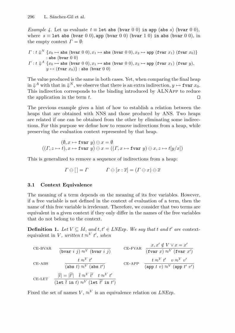
296 L. Sanchez-Gil et al.
Example 4. Let us evaluate t ≡ let abs (bvar 0 0) in app (abs s) (bvar 0 0),where s ≡ let abs (bvar 0 0), app (bvar 0 0) (bvar 1 0) in abs (bvar 0 0), inthe empty context Γ = ∅:
Γ : t ⇓N {x0 → abs (bvar 0 0), x1 → abs (bvar 0 0), x2 → app (fvar x1) (fvar x0)}: abs (bvar 0 0)
Γ : t ⇓A {x0 → abs (bvar 0 0), x1 → abs (bvar 0 0), x2 → app (fvar x1) (fvar y),y → (fvar x0)} : abs (bvar 0 0)
The value produced is the same in both cases. Yet, when comparing the final heapin ⇓A with that in ⇓N , we observe that there is an extra indirection, y → fvar x0.This indirection corresponds to the binding introduced by ALNApp to reducethe application in the term t. ��The previous example gives a hint of how to establish a relation between theheaps that are obtained with NNS and those produced by ANS. Two heapsare related if one can be obtained from the other by eliminating some indirec-tions. For this purpose we define how to remove indirections from a heap, whilepreserving the evaluation context represented by that heap.
(∅, x → fvar y) � x = ∅((Γ, z → t), x → fvar y) � x = ((Γ, x → fvar y) � x, z → t[y/x])
This is generalized to remove a sequence of indirections from a heap:
Γ � [ ] = Γ Γ � [x : x] = (Γ � x) � x
3.1 Context Equivalence
The meaning of a term depends on the meaning of its free variables. However,if a free variable is not defined in the context of evaluation of a term, then thename of this free variable is irrelevant. Therefore, we consider that two terms areequivalent in a given context if they only differ in the names of the free variablesthat do not belong to the context.
Definition 1. Let V ⊆ Id, and t, t′ ∈ LNExp. We say that t and t′ are context-equivalent in V , written t ≈V t′, when
ce-bvar(bvar i j) ≈V (bvar i j)
ce-fvarx, x′ /∈ V ∨ x = x′
(fvar x) ≈V (fvar x′)
ce-abst ≈V t′
(abs t) ≈V (abs t′)ce-app
t ≈V t′ v ≈V v′
(app t v) ≈V (app t′ v′)
ce-let|t| = |t′| t ≈V t′ t ≈V t′
(let t in t) ≈V (let t′ in t′)
Fixed the set of names V , ≈V is an equivalence relation on LNExp.
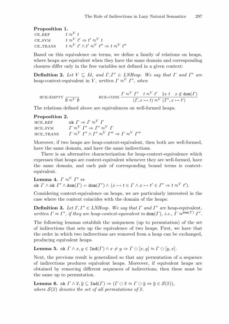
The Role of Indirections in Lazy Natural Semantics 297
Proposition 1.ce ref t ≈V tce sym t ≈V t′ ⇒ t′ ≈V tce trans t ≈V t′ ∧ t′ ≈V t′′ ⇒ t ≈V t′′
Based on this equivalence on terms, we define a family of relations on heaps,where heaps are equivalent when they have the same domain and correspondingclosures differ only in the free variables not defined in a given context:
Definition 2. Let V ⊆ Id, and Γ, Γ ′ ∈ LNHeap. We say that Γ and Γ ′ areheap-context-equivalent in V , written Γ ≈V Γ ′, when
hce-empty ∅ ≈V ∅ hce-consΓ ≈V Γ ′ t ≈V t′ lc t x /∈ dom(Γ )
(Γ, x → t) ≈V (Γ ′, x → t′)
The relations defined above are equivalences on well-formed heaps.
Proposition 2.hce ref ok Γ ⇒ Γ ≈V Γhce sym Γ ≈V Γ ′ ⇒ Γ ′ ≈V Γhce trans Γ ≈V Γ ′ ∧ Γ ′ ≈V Γ ′′ ⇒ Γ ≈V Γ ′′
Moreover, if two heaps are heap-context-equivalent, then both are well-formed,have the same domain, and have the same indirections.
There is an alternative characterization for heap-context-equivalence whichexpresses that heaps are context-equivalent whenever they are well-formed, havethe same domain, and each pair of corresponding bound terms is context-equivalent.
Lemma 4. Γ ≈V Γ ′ ⇔ok Γ ∧ ok Γ ′ ∧ dom(Γ ) = dom(Γ ′)∧ (x → t ∈ Γ ∧ x → t′ ∈ Γ ′ ⇒ t ≈V t′).
Considering context-equivalence on heaps, we are particularly interested in thecase where the context coincides with the domain of the heaps:
Definition 3. Let Γ, Γ ′ ∈ LNHeap. We say that Γ and Γ ′ are heap-equivalent,written Γ ≈ Γ ′, if they are heap-context-equivalent in dom(Γ ), i.e., Γ ≈dom(Γ ) Γ ′.
The following lemmas establish the uniqueness (up to permutation) of the setof indirections that sets up the equivalence of two heaps. First, we have thatthe order in which two indirections are removed from a heap can be exchanged,producing equivalent heaps.
Lemma 5. ok Γ ∧ x, y ∈ Ind(Γ ) ∧ x �= y ⇒ Γ � [x, y] ≈ Γ � [y, x].
Next, the previous result is generalized so that any permutation of a sequenceof indirections produces equivalent heaps. Moreover, if equivalent heaps areobtained by removing different sequences of indirections, then these must bethe same up to permutation.
Lemma 6. ok Γ ∧ x, y ⊆ Ind(Γ ) ⇒ (Γ � x ≈ Γ � y ⇔ y ∈ S(x)),where S(x) denotes the set of all permutations of x.
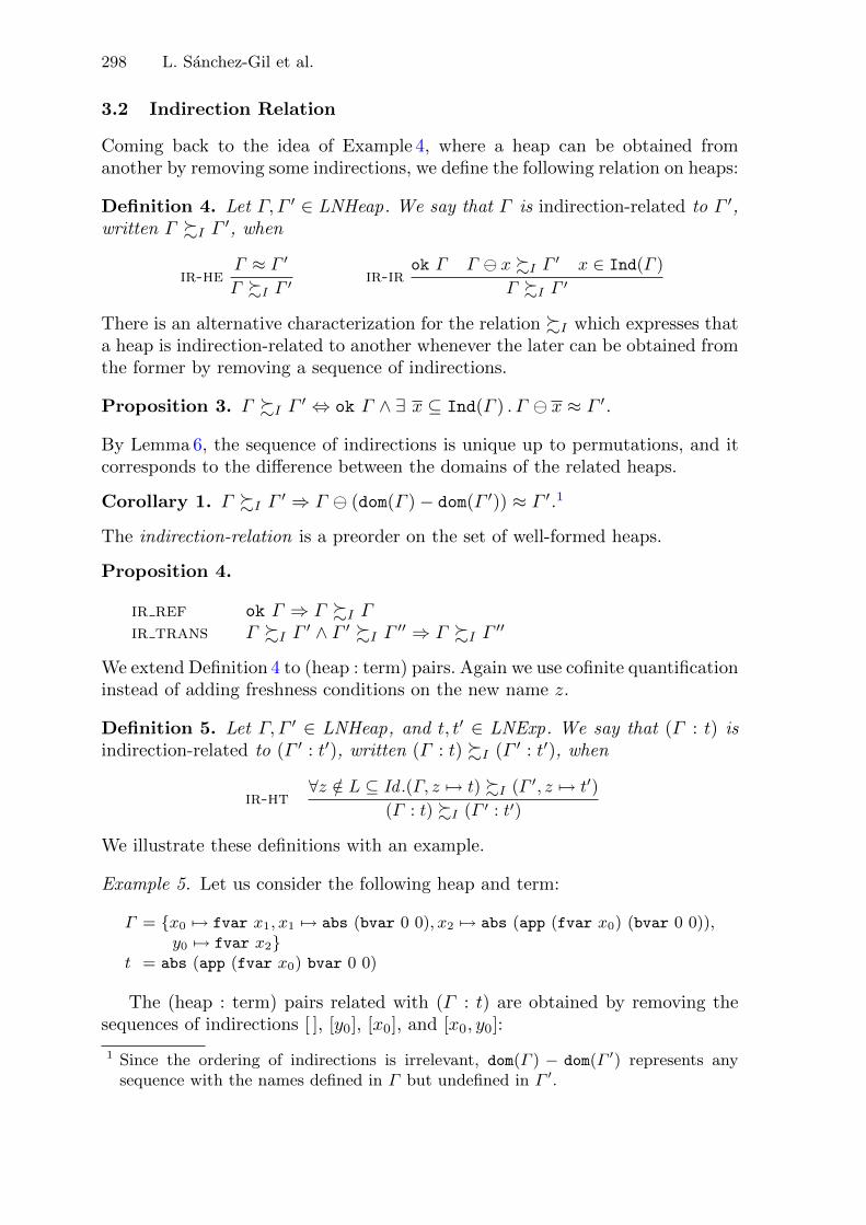
298 L. Sanchez-Gil et al.
3.2 Indirection Relation
Coming back to the idea of Example 4, where a heap can be obtained fromanother by removing some indirections, we define the following relation on heaps:
Definition 4. Let Γ, Γ ′ ∈ LNHeap. We say that Γ is indirection-related to Γ ′,written Γ �I Γ ′, when
ir-heΓ ≈ Γ ′
Γ �I Γ ′ ir-irok Γ Γ � x �I Γ ′ x ∈ Ind(Γ )
Γ �I Γ ′
There is an alternative characterization for the relation �I which expresses thata heap is indirection-related to another whenever the later can be obtained fromthe former by removing a sequence of indirections.
Proposition 3. Γ �I Γ ′ ⇔ ok Γ ∧ ∃ x ⊆ Ind(Γ ) . Γ � x ≈ Γ ′.
By Lemma 6, the sequence of indirections is unique up to permutations, and itcorresponds to the difference between the domains of the related heaps.
Corollary 1. Γ �I Γ ′ ⇒ Γ � (dom(Γ ) − dom(Γ ′)) ≈ Γ ′.1
The indirection-relation is a preorder on the set of well-formed heaps.
Proposition 4.
ir ref ok Γ ⇒ Γ �I Γir trans Γ �I Γ ′ ∧ Γ ′ �I Γ ′′ ⇒ Γ �I Γ ′′
We extend Definition 4 to (heap : term) pairs. Again we use cofinite quantificationinstead of adding freshness conditions on the new name z.
Definition 5. Let Γ, Γ ′ ∈ LNHeap, and t, t′ ∈ LNExp. We say that (Γ : t) isindirection-related to (Γ ′ : t′), written (Γ : t) �I (Γ ′ : t′), when
ir-ht∀z /∈ L ⊆ Id .(Γ, z → t) �I (Γ ′, z → t′)
(Γ : t) �I (Γ ′ : t′)
We illustrate these definitions with an example.
Example 5. Let us consider the following heap and term:
Γ = {x0 → fvar x1, x1 → abs (bvar 0 0), x2 → abs (app (fvar x0) (bvar 0 0)),y0 → fvar x2}
t = abs (app (fvar x0) bvar 0 0)
The (heap : term) pairs related with (Γ : t) are obtained by removing thesequences of indirections [ ], [y0], [x0], and [x0, y0]:
1 Since the ordering of indirections is irrelevant, dom(Γ ) − dom(Γ ′) represents anysequence with the names defined in Γ but undefined in Γ ′.
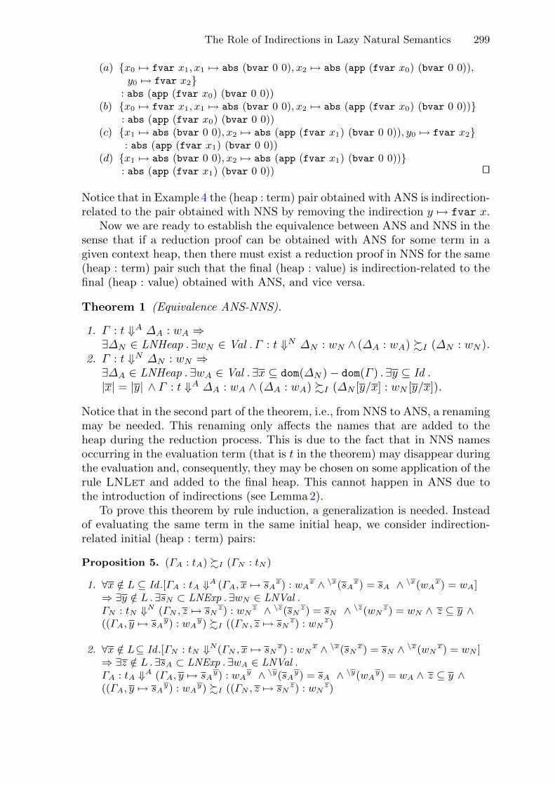
The Role of Indirections in Lazy Natural Semantics 299
(a) {x0 → fvar x1, x1 → abs (bvar 0 0), x2 → abs (app (fvar x0) (bvar 0 0)),y0 → fvar x2}
: abs (app (fvar x0) (bvar 0 0))(b) {x0 → fvar x1, x1 → abs (bvar 0 0), x2 → abs (app (fvar x0) (bvar 0 0))}
: abs (app (fvar x0) (bvar 0 0))(c) {x1 → abs (bvar 0 0), x2 → abs (app (fvar x1) (bvar 0 0)), y0 → fvar x2}
: abs (app (fvar x1) (bvar 0 0))(d) {x1 → abs (bvar 0 0), x2 → abs (app (fvar x1) (bvar 0 0))}
: abs (app (fvar x1) (bvar 0 0)) ��
Notice that in Example 4 the (heap : term) pair obtained with ANS is indirection-related to the pair obtained with NNS by removing the indirection y → fvar x.
Now we are ready to establish the equivalence between ANS and NNS in thesense that if a reduction proof can be obtained with ANS for some term in agiven context heap, then there must exist a reduction proof in NNS for the same(heap : term) pair such that the final (heap : value) is indirection-related to thefinal (heap : value) obtained with ANS, and vice versa.
Theorem 1 (Equivalence ANS-NNS).
1. Γ : t ⇓A ΔA : wA ⇒∃ΔN ∈ LNHeap .∃wN ∈ Val . Γ : t ⇓N ΔN : wN ∧ (ΔA : wA) �I (ΔN : wN ).
2. Γ : t ⇓N ΔN : wN ⇒∃ΔA ∈ LNHeap .∃wA ∈ Val .∃x ⊆ dom(ΔN ) − dom(Γ ) .∃y ⊆ Id .|x| = |y| ∧ Γ : t ⇓A ΔA : wA ∧ (ΔA : wA) �I (ΔN [y/x] : wN [y/x]).
Notice that in the second part of the theorem, i.e., from NNS to ANS, a renamingmay be needed. This renaming only affects the names that are added to theheap during the reduction process. This is due to the fact that in NNS namesoccurring in the evaluation term (that is t in the theorem) may disappear duringthe evaluation and, consequently, they may be chosen on some application of therule LNLet and added to the final heap. This cannot happen in ANS due tothe introduction of indirections (see Lemma 2).
To prove this theorem by rule induction, a generalization is needed. Insteadof evaluating the same term in the same initial heap, we consider indirection-related initial (heap : term) pairs:
Proposition 5. (ΓA : tA) �I (ΓN : tN )
1. ∀x /∈ L ⊆ Id .[ΓA : tA ⇓A (ΓA, x → sAx) : wA
x ∧ \x(sAx) = sA ∧ \x(wA
x) = wA]⇒ ∃y /∈ L . ∃sN ⊂ LNExp . ∃wN ∈ LNVal .ΓN : tN ⇓N (ΓN , z → sN
z) : wNz ∧ \z(sN
z) = sN ∧ \z(wNz) = wN ∧ z ⊆ y ∧
((ΓA, y → sAy) : wA
y) �I ((ΓN , z → sNz) : wN
z)
2. ∀x /∈ L⊆ Id .[ΓN : tN ⇓N(ΓN , x → sNx) : wN
x ∧ \x(sNx) = sN ∧ \x(wN
x) = wN ]⇒ ∃z /∈ L . ∃sA ⊂ LNExp . ∃wA ∈ LNVal .ΓA : tA ⇓A (ΓA, y → sA
y) : wAy ∧ \y(sA
y) = sA ∧ \y(wAy) = wA ∧ z ⊆ y ∧
((ΓA, y → sAy) : wA
y) �I ((ΓN , z → sNz) : wN
z)

300 L. Sanchez-Gil et al.
NATURAL SEMANTICS (NS)Indirections: NoUpdate: Yes
INDIRECTED NAT. SEM. (INS)Indirections: YesUpdate: Yes
NO-UPDATED NAT. SEM. (NNS)Indirections: NoUpdate: No
ALTERNATIVE NAT. SEM. (ANS)Indirections: Yes
Update: No
I
GU
Fig. 5. The relations between the semantics
Once more, cofinite quantification replaces freshness conditions. For instance,in the second part of the proposition it is required that the names introducedduring the reduction for NNS do not collide with names that are already definedin the initial heap for ANS. The cofinite quantification expresses that if there isan infinite number of “similar” reduction proofs for (ΓN : tN ), each introducingalternative names in the heap, one can chose a reduction proof such that thenew bindings do not interfere with (ΓA : tA).
Since there is update neither in ANS nor in NNS (Lemma1), a final heap canbe expressed as the initial heap plus some set of bindings, such as (ΓA, x → sA
x).In this case, x represents the list of new names, i.e., those that have been addedduring the reduction of local declarations, as well as the indirections introducedby the alternative application rule. Since the terms bound to these new namesare dependent on x, they are represented as sA
x. Similarly for the final valuewA
x. The proposition indicates that it is possible to construct reductions forNNS whose set of new defined names is a subset of the set of new names of thecorresponding ANS reduction (NNS only adds new names with the rule LNLet).Detailed proofs of the theorem and the proposition are given in [16].
4 Conclusions and Future Work
Launchbury natural semantics (NS) has turned out to be too much sensitiveto the changes introduced by the alternative semantics (ANS), i.e., indirectionsand no-update. These changes should lead to the same values, but this cannotbe directly established since values may contain free variables which are depen-dent on the context of evaluation, represented by the heap. And, precisely, thechanges introduced by the ANS do affect deeply the heaps. In fact, the equiva-lence of the values produced by the NS and the ANS is based on their correctnesswith respect to a denotational semantics. Although indirections and duplicatedbindings (consequence of not updating) do not add new information to the heap,it is not straightforward to prove it formally.
Since the variations introduced by Launchbury in the ANS do affect tworules, i.e. the variable rule (no-update) and the application rule (indirections),
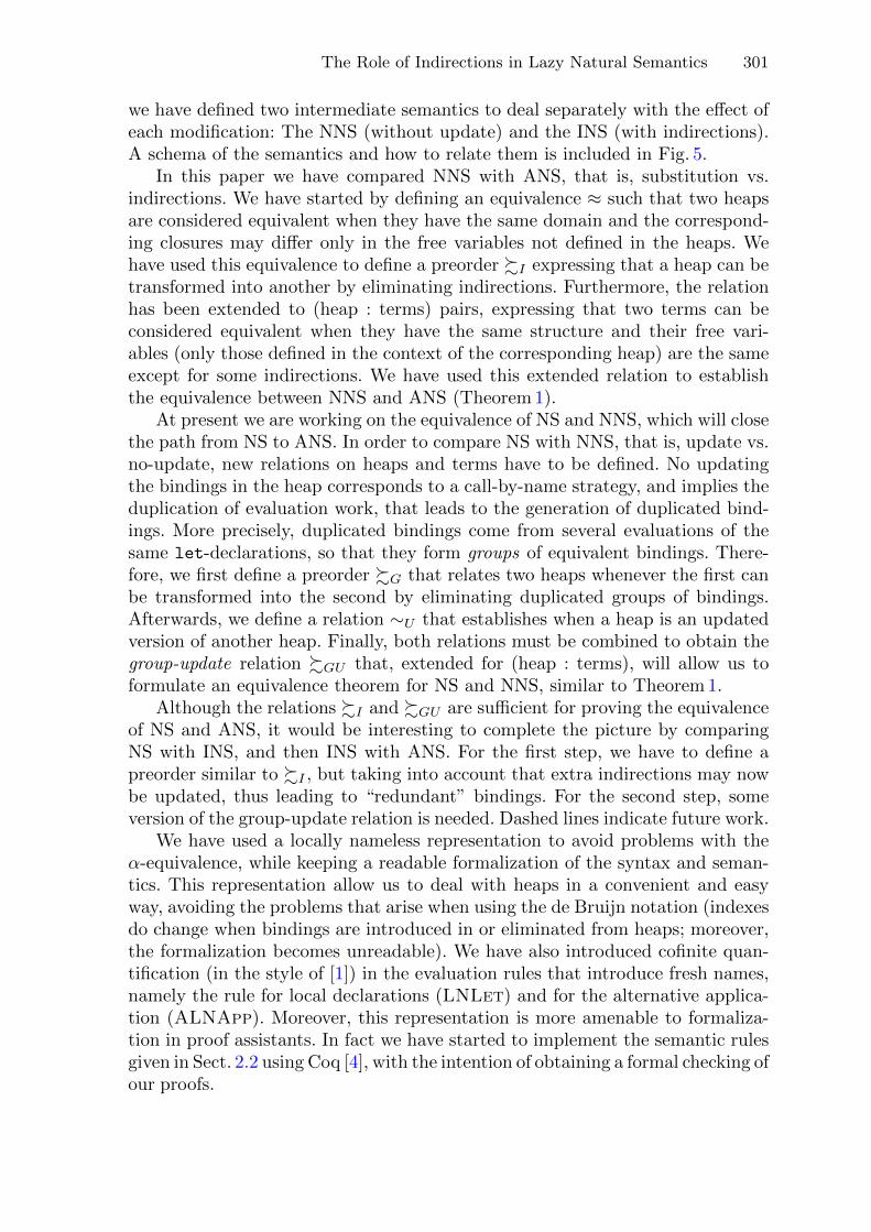
The Role of Indirections in Lazy Natural Semantics 301
we have defined two intermediate semantics to deal separately with the effect ofeach modification: The NNS (without update) and the INS (with indirections).A schema of the semantics and how to relate them is included in Fig. 5.
In this paper we have compared NNS with ANS, that is, substitution vs.indirections. We have started by defining an equivalence ≈ such that two heapsare considered equivalent when they have the same domain and the correspond-ing closures may differ only in the free variables not defined in the heaps. Wehave used this equivalence to define a preorder �I expressing that a heap can betransformed into another by eliminating indirections. Furthermore, the relationhas been extended to (heap : terms) pairs, expressing that two terms can beconsidered equivalent when they have the same structure and their free vari-ables (only those defined in the context of the corresponding heap) are the sameexcept for some indirections. We have used this extended relation to establishthe equivalence between NNS and ANS (Theorem 1).
At present we are working on the equivalence of NS and NNS, which will closethe path from NS to ANS. In order to compare NS with NNS, that is, update vs.no-update, new relations on heaps and terms have to be defined. No updatingthe bindings in the heap corresponds to a call-by-name strategy, and implies theduplication of evaluation work, that leads to the generation of duplicated bind-ings. More precisely, duplicated bindings come from several evaluations of thesame let-declarations, so that they form groups of equivalent bindings. There-fore, we first define a preorder �G that relates two heaps whenever the first canbe transformed into the second by eliminating duplicated groups of bindings.Afterwards, we define a relation ∼U that establishes when a heap is an updatedversion of another heap. Finally, both relations must be combined to obtain thegroup-update relation �GU that, extended for (heap : terms), will allow us toformulate an equivalence theorem for NS and NNS, similar to Theorem1.
Although the relations �I and �GU are sufficient for proving the equivalenceof NS and ANS, it would be interesting to complete the picture by comparingNS with INS, and then INS with ANS. For the first step, we have to define apreorder similar to �I , but taking into account that extra indirections may nowbe updated, thus leading to “redundant” bindings. For the second step, someversion of the group-update relation is needed. Dashed lines indicate future work.
We have used a locally nameless representation to avoid problems with theα-equivalence, while keeping a readable formalization of the syntax and seman-tics. This representation allow us to deal with heaps in a convenient and easyway, avoiding the problems that arise when using the de Bruijn notation (indexesdo change when bindings are introduced in or eliminated from heaps; moreover,the formalization becomes unreadable). We have also introduced cofinite quan-tification (in the style of [1]) in the evaluation rules that introduce fresh names,namely the rule for local declarations (LNLet) and for the alternative applica-tion (ALNApp). Moreover, this representation is more amenable to formaliza-tion in proof assistants. In fact we have started to implement the semantic rulesgiven in Sect. 2.2 using Coq [4], with the intention of obtaining a formal checking ofour proofs.

302 L. Sanchez-Gil et al.
Acknowledgments. This work is partially supported by the projects: TIN2012-39391-C04-04 and S2009/TIC-1465.
References
1. Aydemir, B.E., Chargueraud, A., Pierce, B.C., Pollack, R., Weirich, S.: Engineeringformal metatheory. In: ACM Symposium on Principles of Programming Languages,POPL 2008, pp. 3–15. ACM Press (2008)
2. Baker-Finch, C., King, D., Trinder, P.W.: An operational semantics for parallellazy evaluation. In: ACM-SIGPLAN International Conference on Functional Pro-gramming (ICFP 2000), Montreal, Canada, pp. 162–173, September 2000
3. Barendregt, H.P.: The Lambda Calculus: Its Syntax and Semantics. Studies inLogic and the Foundations of Mathematics, vol. 103. North-Holland, Amsterdam(1984)
4. Bertot, Y.: Coq in a hurry. CoRR, abs/cs/0603118 (2006)5. Breitner, J.: The correctness of launchbury’s natural semantics for lazy evaluation.
Archive of Formal Proofs, January 2013. Formal proof development, Amendedversion May 2014. http://afp.sf.net/entries/Launchbury.shtml
6. Chargueraud, A.: The locally nameless representation. J. Autom. Reason. 46(3),363–408 (2012)
7. de Bruijn, N.G.: Lambda calculus notation with nameless dummies, a tool forautomatic formula manipulation, with application to the Church-Rosser theorem.Indag. Math. 75(5), 381–392 (1972)
8. Hidalgo-Herrero, M., Ortega-Mallen, Y.: An operational semantics for the paral-lel language Eden. Parallel Process. Lett. (World Scientific Publishing Company)12(2), 211–228 (2002)
9. Launchbury, J.: A natural semantics for lazy evaluation. In: ACM Symposiumon Principles of Programming Languages, POPL 1993, pp. 144–154. ACM Press(1993)
10. Nakata, K., Hasegawa, M.: Small-step and big-step semantics for call-by-need. J.Funct. Program. 19(6), 699–722 (2009)
11. Nipkow, T., Paulson, L.C., Wenzel, M.: Isabelle/HOL. LNCS, vol. 2283. Springer,Heidelberg (2002)
12. Sanchez-Gil, L., Hidalgo-Herrero, M., Ortega-Mallen, Y.: Call-by-need, call-by-name, and natural semantics. Technical report UU-CS-2010-020, Department ofInformation and Computing Sciences, Utrech University (2010)
13. Sanchez-Gil, L., Hidalgo-Herrero, M., Ortega-Mallen, Y.: An operational semanticsfor distributed lazy evaluation. In: Trends in Functional Programming, pp. 65–80,vol. 10. Intellect (2010)
14. Sanchez-Gil, L., Hidalgo-Herrero, M., Ortega-Mallen, Y.: A locally nameless rep-resentation for a natural semantics for lazy evaluation. Technical report 01/12,Dpt. Sistemas Informaticos y Computacion. Univ. Complutense de Madrid (2012).http://federwin.sip.ucm.es/sic/investigacion/publicaciones/pdfs/SIC-1-12.pdf
15. Sanchez-Gil, L., Hidalgo-Herrero, M., Ortega-Mallen, Y.: A locally namelessrepresentation for a natural semantics for lazy evaluation. In: Roychoudhury,A., D’Souza, M. (eds.) ICTAC 2012. LNCS, vol. 7521, pp. 105–119. Springer,Heidelberg (2012)

The Role of Indirections in Lazy Natural Semantics 303
16. Sanchez-Gil, L., Hidalgo-Herrero, M., Ortega-Mallen, Y.: The role of indirectionsin lazy natural semantics (extended version). Technical report 13/13, Dpt. Sis-temas Informaticos y Computacion. Univ. Complutense de Madrid (2013). http://federwin.sip.ucm.es/sic/investigacion/publicaciones/pdfs/TR-13-13.pdf
17. Sestoft, P.: Deriving a lazy abstract machine. J. Funct. Program. 7(3), 231–264(1997)
18. Urban, C., Berghofer, S., Norrish, M.: Barendregt’s variable convention in ruleinductions. In: Pfenning, F. (ed.) CADE 2007. LNCS (LNAI), vol. 4603, pp. 35–50. Springer, Heidelberg (2007)
19. Urban, C., Kaliszyk, C.: General bindings and alpha-equivalence in nominalIsabelle. Log. Methods Comput. Sci. 8(2:14), 1–35 (2012)
20. van Eekelen, M., de Mol, M.: Proving lazy folklore with mixed lazy/strict seman-tics. In: Barendsen, E., Capretta, V., Geuvers, H., Niqui, M. (eds.) Reflectionson Type Theory, λ-calculus, and the Mind. Essays dedicated to Henk Barendregton the Occasion of his 60th Birthday, pp. 87–101. Radboud University Nijmegen(2007)
Chapter 8
An Operational Semantics forDistributed Lazy EvaluationLidia Sanchez-Gil, Mercedes Hidalgo-Herrero, Yolanda Ortega-Mallen1Category: Research
Abstract: We present a semantic model for distributed lazy evaluationwhereparallelism overrides laziness in terms of eager process creation and value com-munication. A small-step operational semantics defined with two transition levels:local rules for the internal behavior of each process, and global rules for processcreation, interaction, and scheduling. This semantics is proved to be correct andcomputational adequate with respect to a standard denotational semantics. To ob-tain these results two intermediate semantics are defined: a1-processor versionof the small-step operational semantics and an extension ofthe natural semanticsdefined in [9].
8.1 INTRODUCTION
The increase of processors speed is reaching its limit, and other ways have to beexplored to satisfy the voracity of computer applications.A promising alternativeis computing in parallel. Parallel (and concurrent) programming is not certainly anovelty, but the low costs of computer components have contributed to the prolif-eration of parallel and distributed machines. Languages that ease the complex jobof parallel programming are needed, and the functional paradigm is claimed to bea good candidate on account of its well-known advantages, such as abstraction,expressiveness, referential transparency, and a clean semantic model.
Referential transparency permits the implementation of alternative orders ofexecution while retaining the functionality of a program. This property, inherentto pure functional languages, is a key factor for the exploitation of parallelism in
1Universidad Complutense de Madrid, Spain;[email protected],[email protected], [email protected]
1
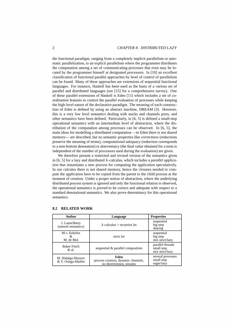
2 CHAPTER 8. DISTRIBUTED LAZY
the functional paradigm, ranging from a completely implicit parallelism or auto-matic parallelization, to an explicit parallelism where the programmer distributesthe computation among a set of communicating processes thateven may be lo-cated by the programmer himself at designated processors. In [10] an excellentclassification of functional parallel approaches by level of control of parallelismcan be found. Many of these approaches are extensions of sequential functionallanguages. For instance, Haskell has been used as the basis of a various set ofparallel and distributed languages (see [15] for a comprehensive survey). Oneof these parallel extensions of Haskell is Eden [11] which includes a set ofco-ordination features to control the parallel evaluation of processes while keepingthe high-level nature of the declarative paradigm. The meaning of each construc-tion of Eden is defined by using an abstract machine, DREAM [3]. However,this is a very low level semantics dealing with stacks and channels ports, andother semantics have been defined. Particularly, in [6, 5] isdefined a small-stepoperational semantics with an intermediate level of abstraction, where the dis-tribution of the computation among processes can be observed. In [6, 5], themain ideas for modelling a distributed computation —in Edenthere is not sharedmemory— are described, but no semantic properties likecorrectness(reductionspreserve the meaning of terms),computational adequacy(reduction correspondsto a non-bottom denotation) ordeterminacy(the final value obtained for a term isindependent of the number of processors used during the evaluation) are given.
We therefore present a restricted and revised version of thesemantics givenin [6, 5] for a lazy and distributedλ -calculus, which includes aparallel applica-tion that instantiates a new process for computing the application speculatively.In our calculus there is not shared memory, hence the closures needed to com-pute the application have to be copied from the parent to the child process at themoment of creation. Under a proper notion of abstraction, where the underlyingdistributed process system is ignored and only the functional relation is observed,the operational semantics is proved to be correct and adequate with respect to astandard denotational semantics. We also prove determinacy for this operationalsemantics.
8.2 RELATED WORK
Author Language Properties
J. Launchbury(natural semantics) λ -calculus + recursive let
sequentialbig stepsharing
M.v. Eekelen&
M. de Molstrict let
sequentialbig stepmix strict/lazy
Baker Finch& al. sequential & parallel composition
parallel threadssmall stepmix strict/lazy
M. Hidalgo-Herrero& Y. Ortega-Mallen
Edenprocess creation, dynamic channels,
no determinism, streams
several processessmall stepeager/lazy

8.3. DISTRIBUTED MODEL 3
SH1
main 7→ Ex1
1 7→ E11
x12 7→ E1
2· · ·
H2x2
1 7→ E21
x22 7→ E2
2x2
3 7→ E23
· · ·· · ·
Hnxn
1 7→ En1
xn2 7→ En
2xn
3 7→ En3
· · ·
FIGURE 8.1. A distributed model
Pz 7→ x#y −→
Pz 7→ oi 7→ y
6o?i
Co 7→ x y′
y′ 7→ i
FIGURE 8.2. Process creation
The operational semantics for Eden of [6, 5] is inspired by anoperational se-mantics for GpH [14] presented in [2]. In that work, labelledheaps are introducedto consider bindings as parallel threads. They also have twokinds of rules: sin-gle thread and multi-thread transitions, that relate roughly to our local and globaltransitions, respectively. In GPH there is no notion of independent process, andparallelism is reduced to sparkling threads in a common memory. This impliesthat there are not communications either. Besides, it is notnecessary to copybindings from one process to another. Hence, their model is much simpler thanours. Correctness, adequacy and determinacy are proved forthe operational se-mantics of GPH in [2]. We are much indebted to this work: borrowing the mainideas that are used for their proofs, and adapting them to ourcase. Our task is notonly complicated by the distributed memory, but also by the eagerness in creatingprocesses and evaluating communications.
In order to favor parallelism, Eden overrides Haskell’s laziness by creatingprocess eagerly and by forcing the evaluation of communications. The mixture oflaziness and strictness has been also investigated in the context of Launchbury’ssemantics; in [12], van Eekelen and de Mol extend the (sequential) calculus witha strict let-expression and prove the correctness and adequacy of theirmixedse-mantics.
8.3 DISTRIBUTED MODEL
Our semantic model has to reflect two features: distributionand laziness, or moreexactly, call by need. Computation is distributed among separate processes withno shared memory between them, although closures are sharedinside each pro-cess. This leads to a two-level structure (see Figure 8.1): at the top-level is adistributed system (S) with parallel processes; each process is represented at thelower-level by a heap (Hi) of bindings from variables to expressions. Heaps rep-resent the state of the computation in each process, where bindings correspondto potential concurrent threads. Thus, inside each processthere is a kind of localparallelism with shared memory.
8.3.1 The Language
We extend the calculus used in [9] (an untyped lambda calculus extended withrecursive local declarations) with aparallel applicationthat leads to process cre-

4 CHAPTER 8. DISTRIBUTED LAZY
ation. The abstract syntax is as follows:
E ::= x | λx.E | x y | x#y | let {xi = Ei}ni=1 in x
wherex,y∈ Var is the set of variables, andE ∈ EExptheextended expressions.The evaluation of a parallel applicationx#y inside a process P (the parent)
triggers the creation of a new process C (the child), and of two new channelscommunicating P and C (i and o). The parent process sends to the child thevalue for y via the input channeli, while the child process sends to its parent(through the output channelo) the result of the applicationx y. This is illustratedin Figure 8.2. There are differences with the operatorpar of GPH . First,par isjust an indication of the possibility of generating parallelism, that can be ignoredby the compiler, whereas # requires the creation of a new process even if there isonly one processor for the whole computation. Second,par generates a parallelspark that shares memory with the rest of computing threads,whereas # creates aseparate process with its own memory. Sharing between parent and child is lost,this way produce work duplication and requires some form of communicationbetween processes. # is a simplification of the process creation operator in Eden,where several input/output channels of differente types (for instance, streams withpossibly infinite sequence of data) are allowed.
Notice that our syntax is restricted, so that arguments for functional and forparallel application are variables, as the body of the let-construct. This facili-tates the definition of the operational rules, and it can be easily achieved by in-troducing new let-bindings. We also require that all variables are distinct (applyα-conversion). This restriction allows us to forget about scopes, and no garbage-collection is needed. A similar normalisation process is described by Launchburyin [9], although he only requires variables for the second argument of applications.This is insufficient for our needs2.
In the rest of the paper the following naming conventions areused:x, y, z∈Var, representing variables;i,o,ch∈ Chan, channel identifiers to model commu-nications between processes;θ , τ ∈ Var∪Chan; p, q ∈ IdProc, process identi-fiers; andW ∈ Val, values. Expressions are evaluated toweak head normal form(whnf), therefore,Val contains the terms of the formλx.E.
8.3.2 Operational Semantics
Similarly to the operational semantics presented in [2], weconsider heaps con-sisting of labelled bindingsof the form θ α7→ E, whereθ ∈ Var∪Chan, E ∈EExp∪Chan, andα ∈ {A, I ,B} is the label representing its state. A labelled bind-ing can be seen as a computation thread, which isactive(A) when being evaluated,blocked(B) when waiting for the evaluation of another binding, andinactive(I )when it has not been demanded yet or it has been already evaluated.
A labelled heap, H ∈ LHeap, is a finite set of distinct named labelled bindings.A processis a pair of the form〈p,H〉 wherep∈ IdProcandH is a labelled heap.
2In fact, in [2] the evaluation of some apparently correct expressions gets blocked.This could be easily corrected by restricting more their syntax.
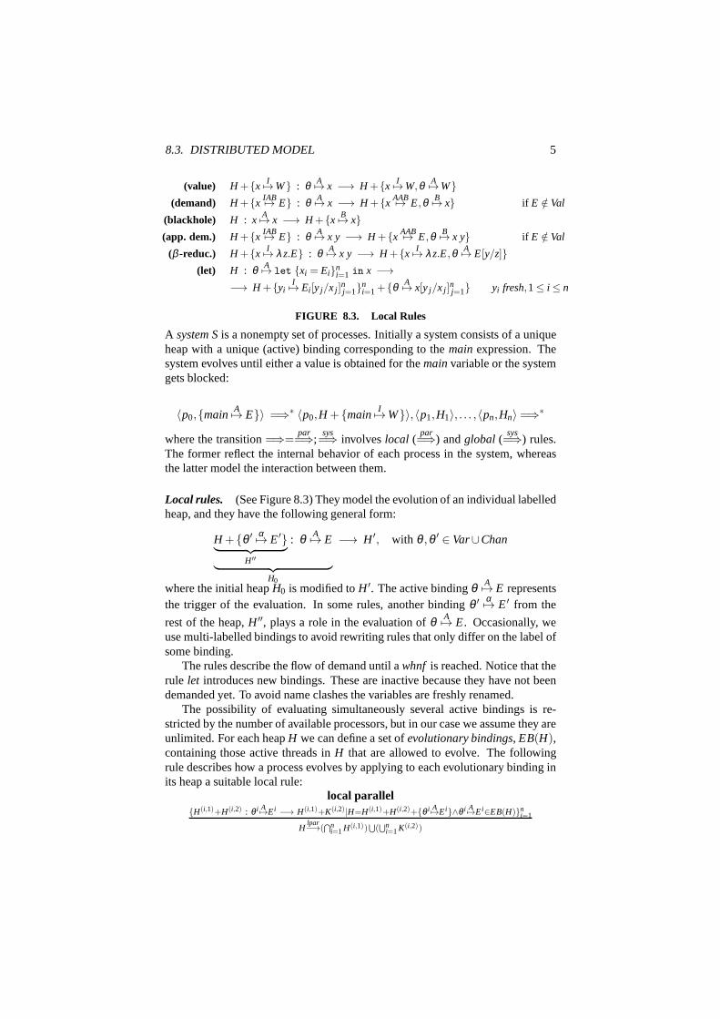
8.3. DISTRIBUTED MODEL 5
(value) H +{xI7→W} : θ A7→ x −→ H +{x
I7→W,θ A7→W}(demand) H +{x
IAB7→ E} : θ A7→ x −→ H +{xAAB7→ E,θ B7→ x} if E /∈ Val
(blackhole) H : xA7→ x −→ H +{x
B7→ x}(app. dem.) H +{x
IAB7→ E} : θ A7→ x y −→ H +{xAAB7→ E,θ B7→ x y} if E /∈ Val
(β -reduc.) H +{xI7→ λz.E} : θ A7→ x y −→ H +{x
I7→ λz.E,θ A7→ E[y/z]}(let) H : θ A7→ let {xi = Ei}n
i=1 in x −→−→ H +{yi
I7→ Ei [y j/x j ]nj=1}n
i=1 +{θ A7→ x[y j/x j ]nj=1} yi fresh,1≤ i ≤ n
FIGURE 8.3. Local Rules
A system Sis a nonempty set of processes. Initially a system consists of a uniqueheap with a unique (active) binding corresponding to themain expression. Thesystem evolves until either a value is obtained for themainvariable or the systemgets blocked:
〈p0,{mainA7→ E}〉 =⇒∗ 〈p0,H +{main
I7→W}〉,〈p1,H1〉, . . . ,〈pn,Hn〉 =⇒∗
where the transition=⇒=par=⇒;
sys=⇒ involveslocal (
par=⇒) andglobal (
sys=⇒) rules.
The former reflect the internal behavior of each process in the system, whereasthe latter model the interaction between them.
Local rules. (See Figure 8.3) They model the evolution of an individual labelledheap, and they have the following general form:
H +{θ ′ α7→ E′}︸ ︷︷ ︸H′′
: θ A7→ E
︸ ︷︷ ︸H0
−→ H ′, with θ ,θ ′ ∈ Var∪Chan
where the initial heapH0 is modified toH ′. The active bindingθ A7→ E representsthe trigger of the evaluation. In some rules, another binding θ ′ α7→ E′ from the
rest of the heap,H ′′, plays a role in the evaluation ofθ A7→ E. Occasionally, weuse multi-labelled bindings to avoid rewriting rules that only differ on the label ofsome binding.
The rules describe the flow of demand until awhnf is reached. Notice that therule let introduces new bindings. These are inactive because they have not beendemanded yet. To avoid name clashes the variables are freshly renamed.
The possibility of evaluating simultaneously several active bindings is re-stricted by the number of available processors, but in our case we assume they areunlimited. For each heapH we can define a set ofevolutionary bindings, EB(H),containing those active threads inH that are allowed to evolve. The followingrule describes how a process evolves by applying to each evolutionary binding inits heap a suitable local rule:
local parallel{H(i,1)+H(i,2) : θ i A7→Ei −→ H(i,1)+K(i,2)|H=H(i,1)+H(i,2)+{θ i A7→Ei}∧θ i A7→Ei∈EB(H)}n
i=1
Hlpar−→(
⋂ni=1H(i,1))
⋃(⋃n
i=1K(i,2))
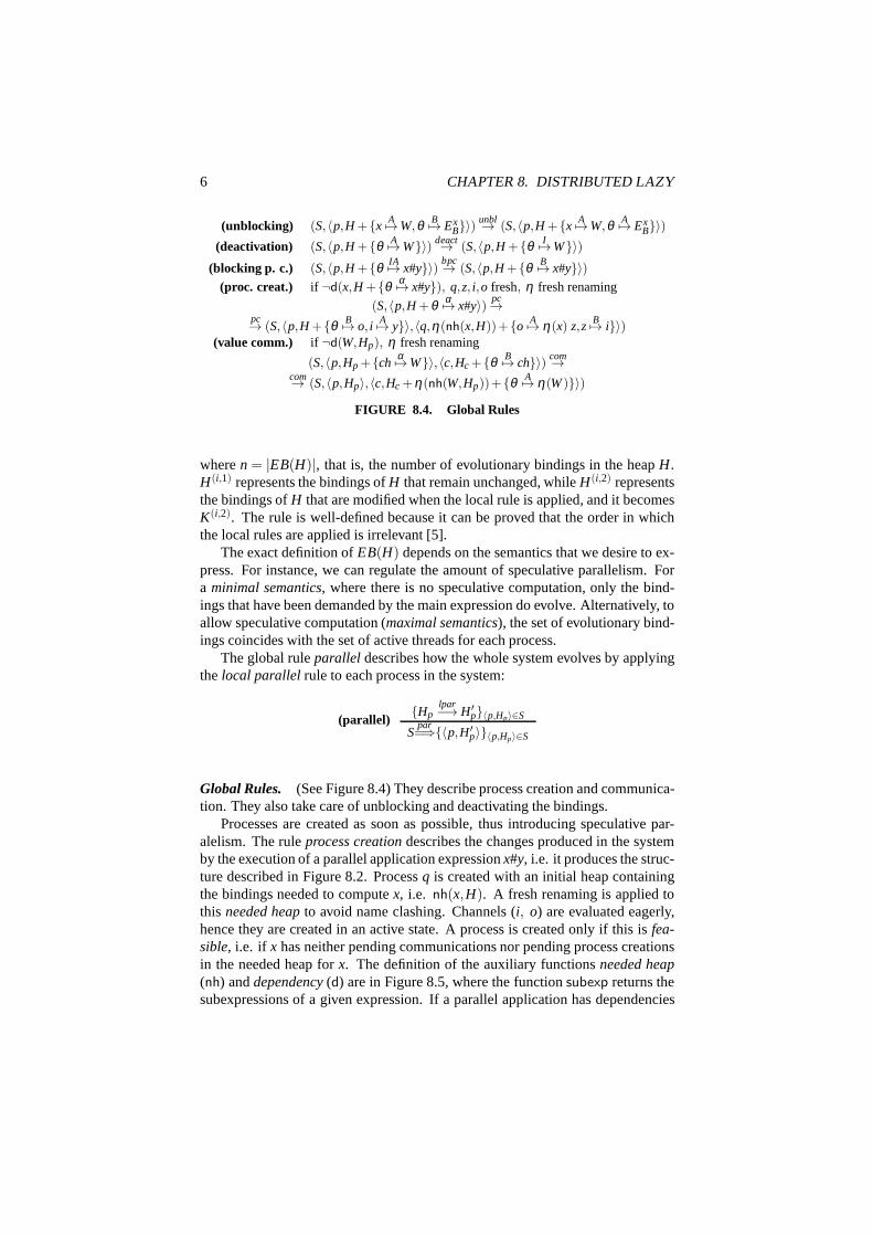
6 CHAPTER 8. DISTRIBUTED LAZY
(unblocking) (S,〈p,H +{xA7→W,θ B7→ Ex
B}〉)unbl→ (S,〈p,H +{x
A7→W,θ A7→ ExB}〉)
(deactivation) (S,〈p,H +{θ A7→W}〉) deact→ (S,〈p,H +{θ I7→W}〉)(blocking p. c.) (S,〈p,H +{θ IA7→ x#y}〉) bpc→ (S,〈p,H +{θ B7→ x#y}〉)
(proc. creat.) if ¬d(x,H +{θ α7→ x#y}), q,z, i,o fresh, η fresh renaming
(S,〈p,H +θ α7→ x#y〉) pc→pc→ (S,〈p,H +{θ B7→ o, i
A7→ y}〉,〈q,η(nh(x,H))+{oA7→ η(x) z,z
B7→ i}〉)(value comm.) if ¬d(W,Hp), η fresh renaming
(S,〈p,Hp +{chα7→W}〉,〈c,Hc +{θ B7→ ch}〉) com→
com→ (S,〈p,Hp〉,〈c,Hc +η(nh(W,Hp))+{θ A7→ η(W)}〉)
FIGURE 8.4. Global Rules
wheren = |EB(H)|, that is, the number of evolutionary bindings in the heapH.H(i,1) represents the bindings ofH that remain unchanged, whileH(i,2) representsthe bindings ofH that are modified when the local rule is applied, and it becomesK(i,2). The rule is well-defined because it can be proved that the order in whichthe local rules are applied is irrelevant [5].
The exact definition ofEB(H) depends on the semantics that we desire to ex-press. For instance, we can regulate the amount of speculative parallelism. Fora minimal semantics, where there is no speculative computation, only the bind-ings that have been demanded by the main expression do evolve. Alternatively, toallow speculative computation (maximal semantics), the set of evolutionary bind-ings coincides with the set of active threads for each process.
The global ruleparallel describes how the whole system evolves by applyingthe local parallel rule to each process in the system:
(parallel){Hp
lpar−→ H ′p}〈p,Hp〉∈S
Spar=⇒{〈p,H ′
p〉}〈p,Hp〉∈S
Global Rules. (See Figure 8.4) They describe process creation and communica-tion. They also take care of unblocking and deactivating thebindings.
Processes are created as soon as possible, thus introducingspeculative par-alelism. The ruleprocess creationdescribes the changes produced in the systemby the execution of a parallel application expressionx#y, i.e. it produces the struc-ture described in Figure 8.2. Processq is created with an initial heap containingthe bindings needed to computex, i.e. nh(x,H). A fresh renaming is applied tothis needed heapto avoid name clashing. Channels (i, o) are evaluated eagerly,hence they are created in an active state. A process is created only if this is fea-sible, i.e. if x has neither pending communications nor pending process creationsin the needed heap forx. The definition of the auxiliary functionsneeded heap(nh) anddependency(d) are in Figure 8.5, where the functionsubexp returns thesubexpressions of a given expression. If a parallel application has dependencies
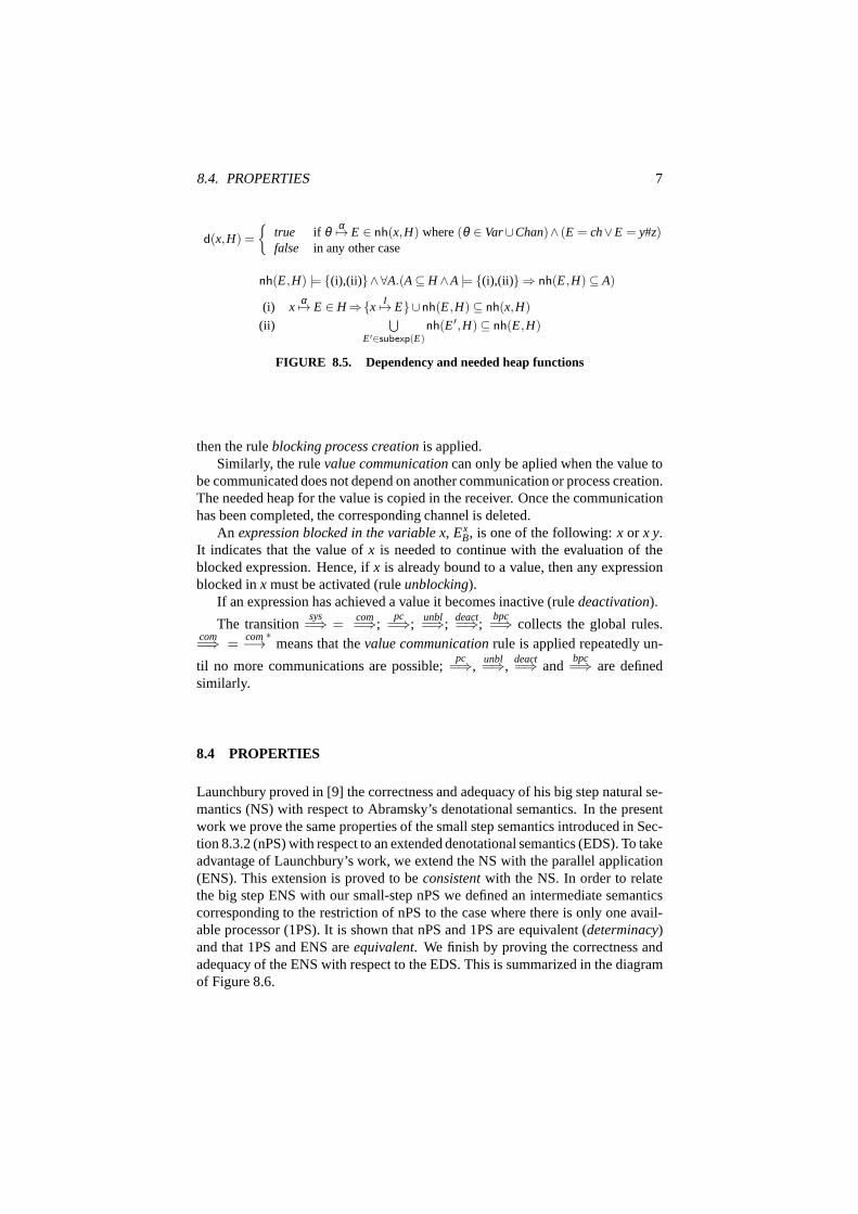
8.4. PROPERTIES 7
d(x,H) =
{true if θ α7→ E ∈ nh(x,H) where(θ ∈ Var∪Chan)∧ (E = ch∨E = y#z)false in any other case
nh(E,H) |= {(i),(ii)}∧∀A.(A⊆ H ∧A |= {(i),(ii)}⇒ nh(E,H) ⊆ A)
(i) xα7→ E ∈ H ⇒{x
I7→ E}∪nh(E,H) ⊆ nh(x,H)
(ii)⋃
E′∈subexp(E)nh(E′,H) ⊆ nh(E,H)
FIGURE 8.5. Dependency and needed heap functions
then the ruleblocking process creationis applied.Similarly, the rulevalue communicationcan only be aplied when the value to
be communicated does not depend on another communication orprocess creation.The needed heap for the value is copied in the receiver. Once the communicationhas been completed, the corresponding channel is deleted.
An expression blocked in the variable x, ExB, is one of the following:x or x y.
It indicates that the value ofx is needed to continue with the evaluation of theblocked expression. Hence, ifx is already bound to a value, then any expressionblocked inx must be activated (ruleunblocking).
If an expression has achieved a value it becomes inactive (rule deactivation).
The transitionsys
=⇒ =com=⇒;
pc=⇒;
unbl=⇒;
deact=⇒;
bpc=⇒ collects the global rules.
com=⇒ =
com−→∗means that thevalue communicationrule is applied repeatedly un-
til no more communications are possible;pc
=⇒,unbl=⇒,
deact=⇒ and
bpc=⇒ are defined
similarly.
8.4 PROPERTIES
Launchbury proved in [9] the correctness and adequacy of hisbig step natural se-mantics (NS) with respect to Abramsky’s denotational semantics. In the presentwork we prove the same properties of the small step semanticsintroduced in Sec-tion 8.3.2 (nPS) with respect to an extended denotational semantics (EDS). To takeadvantage of Launchbury’s work, we extend the NS with the parallel application(ENS). This extension is proved to beconsistentwith the NS. In order to relatethe big step ENS with our small-step nPS we defined an intermediate semanticscorresponding to the restriction of nPS to the case where there is only one avail-able processor (1PS). It is shown that nPS and 1PS are equivalent (determinacy)and that 1PS and ENS areequivalent. We finish by proving the correctness andadequacy of the ENS with respect to the EDS. This is summarized in the diagramof Figure 8.6.
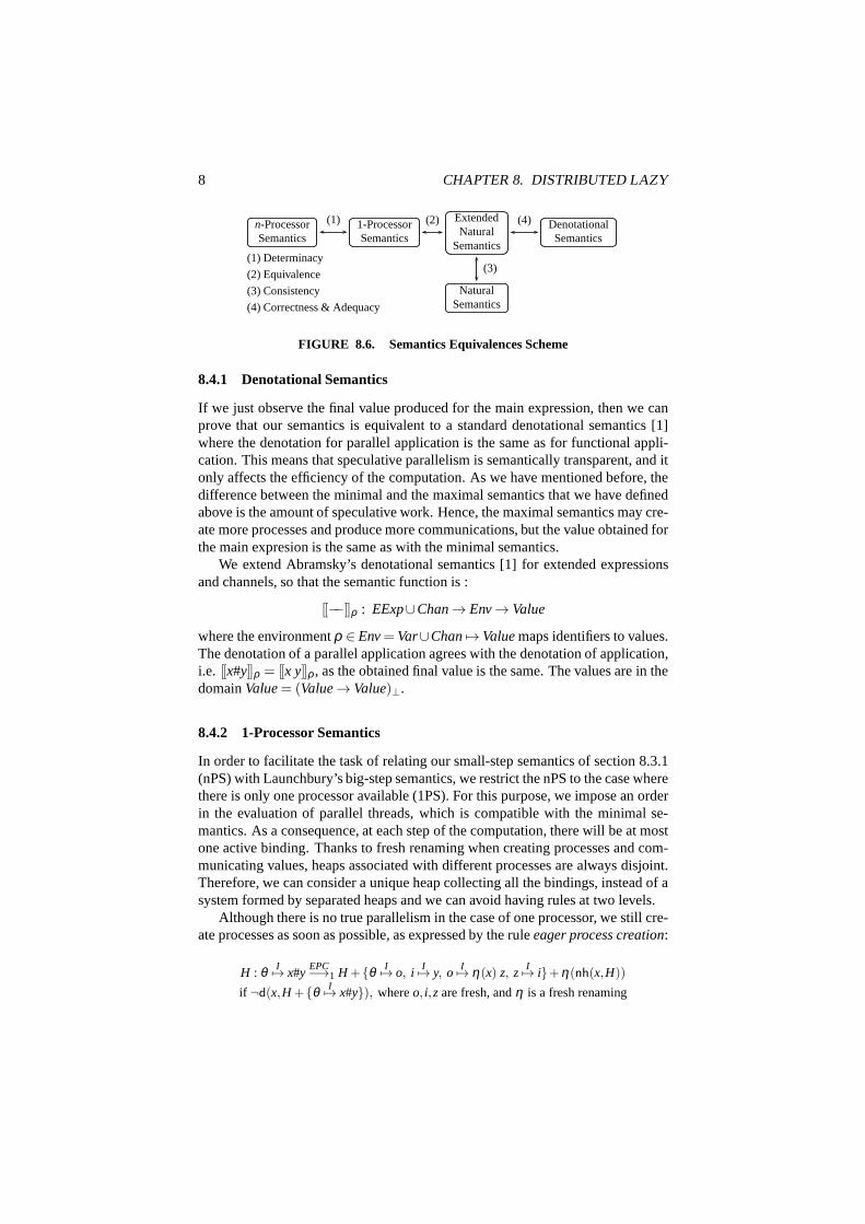
8 CHAPTER 8. DISTRIBUTED LAZY
n-ProcessorSemantics
1-ProcessorSemantics
ExtendedNatural
Semantics
NaturalSemantics
DenotationalSemantics
(1) (2)
(3)
(4)
(1) Determinacy
(2) Equivalence
(3) Consistency
(4) Correctness & Adequacy
FIGURE 8.6. Semantics Equivalences Scheme
8.4.1 Denotational Semantics
If we just observe the final value produced for the main expression, then we canprove that our semantics is equivalent to a standard denotational semantics [1]where the denotation for parallel application is the same asfor functional appli-cation. This means that speculative parallelism is semantically transparent, and itonly affects the efficiency of the computation. As we have mentioned before, thedifference between the minimal and the maximal semantics that we have definedabove is the amount of speculative work. Hence, the maximal semantics may cre-ate more processes and produce more communications, but thevalue obtained forthe main expresion is the same as with the minimal semantics.
We extend Abramsky’s denotational semantics [1] for extended expressionsand channels, so that the semantic function is :
[[−−]]ρ : EExp∪Chan→ Env→ Value
where the environmentρ ∈ Env= Var∪Chan7→ Valuemaps identifiers to values.The denotation of a parallel application agrees with the denotation of application,i.e. [[x#y]]ρ = [[x y]]ρ , as the obtained final value is the same. The values are in thedomainValue= (Value→ Value)⊥.
8.4.2 1-Processor Semantics
In order to facilitate the task of relating our small-step semantics of section 8.3.1(nPS) with Launchbury’s big-step semantics, we restrict the nPS to the case wherethere is only one processor available (1PS). For this purpose, we impose an orderin the evaluation of parallel threads, which is compatible with the minimal se-mantics. As a consequence, at each step of the computation, there will be at mostone active binding. Thanks to fresh renaming when creating processes and com-municating values, heaps associated with different processes are always disjoint.Therefore, we can consider a unique heap collecting all the bindings, instead of asystem formed by separated heaps and we can avoid having rules at two levels.
Although there is no true parallelism in the case of one processor, we still cre-ate processes as soon as possible, as expressed by the ruleeager process creation:
H : θ I7→ x#yEPC−→1 H +{θ I7→ o, i
I7→ y, oI7→ η(x) z, z
I7→ i}+η(nh(x,H))
if ¬d(x,H +{θ I7→ x#y}), whereo, i,z are fresh, andη is a fresh renaming
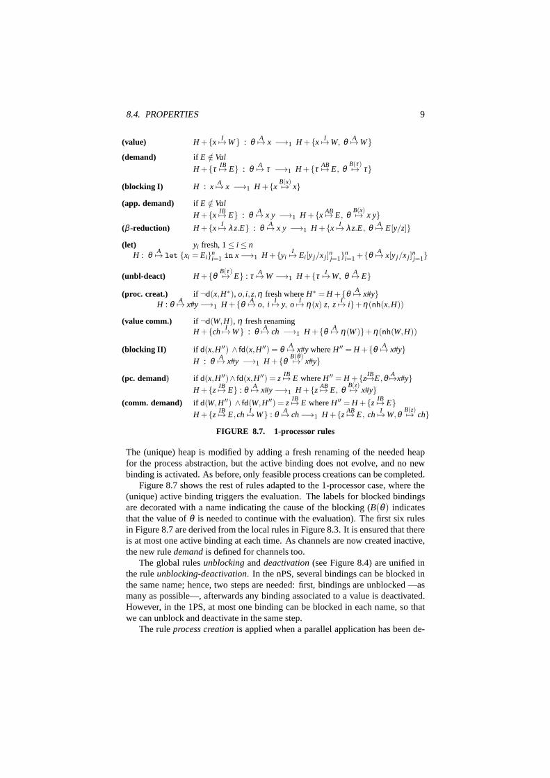
8.4. PROPERTIES 9
(value) H +{xI7→W} : θ A7→ x −→1 H +{x
I7→W, θ A7→W}(demand) if E /∈ Val
H +{τ IB7→ E} : θ A7→ τ −→1 H +{τ AB7→ E, θB(τ)7→ τ}
(blocking I) H : xA7→ x −→1 H +{x
B(x)7→ x}
(app. demand) if E /∈ Val
H +{xIB7→ E} : θ A7→ x y −→1 H +{x
AB7→ E, θB(x)7→ x y}
(β -reduction) H +{xI7→ λz.E} : θ A7→ x y −→1 H +{x
I7→ λz.E, θ A7→ E[y/z]}
(let) yi fresh, 1≤ i ≤ nH : θ A7→ let {xi = Ei}n
i=1 in x−→1 H +{yiI7→ Ei [y j/x j ]
nj=1}n
i=1 +{θ A7→ x[y j/x j ]nj=1}
(unbl-deact) H +{θB(τ)7→ E} : τ A7→W −→1 H +{τ I7→W, θ A7→ E}
(proc. creat.) if ¬d(x,H∗), o, i,z,η fresh whereH∗ = H +{θ A7→ x#y}H : θ A7→ x#y−→1 H +{θ A7→ o, i
I7→ y, oI7→ η(x) z, z
I7→ i}+η(nh(x,H))
(value comm.) if ¬d(W,H), η fresh renamingH +{ch
I7→W} : θ A7→ ch −→1 H +{θ A7→ η(W)}+η(nh(W,H))
(blocking II) if d(x,H ′′) ∧ fd(x,H ′′) = θ A7→ x#y whereH ′′ = H +{θ A7→ x#y}H : θ A7→ x#y −→1 H +{θ
B(θ)7→ x#y}
(pc. demand) if d(x,H ′′)∧ fd(x,H ′′) = zIB7→ E whereH ′′ = H +{z
IB7→E,θ A7→x#y}H +{z
IB7→ E} : θ A7→ x#y−→1 H +{zAB7→ E, θ
B(z)7→ x#y}(comm. demand) if d(W,H ′′) ∧ fd(W,H ′′) = z
IB7→ E whereH ′′ = H +{zIB7→ E}
H +{zIB7→ E,ch
I7→W} : θ A7→ ch−→1 H +{zAB7→ E, ch
I7→W,θB(z)7→ ch}
FIGURE 8.7. 1-processor rules
The (unique) heap is modified by adding a fresh renaming of theneeded heapfor the process abstraction, but the active binding does notevolve, and no newbinding is activated. As before, only feasible process creations can be completed.
Figure 8.7 shows the rest of rules adapted to the 1-processorcase, where the(unique) active binding triggers the evaluation. The labels for blocked bindingsare decorated with a name indicating the cause of the blocking (B(θ ) indicatesthat the value ofθ is needed to continue with the evaluation). The first six rulesin Figure 8.7 are derived from the local rules in Figure 8.3. It is ensured that thereis at most one active binding at each time. As channels are nowcreated inactive,the new ruledemandis defined for channels too.
The global rulesunblockinganddeactivation(see Figure 8.4) are unified inthe ruleunblocking-deactivation. In the nPS, several bindings can be blocked inthe same name; hence, two steps are needed: first, bindings are unblocked —asmany as possible—, afterwards any binding associated to a value is deactivated.However, in the 1PS, at most one binding can be blocked in eachname, so thatwe can unblock and deactivate in the same step.
The ruleprocess creationis applied when a parallel application has been de-
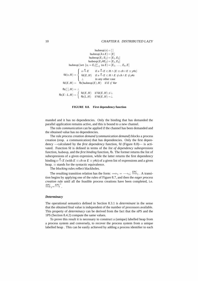
10 CHAPTER 8. DISTRIBUTED LAZY
lsubexp(x)= [ ]lsubexp(λx.E)= [E]lsubexp(E1 E2)= [E1,E2]lsubexp(E1#E2)= [E1,E2]
lsubexp(let {xi = Ei}ni=1 in E)= [E1, . . . , En,E]
fd(x,H) =
xα7→ E if x
α7→ E ∈ H ∧ (E ≡ ch∨E ≡ y#z)
fd(E,H) if xα7→ E ∈ H ∧E ≡/ ch∧E ≡/ y#z
⊥ in any other casefd(E,H) = fb(lsubexp(E),H) if E /∈ Var
fb([ ],H) = ⊥fb(E : L,H) =
{fd(E,H) if fd(E,H) 6=⊥fb(L,H) if fd(E,H) =⊥
FIGURE 8.8. First dependency function
manded and it has no dependencies. Only the binding that has demanded theparallel application remains active, and this is bound to a new channel.
The rulecommunicationcan be applied if the channel has been demanded andthe obtained value has no dependencies.
The ruleprocess creation demand(communication demand) blocks a processcreation (resp. a communication) that has dependencies. Only the first depen-dency —calculated by thefirst dependencyfunction, fd (Figure 8.8)— is acti-vated. Functionfd is defined in terms of thelist of dependency subexpresionsfunction,lsubexp, and thefirst bindingfunction,fb. The former returns the list ofsubexpresions of a given expresion, while the latter returns the first dependencybindingx
α7→ E (with E ≡ chor E ≡ y#z) of a given list of expressions and a givenheap.≡ stands for the syntactic equivalence.
Theblockingrules reflect blackholes.
The resulting transition relation has the form:=⇒1 = −→1;EPC=⇒1 . A transi-
tion begins by applying one of the rules of Figure 8.7, and then theeager processcreation rule until all the feasible process creations have been completed, i.e.EPC=⇒1=
EPC−→∗.
Determinacy
The operational semantics defined in Section 8.3.1 isdeterminantin the sensethat the obtained final value is independent of the number of processors available.This property ofdeterminacycan be derived from the fact that the nPS and the1PS (Section 8.4.2) compute the same values.
To prove this result it is necessary to construct a (unique) labelled heap froma process system and conversely, to recover the process system from a uniquelabelled heap . This can be easily achieved by adding a process identifier to each
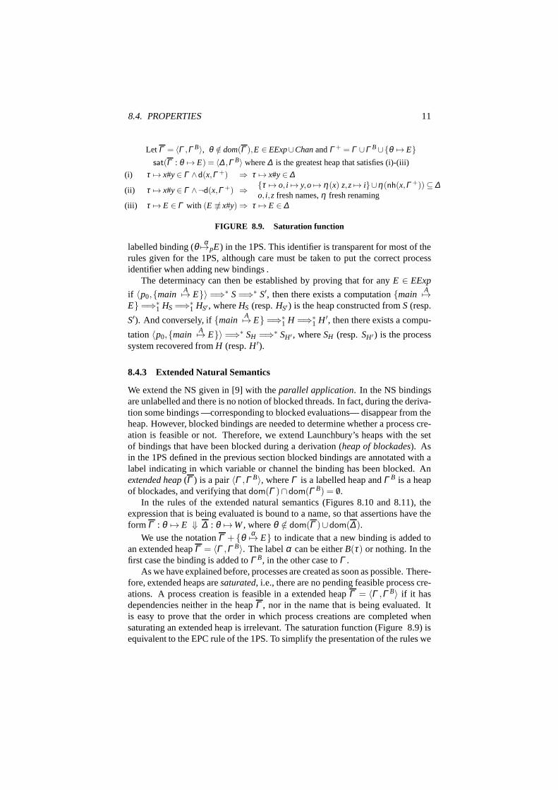
8.4. PROPERTIES 11
Let Γ = 〈Γ ,Γ B〉, θ /∈ dom(Γ ),E ∈ EExp∪ChanandΓ + = Γ ∪Γ B∪{θ 7→ E}sat(Γ : θ 7→ E) = 〈∆ ,Γ B〉 where∆ is the greatest heap that satisfies (i)-(iii)
(i) τ 7→ x#y∈ Γ ∧d(x,Γ +) ⇒ τ 7→ x#y∈ ∆
(ii) τ 7→ x#y∈ Γ ∧¬d(x,Γ +) ⇒ {τ 7→ o, i 7→ y,o 7→ η(x) z,z 7→ i}∪η(nh(x,Γ +)) ⊆ ∆o, i,z fresh names,η fresh renaming
(iii) τ 7→ E ∈ Γ with (E ≡/ x#y) ⇒ τ 7→ E ∈ ∆
FIGURE 8.9. Saturation function
labelled binding (θ α7→pE) in the 1PS. This identifier is transparent for most of therules given for the 1PS, although care must be taken to put thecorrect processidentifier when adding new bindings .
The determinacy can then be established by proving that for any E ∈ EExp
if 〈p0,{mainA7→ E}〉 =⇒∗ S=⇒∗ S′, then there exists a computation{main
A7→E} =⇒∗
1 HS =⇒∗1 HS′ , whereHS (resp.HS′ ) is the heap constructed fromS (resp.
S′). And conversely, if{mainA7→ E} =⇒∗
1 H =⇒∗1 H ′, then there exists a compu-
tation〈p0,{mainA7→ E}〉 =⇒∗ SH =⇒∗ SH′ , whereSH (resp.SH′ ) is the process
system recovered fromH (resp.H ′).
8.4.3 Extended Natural Semantics
We extend the NS given in [9] with theparallel application. In the NS bindingsare unlabelled and there is no notion of blocked threads. In fact, during the deriva-tion some bindings —corresponding to blocked evaluations—disappear from theheap. However, blocked bindings are needed to determine whether a process cre-ation is feasible or not. Therefore, we extend Launchbury’sheaps with the setof bindings that have been blocked during a derivation (heap of blockades). Asin the 1PS defined in the previous section blocked bindings are annotated with alabel indicating in which variable or channel the binding has been blocked. Anextended heap(Γ ) is a pair〈Γ ,Γ B〉, whereΓ is a labelled heap andΓ B is a heapof blockades, and verifying thatdom(Γ )∩dom(Γ B) = /0.
In the rules of the extended natural semantics (Figures 8.10and 8.11), theexpression that is being evaluated is bound to a name, so thatassertions have theform Γ : θ 7→ E ⇓ ∆ : θ 7→W, whereθ /∈ dom(Γ )∪dom(∆).
We use the notationΓ + {θ α7→ E} to indicate that a new binding is added toan extended heapΓ = 〈Γ ,Γ B〉. The labelα can be eitherB(τ) or nothing. In thefirst case the binding is added toΓ B, in the other case toΓ .
As we have explained before, processes are created as soon aspossible. There-fore, extended heaps aresaturated, i.e., there are no pending feasible process cre-ations. A process creation is feasible in a extended heapΓ = 〈Γ ,Γ B〉 if it hasdependencies neither in the heapΓ , nor in the name that is being evaluated. Itis easy to prove that the order in which process creations arecompleted whensaturating an extended heap is irrelevant. The saturation function (Figure 8.9) isequivalent to the EPC rule of the 1PS. To simplify the presentation of the rules we
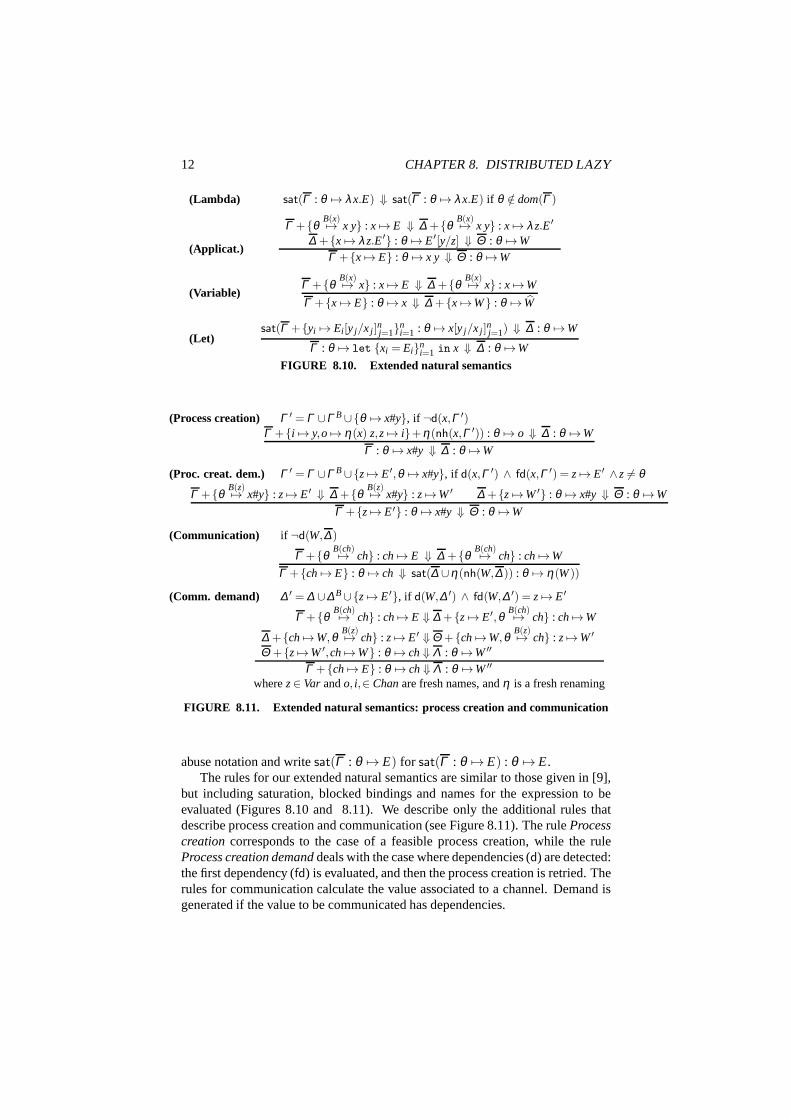
12 CHAPTER 8. DISTRIBUTED LAZY
(Lambda) sat(Γ : θ 7→ λx.E) ⇓ sat(Γ : θ 7→ λx.E) if θ /∈ dom(Γ )
(Applicat.)
Γ +{θB(x)7→ x y} : x 7→ E ⇓ ∆ +{θ
B(x)7→ x y} : x 7→ λz.E′
∆ +{x 7→ λz.E′} : θ 7→ E′[y/z] ⇓ Θ : θ 7→W
Γ +{x 7→ E} : θ 7→ x y ⇓ Θ : θ 7→W
(Variable)Γ +{θ
B(x)7→ x} : x 7→ E ⇓ ∆ +{θB(x)7→ x} : x 7→W
Γ +{x 7→ E} : θ 7→ x ⇓ ∆ +{x 7→W} : θ 7→ W
(Let)sat(Γ +{yi 7→ Ei [y j/x j ]
nj=1}n
i=1 : θ 7→ x[y j/x j ]nj=1) ⇓ ∆ : θ 7→W
Γ : θ 7→ let {xi = Ei}ni=1 in x ⇓ ∆ : θ 7→W
FIGURE 8.10. Extended natural semantics
(Process creation) Γ ′ = Γ ∪Γ B∪{θ 7→ x#y}, if ¬d(x,Γ ′)Γ +{i 7→ y,o 7→ η(x) z,z 7→ i}+η(nh(x,Γ ′)) : θ 7→ o ⇓ ∆ : θ 7→W
Γ : θ 7→ x#y ⇓ ∆ : θ 7→W
(Proc. creat. dem.) Γ ′ = Γ ∪Γ B∪{z 7→ E′,θ 7→ x#y}, if d(x,Γ ′) ∧ fd(x,Γ ′) = z 7→ E′ ∧z 6= θ
Γ +{θB(z)7→ x#y} : z 7→ E′ ⇓ ∆ +{θ
B(z)7→ x#y} : z 7→W′ ∆ +{z 7→W′} : θ 7→ x#y ⇓ Θ : θ 7→W
Γ +{z 7→ E′} : θ 7→ x#y ⇓ Θ : θ 7→W
(Communication) if ¬d(W,∆)
Γ +{θB(ch)7→ ch} : ch 7→ E ⇓ ∆ +{θ
B(ch)7→ ch} : ch 7→W
Γ +{ch 7→ E} : θ 7→ ch ⇓ sat(∆ ∪η(nh(W,∆ )) : θ 7→ η(W))
(Comm. demand) ∆ ′ = ∆ ∪∆ B∪{z 7→ E′}, if d(W,∆ ′) ∧ fd(W,∆ ′) = z 7→ E′
Γ +{θB(ch)7→ ch} : ch 7→ E ⇓ ∆ +{z 7→ E′,θ
B(ch)7→ ch} : ch 7→W
∆ +{ch 7→W,θB(z)7→ ch} : z 7→ E′ ⇓ Θ +{ch 7→W,θ
B(z)7→ ch} : z 7→W′
Θ +{z 7→W′,ch 7→W} : θ 7→ ch⇓ Λ : θ 7→W′′
Γ +{ch 7→ E} : θ 7→ ch⇓ Λ : θ 7→W′′
wherez∈ Var ando, i,∈ Chanare fresh names, andη is a fresh renaming
FIGURE 8.11. Extended natural semantics: process creation and communication
abuse notation and writesat(Γ : θ 7→ E) for sat(Γ : θ 7→ E) : θ 7→ E.The rules for our extended natural semantics are similar to those given in [9],
but including saturation, blocked bindings and names for the expression to beevaluated (Figures 8.10 and 8.11). We describe only the additional rules thatdescribe process creation and communication (see Figure 8.11). The ruleProcesscreation corresponds to the case of a feasible process creation, while the ruleProcess creation demanddeals with the case where dependencies (d) are detected:the first dependency (fd) is evaluated, and then the process creation is retried. Therules for communication calculate the value associated to achannel. Demand isgenerated if the value to be communicated has dependencies.
8.5. DISCUSSION 13
Consistency
The ENS isconsistentwith the original NS, in the sense that, if we considerexpressions without parallel application, then the same value is obtained in bothderivation systems, and the final heaps can be related, i.e. for anyE ∈ Exp wehaveΓ : E ⇓ ∆ : W iff 〈Γ ,Γ B〉 : x 7→ E ⇓ 〈∆ ,Γ B〉 : x 7→W whereΓ B is disjointfrom Γ and∆ , andx is completely a fresh variable.
Equivalence
The 1PS and the ENS are equivalent. There is an obvious conversion from labelledheaps to extended heaps (and viceversa), where inactive bindings are collected inthe first component ofΓ and blocked bindings in the second component. There-
foreH +{θ A7→ E}=⇒∗1 H ′+{θ A7→W} iff Γ : θ 7→ E ⇓ ∆ : θ 7→W whereΓ and
∆ are the extended heaps corresponding toH andH ′ respectively.
Correctness and Computational Adequacy
Following the steps given in [9], we extend the proofs forcorrectnessandcompu-tational adequacyfor the ENS respect to the EDS.
The correctness theorem establishes that the meaning of an expression doesnot change during its evaluation, and that heaps only changeby adding new bind-ings or refining the closures of the existing bindings.
Theorem 8.1 (Correctness of the ENS). Let E∈EExp∪Chan,Γ = 〈Γ ,Γ B〉, ∆ =〈∆ ,∆B〉 ∈ EHeap, andθ /∈ dom(Γ ). If Γ : θ 7→ E ⇓ ∆ : θ 7→W, then for everyenvironmentρ , [[E]]{{Γ }}ρ = [[W]]{{∆}}ρ and{{Γ}}ρ ≤ {{∆}}ρ, where the semanticfunction: {{. . .}} : Heap→ Env→ Env, defined as{{x1 7→ E1, . . . ,xn 7→ En}}ρ =µρ ′.ρ ⊔(x1 7→ [[E1]]ρ ′ . . .xn 7→ [[En]]ρ ′), beingµ the least fixed point operator, andHeap is the domain of (unlabelled) heaps, i.e. sets of unlabelled bindings. Theordering on environments is defined as in [9], so thatρ ≤ ρ ′ if ρ ′ binds morevariables thanρ .
The computational adequacy theorem states that an expression reduces to avalue if and only if its denotation is non-bottom.
Theorem 8.2 (Adequacy: of the ENS). Let E∈ EExp∪Chan,Γ = 〈Γ ,Γ B〉 ∈EHeap, andθ /∈ dom(Γ ). Γ : θ 7→ E ⇓ ∆ : θ 7→W, iff [[E]]{{Γ }}ρ 6=⊥.
8.5 DISCUSSION
Proving semantic properties like correctness or computational adequacy is muchmore than just a theoretical exercise. The search for formalproofs of these proper-ties has led to a deeper understanding of our distributed model and the interactionof distribution and parallelism with laziness. Moreover, it has revealed other inter-esting features such as how to sequentialize parallel computations and to establishan order in evaluation demand.
14 CHAPTER 8. DISTRIBUTED LAZY
For instance, our extension of Launchbury’s natural semantics could not be re-duced to adding rules for dealing with the parallel application (the only extensionin the syntax). It was necessary to add information about blocked bindings, andto saturateheaps to perform process creation eagerly.
8.6 FUTURE WORK
The syntax used in [6, 5] includes the parallel operator, andalso communicationsstreams, dynamic channels and non-determinism; an immediate future work is toextend the properties proved here to include these other features of Eden.
Although the semantic model presented here offers insightsinto the distribu-tion of computation —the systems of processes that have beencreated, and thecommunications performed during evaluation can be observed—, for correctness,adequacy and determinacy, we have just considered the final value that is calcu-lated. This relates to thevalueequivalence recently defined in [4]; in this work,three different notions of equivalence between expressions are defined. Roughly,two expressions arevalueequivalent if when they are evaluated on the same heap,the same value is obtained; they areheapequivalent if the same final heap is pro-duced (the value obtained may differ); and they arestrict equivalent if they coin-cide on the value and on the final heap. It would be interestingto investigate theseequivalences in our semantics, and to prove elementary properties for our parallelapplication as those given forseq in [4], i.e. idempotence, left-commutativityand associativity.
We are also interested in extending our results for properties beyond function-ality, like for instance work duplication, task distribution or value communica-tion, that are meaningful in a parallel and distributed context. To this purpose, theprocess system has to become part of the denotation of a program, so that pro-cess creation and communication/synchronization are side-effects produced bythe evaluation of expressions. This can be formalized by defining denotationalvalues with an additional parameter: thecontinuation, i.e., a state transformerwhich gathers the effect of the context where an expression is evaluated. Thereexists for Eden a continuation-based denotational semantics [7, 8, 5], and our ul-timate goal is to prove the equivalence between this denotational semantics andthe operational one given in [6, 5]. For this, we have to find a way to relate themechanism of continuations with that of reduction for the operational semantics.
Acknowledgements We recognise the support of the following grants: MEC:TIN2006-15660-C02-01, TIN2006-15578-C02-01 and BES-2007-16823; CAM:S-0505/TIC-0407. We thank Greg Michaelson and the anonymous referees forhis valuable comments.
REFERENCES
[1] S. Abramsky. Research Topics in Functional Programming, chapter 4: The lazylambda calculus, pages 65–117. Ed. D. A. Turner. Addison Wesley, 1990.
8.6. FUTURE WORK 15
[2] C. Baker-Finch, D. King, and P. W. Trinder. An operational semantics for parallel lazyevaluation. InACM-SIGPLAN International Conference on Functional Programming(ICFP’00), pages 162–173, Montreal, Canada, September 2000.
[3] S. Breitinger, U. Klusik, R. Loogen, Y. Ortega-Mallen,and R. Pena. DREAM –the DistRibuted Eden Abstract Machine. InProceedings of the 9th InternationalWorkshop on Implementation of Functional Languages, (IFL’97 selected papers),pages 250–269. LNCS 1467, Springer, 1997.
[4] M. J. Gabbay, S. H. Haeri, Y. Ortega-Mallen, and P. W. Trinder. Reasoning aboutselective strictness: operational equivalence, heaps andcall-by-need evaluation, newinductive principles. Insubmitted to ACM-SIGPLAN International Conference onFunctional Programming (ICFP’09), Edinburgh, UK, August 2009.
[5] M. Hidalgo-Herrero.Semanticas formales para un lenguaje funcional paralelo. PhDthesis, Dept. Sistemas Informaticos y Programacion, Universidad Complutense deMadrid, 2004.
[6] M. Hidalgo-Herrero and Y. Ortega-Mallen. An operational semantics for the parallellanguage Eden.Parallel Processing Letters (World Scientific Publishing Company),12(2):211–228, 2002.
[7] M. Hidalgo-Herrero and Y. Ortega-Mallen. Continuation semantics for parallelHaskell dialects. InProc. of the 1st Asian Symposium on Programming Languagesand Systems, pages 303–321. LNCS 2895, Springer, 2003.
[8] M. Hidalgo-Herrero and Y. Ortega-Mallen. Dealing denotationally with stream-basedcommunication.Electronic Notes in Theoretical Computer Science, 137(1):47–68,2005.
[9] J. Launchbury. A natural semantics for lazy evaluation.In ACM Symposium onPrinciples of Programming Languages, POPL’93, pages 144–154. ACM Press, 1993.
[10] R. Loogen.Research Directions in Parallel Functional Programming, chapter 3: Pro-gramming Language Constructs, pages 63–92. Eds. K. Hammondand G. Michaelson.Springer, 1999.
[11] R. Loogen, Y. Ortega-Mallen, and R. Pena. Parallel functional programming in Eden.Journal of Functional Programming, 15(3):431–475, 2005.
[12] M. van Eekelen and M. de Mol. Mixed Lazy/Strict Graph Semantics. Technicalreport, Christian-Albrechts-Universitat zu Kiel”, Technical Report 0408, 245-260,2004, Lubeck, Germany.
[13] L. Sanchez-Gil. Sobre la equivalencia entre semanticas operacionales y denota-cionales para lenguajes funcionales paralelos. Master’s thesis, Universidad Com-plutense de Madrid (Departamento de Sistemas Informaticos y Computacion), 2008.http://maude.sip.ucm.es/eden-semantics/ .
[14] P. W. Trinder, K. Hammond, H. W. Loidl, and S. L. Peyton Jones. Algorithm +Strategy = Parallelism.Journal of Funcional Programming, 8(1):23–60, 1998.
[15] P. W. Trinder, H. W. Loidl, and R. F. Pointon. Parallel and Distributed Haskells.Journal of Functional Programming, 12(4+5):469–510, 2003.

166 Capıtulo 5. Publicaciones
Apendice A
Versiones extendidas
Incluimos dos informes tecnicos (TR1 [SGHHOM12c] y TR2 [SGHHOM13]) que sonlas versiones extendidas de las publicaciones en International Colloquium on TheoreticalAspects of Computing (ICTAC’12) y Perspectives of System Informatics (PSI’14), res-pectivamente. De hecho, los tıtulos de estos artıculos coinciden con los incluidos en elCapıtulo 5: A locally nameless representation for a natural semantics for lazy evaluationy The role of indirections in lazy natural semantics. Estas versiones extendidas incluyenexplicaciones mas detalladas y todas las demostraciones, no solo de los resultados masimportantes sino tambien de todos los resultados auxiliares que han sido necesarios pararealizarlas.
We include two technical reports, (TR1 [SGHHOM12c] and TR2 [SGHHOM13]), inthis Appendix. Since they are the extended versions of the publications in InternationalColloquium on Theoretical Aspects of Computing (ICTAC’12) and Perspectives of Sys-tem Informatics (PSI’14), their titles coincide with the ones included in Chapter 5: Alocally nameless representation for a natural semantics for lazy evaluation and The roleof indirections in lazy natural semantics. These extended versions include detailed proofsof all the results.
167

168 Capıtulo A. Versiones extendidas
A locally nameless representation for a naturalsemantics for lazy evaluation
Technical Report 01/12Lidia Sanchez-Gil1, Mercedes Hidalgo-Herrero2, and Yolanda Ortega-Mallen3
1 Dpto. Sistemas Informaticos y Computacion, Facultad de CC. Matematicas,Universidad Complutense de Madrid, Spain
2 Dpto. Didactica de las Matematicas, Facultad de Educacion, UniversidadComplutense de Madrid, Spain
3 Dpto. Sistemas Informaticos y Computacion, Facultad de CC. Matematicas,Universidad Complutense de Madrid, Spain
Abstract. We propose a locally nameless representation for Launch-bury’s natural semantics for lazy evaluation. Names are reserved for freevariables, while bound variable names are replaced by indices. This avoidsthe use of α-conversion and facilitates the identification of equivalentvalues in reduction proofs. We use cofinite quantification to express thesemantic rules that introduce fresh names, but we prove that existentialrules are admissible too. Moreover, we prove that the choice of namesduring the evaluation of a term is irrelevant as long as they are freshenough.
1 Introduction
In the usual representation of the lambda-calculus, i.e., with variable namesfor free and bound variables, terms are identified up to α-conversion. This no-tation is suitable for explaining new concepts and for giving examples, whileα-substitution together with Barendregt’s variable convention [2] are freely usedin informal reasoning. But the variable convention may lead to prove false (see[8]), and α-substitution is hard to implement in an automatic proof assistant.Therefore, other representations have been proposed to avoid names and α-conversion. For instance, the de Bruijn notation [5], where variable names arereplaced by indices. However, this nameless notation is much less intuitive andquite cumbersome to use, as small modifications of a term may imply multipleshiftings of the indices. A compromise between the named representation andthe de Bruijn notation is the locally nameless representation as presented in [4].In this case, bound variable names are replaced by indices, while free variableskeep their names. This mixed notation combines the advantages of both namedand nameless representations. On the one hand, α-conversion is no longer neededand variable substitution is easily defined because there is no danger of namecapture. On the other hand, terms are still readable and easy to manipulate.
We use a locally nameless representation to express Launchbury’s naturalsemantics for lazy evaluation [6]. Our final purpose is to implement this natural

2
x ∈ Vare ∈ Exp ::= λx.e | (e x) | x | let {xi = ei}ni=1 in e.
Fig. 1. Restricted named syntax of the extended λ-calculus
semantics in some proof assistant like Coq [3], and then to prove formally severalproperties of the semantics. The reduction rule for local declarations implies theintroduction of fresh names. We use neither an existential nor a universal rulefor this case. Instead, we opt for a cofinite rule as introduced by Aydemir etal. in [1]. Nevertheless, an introduction lemma is stated (and proved) which ex-presses that an existential rule is admissible too. Our locally nameless semanticsis completed with a regularity lemma which ensures that every term and heapinvolved in a reduction proof are well-formed, and with a renaming lemma whichindicates that the choice of names (free variables) is irrelevant as long as they arefresh enough. We have experienced the advantages of using cofinite rules whendemonstrating these results.
In summary, the contributions of this paper are:
1. A locally nameless representation of the λ-calculus extended with recursivelocal declarations;
2. A locally nameless version of the inductive rules of Launchbury’s naturalsemantics for lazy evaluation;
3. A new version of cofinite rules where the variables quantified in the premisesdo appear in the conclusion too; and
4. A formal proof of several properties of our reduction system like the regu-larity, the introduction and the renaming lemmas.
The paper is structured as follows: In Section 2 we present the locally name-less representation of the lambda calculus extended with recursive local decla-rations. The locally nameless translation of the natural semantics for lazy eval-uation given in [6] is described in Section 3, together with the regularity, theintroduction and the renaming lemmas. The proofs of these lemmas and otherauxiliary results are detailed in the Appendix. In Section 4 we draw conclusionsand outline our future work.
2 The locally nameless representation
The language described in [6] is a normalized lambda calculus extended withrecursive local declarations. We reproduce the restricted syntax in Figure 1.Normalization is achieved in two steps. First an α-conversion is performed sothat all bound variables have distinct names. In a second phase, it is ensuredthat arguments for applications are restricted to be variables. These static trans-formations make more explicit the sharing of closures and, thus, simplify thedefinition of the reduction rules.
We give the corresponding locally nameless representation by following themethodology summarized in [4]:

3
x ∈ Id i, j ∈ Nv ∈ Var ::= bvar i j | fvar xt ∈ LNExp ::= v | abs t | app t v | let {ti}ni=1 in t
Fig. 2. Locally nameless syntax
1. Define the syntax of the extended λ-calculus in the locally nameless style.2. Define the variable opening and variable closing operations.3. Define the free variables and substitution functions, as well as the local
closure predicate.4. State and prove the properties of the operations on terms that are needed
in the development to be carried out.
2.1 Locally nameless syntax
The locally nameless (restricted) syntax is shown in Figure 2. Var stands nowfor the set of variables, where it is distinguished between bound variables andfree variables. The calculus includes two variable binders: λ-abstraction and let-expression. Since let declarations are multibinders, bound variables are repre-sented with two natural numbers: the first number indicates to which binderof the term (either abstraction or let) the variable is bound, while the secondrefers to the position of the variable inside the binder (in the case of an abstrac-tion this second number should be 0). In the following, we will represent a listlike {ti}ni=1 as t, with length |t| = n.
Example 1. Let e ∈ Exp be the λ-expression given in the named representation
e ≡ λz.let {x1 = λy1.y1, x2 = λy2.y2} in (z x2).
The corresponding locally nameless term t ∈ LNExp is:
t ≡ abs (let {abs (bvar 0 0), abs (bvar 0 0)} in app (bvar 1 0) (bvar 0 1)).
Notice that x1 and x2 denote α-equivalent expressions in e. This is more clearlyseen in t, where both expressions are represented with syntactically equal terms.
utApplication arguments are still restricted to variables, but the first phase
of the normalization (described at the beginning of the section) is no longerneeded.
2.2 Variable opening and variable closing
Variable opening and variable closing are the main operations to manipulate lo-cally nameless terms. We extend the definitions given in [4] to the let-expressiondefined in Figure 2.4
4 Multiple binders are defined in [4]. One corresponds to non recursive local declara-tions, and the other to mutually recursive expressions. Both constructions are treatedas extensions, so that they are not completely developed.

4
{k → x}(bvar i j) =
{fvar (List.nth j x) if i = k ∧ j < |x|bvar i j otherwise
{k → x}(fvar x) = fvar x{k → x}(abs t) = abs ({k + 1→ x} t){k → x}(app t v) = app ({k → x} t) ({k → x} v){k → x}(let t in t) = let ({k + 1→ x} t) in ({k + 1→ x} t)
where {k → x} t = List.map ({k → x} ·) t.
Fig. 3. Variable opening
In order to be able to explore the body of a binder construction (abstractionor let), one needs to replace the corresponding bound variables by fresh names.In the case of an abstraction abs t the variable opening operation provides a(fresh) name to replace in t the bound variables referring to the outermost ab-straction. Analogously, the opening of a let-term let t in t provides a list ofdistinct fresh names (as many as local declarations in t) to replace the boundvariables occurring in t and in the body t that refer to this particular declaration.
Variable opening is defined in terms of a recursive function {k → x}t (Fig-ure 3), where the number k represents the nesting level of the binder of interest,and x is a list of pairwise-distinct identifiers in Id . Since the level of the outer-most binder is 0, variable opening is defined as:
tx = {0→ x}t.
Sometimes we are interested in applying the opening operation to a list of
terms: tx
= List.map (·x) t.
The last definition and those in Figure 3 include some operations on lists.We use an ML-like notation. For instance, List.nth j x represents the (j + 1)th
element of x,5 and List.map f t indicates that the function f is applied to everyterm in the list t. In the rest of definitions we will use similar list operations.
Inversely to variable opening, there is an operation to transform free namesinto bound variables. The variable closing of a term is represented by \xt, wherex is the list of names to be bound (recall that all names in x are different). Thedefinition of variable closing is based on a recursive function {k ← x}t (Figure 4),where k indicates again the level of nesting of binders.Whenever a free variablefvar x is encountered, x is looked up in x. If x occurs in position j, then thefree variable is replaced by the bound variable (bvar k j), otherwise it is leftunchanged.Variable closing is then defined as follows:
\xt = {0← x}t.
Variable closing of a list of terms is: \xt = List.map (\x·) t.5 In order to better accommodate to bound variables indices, elements in a list are
numbered starting with 0.
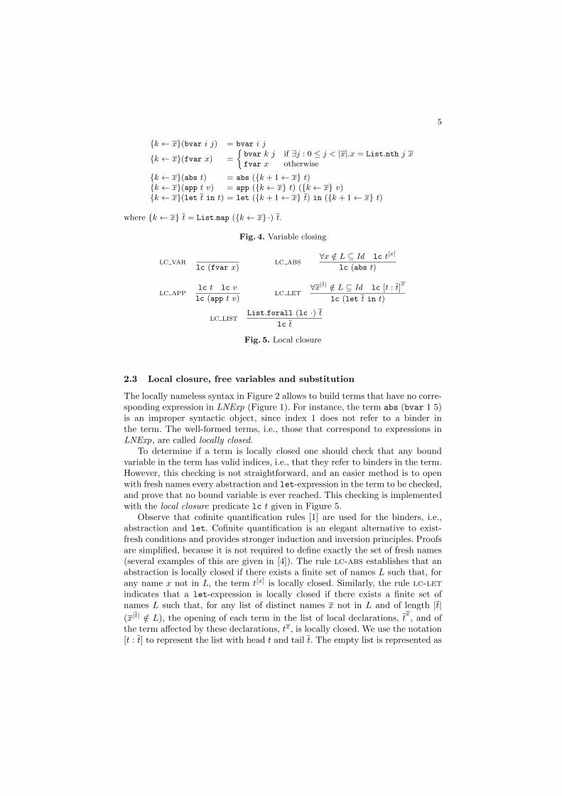
5
{k ← x}(bvar i j) = bvar i j
{k ← x}(fvar x) =
{bvar k j if ∃j : 0 ≤ j < |x|.x = List.nth j xfvar x otherwise
{k ← x}(abs t) = abs ({k + 1← x} t){k ← x}(app t v) = app ({k ← x} t) ({k ← x} v){k ← x}(let t in t) = let ({k + 1← x} t) in ({k + 1← x} t)
where {k ← x} t = List.map ({k ← x} ·) t.
Fig. 4. Variable closing
lc varlc (fvar x)
lc abs∀x /∈ L ⊆ Id lc t[x]
lc (abs t)
lc applc t lc v
lc (app t v)lc let
∀x|t| /∈ L ⊆ Id lc [t : t]x
lc (let t in t)
lc listList.forall (lc ·) t
lc t
Fig. 5. Local closure
2.3 Local closure, free variables and substitution
The locally nameless syntax in Figure 2 allows to build terms that have no corre-sponding expression in LNExp (Figure 1). For instance, the term abs (bvar 1 5)is an improper syntactic object, since index 1 does not refer to a binder inthe term. The well-formed terms, i.e., those that correspond to expressions inLNExp, are called locally closed.
To determine if a term is locally closed one should check that any boundvariable in the term has valid indices, i.e., that they refer to binders in the term.However, this checking is not straightforward, and an easier method is to openwith fresh names every abstraction and let-expression in the term to be checked,and prove that no bound variable is ever reached. This checking is implementedwith the local closure predicate lc t given in Figure 5.
Observe that cofinite quantification rules [1] are used for the binders, i.e.,abstraction and let. Cofinite quantification is an elegant alternative to exist-fresh conditions and provides stronger induction and inversion principles. Proofsare simplified, because it is not required to define exactly the set of fresh names(several examples of this are given in [4]). The rule lc-abs establishes that anabstraction is locally closed if there exists a finite set of names L such that, forany name x not in L, the term t[x] is locally closed. Similarly, the rule lc-letindicates that a let-expression is locally closed if there exists a finite set ofnames L such that, for any list of distinct names x not in L and of length |t|(x|t| /∈ L), the opening of each term in the list of local declarations, t
x, and of
the term affected by these declarations, tx, is locally closed. We use the notation[t : t] to represent the list with head t and tail t. The empty list is represented as

6
lck-bvari < k ∧ j < List.nth i n
lc at k n (bvar i j)lck-app
lc at k n t lc at k n v
lc at k n (app t v)
lck-fvarlc at k n (fvar x)
lck-letlc at (k + 1) [|t| : n] [t : t]
lc at k n (let t in t)
lck-abslc at (k + 1) [1 : n] t
lc at k n (abs t)lck-list
List.forall (lc at k n ·) tlc at k n t
Fig. 6. Closed at level k
[ ], a unitary list as [t], and [t : t] stands for t++[t], where ++ is the concatenationof lists.
Coming back to the first approach to local closure, i.e., checking that indicesin bound variables are valid, a new predicate is defined: t is closed at level k,written lc at k n t (Figure 6), where k indicates the current depth, that is, howmany binders have been passed by. As binders can be either abstractions or localdeclarations, we need to keep the size of each binder (1 in case of an abstraction,n for a let-expression with n local declarations). These sizes are collected in thelist n, thus |n| should be at least k. A bound variable bvar i j is closed at levelk if i is smaller than k and j is smaller than List.nth i n. The list n is newwith respect to [4] because there the predicate lc at is not defined for multiplebinders.
We can define an order between lists of natural numbers as follows:
[ ] ≥ [ ] m ≥ n ∧ m ≥ n⇒ [m : m] ≥ [n : n]
If a term t is locally closed at level k for a given list of numbers n, then it isalso locally closed at level k for any list of numbers greater than n.
Lemma 1.lc at m from n lc at k n t⇒ ∀m ≥ n . lc at k m t
The two approaches are equivalent, so that it can be proved that a term islocally closed if and only if it is closed at level 0.
Lemma 2.lc iif lc at lc t⇔ lc at 0 [ ] t
Computing the free variables of a term t is very easy in the locally namelessrepresentation, since bound and free variables are syntactically different. The setof free variables of t ∈ LNExp is denoted as fv(t), and it is defined in Figure 7.
A name x is said to be fresh for a term t, written fresh x in t, if x does notbelong to the set of free variables of t:
x /∈ fv(t)
fresh x in t

7
fv(bvar i j) = ∅ fv(fvar x) = {x}fv(app t v) = fv(t) ∪ fv(v) fv(abs t) = fv(t)fv(let t in t) = fv(t) ∪ fv(t)
where fv(t) = List.foldright (· ∪ ·) ∅ (List.map fv t).
Fig. 7. Free variables
(bvar i j)[z/y] = bvar i j (fvar x)[z/y] =
{fvar z if x = yfvar x if x 6= y
(abs t)[z/y] = abs t[z/y] (app t v)[z/y] = app t[z/y] v[z/y](let t in t)[z/y] = let t[z/y] in t[z/y]
where t[z/y] = List.map ([z/y]·) t.
Fig. 8. Substitution
This definition can be easily extended to a list of distinct names x:
x /∈ fv(t)
fresh x in t
A term t is closed if it has no free variables at all:
fv(t) = ∅closed t
Substitution replaces a variable name by another name in a term. So that fort ∈ LNExp and z, y ∈ Id , t[z/y] is the term where z substitutes any occurrenceof y in t (see Figure 8).
Under some conditions variable closing and variable opening are inverse op-erations. More precisely, opening a term with fresh names and closing it with thesame names, produces the original term. Symmetrically, closing a locally closedterm t and then opening it with the same names gives back t.
Lemma 3.close open var fresh x in t⇒ \x(tx) = topen close var lc t⇒ (\xt)x = t
3 Natural semantics for lazy λ-calculus
The natural semantics defined by Launchbury [6] follows a lazy strategy. Judge-ments are of the form Γ : e ⇓ ∆ : w, that is, the expression e ∈ Exp in thecontext of the heap Γ reduces to the value w in the context of the (modified)heap ∆. Values (w ∈ Val) are expressions in weak-head-normal-form (whnf ).Heaps are partial functions from variables into expressions. Each pair (variable,expression) is called a binding, and it is represented by x 7→ e. During evaluation,new bindings may be added to the heap, and bindings may be updated to their
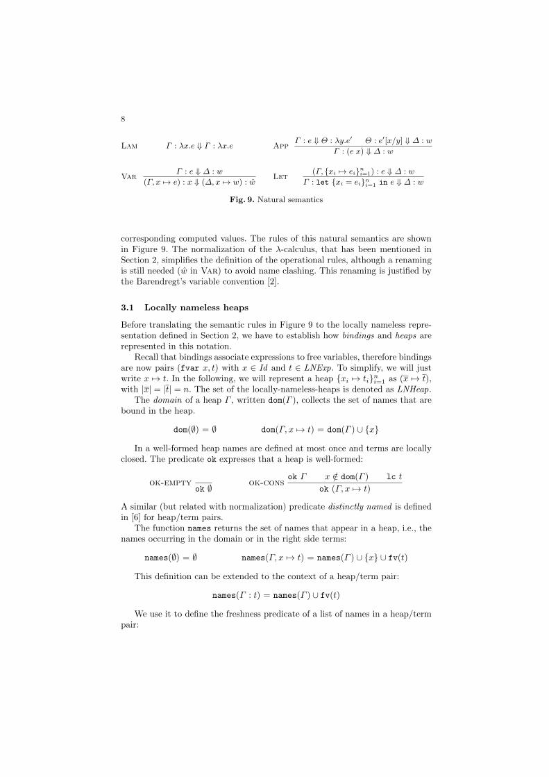
8
Lam Γ : λx.e ⇓ Γ : λx.e AppΓ : e ⇓ Θ : λy.e′ Θ : e′[x/y] ⇓ ∆ : w
Γ : (e x) ⇓ ∆ : w
VarΓ : e ⇓ ∆ : w
(Γ, x 7→ e) : x ⇓ (∆,x 7→ w) : wLet
(Γ, {xi 7→ ei}ni=1) : e ⇓ ∆ : w
Γ : let {xi = ei}ni=1 in e ⇓ ∆ : w
Fig. 9. Natural semantics
corresponding computed values. The rules of this natural semantics are shownin Figure 9. The normalization of the λ-calculus, that has been mentioned inSection 2, simplifies the definition of the operational rules, although a renamingis still needed (w in Var) to avoid name clashing. This renaming is justified bythe Barendregt’s variable convention [2].
3.1 Locally nameless heaps
Before translating the semantic rules in Figure 9 to the locally nameless repre-sentation defined in Section 2, we have to establish how bindings and heaps arerepresented in this notation.
Recall that bindings associate expressions to free variables, therefore bindingsare now pairs (fvar x, t) with x ∈ Id and t ∈ LNExp. To simplify, we will justwrite x 7→ t. In the following, we will represent a heap {xi 7→ ti}ni=1 as (x 7→ t),with |x| = |t| = n. The set of the locally-nameless-heaps is denoted as LNHeap.
The domain of a heap Γ , written dom(Γ ), collects the set of names that arebound in the heap.
dom(∅) = ∅ dom(Γ, x 7→ t) = dom(Γ ) ∪ {x}
In a well-formed heap names are defined at most once and terms are locallyclosed. The predicate ok expresses that a heap is well-formed:
ok-emptyok ∅ ok-cons
ok Γ x /∈ dom(Γ ) lc t
ok (Γ, x 7→ t)
A similar (but related with normalization) predicate distinctly named is definedin [6] for heap/term pairs.
The function names returns the set of names that appear in a heap, i.e., thenames occurring in the domain or in the right side terms:
names(∅) = ∅ names(Γ, x 7→ t) = names(Γ ) ∪ {x} ∪ fv(t)
This definition can be extended to the context of a heap/term pair:
names(Γ : t) = names(Γ ) ∪ fv(t)
We use it to define the freshness predicate of a list of names in a heap/termpair:
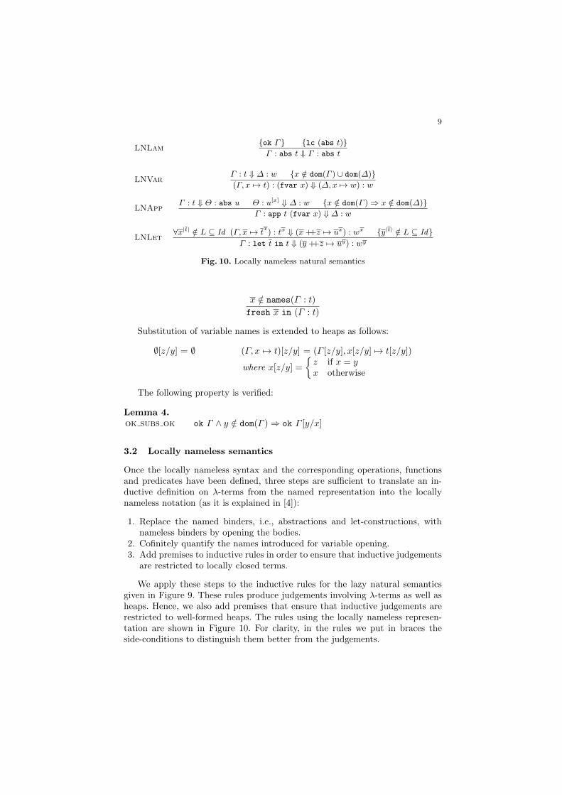
9
LNLam{ok Γ} {lc (abs t)}Γ : abs t ⇓ Γ : abs t
LNVarΓ : t ⇓ ∆ : w {x /∈ dom(Γ ) ∪ dom(∆)}(Γ, x 7→ t) : (fvar x) ⇓ (∆,x 7→ w) : w
LNAppΓ : t ⇓ Θ : abs u Θ : u[x] ⇓ ∆ : w {x /∈ dom(Γ )⇒ x /∈ dom(∆)}
Γ : app t (fvar x) ⇓ ∆ : w
LNLet∀x|t| /∈ L ⊆ Id (Γ, x 7→ t
x) : tx ⇓ (x++z 7→ ux) : wx {y|t| /∈ L ⊆ Id}
Γ : let t in t ⇓ (y ++z 7→ uy) : wy
Fig. 10. Locally nameless natural semantics
x /∈ names(Γ : t)
fresh x in (Γ : t)
Substitution of variable names is extended to heaps as follows:
∅[z/y] = ∅ (Γ, x 7→ t)[z/y] = (Γ [z/y], x[z/y] 7→ t[z/y])
where x[z/y] =
{z if x = yx otherwise
The following property is verified:
Lemma 4.ok subs ok ok Γ ∧ y /∈ dom(Γ )⇒ ok Γ [y/x]
3.2 Locally nameless semantics
Once the locally nameless syntax and the corresponding operations, functionsand predicates have been defined, three steps are sufficient to translate an in-ductive definition on λ-terms from the named representation into the locallynameless notation (as it is explained in [4]):
1. Replace the named binders, i.e., abstractions and let-constructions, withnameless binders by opening the bodies.
2. Cofinitely quantify the names introduced for variable opening.3. Add premises to inductive rules in order to ensure that inductive judgements
are restricted to locally closed terms.
We apply these steps to the inductive rules for the lazy natural semanticsgiven in Figure 9. These rules produce judgements involving λ-terms as well asheaps. Hence, we also add premises that ensure that inductive judgements arerestricted to well-formed heaps. The rules using the locally nameless represen-tation are shown in Figure 10. For clarity, in the rules we put in braces theside-conditions to distinguish them better from the judgements.

10
The main difference with the rules in Figure 9 is the rule LNLet. To evaluatelet t in t the local terms t have to be introduced in the heap, so that the bodyt is evaluated in this new context. To this purpose fresh names x are needed toopen the local terms and the body. The evaluation of tx produces a final heapand a value. Both are dependent on the names chosen for the local variables. Thedomain of the final heap consists of the local names x and the rest of names, sayz. The rule LNLet is cofinite quantified. As it is explained in [4], the advantageof the cofinite rules over existential and universal ones is that the freshness side-conditions are not explicit. The freshness condition for x is hidden in the finiteset L, which includes the names that should be avoided during the reduction.The novelty of our cofinite rule, compared with the ones appearing in [1] and [4](that are similar to the cofinite rules for the predicate lc in Figure 5), is thatthe names introduced in the (infinite) premises do appear in the conclusion too.Therefore, in the conclusion of the rule LNLet we can replace the names x byany list y not in L.
The problem with explicit freshness conditions is that they are associatedjust to rule instances, while they should apply to the whole reduction proof.Take for instance the rule LNVar. In the premise the binding x 7→ t does nolonger belong to the heap. Therefore, a valid reduction for this premise maychose x as fresh. We avoid this situation by requiring that x is undefined in thefinal heap too.6 By contrast to the rule Var in Figure 9, no renaming of thefinal value, that is w, is needed.
The side-condition of rule LNApp deserves an explanation too. Let us sup-pose that x is undefined in the initial heap Γ . We must avoid that x is chosenas a fresh name during the evaluation of t. For this reason we require that x isdefined in the final heap ∆ only if x was already defined in Γ . Notice how thebody of the abstraction, that is u, is open with the name x. This is equivalentto the substitution of x for y in the body of the abstraction λy.e′ (see rule Appin Figure 9).
A regularity lemma ensures that the judgements produced by this reductionsystem involve only well-formed heaps and locally closed terms.
Lemma 5.regularity Γ : t ⇓ ∆ : w ⇒ ok Γ ∧ lc t ∧ ok ∆ ∧ lc w.
Similarly, Theorem 1 in [6] ensures that the property of being distinctly namedis preserved by the rules in Figure 9.
The next lemma states that names defined in a context heap remain definedafter the evaluation of any term in that context.
Lemma 6.def not lost Γ : t ⇓ ∆ : w ⇒ dom(Γ ) ⊆ dom(∆).
6 An alternative is to decorate judgements with a set collecting the names that havebeen taken out of the heap during a reduction proof, and starting with the emptyset. This approach has been adopted by Sestoft in [7].

11
Moreover, fresh names are only introduced by the rule LNLet and, conse-quently, they are bound in the final heap/value pair. Therefore, any undefinedfree variable appearing in the final heap/value pair must occur in the initialheap/term pair too.
Lemma 7.add vars Γ : t ⇓ ∆ : w
⇒ (x ∈ names(∆ : w)⇒ (x ∈ dom(∆) ∨ x ∈ names(Γ : t))).
A renaming lemma ensures that the evaluation of a term is independent ofthe fresh names chosen in the reduction process. Moreover, any name in thecontext can be replaced by a fresh one without changing the meaning of theterms evaluated in that context. In fact, reduction proofs for heap/term pairsare unique up to α-conversion of the names defined in the context heap.
Lemma 8.renaming Γ : t ⇓ ∆ : w ∧ fresh y in (Γ : t) ∧ fresh y in (∆ : w)
⇒ Γ [y/x] : t[y/x] ⇓ ∆[y/x] : w[y/x].
In addition, the renaming lemma permits to prove an introduction lemmafor the cofinite rule LNLet which establishes that the corresponding existentialrule is admissible too.
Lemma 9.let intro (Γ, x 7→ t
x) : tx ⇓ (x++z 7→ ux) : wx ∧ fresh x in (Γ : let t in t)
⇒ Γ : let t in t ⇓ (x++z 7→ ux) : wx.
This result, together with the renaming lemma, justifies that our rule LNLetis equivalent to Launchbury’s rule Let used with normalized terms.
4 Conclusions and future work
In the present work we have used a locally nameless representation not only forthe pure λ-calculus [4] but also for its extension with mutually recursive localdeclarations. This notation avoids name clashing between bound and free vari-ables. Afterwards, we have used this representation for redefining Launchbury’snatural semantics for lazy evaluation [6]. To this purpose we have adapted thedefinition of context heaps to the locally nameless notation. A heap may be seenas a multiple binder. Actually, the names defined (bound) in a heap can be re-placed by other names, provided that terms keep their meaning in the contextrepresented by the heap. Our renaming lemma ensures that whenever a heap isrenamed with fresh names, reduction proofs are preserved.
Launchbury assumes Barendregt’s variable convention [2] in [6] when defininghis operational semantics only for normalized λ-terms. In order to the avoid thisproblematic [8] variable convention, we have used cofinite quantification in ourlocally nameless reduction rules. Freshness conditions are usually considered ineach rule individually. Nevertheless, this technique produces name clashing when
12
considering whole reduction proofs. A solution might be to decorate each rulewith the set of forbidden names and indicate how to modify this set duringthe reduction process. However, this could be too restrictive in many occasions.Moreover, existential rules are not easy to deal with because each reduction isobtained just for one specific list of names. If any of the names in this list causes aname clashing with other reduction proofs, then it is cumbersome to demonstratethat an alternative reduction for a fresh list does exist. Cofinite quantificationhas allowed us to solve this problem because in a single step reductions areguaranteed for an infinite number of lists of names. Moreover, our introductionlemma guarantees that a more conventional exists-fresh rule is correct in ourreduction system too.
The cofinite quantification that we have used in our semantic rules is morecomplex than those in [1] and [4]. Our cofinite rule LNLet in Figure 10 intro-duces quantified variables in the conclusion as well, as the latter depends on thechosen names.
Our future tasks include the implementation in the proof assistant Coq [3]of the natural semantics redefined in this paper. The final aim is to prove auto-matically the equivalence of the natural semantics with the alternative versiongiven also in [6]. This alternative version differs from the original one in the in-troduction of indirections during β-reduction and the elimination of updates. Atpresent we are working on the definition (using the locally nameless representa-tion) of two intermediate semantics, one introducing indirections and the otherwithout updates. Then, we will establish equivalence relations between heapsobtained by each semantics, which allow us to prove the equivalence of the orig-inal natural semantics and the alternative semantics through the intermediatesemantics.
5 Acknowledgments
This work is partially supported by the projects: TIN2009-14599-C03-01 andS2009/TIC-1465.
References
1. B. E. Aydemir, A. Chargueraud, B. C. Pierce, R. Pollack, and S. Weirich. En-gineering formal metatheory. In ACM Symposium on Principles of ProgrammingLanguages, POPL’08, pages 3–15. ACM Press, 2008.
2. H. P. Barendregt. The Lambda Calculus: Its Syntax and Semantics, volume 103 ofStudies in Logic and the Foundations of Mathematics. North-Holland, 1984.
3. Y. Bertot. Coq in a hurry. CoRR, abs/cs/0603118, 2006.4. A. Chargueraud. The locally nameless representation. Journal of Automated Rea-
soning, pages 1–46, 2011.5. N. G. de Bruijn. Lambda calculus notation with nameless dummies, a tool for
automatic formula manipulation, with application to the Church-Rosser theorem.Indagationes Mathematicae, 75(5):381–392, 1972.
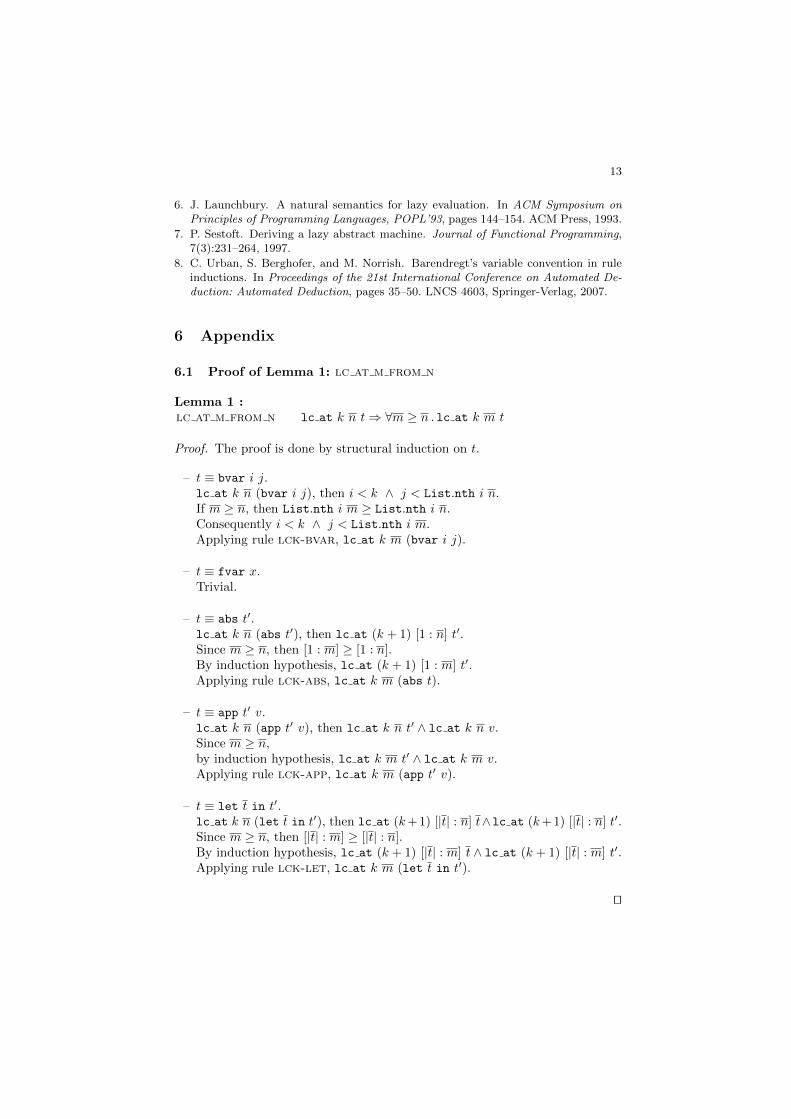
13
6. J. Launchbury. A natural semantics for lazy evaluation. In ACM Symposium onPrinciples of Programming Languages, POPL’93, pages 144–154. ACM Press, 1993.
7. P. Sestoft. Deriving a lazy abstract machine. Journal of Functional Programming,7(3):231–264, 1997.
8. C. Urban, S. Berghofer, and M. Norrish. Barendregt’s variable convention in ruleinductions. In Proceedings of the 21st International Conference on Automated De-duction: Automated Deduction, pages 35–50. LNCS 4603, Springer-Verlag, 2007.
6 Appendix
6.1 Proof of Lemma 1: lc at m from n
Lemma 1 :lc at m from n lc at k n t⇒ ∀m ≥ n . lc at k m t
Proof. The proof is done by structural induction on t.
– t ≡ bvar i j.lc at k n (bvar i j), then i < k ∧ j < List.nth i n.If m ≥ n, then List.nth i m ≥ List.nth i n.Consequently i < k ∧ j < List.nth i m.Applying rule lck-bvar, lc at k m (bvar i j).
– t ≡ fvar x.Trivial.
– t ≡ abs t′.lc at k n (abs t′), then lc at (k + 1) [1 : n] t′.Since m ≥ n, then [1 : m] ≥ [1 : n].By induction hypothesis, lc at (k + 1) [1 : m] t′.Applying rule lck-abs, lc at k m (abs t).
– t ≡ app t′ v.lc at k n (app t′ v), then lc at k n t′ ∧ lc at k n v.Since m ≥ n,by induction hypothesis, lc at k m t′ ∧ lc at k m v.Applying rule lck-app, lc at k m (app t′ v).
– t ≡ let t in t′.lc at k n (let t in t′), then lc at (k+1) [|t| : n] t∧lc at (k+1) [|t| : n] t′.Since m ≥ n, then [|t| : m] ≥ [|t| : n].By induction hypothesis, lc at (k + 1) [|t| : m] t ∧ lc at (k + 1) [|t| : m] t′.Applying rule lck-let, lc at k m (let t in t′).
ut

14
6.2 Proof of Lemma 2: lc iif lc at
To prove Lemma 2, we have to prove two auxiliary results: Lemmas 10 and 11.If a term t opened with names x at level k is locally closed at level k with n,
then the term t is also locally closed at level k + 1 with [n : |x|].Lemma 10.lc at k+1 from k k= |n| ∧ lc at k n ({k→x}t)⇒ lc at (k + 1) [n : |x|] tProof. The proof is done by induction on the structure of t.
– t ≡ bvar i j.lc at k n ({k → x}(bvar i j)).• i = k ∧ j < |x|
By hypothesis, lc at k n (fvar (List.nth j x))Thus,
i = k < k + 1 ∧ j < |x| k=|n|= List.nth k [n : |x|] = List.nth i [n : |x|].
• otherwiseBy hypothesis, lc at k n (bvar i j), then i < k ∧ j < List.nth i n.Thus, i < k < k + 1 ∧ j < List.nth i n = List.nth i [n : |x|].
In both cases, by rule lck-bvar, lc at (k + 1) [n : |x|] (bvar i j).
– t ≡ fvar x.Trivial.
– t ≡ abs t′.Since lc at k n ({k → x}(abs t′)), lc at k n (abs ({k + 1→ x}t′)).Thus, lc at (k + 1) [1 : n] ({k + 1→ x}t′).By induction hypothesis, lc at (k + 2) [1 : n : |x|] t′.Applying rule lck-abs, lc at (k + 1) [n : |x|] (abs t′).
– t ≡ app t′ v.Since lc at k n ({k → x}(app t′ v)),lc at k n (app ({k → x}t′) ({k → x}v)).Thus, lc at k n ({k → x}t′) ∧ lc at k n ({k → x}v).By induction hypothesis, lc at (k + 1) [n : |x|] t′ ∧ lc at (k + 1) [n : |x|] v.Applying rule lck-app, lc at (k + 1) [n : |x|] (app t′ v).
– t ≡ let t in t′.Since lc at k n ({k → x}(let t in t′)),lc at k n (let ({k + 1→ x}t) in ({k + 1→ x}t′)).Thus, lc at (k + 1) [|t| : n] ({k + 1→ x}t)and lc at (k + 1) [|t| : n] ({k + 1→ x}t′).By induction hypothesis,lc at (k + 2) [|t| : n : |x|] t ∧ lc at (k + 2) [|t| : n : |x|] t′.Applying rule lck-let, lc at (k + 1) [n : |x|] (let t in t′).
ut
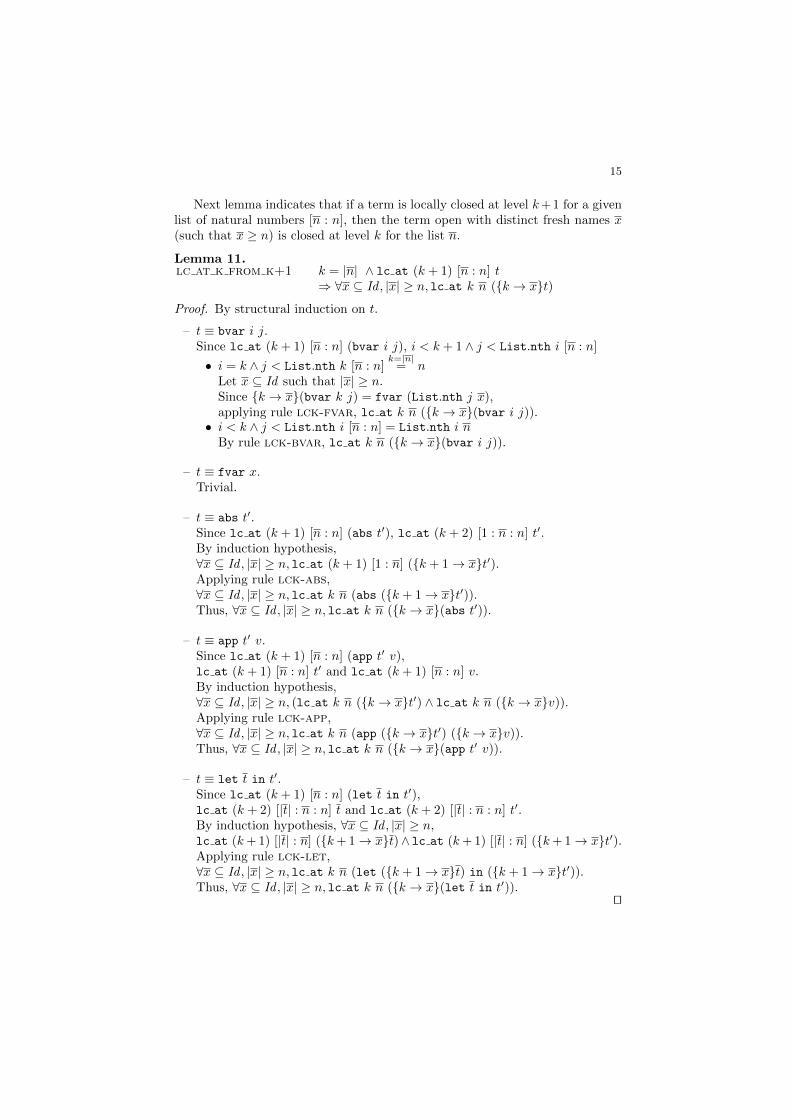
15
Next lemma indicates that if a term is locally closed at level k+1 for a givenlist of natural numbers [n : n], then the term open with distinct fresh names x(such that x ≥ n) is closed at level k for the list n.
Lemma 11.lc at k from k+1 k = |n| ∧ lc at (k + 1) [n : n] t
⇒ ∀x ⊆ Id , |x| ≥ n, lc at k n ({k → x}t)Proof. By structural induction on t.
– t ≡ bvar i j.Since lc at (k + 1) [n : n] (bvar i j), i < k + 1 ∧ j < List.nth i [n : n]
• i = k ∧ j < List.nth k [n : n]k=|n|
= nLet x ⊆ Id such that |x| ≥ n.Since {k → x}(bvar k j) = fvar (List.nth j x),applying rule lck-fvar, lc at k n ({k → x}(bvar i j)).
• i < k ∧ j < List.nth i [n : n] = List.nth i nBy rule lck-bvar, lc at k n ({k → x}(bvar i j)).
– t ≡ fvar x.Trivial.
– t ≡ abs t′.Since lc at (k + 1) [n : n] (abs t′), lc at (k + 2) [1 : n : n] t′.By induction hypothesis,∀x ⊆ Id , |x| ≥ n, lc at (k + 1) [1 : n] ({k + 1→ x}t′).Applying rule lck-abs,∀x ⊆ Id , |x| ≥ n, lc at k n (abs ({k + 1→ x}t′)).Thus, ∀x ⊆ Id , |x| ≥ n, lc at k n ({k → x}(abs t′)).
– t ≡ app t′ v.Since lc at (k + 1) [n : n] (app t′ v),lc at (k + 1) [n : n] t′ and lc at (k + 1) [n : n] v.By induction hypothesis,∀x ⊆ Id , |x| ≥ n, (lc at k n ({k → x}t′) ∧ lc at k n ({k → x}v)).Applying rule lck-app,∀x ⊆ Id , |x| ≥ n, lc at k n (app ({k → x}t′) ({k → x}v)).Thus, ∀x ⊆ Id , |x| ≥ n, lc at k n ({k → x}(app t′ v)).
– t ≡ let t in t′.Since lc at (k + 1) [n : n] (let t in t′),lc at (k + 2) [|t| : n : n] t and lc at (k + 2) [|t| : n : n] t′.By induction hypothesis, ∀x ⊆ Id , |x| ≥ n,lc at (k+ 1) [|t| : n] ({k+ 1→ x}t)∧ lc at (k+ 1) [|t| : n] ({k+ 1→ x}t′).Applying rule lck-let,∀x ⊆ Id , |x| ≥ n, lc at k n (let ({k + 1→ x}t) in ({k + 1→ x}t′)).Thus, ∀x ⊆ Id , |x| ≥ n, lc at k n ({k → x}(let t in t′)).
ut
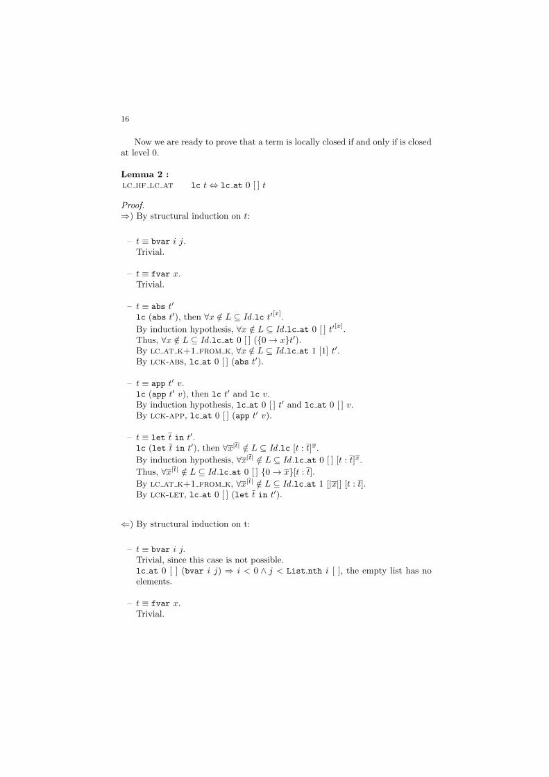
16
Now we are ready to prove that a term is locally closed if and only if is closedat level 0.
Lemma 2 :lc iif lc at lc t⇔ lc at 0 [ ] t
Proof.⇒) By structural induction on t:
– t ≡ bvar i j.Trivial.
– t ≡ fvar x.Trivial.
– t ≡ abs t′
lc (abs t′), then ∀x /∈ L ⊆ Id .lc t′[x].
By induction hypothesis, ∀x /∈ L ⊆ Id .lc at 0 [ ] t′[x].Thus, ∀x /∈ L ⊆ Id .lc at 0 [ ] ({0→ x}t′).By lc at k+1 from k, ∀x /∈ L ⊆ Id .lc at 1 [1] t′.By lck-abs, lc at 0 [ ] (abs t′).
– t ≡ app t′ v.lc (app t′ v), then lc t′ and lc v.By induction hypothesis, lc at 0 [ ] t′ and lc at 0 [ ] v.By lck-app, lc at 0 [ ] (app t′ v).
– t ≡ let t in t′.lc (let t in t′), then ∀x|t| /∈ L ⊆ Id .lc [t : t]x.
By induction hypothesis, ∀x|t| /∈ L ⊆ Id .lc at 0 [ ] [t : t]x.
Thus, ∀x|t| /∈ L ⊆ Id .lc at 0 [ ] {0→ x}[t : t].
By lc at k+1 from k, ∀x|t| /∈ L ⊆ Id .lc at 1 [|x|] [t : t].By lck-let, lc at 0 [ ] (let t in t′).
⇐) By structural induction on t:
– t ≡ bvar i j.Trivial, since this case is not possible.lc at 0 [ ] (bvar i j) ⇒ i < 0 ∧ j < List.nth i [ ], the empty list has noelements.
– t ≡ fvar x.Trivial.
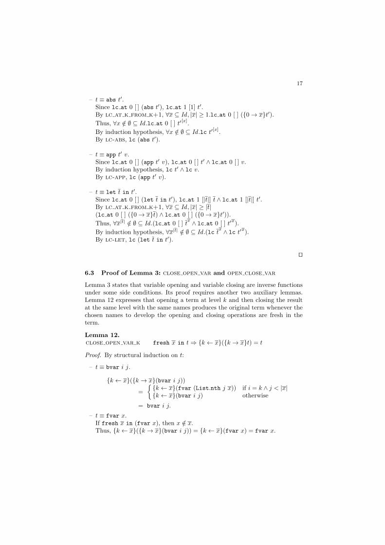
17
– t ≡ abs t′.Since lc at 0 [ ] (abs t′), lc at 1 [1] t′.By lc at k from k+1, ∀x ⊆ Id , |x| ≥ 1.lc at 0 [ ] ({0→ x}t′).Thus, ∀x /∈ ∅ ⊆ Id .lc at 0 [ ] t′[x].
By induction hypothesis, ∀x /∈ ∅ ⊆ Id .lc t′[x].By lc-abs, lc (abs t′).
– t ≡ app t′ v.Since lc at 0 [ ] (app t′ v), lc at 0 [ ] t′ ∧ lc at 0 [ ] v.By induction hypothesis, lc t′ ∧ lc v.By lc-app, lc (app t′ v).
– t ≡ let t in t′.Since lc at 0 [ ] (let t in t′), lc at 1 [|t|] t ∧ lc at 1 [|t|] t′.By lc at k from k+1, ∀x ⊆ Id , |x| ≥ |t|(lc at 0 [ ] ({0→ x}t) ∧ lc at 0 [ ] ({0→ x}t′)).Thus, ∀x|t| /∈ ∅ ⊆ Id .(lc at 0 [ ] t
x ∧ lc at 0 [ ] t′x).
By induction hypothesis, ∀x|t| /∈ ∅ ⊆ Id .(lc tx ∧ lc t′x).
By lc-let, lc (let t in t′).
ut
6.3 Proof of Lemma 3: close open var and open close var
Lemma 3 states that variable opening and variable closing are inverse functionsunder some side conditions. Its proof requires another two auxiliary lemmas.Lemma 12 expresses that opening a term at level k and then closing the resultat the same level with the same names produces the original term whenever thechosen names to develop the opening and closing operations are fresh in theterm.
Lemma 12.close open var k fresh x in t⇒ {k ← x}({k → x}t) = t
Proof. By structural induction on t:
– t ≡ bvar i j.
{k ← x}({k → x}(bvar i j))=
{{k ← x}(fvar (List.nth j x)) if i = k ∧ j < |x|{k ← x}(bvar i j) otherwise
= bvar i j.
– t ≡ fvar x.If fresh x in (fvar x), then x /∈ x.Thus, {k ← x}({k → x}(bvar i j)) = {k ← x}(fvar x) = fvar x.
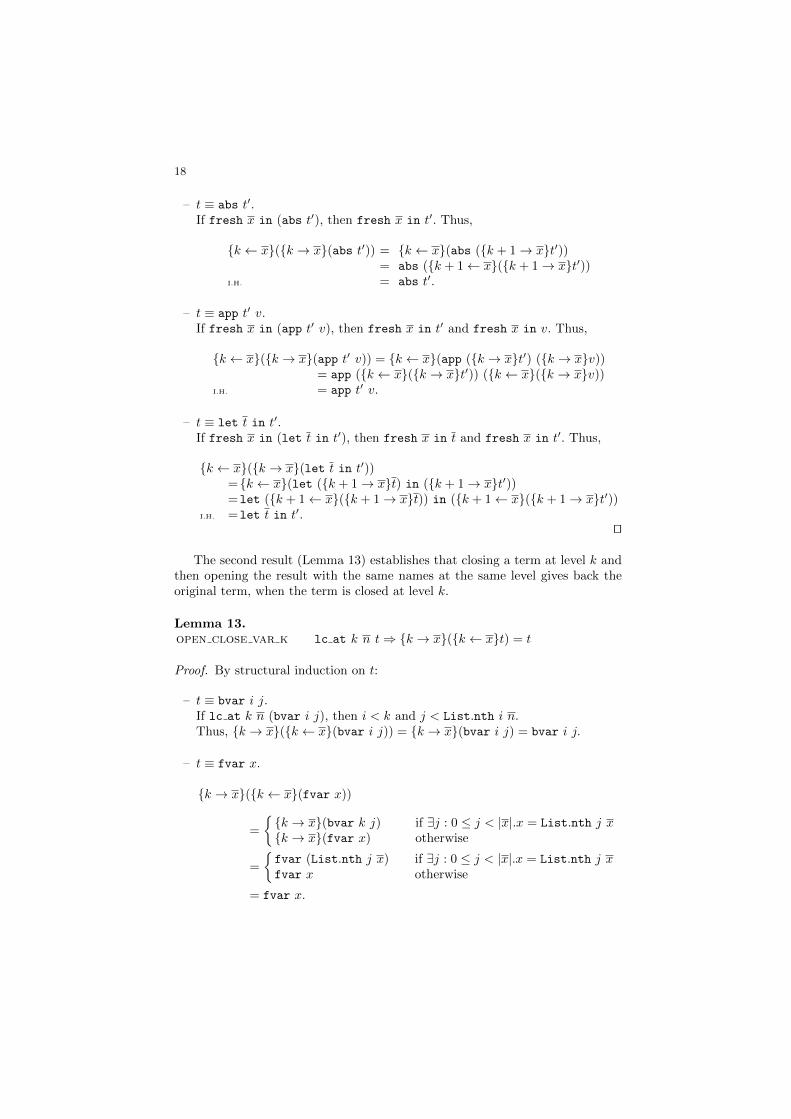
18
– t ≡ abs t′.If fresh x in (abs t′), then fresh x in t′. Thus,
{k ← x}({k → x}(abs t′)) = {k ← x}(abs ({k + 1→ x}t′))= abs ({k + 1← x}({k + 1→ x}t′))
I.H. = abs t′.
– t ≡ app t′ v.If fresh x in (app t′ v), then fresh x in t′ and fresh x in v. Thus,
{k ← x}({k → x}(app t′ v)) = {k ← x}(app ({k → x}t′) ({k → x}v))= app ({k ← x}({k → x}t′)) ({k ← x}({k → x}v))
I.H. = app t′ v.
– t ≡ let t in t′.If fresh x in (let t in t′), then fresh x in t and fresh x in t′. Thus,
{k ← x}({k → x}(let t in t′))={k ← x}(let ({k + 1→ x}t) in ({k + 1→ x}t′))=let ({k + 1← x}({k + 1→ x}t)) in ({k + 1← x}({k + 1→ x}t′))
I.H. =let t in t′.ut
The second result (Lemma 13) establishes that closing a term at level k andthen opening the result with the same names at the same level gives back theoriginal term, when the term is closed at level k.
Lemma 13.open close var k lc at k n t⇒ {k → x}({k ← x}t) = t
Proof. By structural induction on t:
– t ≡ bvar i j.If lc at k n (bvar i j), then i < k and j < List.nth i n.Thus, {k → x}({k ← x}(bvar i j)) = {k → x}(bvar i j) = bvar i j.
– t ≡ fvar x.
{k → x}({k ← x}(fvar x))
=
{{k → x}(bvar k j) if ∃j : 0 ≤ j < |x|.x = List.nth j x{k → x}(fvar x) otherwise
=
{fvar (List.nth j x) if ∃j : 0 ≤ j < |x|.x = List.nth j xfvar x otherwise
= fvar x.

19
– t ≡ abs t′.If lc at k n (abs t′), then lc at (k + 1) [1 : n] t′. Thus,
{k → x}({k ← x}(abs t′)) = {k → x}(abs ({k + 1← x}t′))= abs ({k + 1→ x}({k + 1← x}t′))
I.H. = abs t′
– t ≡ app t′ v.If lc at k n (app t′ v), then lc at k n t′ and lc at k n v. Thus,
{k → x}({k ← x}(app t′ v)) = {k → x}(app ({k ← x}t′) ({k ← x}v))= app ({k → x}({k ← x}t′)) ({k → x}({k ← x}v))
I.H. = app t′ v
– t ≡ let t in t′.If lc at k n (let t in t′), thenlc at (k + 1) [|t| : n] t and lc at (k + 1) [|t| : n] t′. Thus,
{k → x}({k ← x}(let t in t′))= {k → x}(let ({k + 1← x}t) in ({k + 1← x}t′))= let ({k + 1→ x}({k + 1← x}t)) in ({k + 1→ x}({k + 1← x}t′))
I.H. = let t in t′.ut
Now the proof of Lemma 3 is straightforward.
Lemma 3close open var fresh x in t⇒ \x(tx) = topen close var lc t⇒ (\xt)x = t
Proof.
– close open var is a corollary of Lemma 12 (take k = 0).– open close var is a corollary of Lemma 13 (take k = 0).
ut
6.4 Proof of Lemma 4: ok subs ok
Lemmas 14 and 15 are needed to prove Lemma 4. Every variable in the domainof a heap where variable x has been substituted by y is either in the domain ofthe original heap, or coincides with y.
Lemma 14.dom subs union dom(Γ [y/x]) ⊆ dom(Γ ) ∪ {y}
Proof. By induction on the size of Γ :
– Γ = ∅. Trivial.
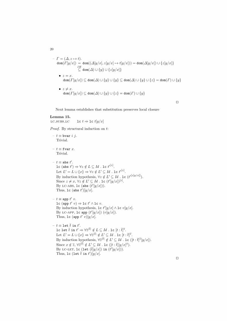
20
– Γ = (∆, z 7→ t).dom(Γ [y/x]) = dom((∆[y/x], z[y/x] 7→ t[y/x])) = dom(∆[y/x]) ∪ {z[y/x]}
IH⊆ dom(∆) ∪ {y} ∪ {z[y/x]}
• z = x.dom(Γ [y/x]) ⊆ dom(∆) ∪ {y} ∪ {y} ⊆ dom(∆) ∪ {y} ∪ {z} = dom(Γ ) ∪ {y}
• z 6= x.dom(Γ [y/x]) ⊆ dom(∆) ∪ {y} ∪ {z} = dom(Γ ) ∪ {y}
ut
Next lemma establishes that substitution preserves local closure
Lemma 15.lc subs lc lc t⇒ lc t[y/x]
Proof. By structural induction on t:
– t ≡ bvar i j.Trivial.
– t ≡ fvar x.Trivial.
– t ≡ abs t′.lc (abs t′)⇒ ∀z /∈ L ⊆ Id . lc t′[z].
Let L′ = L ∪ {x} ⇒ ∀z /∈ L′ ⊆ Id . lc t′[z].
By induction hypothesis, ∀z /∈ L′ ⊆ Id . lc (t′[z[y/x]]).Since z 6= x, ∀z /∈ L′ ⊆ Id . lc (t′[y/x])[z].By lc-abs, lc (abs (t′[y/x])).Thus, lc (abs t′)[y/x].
– t ≡ app t′ v.lc (app t′ v)⇒ lc t′ ∧ lc v.By induction hypothesis, lc t′[y/x] ∧ lc v[y/x].By lc-app, lc app (t′[y/x]) (v[y/x]).Thus, lc (app t′ v)[y/x].
– t ≡ let t in t′.lc let t in t′ ⇒ ∀z|t| /∈ L ⊆ Id . lc [t : t]z.
Let L′ = L ∪ {x} ⇒ ∀z|t| /∈ L′ ⊆ Id . lc [t : t]z.
By induction hypothesis, ∀z|t| /∈ L′ ⊆ Id . lc ([t : t]z[y/x]).
Since x /∈ z, ∀z|t| /∈ L′ ⊆ Id . lc ([t : t][y/x]z).By lc-let, lc (let (t[y/x]) in (t′[y/x])).Thus, lc (let t in t′)[y/x].
ut
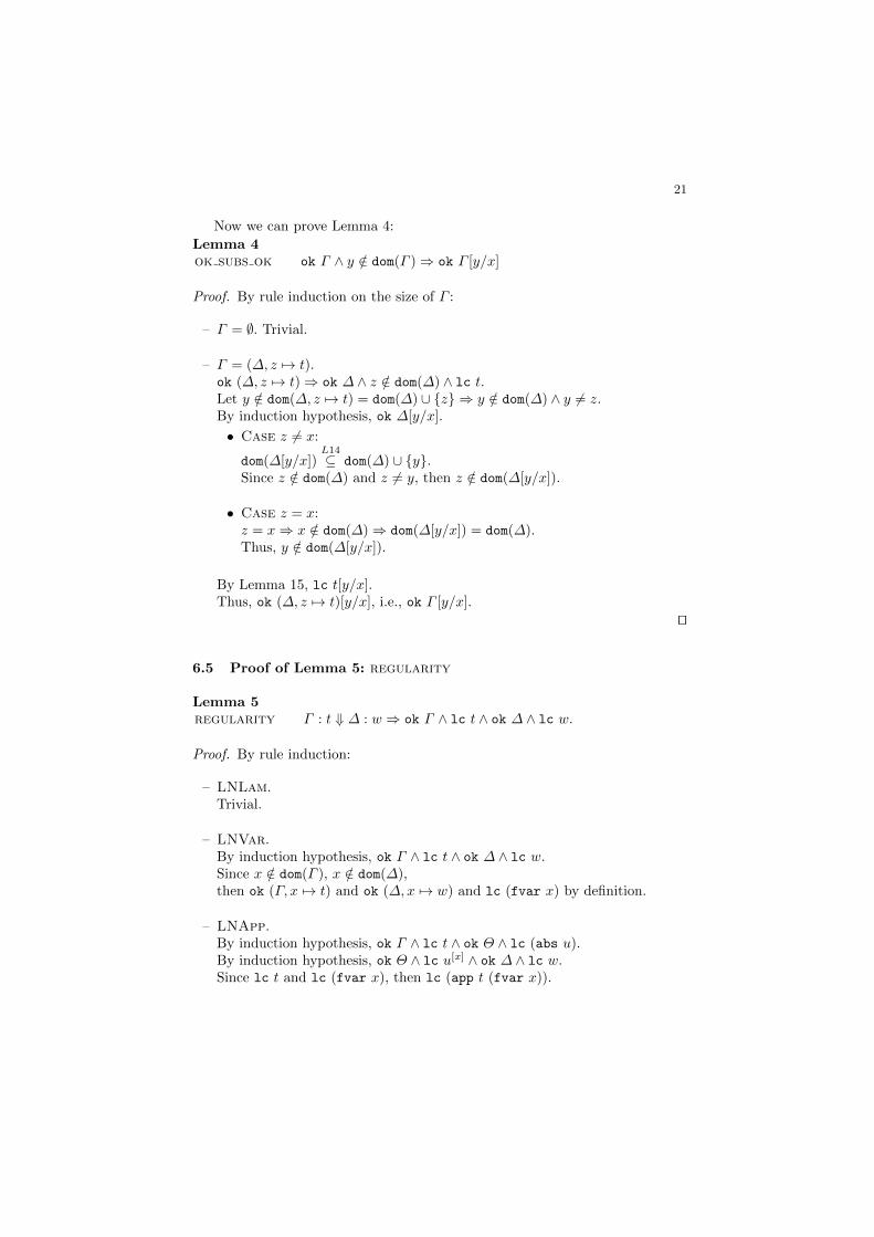
21
Now we can prove Lemma 4:
Lemma 4ok subs ok ok Γ ∧ y /∈ dom(Γ )⇒ ok Γ [y/x]
Proof. By rule induction on the size of Γ :
– Γ = ∅. Trivial.
– Γ = (∆, z 7→ t).ok (∆, z 7→ t)⇒ ok ∆ ∧ z /∈ dom(∆) ∧ lc t.Let y /∈ dom(∆, z 7→ t) = dom(∆) ∪ {z} ⇒ y /∈ dom(∆) ∧ y 6= z.By induction hypothesis, ok ∆[y/x].
• Case z 6= x:
dom(∆[y/x])L14⊆ dom(∆) ∪ {y}.
Since z /∈ dom(∆) and z 6= y, then z /∈ dom(∆[y/x]).
• Case z = x:z = x⇒ x /∈ dom(∆)⇒ dom(∆[y/x]) = dom(∆).Thus, y /∈ dom(∆[y/x]).
By Lemma 15, lc t[y/x].Thus, ok (∆, z 7→ t)[y/x], i.e., ok Γ [y/x].
ut
6.5 Proof of Lemma 5: regularity
Lemma 5regularity Γ : t ⇓ ∆ : w ⇒ ok Γ ∧ lc t ∧ ok ∆ ∧ lc w.
Proof. By rule induction:
– LNLam.Trivial.
– LNVar.By induction hypothesis, ok Γ ∧ lc t ∧ ok ∆ ∧ lc w.Since x /∈ dom(Γ ), x /∈ dom(∆),then ok (Γ, x 7→ t) and ok (∆,x 7→ w) and lc (fvar x) by definition.
– LNApp.By induction hypothesis, ok Γ ∧ lc t ∧ ok Θ ∧ lc (abs u).By induction hypothesis, ok Θ ∧ lc u[x] ∧ ok ∆ ∧ lc w.Since lc t and lc (fvar x), then lc (app t (fvar x)).
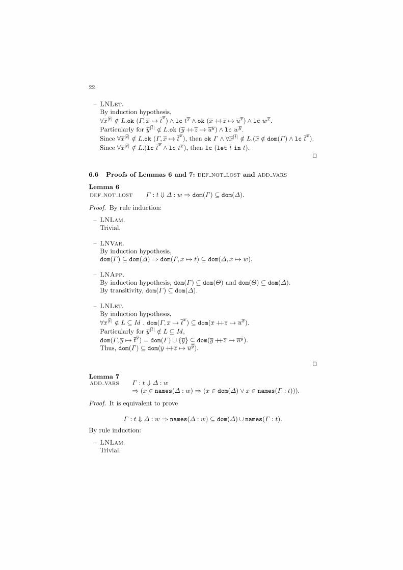
22
– LNLet.By induction hypothesis,
∀x|t| /∈ L.ok (Γ, x 7→ tx) ∧ lc tx ∧ ok (x++z 7→ ux) ∧ lc wx.
Particularly for y|t| /∈ L.ok (y ++z 7→ uy) ∧ lc wy.
Since ∀x|t| /∈ L.ok (Γ, x 7→ tx), then ok Γ ∧ ∀x|t| /∈ L.(x /∈ dom(Γ ) ∧ lc tx).
Since ∀x|t| /∈ L.(lc tx ∧ lc tx), then lc (let t in t).ut
6.6 Proofs of Lemmas 6 and 7: def not lost and add vars
Lemma 6def not lost Γ : t ⇓ ∆ : w ⇒ dom(Γ ) ⊆ dom(∆).
Proof. By rule induction:
– LNLam.Trivial.
– LNVar.By induction hypothesis,dom(Γ ) ⊆ dom(∆)⇒ dom(Γ, x 7→ t) ⊆ dom(∆,x 7→ w).
– LNApp.By induction hypothesis, dom(Γ ) ⊆ dom(Θ) and dom(Θ) ⊆ dom(∆).By transitivity, dom(Γ ) ⊆ dom(∆).
– LNLet.By induction hypothesis,
∀x|t| /∈ L ⊆ Id . dom(Γ, x 7→ tx) ⊆ dom(x++z 7→ ux).
Particularly for y|t| /∈ L ⊆ Id ,
dom(Γ, y 7→ ty) = dom(Γ ) ∪ {y} ⊆ dom(y ++z 7→ uy).
Thus, dom(Γ ) ⊆ dom(y ++z 7→ uy).
ut
Lemma 7add vars Γ : t ⇓ ∆ : w
⇒ (x ∈ names(∆ : w)⇒ (x ∈ dom(∆) ∨ x ∈ names(Γ : t))).
Proof. It is equivalent to prove
Γ : t ⇓ ∆ : w ⇒ names(∆ : w) ⊆ dom(∆) ∪ names(Γ : t).
By rule induction:
– LNLam.Trivial.
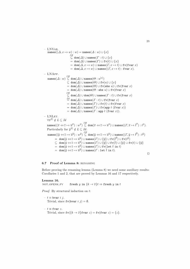
23
– LNVar.names((∆,x 7→ w) : w) = names(∆ : w) ∪ {x}
IH⊆ dom(∆) ∪ names(Γ : t) ∪ {x}= dom(∆) ∪ names(Γ ) ∪ fv(t) ∪ {x}= dom(∆,x 7→ w) ∪ names(Γ, x 7→ t) ∪ fv(fvar x)= dom(∆,x 7→ w) ∪ names((Γ, x 7→ t) : fvar x).
– LNApp.
names(∆ : w)IH⊆ dom(∆) ∪ names(Θ : u[x])⊆ dom(∆) ∪ names(Θ) ∪ fv(u) ∪ {x}= dom(∆) ∪ names(Θ) ∪ fv(abs u) ∪ fv(fvar x)= dom(∆) ∪ names(Θ : abs u) ∪ fv(fvar x)IH⊆ dom(∆) ∪ dom(Θ) ∪ names(Γ : t) ∪ fv(fvar x)L6= dom(∆) ∪ names(Γ : t) ∪ fv(fvar x)= dom(∆) ∪ names(Γ ) ∪ fv(t) ∪ fv(fvar x)= dom(∆) ∪ names(Γ ) ∪ fv(app t (fvar x))= dom(∆) ∪ names(Γ : app t (fvar x)).
– LNLet.∀x|t| /∈ L ⊆ Id
names((x++z 7→ ux) : wx)IH⊆ dom(x++z 7→ ux) ∪ names((Γ, x 7→ t
x) : tx).
Particularly for y|t| /∈ L ⊆ Id :
names((y ++z 7→ uy) : wy)IH⊆ dom(y ++z 7→ uy) ∪ names((Γ, y 7→ t
y) : ty)
= dom(y ++z 7→ uy) ∪ names(Γ ) ∪ {y} ∪ fv(ty) ∪ fv(ty)
⊆ dom(y ++z 7→ uy) ∪ names(Γ ) ∪ {y} ∪ fv(t) ∪ {y} ∪ fv(t) ∪ {y}= dom(y ++z 7→ uy) ∪ names(Γ ) ∪ fv(let t in t)= dom(y ++z 7→ uy) ∪ names(Γ : let t in t).
ut
6.7 Proof of Lemma 8: renaming
Before proving the renaming lemma (Lemma 8) we need some auxiliary results:Corollaries 1 and 2, that are proved by Lemmas 16 and 17 respectively.
Lemma 16.not openk fv fresh y in {k → x}t⇒ fresh y in t
Proof. By structural induction on t:
– t ≡ bvar i j.Trivial, since fv(bvar i j) = ∅.
– t ≡ fvar z.Trivial, since fv({k → x}fvar z) = fv(fvar z) = {z}.
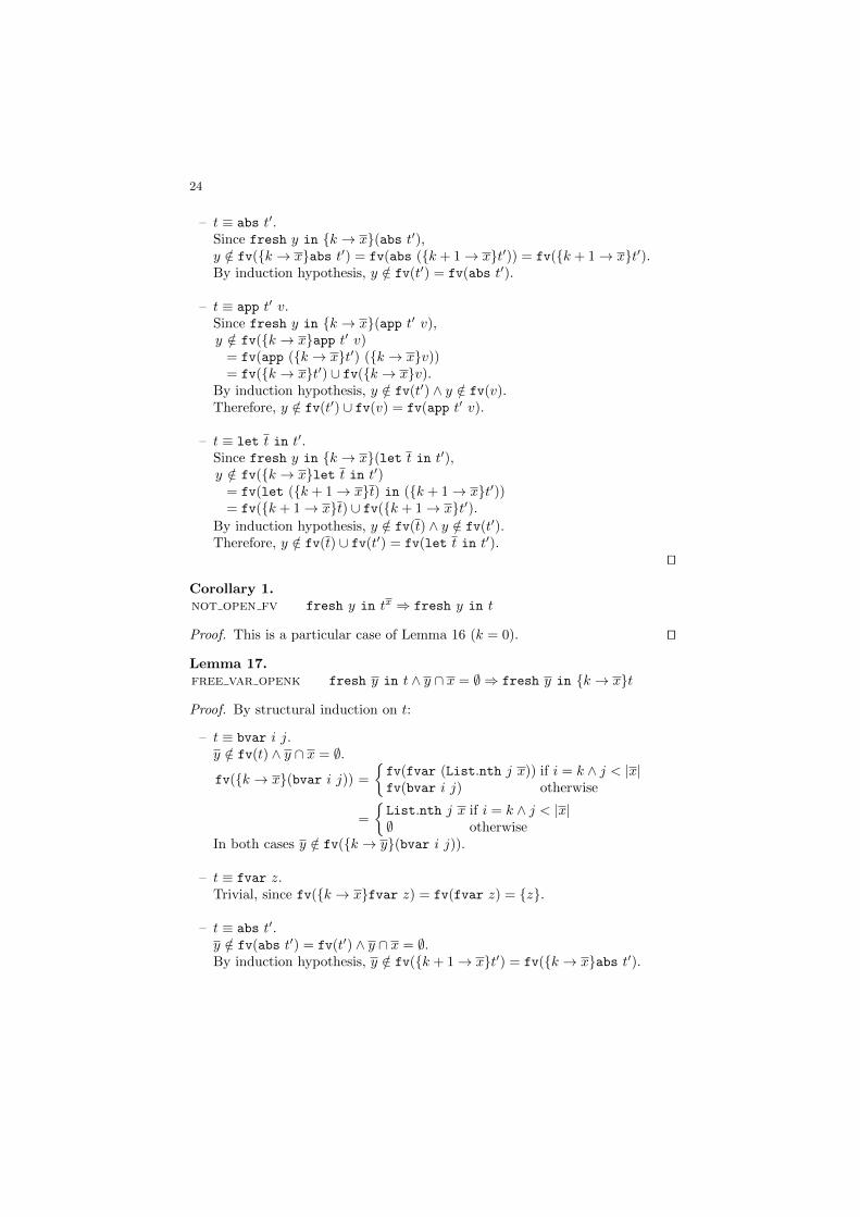
24
– t ≡ abs t′.Since fresh y in {k → x}(abs t′),y /∈ fv({k → x}abs t′) = fv(abs ({k + 1→ x}t′)) = fv({k + 1→ x}t′).By induction hypothesis, y /∈ fv(t′) = fv(abs t′).
– t ≡ app t′ v.Since fresh y in {k → x}(app t′ v),y /∈ fv({k → x}app t′ v)
= fv(app ({k → x}t′) ({k → x}v))= fv({k → x}t′) ∪ fv({k → x}v).
By induction hypothesis, y /∈ fv(t′) ∧ y /∈ fv(v).Therefore, y /∈ fv(t′) ∪ fv(v) = fv(app t′ v).
– t ≡ let t in t′.Since fresh y in {k → x}(let t in t′),y /∈ fv({k → x}let t in t′)
= fv(let ({k + 1→ x}t) in ({k + 1→ x}t′))= fv({k + 1→ x}t) ∪ fv({k + 1→ x}t′).
By induction hypothesis, y /∈ fv(t) ∧ y /∈ fv(t′).Therefore, y /∈ fv(t) ∪ fv(t′) = fv(let t in t′).
ut
Corollary 1.not open fv fresh y in tx ⇒ fresh y in t
Proof. This is a particular case of Lemma 16 (k = 0). ut
Lemma 17.free var openk fresh y in t ∧ y ∩ x = ∅ ⇒ fresh y in {k → x}t
Proof. By structural induction on t:
– t ≡ bvar i j.y /∈ fv(t) ∧ y ∩ x = ∅.fv({k → x}(bvar i j)) =
{fv(fvar (List.nth j x)) if i = k ∧ j < |x|fv(bvar i j) otherwise
=
{List.nth j x if i = k ∧ j < |x|∅ otherwise
In both cases y /∈ fv({k → y}(bvar i j)).
– t ≡ fvar z.Trivial, since fv({k → x}fvar z) = fv(fvar z) = {z}.
– t ≡ abs t′.y /∈ fv(abs t′) = fv(t′) ∧ y ∩ x = ∅.By induction hypothesis, y /∈ fv({k + 1→ x}t′) = fv({k → x}abs t′).
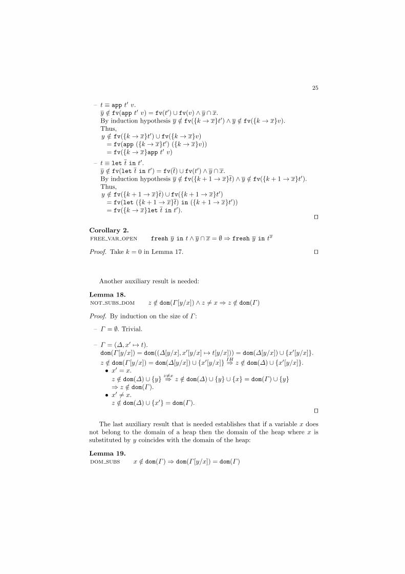
25
– t ≡ app t′ v.y /∈ fv(app t′ v) = fv(t′) ∪ fv(v) ∧ y ∩ x.By induction hypothesis y /∈ fv({k → x}t′) ∧ y /∈ fv({k → x}v).Thus,y /∈ fv({k → x}t′) ∪ fv({k → x}v)
= fv(app ({k → x}t′) ({k → x}v))= fv({k → x}app t′ v)
– t ≡ let t in t′.y /∈ fv(let t in t′) = fv(t) ∪ fv(t′) ∧ y ∩ x.By induction hypothesis y /∈ fv({k + 1→ x}t) ∧ y /∈ fv({k + 1→ x}t′).Thus,y /∈ fv({k + 1→ x}t) ∪ fv({k + 1→ x}t′)
= fv(let ({k + 1→ x}t) in ({k + 1→ x}t′))= fv({k → x}let t in t′).
ut
Corollary 2.free var open fresh y in t ∧ y ∩ x = ∅ ⇒ fresh y in tx
Proof. Take k = 0 in Lemma 17. ut
Another auxiliary result is needed:
Lemma 18.not subs dom z /∈ dom(Γ [y/x]) ∧ z 6= x⇒ z /∈ dom(Γ )
Proof. By induction on the size of Γ :
– Γ = ∅. Trivial.
– Γ = (∆,x′ 7→ t).dom(Γ [y/x]) = dom((∆[y/x], x′[y/x] 7→ t[y/x])) = dom(∆[y/x]) ∪ {x′[y/x]}.z /∈ dom(Γ [y/x]) = dom(∆[y/x]) ∪ {x′[y/x]} IH⇒ z /∈ dom(∆) ∪ {x′[y/x]}.• x′ = x.
z /∈ dom(∆) ∪ {y} z 6=x⇒ z /∈ dom(∆) ∪ {y} ∪ {x} = dom(Γ ) ∪ {y}⇒ z /∈ dom(Γ ).
• x′ 6= x.z /∈ dom(∆) ∪ {x′} = dom(Γ ).
ut
The last auxiliary result that is needed establishes that if a variable x doesnot belong to the domain of a heap then the domain of the heap where x issubstituted by y coincides with the domain of the heap:
Lemma 19.dom subs x /∈ dom(Γ )⇒ dom(Γ [y/x]) = dom(Γ )
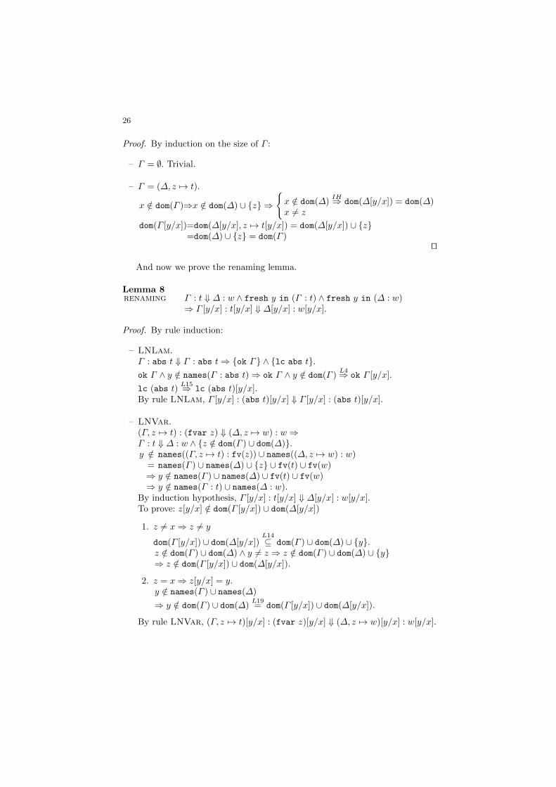
26
Proof. By induction on the size of Γ :
– Γ = ∅. Trivial.
– Γ = (∆, z 7→ t).
x /∈ dom(Γ )⇒x /∈ dom(∆) ∪ {z} ⇒{x /∈ dom(∆)
IH⇒ dom(∆[y/x]) = dom(∆)x 6= z
dom(Γ [y/x])=dom(∆[y/x], z 7→ t[y/x]) = dom(∆[y/x]) ∪ {z}=dom(∆) ∪ {z} = dom(Γ )
ut
And now we prove the renaming lemma.
Lemma 8renaming Γ : t ⇓ ∆ : w ∧ fresh y in (Γ : t) ∧ fresh y in (∆ : w)
⇒ Γ [y/x] : t[y/x] ⇓ ∆[y/x] : w[y/x].
Proof. By rule induction:
– LNLam.Γ : abs t ⇓ Γ : abs t⇒ {ok Γ} ∧ {lc abs t}.ok Γ ∧ y /∈ names(Γ : abs t)⇒ ok Γ ∧ y /∈ dom(Γ )
L4⇒ ok Γ [y/x].
lc (abs t)L15⇒ lc (abs t)[y/x].
By rule LNLam, Γ [y/x] : (abs t)[y/x] ⇓ Γ [y/x] : (abs t)[y/x].
– LNVar.(Γ, z 7→ t) : (fvar z) ⇓ (∆, z 7→ w) : w ⇒Γ : t ⇓ ∆ : w ∧ {z /∈ dom(Γ ) ∪ dom(∆)}.y /∈ names((Γ, z 7→ t) : fv(z)) ∪ names((∆, z 7→ w) : w)
= names(Γ ) ∪ names(∆) ∪ {z} ∪ fv(t) ∪ fv(w)⇒ y /∈ names(Γ ) ∪ names(∆) ∪ fv(t) ∪ fv(w)⇒ y /∈ names(Γ : t) ∪ names(∆ : w).
By induction hypothesis, Γ [y/x] : t[y/x] ⇓ ∆[y/x] : w[y/x].To prove: z[y/x] /∈ dom(Γ [y/x]) ∪ dom(∆[y/x])
1. z 6= x⇒ z 6= y
dom(Γ [y/x]) ∪ dom(∆[y/x])L14⊆ dom(Γ ) ∪ dom(∆) ∪ {y}.
z /∈ dom(Γ ) ∪ dom(∆) ∧ y 6= z ⇒ z /∈ dom(Γ ) ∪ dom(∆) ∪ {y}⇒ z /∈ dom(Γ [y/x]) ∪ dom(∆[y/x]).
2. z = x⇒ z[y/x] = y.y /∈ names(Γ ) ∪ names(∆)
⇒ y /∈ dom(Γ ) ∪ dom(∆)L19= dom(Γ [y/x]) ∪ dom(∆[y/x]).
By rule LNVar, (Γ, z 7→ t)[y/x] : (fvar z)[y/x] ⇓ (∆, z 7→ w)[y/x] : w[y/x].
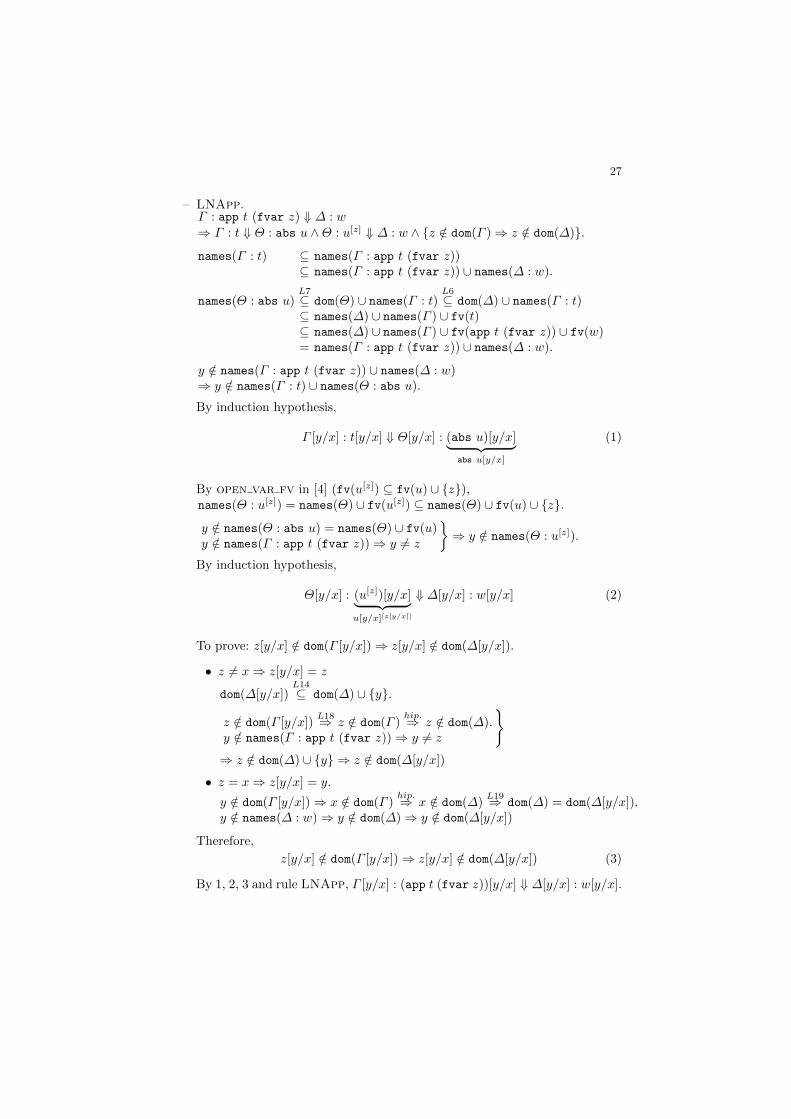
27
– LNApp.Γ : app t (fvar z) ⇓ ∆ : w⇒ Γ : t ⇓ Θ : abs u ∧Θ : u[z] ⇓ ∆ : w ∧ {z /∈ dom(Γ )⇒ z /∈ dom(∆)}.names(Γ : t) ⊆ names(Γ : app t (fvar z))
⊆ names(Γ : app t (fvar z)) ∪ names(∆ : w).
names(Θ : abs u)L7⊆ dom(Θ) ∪ names(Γ : t)
L6⊆ dom(∆) ∪ names(Γ : t)
⊆ names(∆) ∪ names(Γ ) ∪ fv(t)⊆ names(∆) ∪ names(Γ ) ∪ fv(app t (fvar z)) ∪ fv(w)= names(Γ : app t (fvar z)) ∪ names(∆ : w).
y /∈ names(Γ : app t (fvar z)) ∪ names(∆ : w)⇒ y /∈ names(Γ : t) ∪ names(Θ : abs u).
By induction hypothesis,
Γ [y/x] : t[y/x] ⇓ Θ[y/x] : (abs u)[y/x]︸ ︷︷ ︸abs u[y/x]
(1)
By open var fv in [4] (fv(u[z]) ⊆ fv(u) ∪ {z}),names(Θ : u[z]) = names(Θ) ∪ fv(u[z]) ⊆ names(Θ) ∪ fv(u) ∪ {z}.y /∈ names(Θ : abs u) = names(Θ) ∪ fv(u)y /∈ names(Γ : app t (fvar z))⇒ y 6= z
}⇒ y /∈ names(Θ : u[z]).
By induction hypothesis,
Θ[y/x] : (u[z])[y/x]︸ ︷︷ ︸u[y/x][z[y/x]]
⇓ ∆[y/x] : w[y/x] (2)
To prove: z[y/x] /∈ dom(Γ [y/x])⇒ z[y/x] /∈ dom(∆[y/x]).
• z 6= x⇒ z[y/x] = z
dom(∆[y/x])L14⊆ dom(∆) ∪ {y}.
z /∈ dom(Γ [y/x])L18⇒ z /∈ dom(Γ )
hip.⇒ z /∈ dom(∆).y /∈ names(Γ : app t (fvar z))⇒ y 6= z
}
⇒ z /∈ dom(∆) ∪ {y} ⇒ z /∈ dom(∆[y/x])
• z = x⇒ z[y/x] = y.
y /∈ dom(Γ [y/x])⇒ x /∈ dom(Γ )hip.⇒ x /∈ dom(∆)
L19⇒ dom(∆) = dom(∆[y/x]).y /∈ names(∆ : w)⇒ y /∈ dom(∆)⇒ y /∈ dom(∆[y/x])
Therefore,
z[y/x] /∈ dom(Γ [y/x])⇒ z[y/x] /∈ dom(∆[y/x]) (3)
By 1, 2, 3 and rule LNApp, Γ [y/x] : (app t (fvar z))[y/x] ⇓ ∆[y/x] : w[y/x].
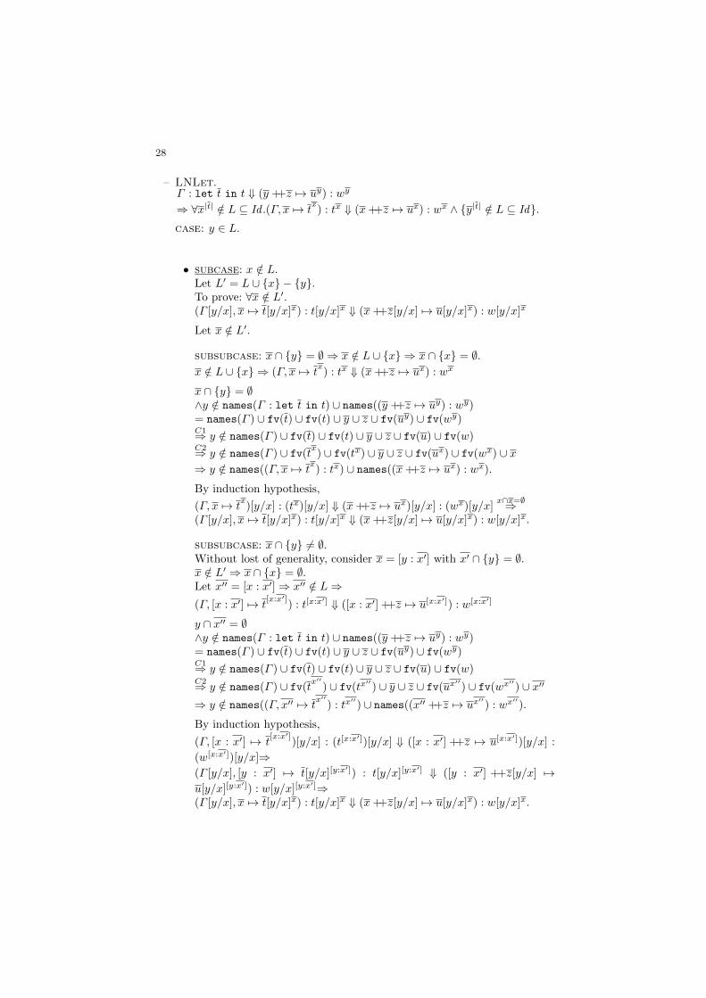
28
– LNLet.Γ : let t in t ⇓ (y ++z 7→ uy) : wy
⇒ ∀x|t| /∈ L ⊆ Id .(Γ, x 7→ tx) : tx ⇓ (x++z 7→ ux) : wx ∧ {y|t| /∈ L ⊆ Id}.
case: y ∈ L.
• subcase: x /∈ L.Let L′ = L ∪ {x} − {y}.To prove: ∀x /∈ L′.(Γ [y/x], x 7→ t[y/x]x) : t[y/x]x ⇓ (x++z[y/x] 7→ u[y/x]x) : w[y/x]x
Let x /∈ L′.
subsubcase: x ∩ {y} = ∅ ⇒ x /∈ L ∪ {x} ⇒ x ∩ {x} = ∅.x /∈ L ∪ {x} ⇒ (Γ, x 7→ t
x) : tx ⇓ (x++z 7→ ux) : wx
x ∩ {y} = ∅∧y /∈ names(Γ : let t in t) ∪ names((y ++z 7→ uy) : wy)= names(Γ ) ∪ fv(t) ∪ fv(t) ∪ y ∪ z ∪ fv(uy) ∪ fv(wy)C1⇒ y /∈ names(Γ ) ∪ fv(t) ∪ fv(t) ∪ y ∪ z ∪ fv(u) ∪ fv(w)C2⇒ y /∈ names(Γ ) ∪ fv(t
x) ∪ fv(tx) ∪ y ∪ z ∪ fv(ux) ∪ fv(wx) ∪ x
⇒ y /∈ names((Γ, x 7→ tx) : tx) ∪ names((x++z 7→ ux) : wx).
By induction hypothesis,
(Γ, x 7→ tx)[y/x] : (tx)[y/x] ⇓ (x++z 7→ ux)[y/x] : (wx)[y/x]
x∩x=∅⇒(Γ [y/x], x 7→ t[y/x]x) : t[y/x]x ⇓ (x++z[y/x] 7→ u[y/x]x) : w[y/x]x.
subsubcase: x ∩ {y} 6= ∅.Without lost of generality, consider x = [y : x′] with x′ ∩ {y} = ∅.x /∈ L′ ⇒ x ∩ {x} = ∅.Let x′′ = [x : x′]⇒ x′′ /∈ L⇒(Γ, [x : x′] 7→ t
[x:x′]) : t[x:x
′] ⇓ ([x : x′] ++z 7→ u[x:x′]) : w[x:x′]
y ∩ x′′ = ∅∧y /∈ names(Γ : let t in t) ∪ names((y ++z 7→ uy) : wy)= names(Γ ) ∪ fv(t) ∪ fv(t) ∪ y ∪ z ∪ fv(uy) ∪ fv(wy)C1⇒ y /∈ names(Γ ) ∪ fv(t) ∪ fv(t) ∪ y ∪ z ∪ fv(u) ∪ fv(w)C2⇒ y /∈ names(Γ ) ∪ fv(t
x′′) ∪ fv(tx
′′) ∪ y ∪ z ∪ fv(ux
′′) ∪ fv(wx′′
) ∪ x′′⇒ y /∈ names((Γ, x′′ 7→ t
x′′) : tx
′′) ∪ names((x′′ ++z 7→ ux
′′) : wx′′
).
By induction hypothesis,
(Γ, [x : x′] 7→ t[x:x′]
)[y/x] : (t[x:x′])[y/x] ⇓ ([x : x′] ++z 7→ u[x:x
′])[y/x] :
(w[x:x′])[y/x]⇒(Γ [y/x], [y : x′] 7→ t[y/x][y:x
′]) : t[y/x][y:x′] ⇓ ([y : x′] ++z[y/x] 7→
u[y/x][y:x′]) : w[y/x][y:x
′]⇒(Γ [y/x], x 7→ t[y/x]x) : t[y/x]x ⇓ (x++z[y/x] 7→ u[y/x]x) : w[y/x]x.
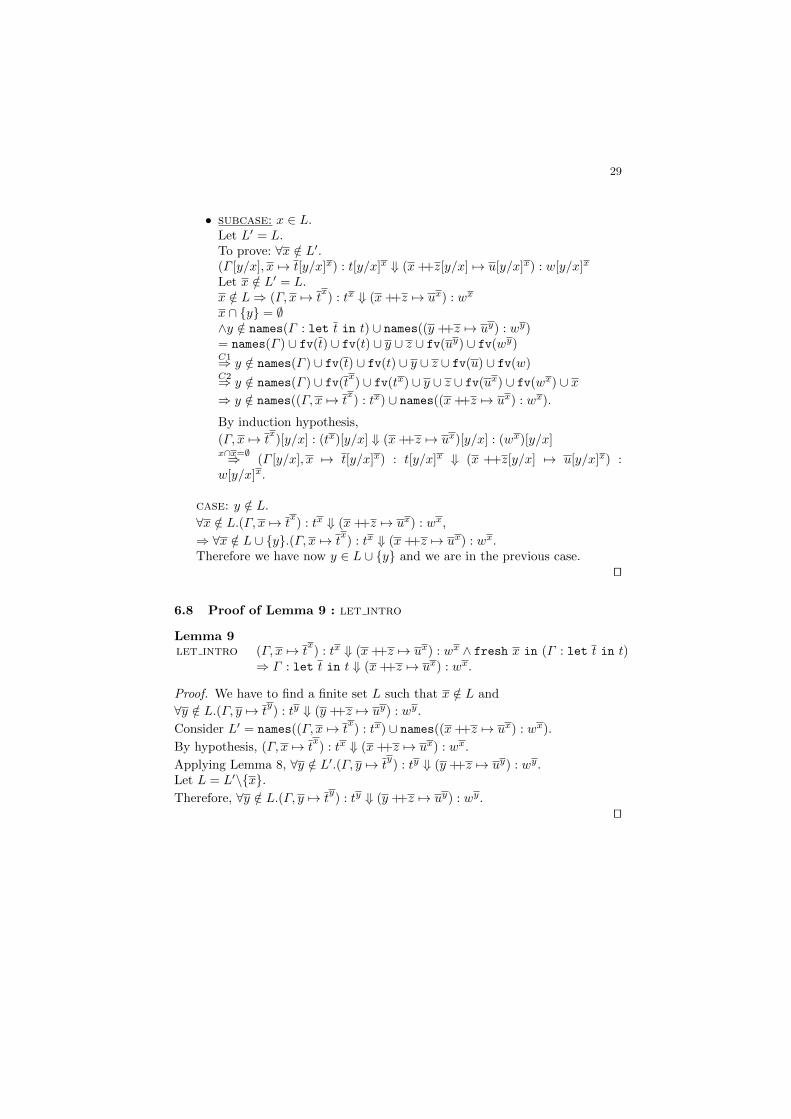
29
• subcase: x ∈ L.Let L′ = L.To prove: ∀x /∈ L′.(Γ [y/x], x 7→ t[y/x]x) : t[y/x]x ⇓ (x++z[y/x] 7→ u[y/x]x) : w[y/x]x
Let x /∈ L′ = L.x /∈ L⇒ (Γ, x 7→ t
x) : tx ⇓ (x++z 7→ ux) : wx
x ∩ {y} = ∅∧y /∈ names(Γ : let t in t) ∪ names((y ++z 7→ uy) : wy)= names(Γ ) ∪ fv(t) ∪ fv(t) ∪ y ∪ z ∪ fv(uy) ∪ fv(wy)C1⇒ y /∈ names(Γ ) ∪ fv(t) ∪ fv(t) ∪ y ∪ z ∪ fv(u) ∪ fv(w)C2⇒ y /∈ names(Γ ) ∪ fv(t
x) ∪ fv(tx) ∪ y ∪ z ∪ fv(ux) ∪ fv(wx) ∪ x
⇒ y /∈ names((Γ, x 7→ tx) : tx) ∪ names((x++z 7→ ux) : wx).
By induction hypothesis,
(Γ, x 7→ tx)[y/x] : (tx)[y/x] ⇓ (x++z 7→ ux)[y/x] : (wx)[y/x]
x∩x=∅⇒ (Γ [y/x], x 7→ t[y/x]x) : t[y/x]x ⇓ (x ++z[y/x] 7→ u[y/x]x) :w[y/x]x.
case: y /∈ L.
∀x /∈ L.(Γ, x 7→ tx) : tx ⇓ (x++z 7→ ux) : wx,
⇒ ∀x /∈ L ∪ {y}.(Γ, x 7→ tx) : tx ⇓ (x++z 7→ ux) : wx.
Therefore we have now y ∈ L ∪ {y} and we are in the previous case.ut
6.8 Proof of Lemma 9 : let intro
Lemma 9let intro (Γ, x 7→ t
x) : tx ⇓ (x++z 7→ ux) : wx ∧ fresh x in (Γ : let t in t)
⇒ Γ : let t in t ⇓ (x++z 7→ ux) : wx.
Proof. We have to find a finite set L such that x /∈ L and
∀y /∈ L.(Γ, y 7→ ty) : ty ⇓ (y ++z 7→ uy) : wy.
Consider L′ = names((Γ, x 7→ tx) : tx) ∪ names((x++z 7→ ux) : wx).
By hypothesis, (Γ, x 7→ tx) : tx ⇓ (x++z 7→ ux) : wx.
Applying Lemma 8, ∀y /∈ L′.(Γ, y 7→ ty) : ty ⇓ (y ++z 7→ uy) : wy.
Let L = L′\{x}.Therefore, ∀y /∈ L.(Γ, y 7→ t
y) : ty ⇓ (y ++z 7→ uy) : wy.
ut

198 Capıtulo A. Versiones extendidas
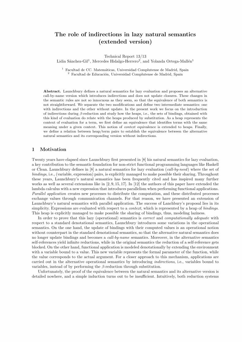
The role of indirections in lazy natural semantics(extended version)
Technical Report 13/13Lidia Sanchez-Gil1, Mercedes Hidalgo-Herrero2, and Yolanda Ortega-Mallen1
1 Facultad de CC. Matematicas, Universidad Complutense de Madrid, Spain2 Facultad de Educacion, Universidad Complutense de Madrid, Spain
Abstract. Launchbury defines a natural semantics for lazy evaluation and proposes an alternativecall-by-name version which introduces indirections and does not update closures. These changes inthe semantic rules are not so innocuous as they seem, so that the equivalence of both semantics isnot straightforward. We separate the two modifications and define two intermediate semantics: onewith indirections and the other without update. In the present work we focus on the introductionof indirections during β-reduction and study how the heaps, i.e., the sets of bindings, obtained withthis kind of evaluation do relate with the heaps produced by substitution. As a heap represents thecontext of evaluation for a term, we first define an equivalence that identifies terms with the samemeaning under a given context. This notion of context equivalence is extended to heaps. Finally,we define a relation between heap/term pairs to establish the equivalence between the alternativenatural semantics and its corresponding version without indirections.
1 Motivation
Twenty years have elapsed since Launchbury first presented in [8] his natural semantics for lazy evaluation,a key contribution to the semantic foundation for non-strict functional programming languages like Haskellor Clean. Launchbury defines in [8] a natural semantics for lazy evaluation (call-by-need) where the set ofbindings, i.e., (variable, expression) pairs, is explicitly managed to make possible their sharing. Throughoutthese years, Launchbury’s natural semantics has been frequently cited and has inspired many furtherworks as well as several extensions like in [2, 9, 15, 17]. In [12] the authors of this paper have extended thelambda calculus with a new expression that introduces parallelism when performing functional applications.Parallel application creates new processes to distribute the computation, and these distributed processesexchange values through communication channels. For that reason, we have presented an extension ofLaunchbury’s natural semantics with parallel application. The success of Lanchbury’s proposal lies in itssimplicity. Expressions are evaluated with respect to a context, which is represented by a heap of bindings.This heap is explicitly managed to make possible the sharing of bindings, thus, modeling laziness.
In order to prove that this lazy (operational) semantics is correct and computationally adequate withrespect to a standard denotational semantics, Launchbury introduces some variations in the operationalsemantics. On the one hand, the update of bindings with their computed values is an operational notionwithout counterpart in the standard denotational semantics, so that the alternative natural semantics doesno longer update bindings and becomes a call-by-name semantics. Moreover, in the alternative semanticsself-references yield infinite reductions, while in the original semantics the reduction of a self-reference getsblocked. On the other hand, functional application is modeled denotationally by extending the environmentwith a variable bound to a value. This new variable represents the formal parameter of the function, whilethe value corresponds to the actual argument. For a closer approach to this mechanism, applications arecarried out in the alternative operational semantics by introducing indirections, i.e., variables bound tovariables, instead of by performing the β-reduction through substitution.
Unfortunately, the proof of the equivalence between the natural semantics and its alternative version isdetailed nowhere, and a simple induction turns out to be insufficient. Intuitively, both reduction systems

2
should lead to the same results. However, the context-heap semantics is too sensitive to the changesintroduced by the alternative rules. Consequently, the equivalence cannot be directly established since finalvalues may contain free variables that are dependent on the context of evaluation, which is representedby the heap of bindings. No updating leads to the duplication of bindings, and although these duplicatedbindings, as well as the indirections, do not add relevant information to the context, it is awkward to provethis fact. Therefore, our challenge is to establish a way of relating the heaps obtained with each reductionsystem, and to prove that at the end the semantics are equivalent, so that any reduction of a term in one ofthe systems has its counterpart in the other. To facilitate this task we consider separately the no updatingand the introduction of indirections, and we define two intermediate semantics.
In this paper we investigate the effect of introducing indirections in a setting without updates, and weanalyze the similarities and differences between the reductions proofs obtained with and without indirec-tions. This analysis provides a deep insight on the behavior of a context-heap semantics like Launchbury’s.
We want to identify terms up to α-conversion, but dealing with α-equated terms usually implies theuse of Barendregt’s variable convention [3] to avoid the renaming of bound variables. However, the useof the variable convention is sometimes dubious and may lead to faulty results (as it is shown by Urbanet al. in [16]). Moreover, we intend to formalize our results with the help of the Coq [4] proof assistant.These reasons have led us to look for a system of binding amenable to formalization and we have chosen alocally nameless representation (as presented by Chargueraud in [6]). This is a mixed notation where boundvariables names are replaced by de Bruijn indices [7], while free variables preserve their names. Althoughde Bruijn indices solve the problem with α-conversion, they make it very complicated to deal with heaps.Moreover, the formalization becomes unreadable. Hence, the mixed notation of naming variables is moreconvenient. A locally nameless version of Launchbury’s natural semantics has been presented by the authorsin [14] and [13].
The main contributions of the present work are:
1. An equivalence relation that identifies heaps that define the same free variables but whose correspond-ing closures may differ on undefined free variables ;
2. A preorder that relates two heaps whenever the first can be transformed into the second by eliminatingindirections ;
3. An extension of the preorder relation for heap/term pairs expressing that two terms are equivalent ifthey have the same structure and their free variables, defined in the context of the respective heaps,are the same except for some indirections.
4. An equivalence theorem for Launchbury’s alternative semantics and a version without indirections(and without update).
The paper is structured as follows: In Section 2, we review the lambda calculus and the two naturalsemantics described by Launchbury in [8]. We also introduce two intermediate semantics, each introducingjust one alternative rule. In Section 3 we give a locally nameless representation of the calculus and thesemantics presented in Section 2. In Section 4 we define equivalence and preorder relations on terms, heapsand also on heap/term pairs. We include a number of interesting results concerning these relations and,finally, we prove the equivalence of Launchbury’s alternative semantics and the intermediate semanticswithout update and without indirections. In the last section we draw conclusions and outline our futurework.
The proofs of theorems, propositions and lemmas are detailed in the Appendix.
2 Lazy natural semantics
In this section we review the natural semantics defined by Launchbury in [8] for lazy evaluation, togetherwith the alternative rules for application and variables which transform the lazy semantics in a call-by-name semantics. In order to facilitate the comparison of these semantics, we focus independently on eachchange and define two intermediate semantics.
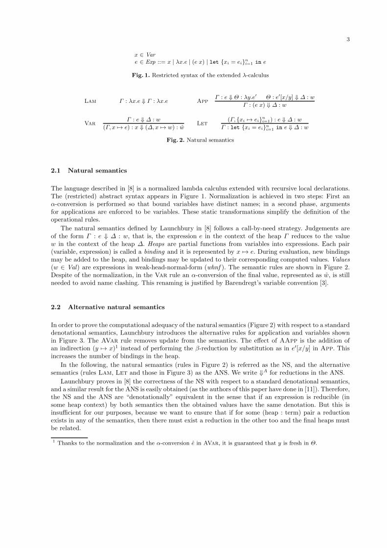
3
x ∈ Vare ∈ Exp ::= x | λx.e | (e x) | let {xi = ei}ni=1 in e
Fig. 1. Restricted syntax of the extended λ-calculus
Lam Γ : λx.e ⇓ Γ : λx.e AppΓ : e ⇓ Θ : λy.e′ Θ : e′[x/y] ⇓ ∆ : w
Γ : (e x) ⇓ ∆ : w
VarΓ : e ⇓ ∆ : w
(Γ, x 7→ e) : x ⇓ (∆,x 7→ w) : wLet
(Γ, {xi 7→ ei}ni=1) : e ⇓ ∆ : w
Γ : let {xi = ei}ni=1 in e ⇓ ∆ : w
Fig. 2. Natural semantics
2.1 Natural semantics
The language described in [8] is a normalized lambda calculus extended with recursive local declarations.The (restricted) abstract syntax appears in Figure 1. Normalization is achieved in two steps: First anα-conversion is performed so that bound variables have distinct names; in a second phase, argumentsfor applications are enforced to be variables. These static transformations simplify the definition of theoperational rules.
The natural semantics defined by Launchbury in [8] follows a call-by-need strategy. Judgements areof the form Γ : e ⇓ ∆ : w, that is, the expression e in the context of the heap Γ reduces to the valuew in the context of the heap ∆. Heaps are partial functions from variables into expressions. Each pair(variable, expression) is called a binding and it is represented by x 7→ e. During evaluation, new bindingsmay be added to the heap, and bindings may be updated to their corresponding computed values. Values(w ∈ Val) are expressions in weak-head-normal-form (whnf ). The semantic rules are shown in Figure 2.Despite of the normalization, in the Var rule an α-conversion of the final value, represented as w, is stillneeded to avoid name clashing. This renaming is justified by Barendregt’s variable convention [3].
2.2 Alternative natural semantics
In order to prove the computational adequacy of the natural semantics (Figure 2) with respect to a standarddenotational semantics, Launchbury introduces the alternative rules for application and variables shownin Figure 3. The AVar rule removes update from the semantics. The effect of AApp is the addition ofan indirection (y 7→ x)1 instead of performing the β-reduction by substitution as in e′[x/y] in App. Thisincreases the number of bindings in the heap.
In the following, the natural semantics (rules in Figure 2) is referred as the NS, and the alternativesemantics (rules Lam, Let and those in Figure 3) as the ANS. We write ⇓A for reductions in the ANS.
Launchbury proves in [8] the correctness of the NS with respect to a standard denotational semantics,and a similar result for the ANS is easily obtained (as the authors of this paper have done in [11]). Therefore,the NS and the ANS are “denotationally” equivalent in the sense that if an expression is reducible (insome heap context) by both semantics then the obtained values have the same denotation. But this isinsufficient for our purposes, because we want to ensure that if for some (heap : term) pair a reductionexists in any of the semantics, then there must exist a reduction in the other too and the final heaps mustbe related.
1 Thanks to the normalization and the α-conversion e in AVar, it is guaranteed that y is fresh in Θ.
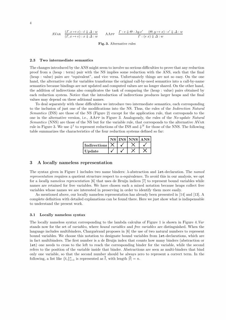
4
AVar(Γ, x 7→ e) : e ⇓ ∆ : w
(Γ, x 7→ e) : x ⇓ ∆ : wAApp
Γ : e ⇓ Θ : λy.e′ (Θ, y 7→ x) : e′ ⇓ ∆ : w
Γ : (e x) ⇓ ∆ : w
Fig. 3. Alternative rules
2.3 Two intermediate semantics
The changes introduced by the ANS might seem to involve no serious difficulties to prove that any reductionproof from a (heap : term) pair with the NS implies some reduction with the ANS, such that the final(heap : value) pairs are “equivalent”, and vice versa. Unfortunately things are not so easy. On the onehand, the alternative rule for variables transforms the original call-by-need semantics into a call-by-namesemantics because bindings are not updated and computed values are no longer shared. On the other hand,the addition of indirections also complicates the task of comparing the (heap : value) pairs obtained byeach reduction system. Notice that the introduction of indirections produces larger heaps and the finalvalues may depend on these aditional names.
To deal separately with these difficulties we introduce two intermediate semantics, each correspondingto the inclusion of just one of the modifications into the NS. Thus, the rules of the Indirection NaturalSemantics (INS) are those of the NS (Figure 2) except for the application rule, that corresponds to theone in the alternative version, i.e., AApp in Figure 3. Analogously, the rules of the No-update NaturalSemantics (NNS) are those of the NS but for the variable rule, that corresponds to the alternative AVarrule in Figure 3. We use ⇓I to represent reductions of the INS and ⇓N for those of the NNS. The followingtable summarizes the characteristics of the four reduction systems defined so far:
NS INS NNS ANS
Indirections # ! # !
Update ! ! # #
3 A locally nameless representation
The syntax given in Figure 1 includes two name binders: λ-abstraction and let-declaration. The namedrepresentation requires a quotient structure respect to α-equivalence. To avoid this in our analysis, we optfor a locally nameless representation [6] that uses de Bruijn indices [7] to represent bound variables whilenames are retained for free variables. We have chosen such a mixed notation because heaps collect freevariables whose names we are interested in preserving in order to identify them more easily.
As mentioned above, our locally nameless representation has already been presented in [14] and [13]. Acomplete definition with detailed explanations can be found there. Here we just show what is indispensableto understand the present work.
3.1 Locally nameless syntax
The locally nameless syntax corresponding to the lambda calculus of Figure 1 is shown in Figure 4.Varstands now for the set of variables, where bound variables and free variables are distinguished. When thelanguage includes multibinders, Chargueraud proposes in [6] the use of two natural numbers to representbound variables. We choose this notation to designate bound variables from let-declarations, which arein fact multibinders. The first number is a de Bruijn index that counts how many binders (abstraction orlet) one needs to cross to the left to reach the corresponding binder for the variable, while the secondrefers to the position of the variable inside that binder. Abstractions are seen as multi-binders that bindonly one variable, so that the second number should be always zero to represent a correct term. In thefollowing, a list like {ti}ni=1 is represented as t, with length |t| = n.
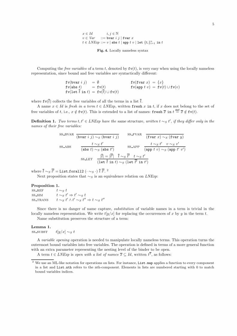
5
x ∈ Id i, j ∈ Nv ∈ Var ::= bvar i j | fvar xt ∈ LNExp ::= v | abs t | app t v | let {ti}ni=1 in t
Fig. 4. Locally nameless syntax
Computing the free variables of a term t, denoted by fv(t), is very easy when using the locally namelessrepresentation, since bound and free variables are syntactically different:
fv(bvar i j) = ∅ fv(fvar x) = {x}fv(abs t) = fv(t) fv(app t v) = fv(t) ∪ fv(v)fv(let t in t) = fv(t) ∪ fv(t)
where fv(t) collects the free variables of all the terms in a list t.
A name x ∈ Id is fresh in a term t ∈ LNExp, written fresh x in t, if x does not belong to the set of
free variables of t, i.e., x /∈ fv(t). This is extended to a list of names: fresh x in tdef= x /∈ fv(t).
Definition 1. Two terms t, t′ ∈ LNExp have the same structure, written t ∼S t′, if they differ only in thenames of their free variables:
ss bvar(bvar i j) ∼S (bvar i j)
ss fvar(fvar x) ∼S (fvar y)
ss abst ∼S t′
(abs t) ∼S (abs t′)ss app
t ∼S t′ v ∼S v′
(app t v) ∼S (app t′ v′)
ss let|t| = |t′| t ∼S t′ t ∼S t′
(let t in t) ∼S (let t′ in t′)
where t ∼S t′ = List.forall2 (· ∼S ·) t t′. 2
Next proposition states that ∼S is an equivalence relation on LNExp:
Proposition 1.ss ref t ∼S tss sim t ∼S t′ ⇒ t′ ∼S tss trans t ∼S t′ ∧ t′ ∼S t′′ ⇒ t ∼S t′′
Since there is no danger of name capture, substitution of variable names in a term is trivial in thelocally nameless representation. We write t[y/x] for replacing the occurrences of x by y in the term t.
Name substitution preserves the structure of a term:
Lemma 1.ss subst t[y/x] ∼S t
A variable opening operation is needed to manipulate locally nameless terms. This operation turns theoutermost bound variables into free variables. The operation is defined in terms of a more general functionwith an extra parameter representing the nesting level of the binder to be open.
A term t ∈ LNExp is open with a list of names x ⊆ Id , written tx, as follows:
2 We use an ML-like notation for operations on lists. For instance, List.map applies a function to every componentin a list and List.nth refers to the nth-component. Elements in lists are numbered starting with 0 to matchbound variables indices.
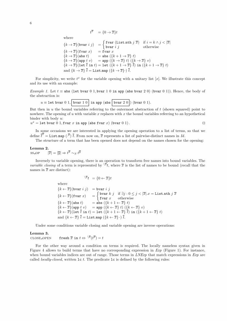
6
tx = {0→ x}twhere
{k→ x}(bvar i j) =
{fvar (List.nth j x) if i = k ∧ j < |x|bvar i j otherwise
{k→ x}(fvar x) = fvar x{k→ x}(abs t) = abs ({k + 1→ x} t){k→ x}(app t v) = app ({k→ x} t) ({k → x} v){k→ x}(let t in t) = let ({k + 1→ x} t) in ({k + 1→ x} t)and {k → x} t = List.map ({k → x}·) t.
For simplicity, we write tx for the variable opening with a unitary list [x]. We illustrate this conceptand its use with an example:
Example 1. Let t ≡ abs (let bvar 0 1, bvar 1 0 in app (abs bvar 2 0) (bvar 0 1)). Hence, the body ofthe abstraction is:
u ≡ let bvar 0 1, bvar 1 0 in app (abs bvar 2 0 ) (bvar 0 1).
But then in u the bound variables referring to the outermost abstraction of t (shown squared) point tonowhere. The opening of u with variable x replaces with x the bound variables referring to an hypotheticalbinder with body u:ux = let bvar 0 1, fvar x in app (abs fvar x) (bvar 0 1) . ⊓⊔
In some occasions we are interested in applying the opening operation to a list of terms, so that we
define tx
= List.map (·x) t. From now on, x represents a list of pairwise-distinct names in Id .The structure of a term that has been opened does not depend on the names chosen for the opening:
Lemma 2.ss op |x| = |y| ⇒ tx ∼S ty
Inversely to variable opening, there is an operation to transform free names into bound variables. Thevariable closing of a term is represented by \xt, where x is the list of names to be bound (recall that thenames in x are distinct):
\xt = {0← x}twhere
{k← x}(bvar i j) = bvar i j
{k← x}(fvar x) =
{bvar k j if ∃j : 0 ≤ j < |x|.x = List.nth j xfvar x otherwise
{k← x}(abs t) = abs ({k + 1← x} t){k← x}(app t v) = app ({k← x} t) ({k ← x} v){k← x}(let t in t) = let ({k + 1← x} t) in ({k + 1← x} t)and {k← x} t = List.map ({k ← x} ·) t.
Under some conditions variable closing and variable opening are inverse operations:
Lemma 3.close open fresh x in t⇔ \x(tx) = t
For the other way around a condition on terms is required. The locally nameless syntax given inFigure 4 allows to build terms that have no corresponding expression in Exp (Figure 1). For instance,when bound variables indices are out of range. Those terms in LNExp that match expressions in Exp arecalled locally-closed, written lc t. The predicate lc is defined by the following rules:
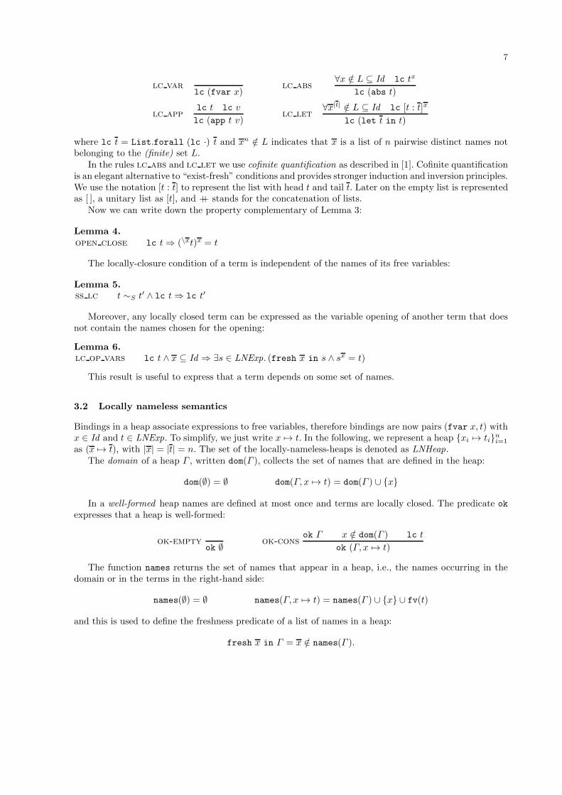
7
lc varlc (fvar x)
lc abs∀x /∈ L ⊆ Id lc tx
lc (abs t)
lc applc t lc v
lc (app t v)lc let
∀x|t| /∈ L ⊆ Id lc [t : t]x
lc (let t in t)
where lc t = List.forall (lc ·) t and xn /∈ L indicates that x is a list of n pairwise distinct names notbelonging to the (finite) set L.
In the rules lc abs and lc let we use cofinite quantification as described in [1]. Cofinite quantificationis an elegant alternative to “exist-fresh” conditions and provides stronger induction and inversion principles.We use the notation [t : t] to represent the list with head t and tail t. Later on the empty list is representedas [ ], a unitary list as [t], and ++ stands for the concatenation of lists.
Now we can write down the property complementary of Lemma 3:
Lemma 4.open close lc t⇒ (\xt)x = t
The locally-closure condition of a term is independent of the names of its free variables:
Lemma 5.ss lc t ∼S t′ ∧ lc t⇒ lc t′
Moreover, any locally closed term can be expressed as the variable opening of another term that doesnot contain the names chosen for the opening:
Lemma 6.lc op vars lc t ∧ x ⊆ Id ⇒ ∃s ∈ LNExp. (fresh x in s ∧ sx = t)
This result is useful to express that a term depends on some set of names.
3.2 Locally nameless semantics
Bindings in a heap associate expressions to free variables, therefore bindings are now pairs (fvar x, t) withx ∈ Id and t ∈ LNExp. To simplify, we just write x 7→ t. In the following, we represent a heap {xi 7→ ti}ni=1
as (x 7→ t), with |x| = |t| = n. The set of the locally-nameless-heaps is denoted as LNHeap.The domain of a heap Γ , written dom(Γ ), collects the set of names that are defined in the heap:
dom(∅) = ∅ dom(Γ, x 7→ t) = dom(Γ ) ∪ {x}
In a well-formed heap names are defined at most once and terms are locally closed. The predicate ok
expresses that a heap is well-formed:
ok-emptyok ∅ ok-cons
ok Γ x /∈ dom(Γ ) lc t
ok (Γ, x 7→ t)
The function names returns the set of names that appear in a heap, i.e., the names occurring in thedomain or in the terms in the right-hand side:
names(∅) = ∅ names(Γ, x 7→ t) = names(Γ ) ∪ {x} ∪ fv(t)
and this is used to define the freshness predicate of a list of names in a heap:
fresh x in Γ = x /∈ names(Γ ).
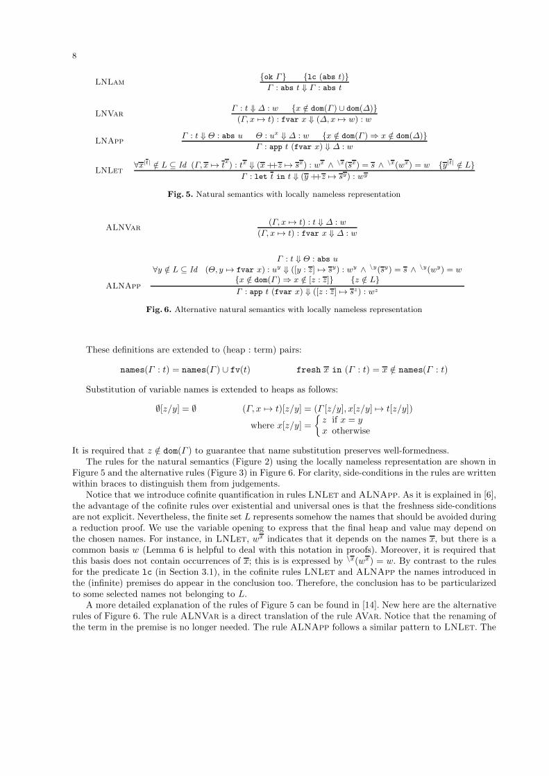
8
LNLam{ok Γ} {lc (abs t)}Γ : abs t ⇓ Γ : abs t
LNVarΓ : t ⇓ ∆ : w {x /∈ dom(Γ ) ∪ dom(∆)}(Γ, x 7→ t) : fvar x ⇓ (∆,x 7→ w) : w
LNAppΓ : t ⇓ Θ : abs u Θ : ux ⇓ ∆ : w {x /∈ dom(Γ ) ⇒ x /∈ dom(∆)}
Γ : app t (fvar x) ⇓ ∆ : w
LNLet∀x|t| /∈ L ⊆ Id (Γ, x 7→ t
x) : tx ⇓ (x++z 7→ sx) : wx ∧ \x(sx) = s ∧ \x(wx) = w {y|t| /∈ L}
Γ : let t in t ⇓ (y ++z 7→ sy) : wy
Fig. 5. Natural semantics with locally nameless representation
ALNVar(Γ, x 7→ t) : t ⇓ ∆ : w
(Γ, x 7→ t) : fvar x ⇓ ∆ : w
ALNApp
Γ : t ⇓ Θ : abs u
∀y /∈ L ⊆ Id (Θ, y 7→ fvar x) : uy ⇓ ([y : z] 7→ sy) : wy ∧ \y(sy) = s ∧ \y(wy) = w{x /∈ dom(Γ ) ⇒ x /∈ [z : z]} {z /∈ L}Γ : app t (fvar x) ⇓ ([z : z] 7→ sz) : wz
Fig. 6. Alternative natural semantics with locally nameless representation
These definitions are extended to (heap : term) pairs:
names(Γ : t) = names(Γ ) ∪ fv(t) fresh x in (Γ : t) = x /∈ names(Γ : t)
Substitution of variable names is extended to heaps as follows:
∅[z/y] = ∅ (Γ, x 7→ t)[z/y] = (Γ [z/y], x[z/y] 7→ t[z/y])
where x[z/y] =
{z if x = yx otherwise
It is required that z /∈ dom(Γ ) to guarantee that name substitution preserves well-formedness.The rules for the natural semantics (Figure 2) using the locally nameless representation are shown in
Figure 5 and the alternative rules (Figure 3) in Figure 6. For clarity, side-conditions in the rules are writtenwithin braces to distinguish them from judgements.
Notice that we introduce cofinite quantification in rules LNLet and ALNApp. As it is explained in [6],the advantage of the cofinite rules over existential and universal ones is that the freshness side-conditionsare not explicit. Nevertheless, the finite set L represents somehow the names that should be avoided duringa reduction proof. We use the variable opening to express that the final heap and value may depend onthe chosen names. For instance, in LNLet, wx indicates that it depends on the names x, but there is acommon basis w (Lemma 6 is helpful to deal with this notation in proofs). Moreover, it is required thatthis basis does not contain occurrences of x; this is is expressed by \x(wx) = w. By contrast to the rulesfor the predicate lc (in Section 3.1), in the cofinite rules LNLet and ALNApp the names introduced inthe (infinite) premises do appear in the conclusion too. Therefore, the conclusion has to be particularizedto some selected names not belonging to L.
A more detailed explanation of the rules of Figure 5 can be found in [14]. New here are the alternativerules of Figure 6. The rule ALNVar is a direct translation of the rule AVar. Notice that the renaming ofthe term in the premise is no longer needed. The rule ALNApp follows a similar pattern to LNLet. The
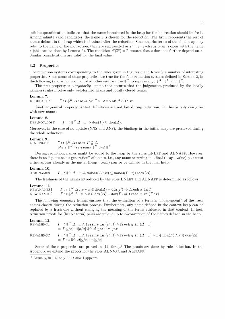
9
cofinite quantification indicates that the name introduced in the heap for the indirection should be fresh.Among infinite valid candidates, the name z is chosen for the reduction. The list z represents the rest ofnames defined in the heap which is obtained after the reduction. Since the rhs terms of this final heap mayrefer to the name of the indirection, they are represented as sz, i.e., each rhs term is open with the namez (this can be done by Lemma 6). The condition \y(sy) = s ensures that s does not further depend on z.Similar considerations are valid for the final value.
3.3 Properties
The reduction systems corresponding to the rules given in Figures 5 and 6 verify a number of interestingproperties. Since some of these properties are true for the four reduction systems defined in Section 2, inthe following (and when not indicated otherwise) we use ⇓K to represent ⇓, ⇓A, ⇓I , and ⇓N .
The first property is a regularity lemma that ensures that the judgements produced by the locallynameless rules involve only well-formed heaps and locally closed terms:
Lemma 7.regularity Γ : t ⇓K ∆ : w ⇒ ok Γ ∧ lc t ∧ ok ∆ ∧ lc w
Another general property is that definitions are not lost during reduction, i.e., heaps only can growwith new names:
Lemma 8.def not lost Γ : t ⇓K ∆ : w ⇒ dom(Γ ) ⊆ dom(∆).
Moreover, in the case of no update (NNS and ANS), the bindings in the initial heap are preserved duringthe whole reduction:
Lemma 9.no update Γ : t ⇓K ∆ : w⇒ Γ ⊆ ∆
where ⇓K represents ⇓N and ⇓A
During reduction, names might be added to the heap by the rules LNLet and ALNApp. However,there is no “spontaneous generation” of names, i.e., any name occurring in a final (heap : value) pair musteither appear already in the initial (heap : term) pair or be defined in the final heap:
Lemma 10.add names Γ : t ⇓K ∆ : w⇒ names(∆ : w) ⊆ names(Γ : t) ∪ dom(∆).
The freshness of the names introduced by the rules LNLet and ALNApp is determined as follows:
Lemma 11.new names1 Γ : t ⇓N ∆ : w ∧ x ∈ dom(∆)− dom(Γ )⇒ fresh x in Γnew names2 Γ : t ⇓A ∆ : w ∧ x ∈ dom(∆) − dom(Γ )⇒ fresh x in (Γ : t)
The following renaming lemma ensures that the evaluation of a term is “independent” of the freshnames chosen during the reduction process. Furthermore, any name defined in the context heap can bereplaced by a fresh one without changing the meaning of the terms evaluated in that context. In fact,reduction proofs for (heap : term) pairs are unique up to α-conversion of the names defined in the heap.
Lemma 12.renaming1 Γ : t ⇓K ∆ : w ∧ fresh y in (Γ : t) ∧ fresh y in (∆ : w)
⇒ Γ [y/x] : t[y/x] ⇓K ∆[y/x] : w[y/x]
renaming2 Γ : t ⇓K ∆ : w ∧ fresh y in (Γ : t) ∧ fresh y in (∆ : w) ∧ x /∈ dom(Γ ) ∧ x ∈ dom(∆)⇒ Γ : t ⇓K ∆[y/x] : w[y/x]
Some of these properties are proved in [14] for ⇓.3 The proofs are done by rule induction. In theAppendix we extend the proofs for the rules ALNVar and ALNApp.
3 Actually, in [14] only renaming1 appears.
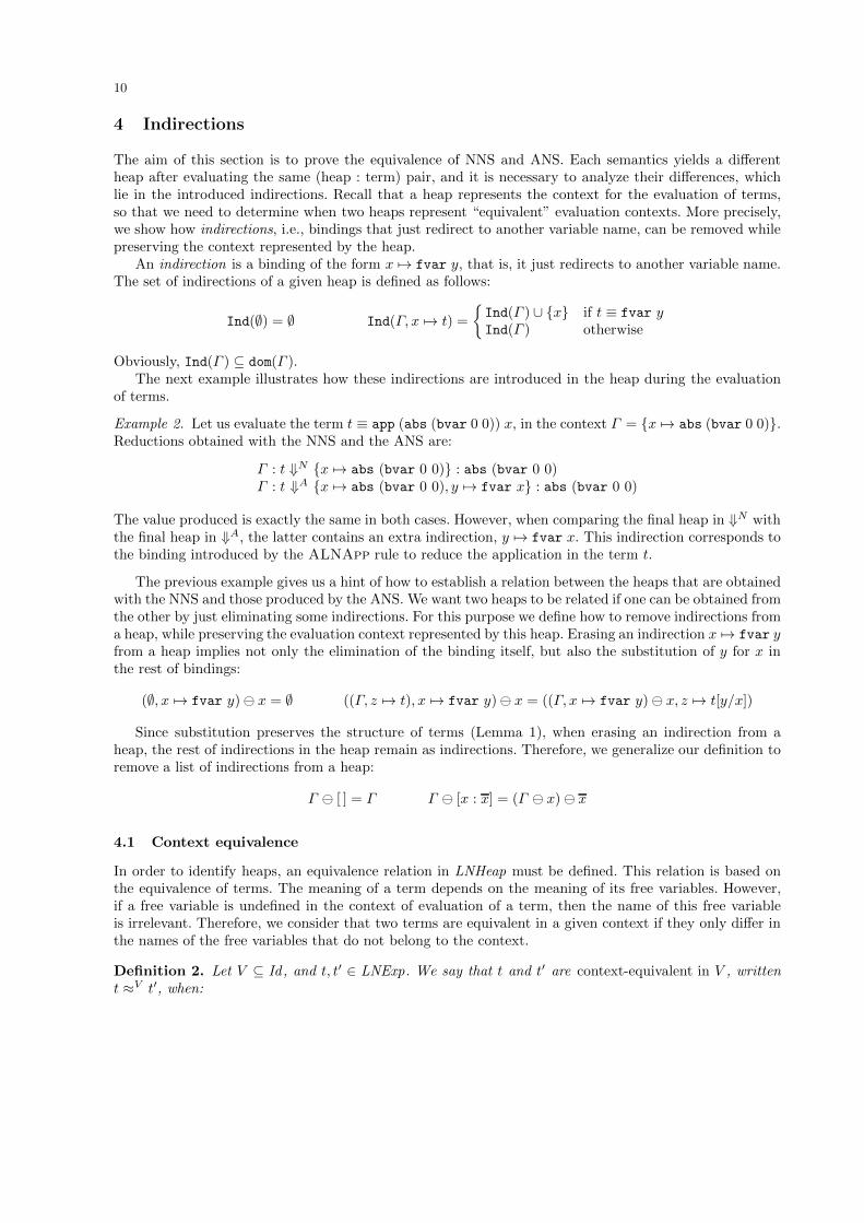
10
4 Indirections
The aim of this section is to prove the equivalence of NNS and ANS. Each semantics yields a differentheap after evaluating the same (heap : term) pair, and it is necessary to analyze their differences, whichlie in the introduced indirections. Recall that a heap represents the context for the evaluation of terms,so that we need to determine when two heaps represent “equivalent” evaluation contexts. More precisely,we show how indirections, i.e., bindings that just redirect to another variable name, can be removed whilepreserving the context represented by the heap.
An indirection is a binding of the form x 7→ fvar y, that is, it just redirects to another variable name.The set of indirections of a given heap is defined as follows:
Ind(∅) = ∅ Ind(Γ, x 7→ t) =
{Ind(Γ ) ∪ {x} if t ≡ fvar yInd(Γ ) otherwise
Obviously, Ind(Γ ) ⊆ dom(Γ ).The next example illustrates how these indirections are introduced in the heap during the evaluation
of terms.
Example 2. Let us evaluate the term t ≡ app (abs (bvar 0 0)) x, in the context Γ = {x 7→ abs (bvar 0 0)}.Reductions obtained with the NNS and the ANS are:
Γ : t ⇓N {x 7→ abs (bvar 0 0)} : abs (bvar 0 0)Γ : t ⇓A {x 7→ abs (bvar 0 0), y 7→ fvar x} : abs (bvar 0 0)
The value produced is exactly the same in both cases. However, when comparing the final heap in ⇓N withthe final heap in ⇓A, the latter contains an extra indirection, y 7→ fvar x. This indirection corresponds tothe binding introduced by the ALNApp rule to reduce the application in the term t.
The previous example gives us a hint of how to establish a relation between the heaps that are obtainedwith the NNS and those produced by the ANS. We want two heaps to be related if one can be obtained fromthe other by just eliminating some indirections. For this purpose we define how to remove indirections froma heap, while preserving the evaluation context represented by this heap. Erasing an indirection x 7→ fvar yfrom a heap implies not only the elimination of the binding itself, but also the substitution of y for x inthe rest of bindings:
(∅, x 7→ fvar y)⊖ x = ∅ ((Γ, z 7→ t), x 7→ fvar y)⊖ x = ((Γ, x 7→ fvar y)⊖ x, z 7→ t[y/x])
Since substitution preserves the structure of terms (Lemma 1), when erasing an indirection from aheap, the rest of indirections in the heap remain as indirections. Therefore, we generalize our definition toremove a list of indirections from a heap:
Γ ⊖ [ ] = Γ Γ ⊖ [x : x] = (Γ ⊖ x)⊖ x
4.1 Context equivalence
In order to identify heaps, an equivalence relation in LNHeap must be defined. This relation is based onthe equivalence of terms. The meaning of a term depends on the meaning of its free variables. However,if a free variable is undefined in the context of evaluation of a term, then the name of this free variableis irrelevant. Therefore, we consider that two terms are equivalent in a given context if they only differ inthe names of the free variables that do not belong to the context.
Definition 2. Let V ⊆ Id, and t, t′ ∈ LNExp. We say that t and t′ are context-equivalent in V , writtent ≈V t′, when:
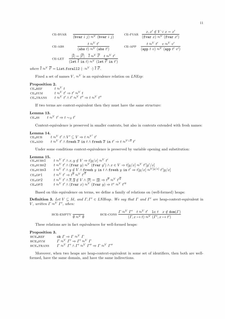
11
ce-bvar(bvar i j) ≈V (bvar i j)
ce-fvarx, x′ /∈ V ∨ x = x′
(fvar x) ≈V (fvar x′)
ce-abst ≈V t′
(abs t) ≈V (abs t′)ce-app
t ≈V t′ v ≈V v′
(app t v) ≈V (app t′ v′)
ce-let|t| = |t′| t ≈V t′ t ≈V t′
(let t in t) ≈V (let t′ in t′)
where t ≈V t′ = List.forall2 (· ≈V ·) t t′.
Fixed a set of names V , ≈V is an equivalence relation on LNExp:
Proposition 2.ce ref t ≈V tce sym t ≈V t′ ⇒ t′ ≈V tce trans t ≈V t′ ∧ t′ ≈V t′′ ⇒ t ≈V t′′
If two terms are context-equivalent then they must have the same structure:
Lemma 13.ce ss t ≈V t′ ⇒ t ∼S t′
Context-equivalence is preserved in smaller contexts, but also in contexts extended with fresh names:
Lemma 14.ce sub t ≈V t′ ∧ V ′ ⊆ V ⇒ t ≈V ′
t′
ce add t ≈V t′ ∧ fresh x in t ∧ fresh x in t′ ⇒ t ≈V ∪x t′
Under some conditions context-equivalence is preserved by variable opening and substitution:
Lemma 15.ce subs1 t ≈V t′ ∧ x, y /∈ V ⇒ t[y/x] ≈V t′
ce subs2 t ≈V t′ ∧ (fvar y) ≈V (fvar y′) ∧ x ∈ V ⇒ t[y/x] ≈V t′[y′/x]
ce subs3 t ≈V t′ ∧ y /∈ V ∧ fresh y in t ∧ fresh y in t′ ⇒ t[y/x] ≈V [y/x] t′[y/x]
ce op1 t ≈V t′ ⇒ tx ≈V t′x
ce op2 t ≈V t′ ∧ x, y /∈ V ∧ |x| = |y| ⇒ tx ≈V t′y
ce op3 t ≈V t′ ∧ (fvar x) ≈V (fvar y)⇒ tx ≈V t′y
Based on this equivalence on terms, we define a family of relations on (well-formed) heaps:
Definition 3. Let V ⊆ Id, and Γ, Γ ′ ∈ LNHeap. We say that Γ and Γ ′ are heap-context-equivalent inV , written Γ ≈V Γ ′, when:
hce-empty ∅ ≈V ∅ hce-consΓ ≈V Γ ′ t ≈V t′ lc t x /∈ dom(Γ )
(Γ, x 7→ t) ≈V (Γ ′, x 7→ t′)
These relations are in fact equivalences for well-formed heaps:
Proposition 3.hce ref ok Γ ⇒ Γ ≈V Γhce sym Γ ≈V Γ ′ ⇒ Γ ′ ≈V Γhce trans Γ ≈V Γ ′ ∧ Γ ′ ≈V Γ ′′ ⇒ Γ ≈V Γ ′′
Moreover, when two heaps are heap-context-equivalent in some set of identifiers, then both are well-formed, have the same domain, and have the same indirections.

12
Lemma 16.hce dom Γ ≈V Γ ′ ⇒ dom(Γ ) = dom(Γ ′)hce ind Γ ≈V Γ ′ ⇒ Ind(Γ ) = Ind(Γ ′)hce ok Γ ≈V Γ ′ ⇒ ok Γ ∧ ok Γ ′
There is an alternative characterization for heap-context-equivalence which expresses that two heapsare context-equivalent whenever they have the same domain and each pair of corresponding bound termsis context-equivalent.
Lemma 17.hce alt Γ ≈V Γ ′ ⇔ ok Γ ∧ ok Γ ′ ∧ dom(Γ ) = dom(Γ ′) ∧ (x 7→ t ∈ Γ ∧ x 7→ t′ ∈ Γ ′ ⇒ t ≈V t′)
Next results guarantee uniqueness up to permutations of sequence of indirections that makes two heapsbe equivalent. The order in which two indirections are removed from a heap can be exchanged and theproduced heaps are context-equivalent.
Lemma 18.hce swap ok Γ ∧ x, y ∈ Ind(Γ ) ∧ x 6= y ⇒ Γ ⊖ [x, y] ≈V−{x,y} Γ ⊖ [y, x]
Considering context-equivalence on heaps, we are particularly interested in the case where the contextcoincides with the domain of the heaps:
Definition 4. Let Γ, Γ ′ ∈ LNHeap. We say that Γ and Γ ′ are heap-equivalent, written Γ ≈ Γ ′, if theyare heap-context-equivalent in dom(Γ ):
heΓ ≈dom(Γ ) Γ ′
Γ ≈ Γ ′
Lemma 18 can be generalized to a list of indirections and its permutations.
Lemma 19.he perm ok Γ ∧ x, y ⊆ Ind(Γ )⇒ (Γ ⊖ x ≈ Γ ⊖ y ⇔ y ∈ S(x))
where S(x) denotes the set of all permutations of x.
4.2 Indirection Relation
Coming back to the idea, shown in Example 2, that a heap can be obtained from another by just removingsome indirections, we define the following relation on heaps:
Definition 5. Let Γ, Γ ′ ∈ LNHeap. Γ is indirection-related to Γ ′, written Γ %I Γ ′, when:
ir-heΓ ≈ Γ ′
Γ %I Γ ′ ir-irok Γ Γ ⊖ x %I Γ ′ x ∈ Ind(Γ )
Γ %I Γ ′
There is an alternative characterization for the relation %I which expresses that a heap is indirection-related to another whenever the later can be obtained from the former by erasing a sequence of indirections.
Proposition 4.ir alt Γ %I Γ ′ ⇔ ok Γ ∧ ∃ x ⊆ Ind(Γ ) . Γ ⊖ x ≈ Γ ′
Furthermore, this sequence of indirections is unique up to permutations (by Lemma 19), and it corre-sponds to the difference between the domains of the related heaps:
Corollary 1.ir dom dom Γ %I Γ ′ ⇒ Γ ⊖ (dom(Γ )− dom(Γ ′)) ≈ Γ ′ 4
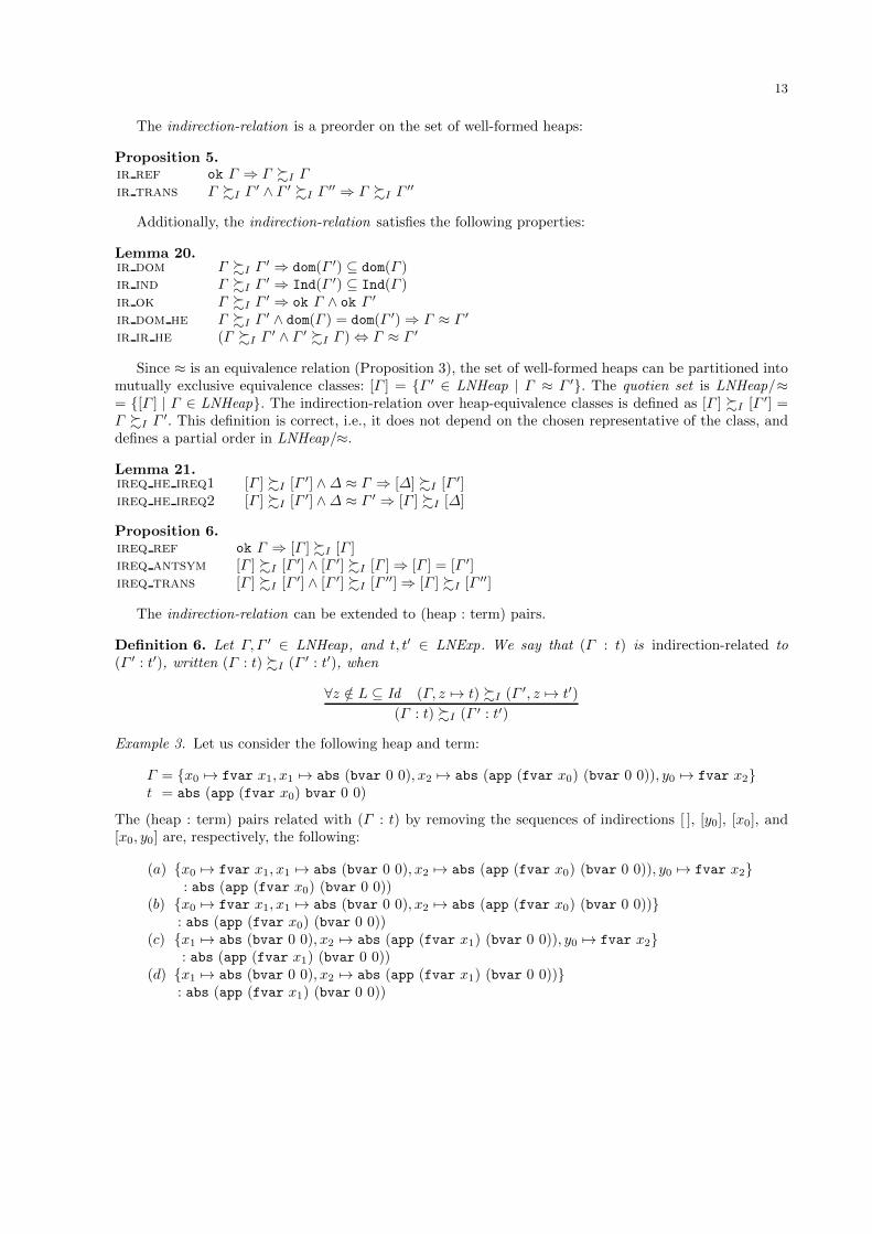
13
The indirection-relation is a preorder on the set of well-formed heaps:
Proposition 5.ir ref ok Γ ⇒ Γ %I Γir trans Γ %I Γ ′ ∧ Γ ′ %I Γ ′′ ⇒ Γ %I Γ ′′
Additionally, the indirection-relation satisfies the following properties:
Lemma 20.ir dom Γ %I Γ ′ ⇒ dom(Γ ′) ⊆ dom(Γ )ir ind Γ %I Γ ′ ⇒ Ind(Γ ′) ⊆ Ind(Γ )ir ok Γ %I Γ ′ ⇒ ok Γ ∧ ok Γ ′
ir dom he Γ %I Γ ′ ∧ dom(Γ ) = dom(Γ ′)⇒ Γ ≈ Γ ′
ir ir he (Γ %I Γ ′ ∧ Γ ′ %I Γ )⇔ Γ ≈ Γ ′
Since ≈ is an equivalence relation (Proposition 3), the set of well-formed heaps can be partitioned intomutually exclusive equivalence classes: [Γ ] = {Γ ′ ∈ LNHeap | Γ ≈ Γ ′}. The quotien set is LNHeap/≈= {[Γ ] | Γ ∈ LNHeap}. The indirection-relation over heap-equivalence classes is defined as [Γ ] %I [Γ ′] =Γ %I Γ ′. This definition is correct, i.e., it does not depend on the chosen representative of the class, anddefines a partial order in LNHeap/≈.
Lemma 21.ireq he ireq1 [Γ ] %I [Γ ′] ∧∆ ≈ Γ ⇒ [∆] %I [Γ ′]ireq he ireq2 [Γ ] %I [Γ ′] ∧∆ ≈ Γ ′ ⇒ [Γ ] %I [∆]
Proposition 6.ireq ref ok Γ ⇒ [Γ ] %I [Γ ]ireq antsym [Γ ] %I [Γ ′] ∧ [Γ ′] %I [Γ ]⇒ [Γ ] = [Γ ′]ireq trans [Γ ] %I [Γ ′] ∧ [Γ ′] %I [Γ ′′]⇒ [Γ ] %I [Γ ′′]
The indirection-relation can be extended to (heap : term) pairs.
Definition 6. Let Γ, Γ ′ ∈ LNHeap, and t, t′ ∈ LNExp. We say that (Γ : t) is indirection-related to(Γ ′ : t′), written (Γ : t) %I (Γ ′ : t′), when
∀z /∈ L ⊆ Id (Γ, z 7→ t) %I (Γ ′, z 7→ t′)
(Γ : t) %I (Γ ′ : t′)
Example 3. Let us consider the following heap and term:
Γ = {x0 7→ fvar x1, x1 7→ abs (bvar 0 0), x2 7→ abs (app (fvar x0) (bvar 0 0)), y0 7→ fvar x2}t = abs (app (fvar x0) bvar 0 0)
The (heap : term) pairs related with (Γ : t) by removing the sequences of indirections [ ], [y0], [x0], and[x0, y0] are, respectively, the following:
(a) {x0 7→ fvar x1, x1 7→ abs (bvar 0 0), x2 7→ abs (app (fvar x0) (bvar 0 0)), y0 7→ fvar x2}: abs (app (fvar x0) (bvar 0 0))
(b) {x0 7→ fvar x1, x1 7→ abs (bvar 0 0), x2 7→ abs (app (fvar x0) (bvar 0 0))}: abs (app (fvar x0) (bvar 0 0))
(c) {x1 7→ abs (bvar 0 0), x2 7→ abs (app (fvar x1) (bvar 0 0)), y0 7→ fvar x2}: abs (app (fvar x1) (bvar 0 0))
(d) {x1 7→ abs (bvar 0 0), x2 7→ abs (app (fvar x1) (bvar 0 0))}: abs (app (fvar x1) (bvar 0 0))
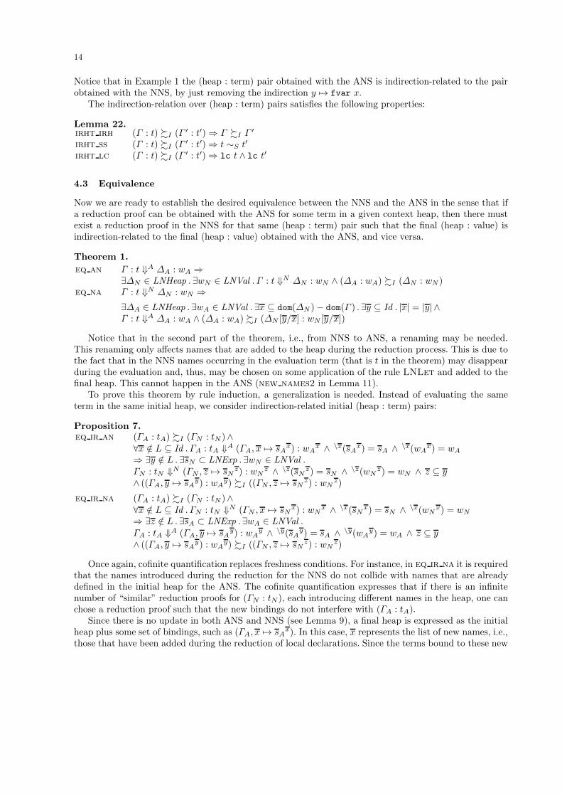
14
Notice that in Example 1 the (heap : term) pair obtained with the ANS is indirection-related to the pairobtained with the NNS, by just removing the indirection y 7→ fvar x.
The indirection-relation over (heap : term) pairs satisfies the following properties:
Lemma 22.irht irh (Γ : t) %I (Γ ′ : t′)⇒ Γ %I Γ ′
irht ss (Γ : t) %I (Γ ′ : t′)⇒ t ∼S t′
irht lc (Γ : t) %I (Γ ′ : t′)⇒ lc t ∧ lc t′
4.3 Equivalence
Now we are ready to establish the desired equivalence between the NNS and the ANS in the sense that ifa reduction proof can be obtained with the ANS for some term in a given context heap, then there mustexist a reduction proof in the NNS for that same (heap : term) pair such that the final (heap : value) isindirection-related to the final (heap : value) obtained with the ANS, and vice versa.
Theorem 1.
eq an Γ : t ⇓A ∆A : wA ⇒∃∆N ∈ LNHeap . ∃wN ∈ LNVal . Γ : t ⇓N ∆N : wN ∧ (∆A : wA) %I (∆N : wN )
eq na Γ : t ⇓N ∆N : wN ⇒∃∆A ∈ LNHeap . ∃wA ∈ LNVal . ∃x ⊆ dom(∆N )− dom(Γ ) . ∃y ⊆ Id . |x| = |y| ∧Γ : t ⇓A ∆A : wA ∧ (∆A : wA) %I (∆N [y/x] : wN [y/x])
Notice that in the second part of the theorem, i.e., from NNS to ANS, a renaming may be needed.This renaming only affects names that are added to the heap during the reduction process. This is due tothe fact that in the NNS names occurring in the evaluation term (that is t in the theorem) may disappearduring the evaluation and, thus, may be chosen on some application of the rule LNLet and added to thefinal heap. This cannot happen in the ANS (new names2 in Lemma 11).
To prove this theorem by rule induction, a generalization is needed. Instead of evaluating the sameterm in the same initial heap, we consider indirection-related initial (heap : term) pairs:
Proposition 7.eq ir an (ΓA : tA) %I (ΓN : tN )∧
∀x /∈ L ⊆ Id . ΓA : tA ⇓A (ΓA, x 7→ sAx) : wA
x ∧ \x(sAx) = sA ∧ \x(wA
x) = wA
⇒ ∃y /∈ L . ∃sN ⊂ LNExp . ∃wN ∈ LNVal .ΓN : tN ⇓N (ΓN , z 7→ sN
z) : wNz ∧ \z(sNz) = sN ∧ \z(wN
z) = wN ∧ z ⊆ y∧ ((ΓA, y 7→ sA
y) : wAy) %I ((ΓN , z 7→ sN
z) : wNz)
eq ir na (ΓA : tA) %I (ΓN : tN )∧∀x /∈ L ⊆ Id . ΓN : tN ⇓N (ΓN , x 7→ sN
x) : wNx ∧ \x(sN
x) = sN ∧ \x(wNx) = wN
⇒ ∃z /∈ L . ∃sA ⊂ LNExp . ∃wA ∈ LNVal .
ΓA : tA ⇓A (ΓA, y 7→ sAy) : wA
y ∧ \y(sAy) = sA ∧ \y(wAy) = wA ∧ z ⊆ y
∧ ((ΓA, y 7→ sAy) : wA
y) %I ((ΓN , z 7→ sNz) : wN
z)
Once again, cofinite quantification replaces freshness conditions. For instance, in eq ir na it is requiredthat the names introduced during the reduction for the NNS do not collide with names that are alreadydefined in the initial heap for the ANS. The cofinite quantification expresses that if there is an infinitenumber of “similar” reduction proofs for (ΓN : tN ), each introducing different names in the heap, one canchose a reduction proof such that the new bindings do not interfere with (ΓA : tA).
Since there is no update in both ANS and NNS (see Lemma 9), a final heap is expressed as the initialheap plus some set of bindings, such as (ΓA, x 7→ sA
x). In this case, x represents the list of new names, i.e.,those that have been added during the reduction of local declarations. Since the terms bound to these new
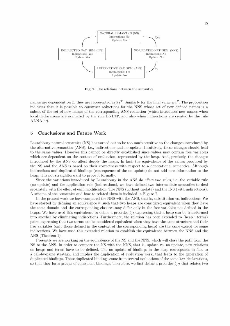
15
NATURAL SEMANTICS (NS)Indirections: NoUpdate: Yes
INDIRECTED NAT. SEM. (INS)Indirections: YesUpdate: Yes
NO-UPDATED NAT. SEM. (NNS)Indirections: NoUpdate: No
ALTERNATIVE NAT. SEM. (ANS)Indirections: Yes
Update: No
%I
%GU
Fig. 7. The relations between the semantics
names are dependent on x, they are represented as sAx. Similarly for the final value wA
x. The propositionindicates that it is possible to construct reductions for the NNS whose set of new defined names is asubset of the set of new names of the corresponding ANS reduction (which introduces new names whenlocal declarations are evaluated by the rule LNLet, and also when indirections are created by the ruleALNApp).
5 Conclusions and Future Work
Launchbury natural semantics (NS) has turned out to be too much sensitive to the changes introduced bythe alternative semantics (ANS), i.e., indirections and no-update. Intuitively, these changes should leadto the same values. However this cannot be directly established since values may contain free variableswhich are dependent on the context of evaluation, represented by the heap. And, precisely, the changesintroduced by the ANS do affect deeply the heaps. In fact, the equivalence of the values produced bythe NS and the ANS is based on their correctness with respect to a denotational semantics. Althoughindirections and duplicated bindings (consequence of the no-update) do not add new information to theheap, it is not straightforward to prove it formally.
Since the variations introduced by Launchbury in the ANS do affect two rules, i.e. the variable rule(no update) and the application rule (indirections), we have defined two intermediate semantics to dealseparately with the effect of each modification: The NNS (without update) and the INS (with indirections).A schema of the semantics and how to related them is included in Figure 7.
In the present work we have compared the NNS with the ANS, that is, substitution vs. indirections. Wehave started by defining an equivalence ≈ such that two heaps are considered equivalent when they havethe same domain and the corresponding closures may differ only in the free variables not defined in theheaps. We have used this equivalence to define a preorder %I expressing that a heap can be transformedinto another by eliminating indirections. Furthermore, the relation has been extended to (heap : terms)pairs, expressing that two terms can be considered equivalent when they have the same structure and theirfree variables (only those defined in the context of the corresponding heap) are the same except for someindirections. We have used this extended relation to establish the equivalence between the NNS and theANS (Theorem 1).
Presently we are working on the equivalence of the NS and the NNS, which will close the path from theNS to the ANS. In order to compare the NS with the NNS, that is, update vs. no update, new relationson heaps and terms have to be defined. The no update of bindings in the heap corresponds in fact toa call-by-name strategy, and implies the duplication of evaluation work, that leads to the generation ofduplicated bindings. These duplicated bindings come from several evaluations of the same let-declarations,so that they form groups of equivalent bindings. Therefore, we first define a preorder %G that relates two

16
heaps whenever the first can be transformed into the second by eliminating duplicated groups of bindings.Afterwards, we define a relation ∼U that establishes when a heap is an updated version of another heap.Finally, both relations must be combined to obtain the group-update relation %GU , which extended for(heap : terms) will allow us to formulate an equivalence theorem for the NS and the NNS, similar toTheorem 1.
Although the relations %I and %GU are sufficient for proving the equivalence of the NS and the ANS,it would be interesting to complete the picture by comparing the NS with the INS, and then the INS withthe AN. For the first step, we have to define a preorder similar to %I , but taking into account that extraindirections may now be updated, thus leading to “redundant” bindings. For the second step, some versionof the group-update relation is needed. Dashed lines indicate this future work.
We have used a locally nameless representation to avoid problems with α-equivalence, while keepinga readable formalization of the syntax and semantics. This representation allow us to treat with heapsin a convenient and easy way, avoiding the problems that arise when using the de Bruijn notation. Wehave also introduced cofinite quantification (in the style of [1]) in the evaluation rules that introduce freshnames, namely the rule for local declarations (LNLet) and for the alternative application (ALNApp).Moreover, this representation is more amenable to formalization in proof assistants. In fact we have startedto implement the semantic rules given in Section 3.2 using Coq [4], with the intention of obtaining a formalchecking of our proofs. At this point we should mention the work of Joachim Breitner who is working onthe formalization of the correctness and adequacy of Launchbury’s semantics by using Isabelle [10]. So farhe has been able to mechanically verify the correctness of the operational semantics with respect to thedenotational one [5].
6 Acknowledgments
This work is partially supported by the projects: TIN2012-39391-C04-04 and S2009/TIC-1465.
References
1. B. E. Aydemir, A. Chargueraud, B. C. Pierce, R. Pollack, and S. Weirich. Engineering formal metatheory.In Proceedings of ACM SIGPLAN-SIGACT Symposium on Principles of Programming Languages (POPL’08),pages 3–15. ACM Press, 2008.
2. C. Baker-Finch, D. King, and P. W. Trinder. An operational semantics for parallel lazy evaluation. In ACMSIGPLAN International Conference on Functional Programming (ICFP’00), pages 162–173. ACM Press, 2000.
3. H. P. Barendregt. The Lambda Calculus: Its Syntax and Semantics, volume 103 of Studies in Logic and theFoundations of Mathematics. North-Holland, 1984.
4. Y. Bertot. Coq in a hurry. CoRR, abs/cs/0603118, 2006.5. J. Breitner. The correctness of Launchbury’s natural semantics for lazy evaluation. Archive of formal proofs,
http://afp.sf.net/entries/Launchbury, 2013. Formal proof development.6. A. Chargueraud. The locally nameless representation. Journal of Automated Reasoning, 49(3):363–408, 2012.7. N. G. de Bruijn. Lambda calculus notation with nameless dummies, a tool for automatic formula manipulation,
with application to the Church-Rosser theorem. Indagationes Mathematicae, 75(5):381–392, 1972.8. J. Launchbury. A natural semantics for lazy evaluation. In Proceedings of ACM SIGPLAN-SIGACT Symposium
on Principles of Programming Languages (POPL’93), pages 144–154. ACM Press, 1993.9. K. Nakata and M. Hasegawa. Small-step and big-step semantics for call-by-need. Journal of Functional
Programming, 19(6):699–722, 2009.10. T. Nipkow, L. C. Paulson, and M. Wenzel. Isabelle/HOL — A Proof Assistant for Higher-Order Logic, volume
2283 of LNCS. Springer, 2002. http://isabelle.in.tum.de.11. L. Sanchez-Gil, M. Hidalgo-Herrero, and Y. Ortega-Mallen. Call-by-need, call-by-name, and natural semantics.
Technical Report UU-CS-2010-020, Departament of Information and Computing Sciences, Utrech University,2010.
12. L. Sanchez-Gil, M. Hidalgo-Herrero, and Y. Ortega-Mallen. Trends in Functional Programming, volume 10,chapter An Operational Semantics for Distributed Lazy Evaluation, pages 65–80. Intellect, 2010.
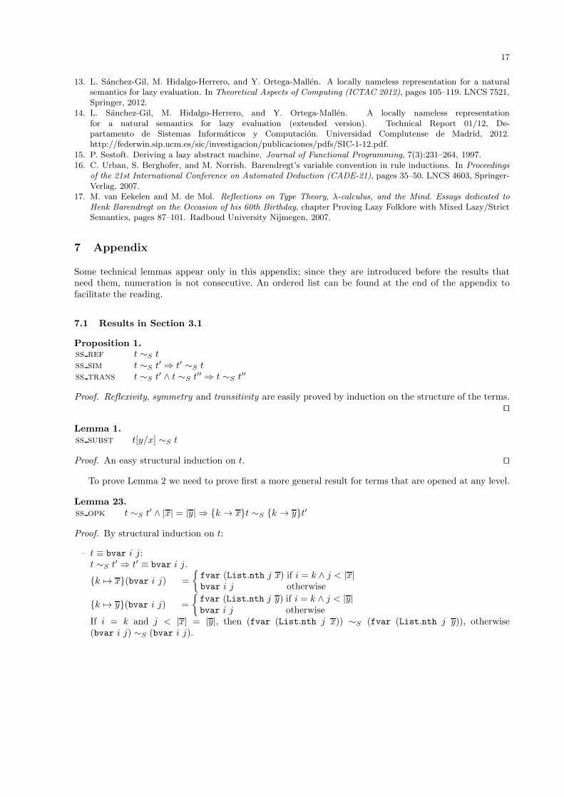
17
13. L. Sanchez-Gil, M. Hidalgo-Herrero, and Y. Ortega-Mallen. A locally nameless representation for a naturalsemantics for lazy evaluation. In Theoretical Aspects of Computing (ICTAC 2012), pages 105–119. LNCS 7521,Springer, 2012.
14. L. Sanchez-Gil, M. Hidalgo-Herrero, and Y. Ortega-Mallen. A locally nameless representationfor a natural semantics for lazy evaluation (extended version). Technical Report 01/12, De-partamento de Sistemas Informaticos y Computacion. Universidad Complutense de Madrid, 2012.http://federwin.sip.ucm.es/sic/investigacion/publicaciones/pdfs/SIC-1-12.pdf.
15. P. Sestoft. Deriving a lazy abstract machine. Journal of Functional Programming, 7(3):231–264, 1997.16. C. Urban, S. Berghofer, and M. Norrish. Barendregt’s variable convention in rule inductions. In Proceedings
of the 21st International Conference on Automated Deduction (CADE-21), pages 35–50. LNCS 4603, Springer-Verlag, 2007.
17. M. van Eekelen and M. de Mol. Reflections on Type Theory, λ-calculus, and the Mind. Essays dedicated toHenk Barendregt on the Occasion of his 60th Birthday, chapter Proving Lazy Folklore with Mixed Lazy/StrictSemantics, pages 87–101. Radboud University Nijmegen, 2007.
7 Appendix
Some technical lemmas appear only in this appendix; since they are introduced before the results thatneed them, numeration is not consecutive. An ordered list can be found at the end of the appendix tofacilitate the reading.
7.1 Results in Section 3.1
Proposition 1.ss ref t ∼S tss sim t ∼S t′ ⇒ t′ ∼S tss trans t ∼S t′ ∧ t ∼S t′′ ⇒ t ∼S t′′
Proof. Reflexivity, symmetry and transitivity are easily proved by induction on the structure of the terms.⊓⊔
Lemma 1.ss subst t[y/x] ∼S t
Proof. An easy structural induction on t. ⊓⊔
To prove Lemma 2 we need to prove first a more general result for terms that are opened at any level.
Lemma 23.ss opk t ∼S t′ ∧ |x| = |y| ⇒ {k → x}t ∼S {k→ y}t′
Proof. By structural induction on t:
– t ≡ bvar i j:t ∼S t′ ⇒ t′ ≡ bvar i j.
{k 7→ x}(bvar i j) =
{fvar (List.nth j x) if i = k ∧ j < |x|bvar i j otherwise
{k 7→ y}(bvar i j) =
{fvar (List.nth j y) if i = k ∧ j < |y|bvar i j otherwise
If i = k and j < |x| = |y|, then (fvar (List.nth j x)) ∼S (fvar (List.nth j y)), otherwise(bvar i j) ∼S (bvar i j).
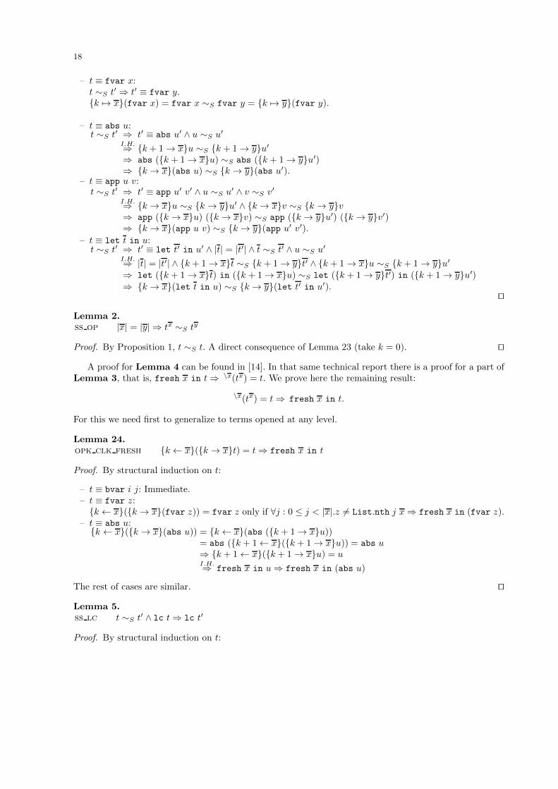
18
– t ≡ fvar x:t ∼S t′ ⇒ t′ ≡ fvar y.{k 7→ x}(fvar x) = fvar x ∼S fvar y = {k 7→ y}(fvar y).
– t ≡ abs u:t ∼S t′ ⇒ t′ ≡ abs u′ ∧ u ∼S u′
I.H.⇒ {k + 1→ x}u ∼S {k + 1→ y}u′
⇒ abs ({k + 1→ x}u) ∼S abs ({k + 1→ y}u′)⇒ {k→ x}(abs u) ∼S {k → y}(abs u′).
– t ≡ app u v:t ∼S t′ ⇒ t′ ≡ app u′ v′ ∧ u ∼S u′ ∧ v ∼S v′
I.H.⇒ {k→ x}u ∼S {k → y}u′ ∧ {k→ x}v ∼S {k → y}v⇒ app ({k → x}u) ({k → x}v) ∼S app ({k→ y}u′) ({k → y}v′)⇒ {k→ x}(app u v) ∼S {k → y}(app u′ v′).
– t ≡ let t in u:t ∼S t′ ⇒ t′ ≡ let t′ in u′ ∧ |t| = |t′| ∧ t ∼S t′ ∧ u ∼S u′
I.H.⇒ |t| = |t′| ∧ {k + 1→ x}t ∼S {k + 1→ y}t′ ∧ {k + 1→ x}u ∼S {k + 1→ y}u′
⇒ let ({k + 1→ x}t) in ({k + 1→ x}u) ∼S let ({k + 1→ y}t′) in ({k + 1→ y}u′)⇒ {k→ x}(let t in u) ∼S {k→ y}(let t′ in u′).
⊓⊔
Lemma 2.ss op |x| = |y| ⇒ tx ∼S ty
Proof. By Proposition 1, t ∼S t. A direct consequence of Lemma 23 (take k = 0). ⊓⊔
A proof for Lemma 4 can be found in [14]. In that same technical report there is a proof for a part ofLemma 3, that is, fresh x in t⇒ \x(tx) = t. We prove here the remaining result:
\x(tx) = t⇒ fresh x in t.
For this we need first to generalize to terms opened at any level.
Lemma 24.opk clk fresh {k← x}({k→ x}t) = t⇒ fresh x in t
Proof. By structural induction on t:
– t ≡ bvar i j: Immediate.– t ≡ fvar z:{k← x}({k→ x}(fvar z)) = fvar z only if ∀j : 0 ≤ j < |x|.z 6= List.nth j x⇒ fresh x in (fvar z).
– t ≡ abs u:{k ← x}({k → x}(abs u)) = {k ← x}(abs ({k + 1→ x}u))
= abs ({k + 1← x}({k + 1→ x}u)) = abs u⇒ {k + 1← x}({k + 1→ x}u) = uI.H.⇒ fresh x in u⇒ fresh x in (abs u)
The rest of cases are similar. ⊓⊔
Lemma 5.ss lc t ∼S t′ ∧ lc t⇒ lc t′
Proof. By structural induction on t:
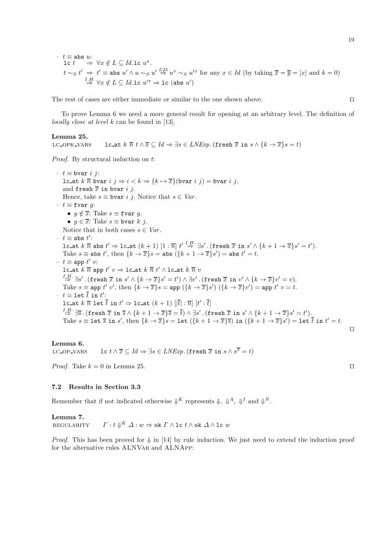
19
– t ≡ abs u:lc t ⇒ ∀x /∈ L ⊆ Id .lc ux.
t ∼S t′ ⇒ t′ ≡ abs u′ ∧ u ∼S u′ L23⇒ ux ∼S u′x for any x ∈ Id (by taking x = y = [x] and k = 0)I.H.⇒ ∀x /∈ L ⊆ Id .lc u′x ⇒ lc (abs u′)
The rest of cases are either immediate or similar to the one shown above. ⊓⊔
To prove Lemma 6 we need a more general result for opening at an arbitrary level. The definition oflocally close at level k can be found in [13].
Lemma 25.lc opk vars lc at k n t ∧ x ⊆ Id ⇒ ∃s ∈ LNExp. (fresh x in s ∧ {k→ x}s = t)
Proof. By structural induction on t:
– t ≡ bvar i j:lc at k n bvar i j ⇒ i < k ⇒ {k 7→ x}(bvar i j) = bvar i j,and fresh x in bvar i j.Hence, take s ≡ bvar i j. Notice that s ∈ Var .
– t ≡ fvar y:
• y /∈ x: Take s ≡ fvar y.• y ∈ x: Take s ≡ bvar k j.
Notice that in both cases s ∈ Var .– t ≡ abs t′:lc at k n abs t′ ⇒ lc at (k + 1) [1 : n] t′
I.H.⇒ ∃s′ . (fresh x in s′ ∧ {k + 1→ x}s′ = t′).Take s ≡ abs t′, then {k→ x}s = abs ({k + 1→ x}s′) = abs t′ = t.
– t ≡ app t′ v:lc at k n app t′ v ⇒ lc at k n t′ ∧ lc at k n vI.H.⇒ ∃s′ . (fresh x in s′ ∧ {k→ x}s′ = t′) ∧ ∃v′ . (fresh x in v′ ∧ {k→ x}v′ = v).Take s ≡ app t′ v′, then {k→ x}s = app ({k → x}s′) ({k → x}v′) = app t′ v = t.
– t ≡ let t in t′:lc at k n let t in t′ ⇒ lc at (k + 1) [|t| : n] [t′ : t]I.H.⇒ ∃s . (fresh x in s ∧ {k + 1→ x}s = t) ∧ ∃s′ . (fresh x in s′ ∧ {k + 1→ x}s′ = t′).Take s ≡ let s in s′, then {k→ x}s = let ({k + 1→ x}s) in ({k + 1→ x}s′) = let t in t′ = t.
⊓⊔
Lemma 6.lc op vars lc t ∧ x ⊆ Id ⇒ ∃s ∈ LNExp. (fresh x in s ∧ sx = t)
Proof. Take k = 0 in Lemma 25. ⊓⊔
7.2 Results in Section 3.3
Remember that if not indicated otherwise ⇓K represents ⇓, ⇓A, ⇓I and ⇓N .
Lemma 7.regularity Γ : t ⇓K ∆ : w ⇒ ok Γ ∧ lc t ∧ ok ∆ ∧ lc w
Proof. This has been proved for ⇓ in [14] by rule induction. We just need to extend the induction prooffor the alternative rules ALNVar and ALNApp:
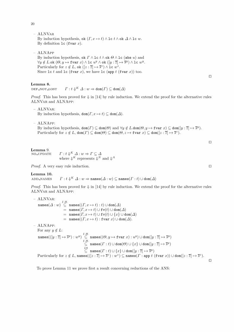
20
– ALNVarBy induction hypothesis, ok (Γ, x 7→ t) ∧ lc t ∧ ok ∆ ∧ lc w.By definition lc (fvar x).
– ALNAppBy induction hypothesis, ok Γ ∧ lc t ∧ ok Θ ∧ lc (abs u) and∀y /∈ L.ok (Θ, y 7→ fvar x) ∧ lc uy ∧ ok ([y : z] 7→ sy) ∧ lc wy .Particularly for z /∈ L, ok ([z : z] 7→ sz) ∧ lc wz .Since lc t and lc (fvar x), we have lc (app t (fvar x)) too.
⊓⊔
Lemma 8.def not lost Γ : t ⇓K ∆ : w ⇒ dom(Γ ) ⊆ dom(∆)
Proof. This has been proved for ⇓ in [14] by rule induction. We extend the proof for the alternative rulesALNVar and ALNApp:
– ALNVar:By induction hypothesis, dom(Γ, x 7→ t) ⊆ dom(∆).
– ALNApp:By induction hypothesis, dom(Γ ) ⊆ dom(Θ) and ∀y /∈ L.dom(Θ, y 7→ fvar x) ⊆ dom([y : z] 7→ sy).Particularly for z /∈ L, dom(Γ ) ⊆ dom(Θ) ⊆ dom(Θ, z 7→ fvar x) ⊆ dom([z : z] 7→ sz).
⊓⊔
Lemma 9.no update Γ : t ⇓K ∆ : w ⇒ Γ ⊆ ∆
where ⇓K represents ⇓N and ⇓A
Proof. A very easy rule induction. ⊓⊔
Lemma 10.add names Γ : t ⇓K ∆ : w ⇒ names(∆ : w) ⊆ names(Γ : t) ∪ dom(∆)
Proof. This has been proved for ⇓ in [14] by rule induction. We extend the proof for the alternative rulesALNVar and ALNApp:
– ALNVar:
names(∆ : w)I.H.⊆ names((Γ, x 7→ t) : t) ∪ dom(∆)= names(Γ, x 7→ t) ∪ fv(t) ∪ dom(∆)= names(Γ, x 7→ t) ∪ fv(t) ∪ {x} ∪ dom(∆)= names((Γ, x 7→ t) : fvar x) ∪ dom(∆).
– ALNApp:For any y /∈ L:
names(([y : z] 7→ sy) : wy)I.H.⊆ names((Θ, y 7→ fvar x) : uy) ∪ dom([y : z] 7→ sy)
I.H.⊆ names(Γ : t) ∪ dom(Θ) ∪ {x} ∪ dom([y : z] 7→ sy)L8⊆ names(Γ : t) ∪ {x} ∪ dom([y : z] 7→ sy)
Particularly for z /∈ L, names(([z : z] 7→ sz) : wz) ⊆ names(Γ : app t (fvar x)) ∪ dom([z : z] 7→ sz).⊓⊔
To prove Lemma 11 we prove first a result concerning reductions of the ANS:
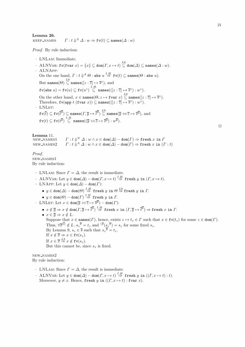
21
Lemma 26.keep names Γ : t ⇓A ∆ : w ⇒ fv(t) ⊆ names(∆ : w)
Proof. By rule induction:
– LNLam: Immediate.
– ALNVar: fv(fvar x) = {x} ⊆ dom(Γ, x 7→ t)L8⊆ dom(∆) ⊆ names(∆ : w).
– ALNApp:On the one hand, Γ : t ⇓A Θ : abs u
I.H.⇒ fv(t) ⊆ names(Θ : abs u).
But names(Θ)L9⊆ names([z : z] 7→ sz), and
fv(abs u) = fv(u) ⊆ fv(uz)I.H.⊆ names(([z : z] 7→ sz) : wz).
On the other hand, x ∈ names(Θ, z 7→ fvar x)L9⊆ names([z : z] 7→ sz).
Therefore, fv(app t (fvar x)) ⊆ names(([z : z] 7→ sz) : wz).
– LNLet:
fv(t) ⊆ fv(ty) ⊆ names(Γ, y 7→ t
y)L9⊆ names(y ++z 7→ sy), and
fv(t) ⊆ fv(ty)I.H.⊆ names((y ++z 7→ sy) : wy).
⊓⊔
Lemma 11.new names1 Γ : t ⇓N ∆ : w ∧ x ∈ dom(∆)− dom(Γ )⇒ fresh x in Γnew names2 Γ : t ⇓A ∆ : w ∧ x ∈ dom(∆)− dom(Γ )⇒ fresh x in (Γ : t)
Proof.new names1By rule induction:
– LNLam: Since Γ = ∆, the result is immediate.
– ALNVar: Let y ∈ dom(∆)− dom(Γ, x 7→ t)I.H.⇒ fresh y in (Γ, x 7→ t).
– LNApp: Let y ∈ dom(∆)− dom(Γ ):
• y ∈ dom(∆)− dom(Θ)I.H.⇒ fresh y in Θ
L9⇒ fresh y in Γ.
• y ∈ dom(Θ)− dom(Γ )I.H.⇒ fresh y in Γ.
– LNLet: Let x ∈ dom(y ++z 7→ sy)− dom(Γ ):
• x /∈ y ⇒ x /∈ dom(Γ, y 7→ ty)I.H.⇒ fresh x in (Γ, y 7→ t
y)⇒ fresh x in Γ.
• x ∈ y ⇒ x /∈ L.Suppose that x ∈ names(Γ ), hence, exists z 7→ tz ∈ Γ such that x ∈ fv(tz) for some z ∈ dom(Γ ).
Thus, ∀x|t| /∈ L . szx = tz and \x(sz
x) = sz for some fixed sz.By Lemma 9, sz ∈ s such that sz
y = tz.If x /∈ x⇒ x ∈ fv(sz).
If x ∈ xL3⇒ x /∈ fv(sz).
But this cannot be, since sz is fixed.
new names2By rule induction:
– LNLam: Since Γ = ∆, the result is immediate.
– ALNVar: Let y ∈ dom(∆)− dom(Γ, x 7→ t)I.H.⇒ fresh y in ((Γ, x 7→ t) : t).
Moreover, y 6= x. Hence, fresh y in ((Γ, x 7→ t) : fvar x).
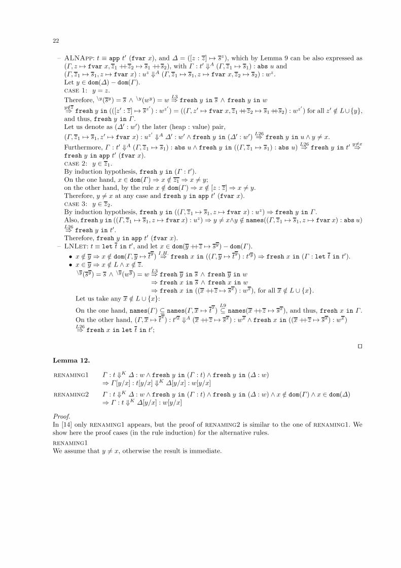
22
– ALNApp: t ≡ app t′ (fvar x), and ∆ = ([z : z] 7→ sz), which by Lemma 9 can be also expressed as(Γ, z 7→ fvar x, z1 ++z2 7→ s1 ++s2), with Γ : t′ ⇓A (Γ, z1 7→ s1) : abs u and(Γ, z1 7→ s1, z 7→ fvar x) : uz ⇓A (Γ, z1 7→ s1, z 7→ fvar x, z2 7→ s2) : wz .Let y ∈ dom(∆) − dom(Γ ).case 1: y = z.
Therefore, \y(sy) = s ∧ \y(wy) = wL3⇒ fresh y in s ∧ fresh y in w
y/∈z⇒ fresh y in (([z′ : z] 7→ sz′) : wz′
) = ((Γ, z′ 7→ fvar x, z1 ++z2 7→ s1 ++s2) : wz′) for all z′ /∈ L∪{y},
and thus, fresh y in Γ .Let us denote as (∆′ : w′) the later (heap : value) pair,
(Γ, z1 7→ s1, z′ 7→ fvar x) : uz′ ⇓A ∆′ : w′ ∧ fresh y in (∆′ : w′)
L26⇒ fresh y in u ∧ y 6= x.
Furthermore, Γ : t′ ⇓A (Γ, z1 7→ s1) : abs u ∧ fresh y in ((Γ, z1 7→ s1) : abs u)L26⇒ fresh y in t′
y 6=x⇒fresh y in app t′ (fvar x).case 2: y ∈ z1.By induction hypothesis, fresh y in (Γ : t′).On the one hand, x ∈ dom(Γ )⇒ x /∈ z1 ⇒ x 6= y;on the other hand, by the rule x /∈ dom(Γ )⇒ x /∈ [z : z]⇒ x 6= y.Therefore, y 6= x at any case and fresh y in app t′ (fvar x).case 3: y ∈ z2.By induction hypothesis, fresh y in ((Γ, z1 7→ s1, z 7→ fvar x) : uz)⇒ fresh y in Γ .Also, fresh y in ((Γ, z1 7→ s1, z 7→ fvar x) : uz)⇒ y 6= x∧y /∈ names((Γ, z1 7→ s1, z 7→ fvar x) : abs u)L26⇒ fresh y in t′.Therefore, fresh y in app t′ (fvar x).
– LNLet: t ≡ let t in t′, and let x ∈ dom(y ++z 7→ sy)− dom(Γ ).
• x /∈ y ⇒ x /∈ dom(Γ, y 7→ ty)I.H.⇒ fresh x in ((Γ, y 7→ t
y) : t′y)⇒ fresh x in (Γ : let t in t′).
• x ∈ y ⇒ x /∈ L ∧ x /∈ z.\y(sy) = s ∧ \y(wy) = w
L3⇒ fresh y in s ∧ fresh y in w⇒ fresh x in s ∧ fresh x in w⇒ fresh x in ((x ++z 7→ sx) : wx), for all x /∈ L ∪ {x}.
Let us take any x /∈ L ∪ {x}:On the one hand, names(Γ ) ⊆ names(Γ, x 7→ t
x)L9⊆ names(x ++z 7→ sx), and thus, fresh x in Γ .
On the other hand, (Γ, x 7→ tx) : t′x ⇓A (x ++z 7→ sx) : wx ∧ fresh x in ((x ++z 7→ sx) : wx)
L26⇒ fresh x in let t in t′;
⊓⊔
Lemma 12.
renaming1 Γ : t ⇓K ∆ : w ∧ fresh y in (Γ : t) ∧ fresh y in (∆ : w)⇒ Γ [y/x] : t[y/x] ⇓K ∆[y/x] : w[y/x]
renaming2 Γ : t ⇓K ∆ : w ∧ fresh y in (Γ : t) ∧ fresh y in (∆ : w) ∧ x /∈ dom(Γ ) ∧ x ∈ dom(∆)⇒ Γ : t ⇓K ∆[y/x] : w[y/x]
Proof.In [14] only renaming1 appears, but the proof of renaming2 is similar to the one of renaming1. Weshow here the proof cases (in the rule induction) for the alternative rules.
renaming1We assume that y 6= x, otherwise the result is immediate.
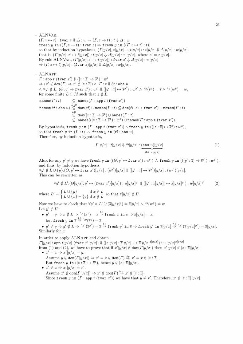
23
– ALNVar:(Γ, z 7→ t) : fvar z ⇓ ∆ : w⇒ (Γ, z 7→ t) : t ⇓ ∆ : w;fresh y in ((Γ, z 7→ t) : fvar z)⇒ fresh y in ((Γ, z 7→ t) : t),so that by induction hypothesis, (Γ [y/x], z[y/x] 7→ t[y/x]) : t[y/x] ⇓ ∆[y/x] : w[y/x],that is, (Γ [y/x], z′ 7→ t[y/x]) : t[y/x] ⇓ ∆[y/x] : w[y/x], where z′ = z[y/x].By rule ALNVar, (Γ [y/x], z′ 7→ t[y/x]) : fvar z′ ⇓ ∆[y/x] : w[y/x]⇒ (Γ, z 7→ t)[y/x] : (fvar z)[y/x] ⇓ ∆[y/x] : w[y/x].
– ALNApp:Γ : app t (fvar x′) ⇓ ([z : z] 7→ sz) : wz
⇒ (x′ /∈ dom(Γ )⇒ x′ /∈ [z : z]) ∧ Γ : t ⇓ Θ : abs u
∧ ∀y′ /∈ L. (Θ, y′ 7→ fvar x′) : uy′ ⇓ ([y′ : z] 7→ sy′) : wy′ ∧ \y(sy) = s ∧ \y(wy) = w,
for some finite L ⊆ Id such that z /∈ L.
names(Γ : t) ⊆ names(Γ : app t (fvar x′))
names(Θ : abs u)L10⊆ dom(Θ) ∪ names(Γ : t) ⊆ dom(Θ, z 7→ fvar x′) ∪ names(Γ : t)L8⊆ dom([z : z] 7→ sz) ∪ names(Γ : t)⊆ names(([z : z] 7→ sz) : wz) ∪ names(Γ : app t (fvar x′)).
By hypothesis, fresh y in (Γ : app t (fvar x′)) ∧ fresh y in (([z : z] 7→ sz) : wz),so that fresh y in (Γ : t) ∧ fresh y in (Θ : abs u).Therefore, by induction hypothesis,
Γ [y/x] : t[y/x] ⇓ Θ[y/x] : (abs u)[y/x]︸ ︷︷ ︸abs u[y/x]
(1)
Also, for any y′ 6= y we have fresh y in ((Θ, y′ 7→ fvar x′) : uy′) ∧ fresh y in (([y′ : z] 7→ sy
′) : wy′
),and thus, by induction hypothesis,∀y′ /∈ L ∪ {y}.(Θ, y′ 7→ fvar x′)[y/x] : (uy′
)[y/x] ⇓ ([y′ : z] 7→ sy′)[y/x] : (wy′
)[y/x].This can be rewritten as
∀y′ /∈ L′.(Θ[y/x], y′ 7→ (fvar x′)[y/x]) : u[y/x]y′ ⇓ ([y′ : z[y/x]] 7→ s[y/x]y
′) : w[y/x]y
′(2)
where L′ =
{L ∪ {y} if x ∈ LL ∪ {x} − {y} if x /∈ L
so that z[y/x] /∈ L′.
Now we have to check that ∀y′ /∈ L′.\y(s[y/x]y) = s[y/x] ∧ \y(wy) = w.Let y′ /∈ L′:• y′ = y ⇒ x /∈ L⇒ \x(sx) = s
L3⇒ fresh x in s⇒ s[y/x] = s;
but fresh y in sL3⇒ \y(sy) = s.
• y′ 6= y ⇒ y′ /∈ L⇒ \y′(sy
′) = s
L3⇒ fresh y′ in s⇒ fresh y′ in s[y/x]L3⇒ \y′
(s[y/x]y′) = s[y/x].
Similarly for w.
In order to apply ALNApp and obtainΓ [y/x] : app t[y/x] (fvar x′[y/x]) ⇓ ([z[y/x] : z[y/x]] 7→ s[y/x]z[y/x]) : w[y/x]z[y/x]
from (1) and (2), we have to prove that if x′[y/x] /∈ dom(Γ [y/x]) then x′[y/x] /∈ [z : z][y/x]:• x′ = x⇒ x′[y/x] = y.
Assume y /∈ dom(Γ [y/x])⇒ x′ = x /∈ dom(Γ )hip.⇒ x′ = x /∈ [z : z].
But fresh y in ([z : z] 7→ sz), hence y /∈ [z : z][y/x].• x′ 6= x⇒ x′[y/x] = x′.
Assume x′ /∈ dom(Γ [y/x])⇒ x′ /∈ dom(Γ )hip.⇒ x′ /∈ [z : z].
Since fresh y in (Γ : app t (fvar x′)) we have that y 6= x′. Therefore, x′ /∈ [z : z][y/x].

24
renaming2We assume that y 6= x, otherwise the result is immediate.By rule induction:
– ALNVar:The proof is similar to the corresponding case in renaming1.
– ALNApp:⇒ (x′ /∈ dom(Γ )⇒ x′ /∈ [z : z]) ∧ Γ : t ⇓ Θ : abs u
∧ ∀y′ /∈ L. (Θ, y′ 7→ fvar x′) : uy′ ⇓ ([y′ : z] 7→ sy′) : wy′ ∧ \y(sy) = s ∧ \y(wy) = w,
for some finite L ⊆ Id such that z /∈ L.
Following the same steps as in renaming1 we obtain that fresh y in (Θ : abs u), and that for any
y′ 6= y it is fresh y in ((Θ, y′ 7→ fvar x′) : uy′) ∧ fresh y in (([y′ : z] 7→ sy
′) : wy′
).Moreover, fresh y in (([z : z] 7→ sz) : wz)⇒ y 6= z ∧ y /∈ z,fresh y in (Γ : app t (fvar x′))⇒ y 6= x′, andx /∈ dom(Γ ) ∧ x ∈ dom([z : z] 7→ sz)⇒ x 6= x′.
case 1: x ∈ dom(Θ)On the one hand, by hypothesis x /∈ dom(Γ ), so that by induction hypothesis,
Γ : t ⇓ Θ[y/x] : (abs u)[y/x]︸ ︷︷ ︸abs u[y/x]
On the other hand, if we define L′ = L ∪ {y} we obtain
∀y′ /∈ L′.(Θ, y′ 7→ fvar x′) : uy′ ⇓ ([y′ : z] 7→ sy′) : wy′
and by using renaming1 we have
∀y′ /∈ L′.(Θ, y′ 7→ fvar x′)[y/x] : uy′[y/x] ⇓ ([y′ : z] 7→ sy
′)[y/x] : wy′
[y/x].
As we are assuming x ∈ dom(Θ), by Lemma 7 we have ∀y′ /∈ L′.y′ 6= x; particularly, z 6= x. This fact,together with x 6= x′ allows to rewrite the last equation as
∀y′ /∈ L′.(Θ[y/x], y′ 7→ fvar x′) : u[y/x]y′ ⇓ ([y′ : z][y/x] 7→ s[y/x]y
′) : w[y/x]y
′.
Take any y′ /∈ L′ ⇒ y′ /∈ L⇒ \y(sy) = sL3⇒ fresh y′ in s
y′ 6=y⇒ fresh y′ in s[y/x]L3⇒ \y(s[y/x]y) = s[y/x]
(similarly for w).
Furthermore, z /∈ L′, and x′ /∈ dom(Γ )⇒ x′ /∈ dom([z : z] 7→ sz)y 6=x′⇒ x′ /∈ dom([z : z][y/x] 7→ s[y/x]z).
Then by rule ALNApp,
Γ : app t (fvar x′) ⇓ ([z : z][y/x] 7→ s[y/x]z) : w[y/x]z
which, as z 6= x, can be rewritten to
Γ : app t (fvar x′) ⇓ ([z : z] 7→ sz)[y/x] : wz [y/x].
case 2: x /∈ dom(Θ)By hypothesis, Γ : t ⇓ Θ : abs u.We have to find a finite set L′ ⊆ Id such that z[y/x] /∈ L′,x′ /∈ dom(Γ )⇒ x′ /∈ dom([z : z][y/x] 7→ sz[y/x]), and
∀y′ /∈ L′.(Θ, y′ 7→ fvar x′) : uy′ ⇓ ([y′ : z[y/x]] 7→ s[y/x]y′) : w[y/x]y
′
and then apply the rule ALNApp.
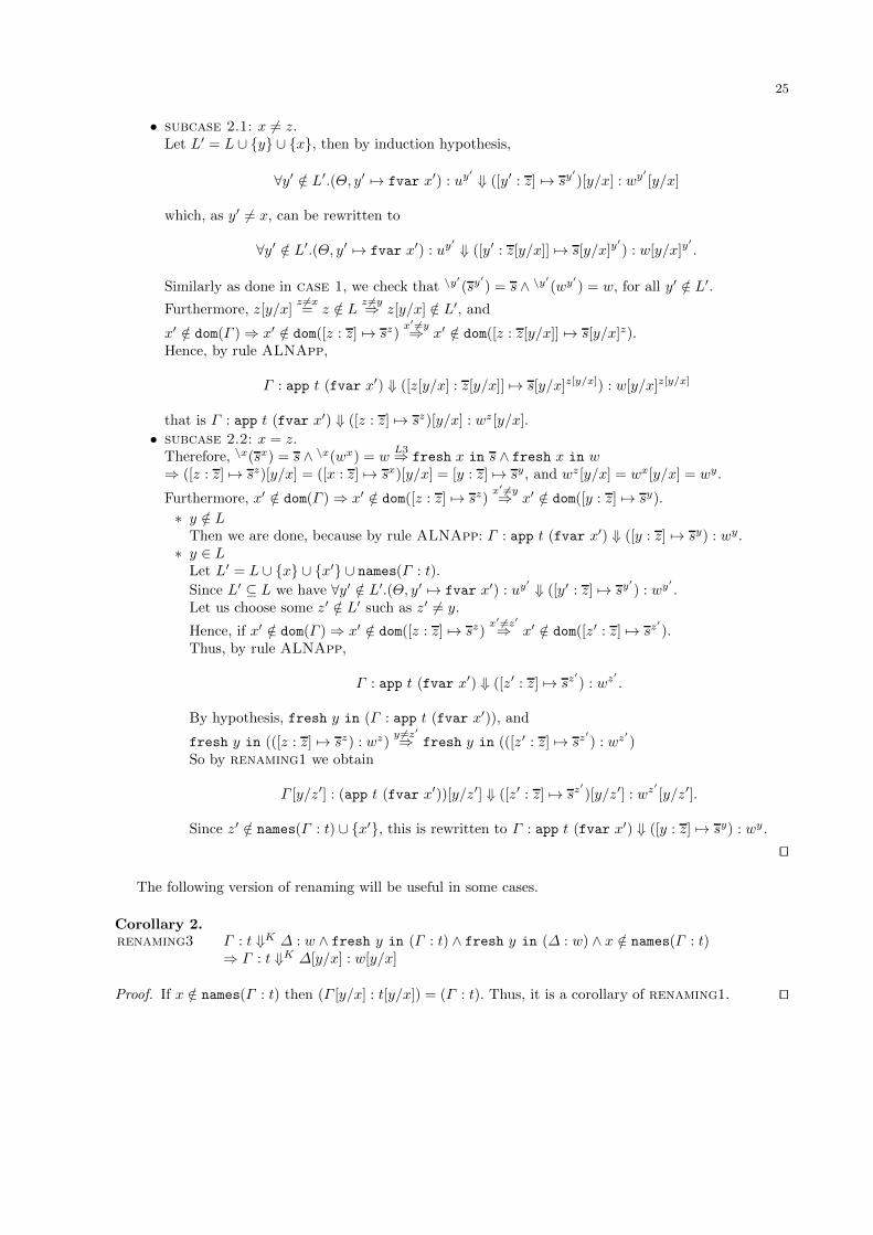
25
• subcase 2.1: x 6= z.Let L′ = L ∪ {y} ∪ {x}, then by induction hypothesis,
∀y′ /∈ L′.(Θ, y′ 7→ fvar x′) : uy′ ⇓ ([y′ : z] 7→ sy′)[y/x] : wy′
[y/x]
which, as y′ 6= x, can be rewritten to
∀y′ /∈ L′.(Θ, y′ 7→ fvar x′) : uy′ ⇓ ([y′ : z[y/x]] 7→ s[y/x]y′) : w[y/x]y
′.
Similarly as done in case 1, we check that \y′(sy
′) = s ∧ \y′
(wy′) = w, for all y′ /∈ L′.
Furthermore, z[y/x]z 6=x= z /∈ L
z 6=y⇒ z[y/x] /∈ L′, and
x′ /∈ dom(Γ )⇒ x′ /∈ dom([z : z] 7→ sz)x′ 6=y⇒ x′ /∈ dom([z : z[y/x]] 7→ s[y/x]z).
Hence, by rule ALNApp,
Γ : app t (fvar x′) ⇓ ([z[y/x] : z[y/x]] 7→ s[y/x]z[y/x]) : w[y/x]z[y/x]
that is Γ : app t (fvar x′) ⇓ ([z : z] 7→ sz)[y/x] : wz [y/x].
• subcase 2.2: x = z.Therefore, \x(sx) = s ∧ \x(wx) = w
L3⇒ fresh x in s ∧ fresh x in w⇒ ([z : z] 7→ sz)[y/x] = ([x : z] 7→ sx)[y/x] = [y : z] 7→ sy, and wz [y/x] = wx[y/x] = wy.
Furthermore, x′ /∈ dom(Γ )⇒ x′ /∈ dom([z : z] 7→ sz)x′ 6=y⇒ x′ /∈ dom([y : z] 7→ sy).
∗ y /∈ LThen we are done, because by rule ALNApp: Γ : app t (fvar x′) ⇓ ([y : z] 7→ sy) : wy.∗ y ∈ L
Let L′ = L ∪ {x} ∪ {x′} ∪ names(Γ : t).
Since L′ ⊆ L we have ∀y′ /∈ L′.(Θ, y′ 7→ fvar x′) : uy′ ⇓ ([y′ : z] 7→ sy′) : wy′
.Let us choose some z′ /∈ L′ such as z′ 6= y.
Hence, if x′ /∈ dom(Γ )⇒ x′ /∈ dom([z : z] 7→ sz)x′ 6=z′⇒ x′ /∈ dom([z′ : z] 7→ sz
′).
Thus, by rule ALNApp,
Γ : app t (fvar x′) ⇓ ([z′ : z] 7→ sz′) : wz′
.
By hypothesis, fresh y in (Γ : app t (fvar x′)), and
fresh y in (([z : z] 7→ sz) : wz)y 6=z′⇒ fresh y in (([z′ : z] 7→ sz
′) : wz′
)So by renaming1 we obtain
Γ [y/z′] : (app t (fvar x′))[y/z′] ⇓ ([z′ : z] 7→ sz′)[y/z′] : wz′
[y/z′].
Since z′ /∈ names(Γ : t) ∪ {x′}, this is rewritten to Γ : app t (fvar x′) ⇓ ([y : z] 7→ sy) : wy .
⊓⊔
The following version of renaming will be useful in some cases.
Corollary 2.renaming3 Γ : t ⇓K ∆ : w ∧ fresh y in (Γ : t) ∧ fresh y in (∆ : w) ∧ x /∈ names(Γ : t)
⇒ Γ : t ⇓K ∆[y/x] : w[y/x]
Proof. If x /∈ names(Γ : t) then (Γ [y/x] : t[y/x]) = (Γ : t). Thus, it is a corollary of renaming1. ⊓⊔
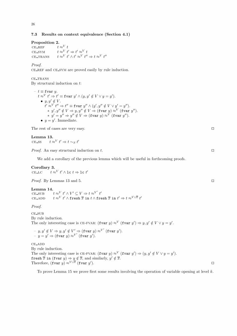
26
7.3 Results on context equivalence (Section 4.1)
Proposition 2.ce ref t ≈V tce sym t ≈V t′ ⇒ t′ ≈V tce trans t ≈V t′ ∧ t′ ≈V t′′ ⇒ t ≈V t′′
Proof.ce ref and ce sym are proved easily by rule induction.
ce transBy structural induction on t:
– t ≡ fvar y.t ≈V t′ ⇒ t′ ≡ fvar y′ ∧ (y, y′ /∈ V ∨ y = y′).• y, y′ /∈ V .t′ ≈V t′′ ⇒ t′′ ≡ fvar y′′ ∧ (y′, y′′ /∈ V ∨ y′ = y′′).∗ y′, y′′ /∈ V ⇒ y, y′′ /∈ V ⇒ (fvar y) ≈V (fvar y′′).∗ y′ = y′′ ⇒ y′′ /∈ V ⇒ (fvar y) ≈V (fvar y′′).
• y = y′. Immediate.
The rest of cases are very easy. ⊓⊔
Lemma 13.ce ss t ≈V t′ ⇒ t ∼S t′
Proof. An easy structural induction on t. ⊓⊔
We add a corollary of the previous lemma which will be useful in forthcoming proofs.
Corollary 3.ce lc t ≈V t′ ∧ lc t⇒ lc t′
Proof. By Lemmas 13 and 5. ⊓⊔
Lemma 14.ce sub t ≈V t′ ∧ V ′ ⊆ V ⇒ t ≈V ′
t′
ce add t ≈V t′ ∧ fresh x in t ∧ fresh x in t′ ⇒ t ≈V ∪x t′
Proof.
ce subBy rule induction.The only interesting case is ce-fvar: (fvar y) ≈V (fvar y′)⇒ y, y′ /∈ V ∨ y = y′.
– y, y′ /∈ V ⇒ y, y′ /∈ V ′ ⇒ (fvar y) ≈V ′(fvar y′).
– y = y′ ⇒ (fvar y) ≈V ′(fvar y′).
ce addBy rule induction.The only interesting case is ce-fvar: (fvar y) ≈V (fvar y′)⇒ (y, y′ /∈ V ∨ y = y′).fresh x in (fvar y)⇒ y /∈ x, and similarly, y′ /∈ x.Therefore, (fvar y) ≈V ∪x (fvar y′). ⊓⊔
To prove Lemma 15 we prove first some results involving the operation of variable opening at level k.
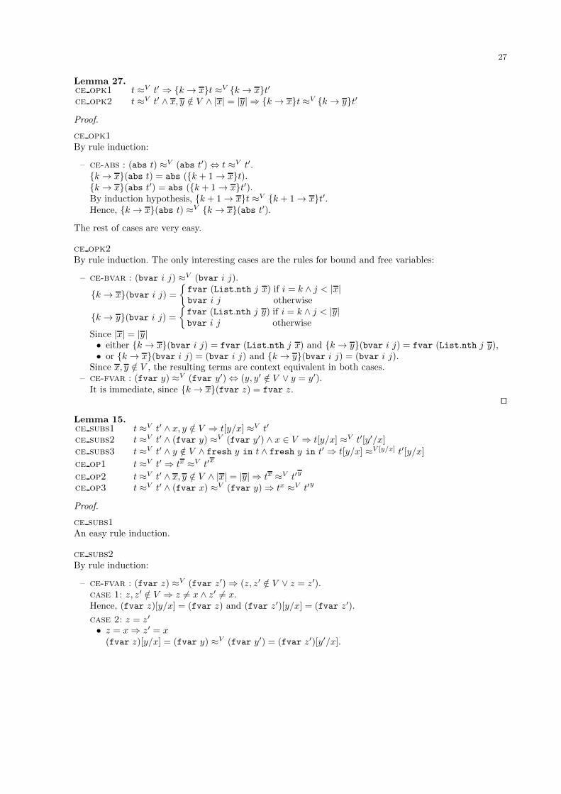
27
Lemma 27.ce opk1 t ≈V t′ ⇒ {k→ x}t ≈V {k→ x}t′ce opk2 t ≈V t′ ∧ x, y /∈ V ∧ |x| = |y| ⇒ {k→ x}t ≈V {k→ y}t′
Proof.
ce opk1By rule induction:
– ce-abs : (abs t) ≈V (abs t′)⇔ t ≈V t′.{k→ x}(abs t) = abs ({k + 1→ x}t).{k→ x}(abs t′) = abs ({k + 1→ x}t′).By induction hypothesis, {k + 1→ x}t ≈V {k + 1→ x}t′.Hence, {k→ x}(abs t) ≈V {k → x}(abs t′).
The rest of cases are very easy.
ce opk2By rule induction. The only interesting cases are the rules for bound and free variables:
– ce-bvar : (bvar i j) ≈V (bvar i j).
{k → x}(bvar i j) =
{fvar (List.nth j x) if i = k ∧ j < |x|bvar i j otherwise
{k → y}(bvar i j) =
{fvar (List.nth j y) if i = k ∧ j < |y|bvar i j otherwise
Since |x| = |y|• either {k → x}(bvar i j) = fvar (List.nth j x) and {k→ y}(bvar i j) = fvar (List.nth j y),• or {k→ x}(bvar i j) = (bvar i j) and {k → y}(bvar i j) = (bvar i j).
Since x, y /∈ V , the resulting terms are context equivalent in both cases.– ce-fvar : (fvar y) ≈V (fvar y′)⇔ (y, y′ /∈ V ∨ y = y′).
It is immediate, since {k→ x}(fvar z) = fvar z.⊓⊔
Lemma 15.ce subs1 t ≈V t′ ∧ x, y /∈ V ⇒ t[y/x] ≈V t′
ce subs2 t ≈V t′ ∧ (fvar y) ≈V (fvar y′) ∧ x ∈ V ⇒ t[y/x] ≈V t′[y′/x]
ce subs3 t ≈V t′ ∧ y /∈ V ∧ fresh y in t ∧ fresh y in t′ ⇒ t[y/x] ≈V [y/x] t′[y/x]
ce op1 t ≈V t′ ⇒ tx ≈V t′x
ce op2 t ≈V t′ ∧ x, y /∈ V ∧ |x| = |y| ⇒ tx ≈V t′y
ce op3 t ≈V t′ ∧ (fvar x) ≈V (fvar y)⇒ tx ≈V t′y
Proof.
ce subs1An easy rule induction.
ce subs2By rule induction:
– ce-fvar : (fvar z) ≈V (fvar z′)⇒ (z, z′ /∈ V ∨ z = z′).case 1: z, z′ /∈ V ⇒ z 6= x ∧ z′ 6= x.Hence, (fvar z)[y/x] = (fvar z) and (fvar z′)[y/x] = (fvar z′).
case 2: z = z′
• z = x⇒ z′ = x(fvar z)[y/x] = (fvar y) ≈V (fvar y′) = (fvar z′)[y′/x].
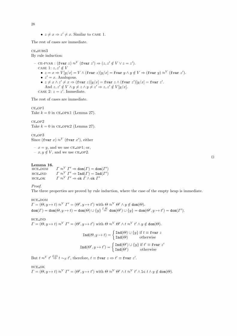
28
• z 6= x⇒ z′ 6= x. Similar to case 1.
The rest of cases are immediate.
ce subs3By rule induction:
– ce-fvar : (fvar z) ≈V (fvar z′)⇒ (z, z′ /∈ V ∨ z = z′).case 1: z, z′ /∈ V• z = x⇒ V [y/x] = V ∧ (fvar z)[y/x] = fvar y ∧ y /∈ V ⇒ (fvar y) ≈V (fvar z′).• z′ = x. Analogous.• z 6= x ∧ z′ 6= x⇒ (fvar z)[y/x] = fvar z ∧ (fvar z′)[y/x] = fvar z′.
And z, z′ /∈ V ∧ y 6= z ∧ y 6= z′ ⇒ z, z′ /∈ V [y/x].case 2: z = z′. Immediate.
The rest of cases are immediate.
ce op1Take k = 0 in ce opk1 (Lemma 27).
ce op2Take k = 0 in ce opk2 (Lemma 27).
ce op3Since (fvar x) ≈V (fvar x′), either
– x = y, and we use ce op1; or,– x, y /∈ V , and we use ce op2.
⊓⊔
Lemma 16.hce dom Γ ≈V Γ ′ ⇒ dom(Γ ) = dom(Γ ′)hce ind Γ ≈V Γ ′ ⇒ Ind(Γ ) = Ind(Γ ′)hce ok Γ ≈V Γ ′ ⇒ ok Γ ∧ ok Γ ′
Proof.The three properties are proved by rule induction, where the case of the empty heap is immediate.
hce domΓ = (Θ, y 7→ t) ≈V Γ ′ = (Θ′, y 7→ t′) with Θ ≈V Θ′ ∧ y /∈ dom(Θ).
dom(Γ ) = dom(Θ, y 7→ t) = dom(Θ) ∪ {y} I.H.= dom(Θ′) ∪ {y} = dom(Θ′, y 7→ t′) = dom(Γ ′).
hce indΓ = (Θ, y 7→ t) ≈V Γ ′ = (Θ′, y 7→ t′) with Θ ≈V Θ′ ∧ t ≈V t′ ∧ y /∈ dom(Θ).
Ind(Θ, y 7→ t) =
{Ind(Θ) ∪ {y} if t ≡ fvar zInd(Θ) otherwise
Ind(Θ′, y 7→ t′) =
{Ind(Θ′) ∪ {y} if t′ ≡ fvar z′
Ind(Θ′) otherwise
But t ≈V t′L13⇒ t ∼S t′, therefore, t ≡ fvar z ⇔ t′ ≡ fvar z′.
hce okΓ = (Θ, y 7→ t) ≈V Γ ′ = (Θ′, y 7→ t′) with Θ ≈V Θ′ ∧ t ≈V t′ ∧ lc t ∧ y /∈ dom(Θ).

29
Θ ≈V Θ′ I.H.⇒ ok Θ ∧ ok Θ′.lc t
C3⇒ lc t′.y /∈ dom(Θ)
hce dom= dom(Θ′).
Thus, ok (Θ, y 7→ t) and ok (Θ′, y 7→ t′). ⊓⊔
To prove that ≈V is an equivalence on heaps, we prove first that the relation is independent of theorder in which the bindings of the heaps are considered. So that when two heaps are related (in somecontext), all the names defined in those heaps are related.
Lemma 28.hce bind (Γ, x 7→ t) ≈V (Γ ′, x 7→ t′)⇒ Γ ≈V Γ ′ ∧ t ≈V t′
Proof. By induction on the size of Γ .
– Γ = ∅.(∅, x 7→ t) ≈V (Γ ′, x 7→ t′)⇒ Γ = ∅ ≈V Γ ′ ∧ t ≈V t′ ∧ lc t.
– Γ 6= ∅.Let ∆ = (Γ, x 7→ t) and ∆′ = (Γ ′, x 7→ t′).∆ ≈V ∆′ ⇒ ∃y.∆ = (Θ, y 7→ ty) ∧∆′ = (Θ′, y 7→ t′y) ∧Θ ≈V Θ′ ∧ ty ≈V t′y ∧ lc ty.If y = x then by hce ok in Lemma 16 there is a unique x in ∆ and ∆′, so that Γ = Θ ∧ Γ ′ = Θ′, andwe are done.Otherwise, Θ = (Θx, x 7→ t) and Θ′ = (Θ′
x, x 7→ t′), being (Θx, y 7→ ty) = Γ , and hence Θx ( Γ .By induction hypotesis, Θx ≈V Θ′
x ∧ t ≈V t′ ∧ lc t.Furthermore, Θx ≈V Θ′
x ∧ ty ≈V t′y ∧ lc ty ⇒ Γ = (Θx, y 7→ ty) ≈V (Θ′x, y 7→ t′y) = Γ ′.
⊓⊔
Proposition 3hce ref ok Γ ⇒ Γ ≈V Γhce sym Γ ≈V Γ ′ ⇒ Γ ′ ≈V Γhce trans Γ ≈V Γ ′ ∧ Γ ′ ≈V Γ ′′ ⇒ Γ ≈V Γ ′′
Proof.hce ref and hce sym are immediate.
hce transBy rule induction on Γ ≈V Γ ′:
– hce empty. ∅ ≈V ∅ ⇒ Γ ′′ = ∅. Immediate.
– hce cons. Γ = (Θ, y 7→ t) ≈V Γ ′ = (Θ′, y 7→ t′)⇒ Θ ≈V Θ′ ∧ t ≈V t′ ∧ lc t ∧ y /∈ dom(Θ)
Γ ′ ≈V Γ ′′ L16⇒ dom(Γ ′) = dom(Γ ′′)⇒ Γ ′′ = (Θ′′, y 7→ t′′)L28⇒ Θ′ ≈V Θ′′ ∧ t′ ≈V t′′.
By induction hypothesis, Θ ≈V Θ′′.By ce trans in Proposition 2, t ≈V t′′.Hence, Γ = (Θ, y 7→ t) ≈V (Θ′′, y 7→ t′′) = Γ ′′.
⊓⊔
Lemma 17hce alt Γ ≈V Γ ′ ⇔ ok Γ ∧ ok Γ ′ ∧ dom(Γ ) = dom(Γ ′) ∧ (x 7→ t ∈ Γ ∧ x 7→ t′ ∈ Γ ′ ⇒ t ≈V t′)
Proof.⇒ By hce dom and hce ok (Lemma 16) and hce bind (Lemma 28).
⇐ By induction on the size of Γ :

30
– Γ = ∅. Immediate.– Γ = (Θ, y 7→ ty)⇒ Γ ′ = (Θ′, y 7→ t′y) ∧ dom(Θ) = dom(Θ′) ∧ ty ≈V t′y.ok Γ ⇒ ok Θ ∧ y /∈ dom(Θ) ∧ lc ty,ok Γ ′ ⇒ ok Θ′ ∧ y /∈ dom(Θ′) ∧ lc t′y.If x 7→ t ∈ Θ ⊆ Γ ∧ x 7→ t′ ∈ Θ′ ⊆ Γ ′ then t ≈V t′.Hence ok Θ ∧ ok Θ′ ∧ dom(Θ) = dom(Θ′) ∧ (x 7→ t ∈ Θ ∧ x 7→ t′ ∈ Θ′ ⇒ t ≈V t′).By induction hypothesis, Θ ≈V Θ′.Thus, Γ = (Θ, y 7→ ty) ≈V (Θ′, x 7→ t′y) = Γ ′.
⊓⊔
The following auxiliary result is used in the proofs of the Lemmas 18 and 19:
Lemma 29.ind dom ok Γ ∧ x ∈ Ind(Γ )⇒ dom(Γ ⊖ x) = dom(Γ )− {x} ∧ Ind(Γ ⊖ x) = Ind(Γ )− {x}
Proof.An easy induction on the size of Γ . ⊓⊔
We also give here some other properties related to the deletion of indirections. These will be used inforthcoming proofs.
Lemma 30.ind ok ok Γ ∧ x ∈ Ind(Γ )⇒ ok (Γ ⊖ x)
Proof. Γ = (Θ, x 7→ fvar y).ok Γ ⇒ ok Θ ∧ x /∈ dom(Θ).By induction on the size of Θ:
– Θ = ∅.Γ ⊖ x = ∅. Immediate.
– Θ = (∆, z 7→ t).Γ ⊖ x = ((∆,x 7→ fvar y)⊖ x, z 7→ t[y/x]).ok Θ⇒ ok ∆ ∧ z /∈ dom(∆) ∧ lc t.
z /∈ dom(∆)L29= dom((∆,x 7→ fvar y)⊖ x).
lc t⇒ lc t[y/x].ok ∆x /∈ dom(Θ)⇒ x /∈ dom(∆)lc (fvar y)
⇒ ok (∆,x 7→ fvar y)
I.H.⇒ ok ((∆,x 7→ fvar y)⊖ x).
Therefore ok ((∆,x 7→ fvar y))⊖ x, z 7→ t[y/x])⇒ ok (Γ ⊖ x).⊓⊔
Lemma 31.ind subs x /∈ dom(Γ )⇒ (Γ, x 7→ fvar y)⊖ x = Γ [y/x]
Proof.An easy induction on the size of Γ . ⊓⊔
Lemma 18hce swap ok Γ ∧ x, y ∈ Ind(Γ ) ∧ x 6= y ⇒ Γ ⊖ [x, y] ≈V −{x,y} Γ ⊖ [y, x]
Proof.We have Γ = (Θ, x 7→ fvar x′, y 7→ fvar y′).By induction on the size of Θ:
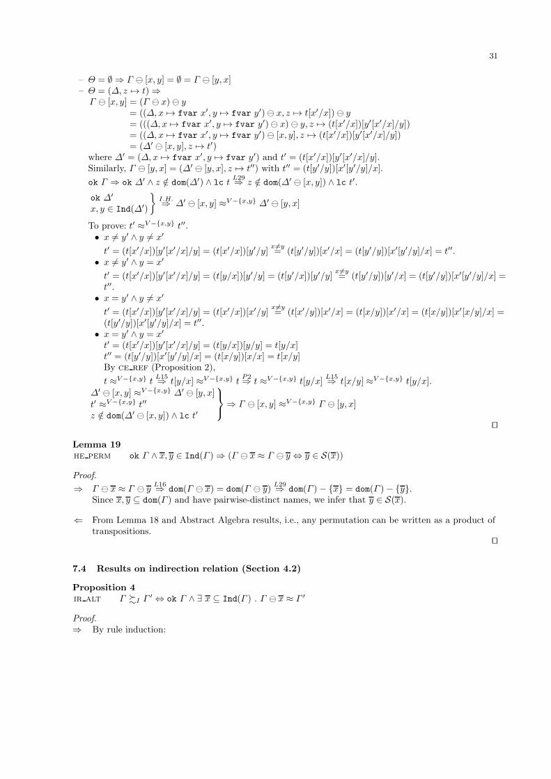
31
– Θ = ∅ ⇒ Γ ⊖ [x, y] = ∅ = Γ ⊖ [y, x]– Θ = (∆, z 7→ t)⇒
Γ ⊖ [x, y] = (Γ ⊖ x)⊖ y= ((∆,x 7→ fvar x′, y 7→ fvar y′)⊖ x, z 7→ t[x′/x])⊖ y= (((∆,x 7→ fvar x′, y 7→ fvar y′)⊖ x) ⊖ y, z 7→ (t[x′/x])[y′[x′/x]/y])= ((∆,x 7→ fvar x′, y 7→ fvar y′)⊖ [x, y], z 7→ (t[x′/x])[y′[x′/x]/y])= (∆′ ⊖ [x, y], z 7→ t′)
where ∆′ = (∆,x 7→ fvar x′, y 7→ fvar y′) and t′ = (t[x′/x])[y′[x′/x]/y].Similarly, Γ ⊖ [y, x] = (∆′ ⊖ [y, x], z 7→ t′′) with t′′ = (t[y′/y])[x′[y′/y]/x].
ok Γ ⇒ ok ∆′ ∧ z /∈ dom(∆′) ∧ lc tL29⇒ z /∈ dom(∆′ ⊖ [x, y]) ∧ lc t′.
ok ∆′
x, y ∈ Ind(∆′)
}I.H.⇒ ∆′ ⊖ [x, y] ≈V −{x,y} ∆′ ⊖ [y, x]
To prove: t′ ≈V−{x,y} t′′.• x 6= y′ ∧ y 6= x′
t′ = (t[x′/x])[y′[x′/x]/y] = (t[x′/x])[y′/y]x 6=y= (t[y′/y])[x′/x] = (t[y′/y])[x′[y′/y]/x] = t′′.
• x 6= y′ ∧ y = x′
t′ = (t[x′/x])[y′[x′/x]/y] = (t[y/x])[y′/y] = (t[y′/x])[y′/y]x 6=y= (t[y′/y])[y′/x] = (t[y′/y])[x′[y′/y]/x] =
t′′.• x = y′ ∧ y 6= x′
t′ = (t[x′/x])[y′[x′/x]/y] = (t[x′/x])[x′/y]x 6=y= (t[x′/y])[x′/x] = (t[x/y])[x′/x] = (t[x/y])[x′[x/y]/x] =
(t[y′/y])[x′[y′/y]/x] = t′′.• x = y′ ∧ y = x′
t′ = (t[x′/x])[y′[x′/x]/y] = (t[y/x])[y/y] = t[y/x]t′′ = (t[y′/y])[x′[y′/y]/x] = (t[x/y])[x/x] = t[x/y]By ce ref (Proposition 2),
t ≈V−{x,y} tL15⇒ t[y/x] ≈V−{x,y} t
P2⇒ t ≈V−{x,y} t[y/x]L15⇒ t[x/y] ≈V−{x,y} t[y/x].
∆′ ⊖ [x, y] ≈V −{x,y} ∆′ ⊖ [y, x]
t′ ≈V−{x,y} t′′
z /∈ dom(∆′ ⊖ [x, y]) ∧ lc t′
⇒ Γ ⊖ [x, y] ≈V−{x,y} Γ ⊖ [y, x]
⊓⊔
Lemma 19he perm ok Γ ∧ x, y ∈ Ind(Γ )⇒ (Γ ⊖ x ≈ Γ ⊖ y ⇔ y ∈ S(x))
Proof.
⇒ Γ ⊖ x ≈ Γ ⊖ yL16⇒ dom(Γ ⊖ x) = dom(Γ ⊖ y)
L29⇒ dom(Γ )− {x} = dom(Γ )− {y}.Since x, y ⊆ dom(Γ ) and have pairwise-distinct names, we infer that y ∈ S(x).
⇐ From Lemma 18 and Abstract Algebra results, i.e., any permutation can be written as a product oftranspositions.
⊓⊔
7.4 Results on indirection relation (Section 4.2)
Proposition 4ir alt Γ %I Γ ′ ⇔ ok Γ ∧ ∃ x ⊆ Ind(Γ ) . Γ ⊖ x ≈ Γ ′
Proof.⇒ By rule induction:
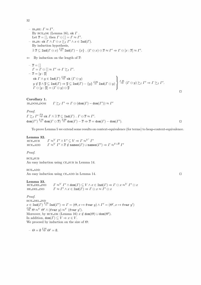
32
– ir he: Γ ≈ Γ ′.By hce ok (Lemma 16), ok Γ .Let x = [ ], then Γ ⊖ [ ] = Γ ≈ Γ ′.
– ir ir: ok Γ ∧ Γ ⊖ x %I Γ ′ ∧ x ∈ Ind(Γ ).By induction hypothesis,
∃ x ⊆ Ind(Γ ⊖ x)L29= Ind(Γ )− {x} . (Γ ⊖ x)⊖ x ≈ Γ ′ ⇒ Γ ⊖ [x : x] ≈ Γ ′.
⇐ By induction on the length of x:
– x = [ ]Γ = Γ ⊖ [ ] ≈ Γ ′ ⇒ Γ %I Γ ′.
– x = [y : y]
ok Γ ∧ y ∈ Ind(Γ )L30⇒ ok (Γ ⊖ y)
y /∈ y ∧ y ⊆ Ind(Γ )⇒ y ⊆ Ind(Γ )− {y} L29= Ind(Γ ⊖ y)
Γ ⊖ [y : y] = (Γ ⊖ y)⊖ y
I.H.⇒ (Γ ⊖ y) %I Γ ′ ⇒ Γ %I Γ ′.
⊓⊔
Corollary 1.ir dom dom Γ %I Γ ′ ⇒ Γ ⊖ (dom(Γ )− dom(Γ ′)) ≈ Γ ′
Proof.
Γ %I Γ ′ P4⇒ ok Γ ∧ ∃ x ⊆ Ind(Γ ) . Γ ⊖ x ≈ Γ ′.
dom(Γ ′)L16= dom(Γ ⊖ x)
L29= dom(Γ )− x⇒ x = dom(Γ )− dom(Γ ′). ⊓⊔
To prove Lemma 5 we extend some results on context-equivalence (for terms) to heap-context-equivalence.
Lemma 32.hce sub Γ ≈V Γ ′ ∧ V ′ ⊆ V ⇒ Γ ≈V ′
Γ ′
hce add Γ ≈V Γ ′ ∧ x /∈ names(Γ ) ∪ names(Γ ′)⇒ Γ ≈V ∪x Γ ′
Proof.
hce subAn easy induction using ce sub in Lemma 14.
hce addAn easy induction using ce add in Lemma 14. ⊓⊔
Lemma 33.hce del ind Γ ≈V Γ ′ ∧ dom(Γ ) ⊆ V ∧ x ∈ Ind(Γ )⇒ Γ ⊖ x ≈V Γ ′ ⊖ xhe del ind Γ ≈ Γ ′ ∧ x ∈ Ind(Γ )⇒ Γ ⊖ x ≈ Γ ′ ⊖ x
Proof.hce del indx ∈ Ind(Γ )
L16= Ind(Γ ′)⇒ Γ = (Θ, x 7→ fvar y) ∧ Γ ′ = (Θ′, x 7→ fvar y′)
L28⇒ Θ ≈V Θ′ ∧ (fvar y) ≈V (fvar y′).Moreover, by hce ok (Lemma 16) x /∈ dom(Θ) ∪ dom(Θ′).In addition, dom(Γ ) ⊆ V ⇒ x ∈ V .We proceed by induction on the size of Θ:
– Θ = ∅ L16⇒ Θ′ = ∅.

33
– Θ = (∆, z 7→ t) with z 6= x.By Lemma 16, Θ′ = (∆′, z 7→ t′).By Lemma 28, ∆ ≈V ∆′ ∧ t ≈V t′.
Therefore, (∆,x 7→ fvar y) ≈V (∆′, x 7→ fvar y′)I.H.⇒ (∆,x 7→ fvar y)⊖ x ≈V (∆′, x 7→ fvar y′)⊖ x.
Moreover, t ≈V t′ ∧ (fvar y) ≈V (fvar y′) ∧ x ∈ VL15⇒ t[y/x] ≈V t′[y′/x], lc t ⇒ lc t[y/x], and
z /∈ dom(∆,x 7→ fvar y).Hence, ((∆,x 7→ fvar y)⊖ x, z 7→ t[y/x]) ≈V ((∆′, x 7→ fvar y′)⊖ x, z 7→ t′[y′/x]).But Γ ⊖ x = ((∆,x 7→ fvar y)⊖ x, z 7→ t[y/x]) and Γ ′ ⊖ x = ((∆′, x 7→ fvar y′)⊖ x, z 7→ t′[y′/x]).
he del indIt is a direct consequence of hce del ind and Lemma 32. ⊓⊔
Proposition 5.ir ref ok Γ ⇒ Γ %I Γir trans Γ %I Γ ′ ∧ Γ ′ %I Γ ′′ ⇒ Γ %I Γ ′′
Proof.ir refBy hce ref in Proposition 3.
ir transBy rule induction on Γ %I Γ ′:
– Γ ≈ Γ ′.Γ ′ %I Γ ′′ P4⇒ ok Γ ′ ∧ ∃ x ⊆ Ind(Γ ′) . Γ ′ ⊖ x ≈ Γ ′′.By hce ind (Lemma 16), x ⊆ Ind(Γ ).By he del ind (Lemma 33), Γ ⊖ x ≈ Γ ′ ⊖ x and, by transitivity of ≈ (Proposition 3), Γ ⊖ x ≈ Γ ′′.By Proposition 4 (in the other direction) we get Γ %I Γ ′′.
– Γ ⊖ y %I Γ ′ ∧ y ∈ Ind(Γ ) ∧ ok Γ .By induction hypothesis Γ ⊖ y %I Γ ′′ ⇒ Γ %I Γ ′′.
⊓⊔
Lemma 20ir dom Γ %I Γ ′ ⇒ dom(Γ ′) ⊆ dom(Γ )ir ind Γ %I Γ ′ ⇒ Ind(Γ ′) ⊆ Ind(Γ )ir ok Γ %I Γ ′ ⇒ ok Γ ∧ ok Γ ′
ir dom he Γ %I Γ ′ ∧ dom(Γ ) = dom(Γ ′)⇒ Γ ≈ Γ ′
ir ir he (Γ %I Γ ′ ∧ Γ ′ %I Γ )⇔ Γ ≈ Γ ′
Proof.
The proofs of ir dom, ir ind and ir ok are easy rule inductions.
ir dom heWe prove by contrapositive: Assume Γ %I Γ ′ ∧ Γ ≈/ Γ ′.Γ %I Γ ′ ⇒ ok Γ ∧ Γ ⊖ x %I Γ ′ ∧ x ∈ Ind(Γ ).
By ir dom, dom(Γ ′) ⊆ dom(Γ ⊖ x)L29= dom(Γ )− {x} ( dom(Γ ).
Hence dom(Γ ) 6= dom(Γ ′).
ir ir he
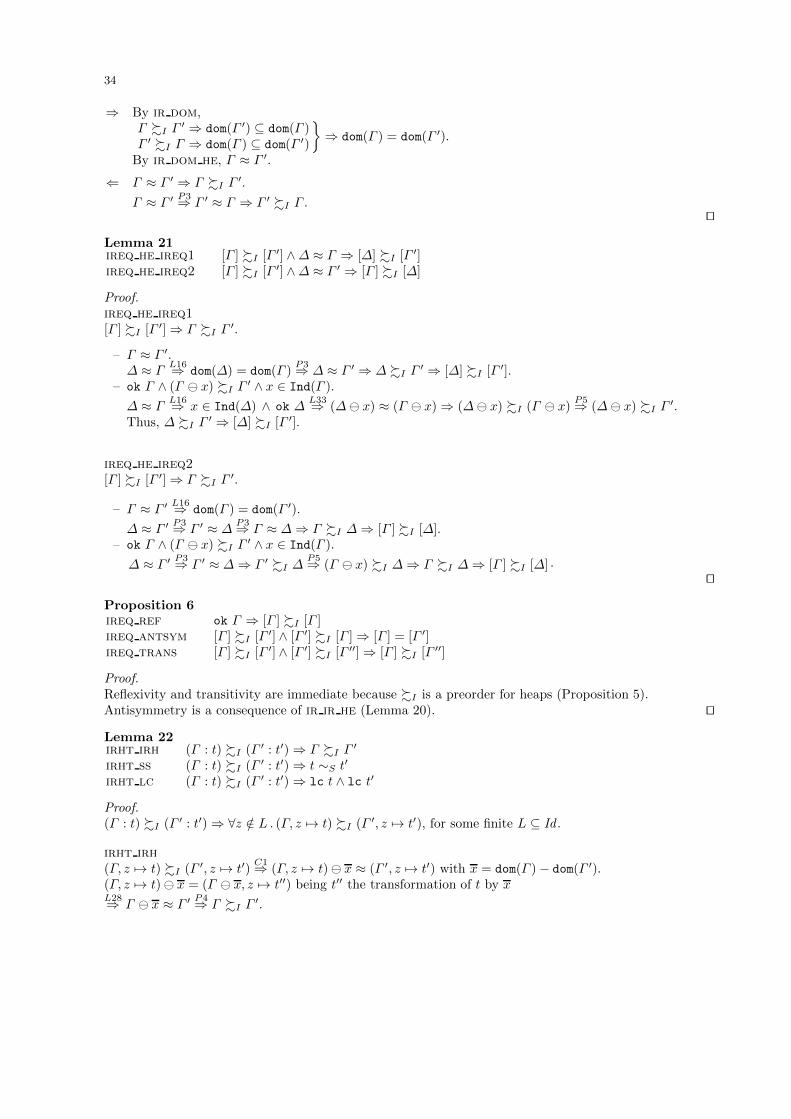
34
⇒ By ir dom,Γ %I Γ ′ ⇒ dom(Γ ′) ⊆ dom(Γ )Γ ′ %I Γ ⇒ dom(Γ ) ⊆ dom(Γ ′)
}⇒ dom(Γ ) = dom(Γ ′).
By ir dom he, Γ ≈ Γ ′.
⇐ Γ ≈ Γ ′ ⇒ Γ %I Γ ′.
Γ ≈ Γ ′ P3⇒ Γ ′ ≈ Γ ⇒ Γ ′ %I Γ .⊓⊔
Lemma 21ireq he ireq1 [Γ ] %I [Γ ′] ∧∆ ≈ Γ ⇒ [∆] %I [Γ ′]ireq he ireq2 [Γ ] %I [Γ ′] ∧∆ ≈ Γ ′ ⇒ [Γ ] %I [∆]
Proof.ireq he ireq1[Γ ] %I [Γ ′]⇒ Γ %I Γ ′.
– Γ ≈ Γ ′.∆ ≈ Γ
L16⇒ dom(∆) = dom(Γ )P3⇒ ∆ ≈ Γ ′ ⇒ ∆ %I Γ ′ ⇒ [∆] %I [Γ ′].
– ok Γ ∧ (Γ ⊖ x) %I Γ ′ ∧ x ∈ Ind(Γ ).
∆ ≈ ΓL16⇒ x ∈ Ind(∆) ∧ ok ∆
L33⇒ (∆⊖ x) ≈ (Γ ⊖ x)⇒ (∆⊖ x) %I (Γ ⊖ x)P5⇒ (∆⊖ x) %I Γ ′.
Thus, ∆ %I Γ ′ ⇒ [∆] %I [Γ ′].
ireq he ireq2[Γ ] %I [Γ ′]⇒ Γ %I Γ ′.
– Γ ≈ Γ ′ L16⇒ dom(Γ ) = dom(Γ ′).
∆ ≈ Γ ′ P3⇒ Γ ′ ≈ ∆P3⇒ Γ ≈ ∆⇒ Γ %I ∆⇒ [Γ ] %I [∆].
– ok Γ ∧ (Γ ⊖ x) %I Γ ′ ∧ x ∈ Ind(Γ ).
∆ ≈ Γ ′ P3⇒ Γ ′ ≈ ∆⇒ Γ ′ %I ∆P5⇒ (Γ ⊖ x) %I ∆⇒ Γ %I ∆⇒ [Γ ] %I [∆] .
⊓⊔
Proposition 6ireq ref ok Γ ⇒ [Γ ] %I [Γ ]ireq antsym [Γ ] %I [Γ ′] ∧ [Γ ′] %I [Γ ]⇒ [Γ ] = [Γ ′]ireq trans [Γ ] %I [Γ ′] ∧ [Γ ′] %I [Γ ′′]⇒ [Γ ] %I [Γ ′′]
Proof.Reflexivity and transitivity are immediate because %I is a preorder for heaps (Proposition 5).Antisymmetry is a consequence of ir ir he (Lemma 20). ⊓⊔
Lemma 22irht irh (Γ : t) %I (Γ ′ : t′)⇒ Γ %I Γ ′
irht ss (Γ : t) %I (Γ ′ : t′)⇒ t ∼S t′
irht lc (Γ : t) %I (Γ ′ : t′)⇒ lc t ∧ lc t′
Proof.(Γ : t) %I (Γ ′ : t′)⇒ ∀z /∈ L . (Γ, z 7→ t) %I (Γ ′, z 7→ t′), for some finite L ⊆ Id .
irht irh(Γ, z 7→ t) %I (Γ ′, z 7→ t′)
C1⇒ (Γ, z 7→ t)⊖ x ≈ (Γ ′, z 7→ t′) with x = dom(Γ )− dom(Γ ′).(Γ, z 7→ t)⊖ x = (Γ ⊖ x, z 7→ t′′) being t′′ the transformation of t by xL28⇒ Γ ⊖ x ≈ Γ ′ P4⇒ Γ %I Γ ′.
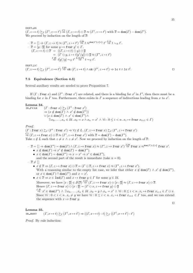
35
irht ss(Γ, z 7→ t) %I (Γ ′, z 7→ t′)
C1⇒ (Γ, z 7→ t)⊖ x ≈ (Γ ′, z 7→ t′) with x = dom(Γ )− dom(Γ ′).We proceed by induction on the length of x:
– x = [ ]⇒ (Γ, z 7→ t) ≈ (Γ ′, z 7→ t′)L28⇒ t ≈dom(Γ )∪{z} t′
L13⇒ t ∼S t′.– x = [y : y] for some y 7→ fvar y′ ∈ Γ .
(Γ, z 7→ t)⊖ x = ((Γ, z 7→ t)⊖ y)⊖ y= (Γ ⊖ y, z 7→ t[y′/y])⊖ y ≈ (Γ ′, z 7→ t′)
I.H.⇒ t[y′/y] ∼S t′L1&P1⇒ t ∼S t′.
irht lc(Γ, z 7→ t) %I (Γ ′, z 7→ t′)
L20⇒ ok (Γ, z 7→ t) ∧ ok (Γ ′, z 7→ t′)⇒ lc t ∧ lc t′. ⊓⊔
7.5 Equivalence (Section 4.3)
Several auxiliary results are needed to prove Proposition 7.
If (Γ : fvar x) and (Γ ′ : fvar x′) are related, and there is a binding for x′ in Γ ′, then there must be abinding for x in Γ too. Furthermore, there exists in Γ a sequence of indirections leading from x to x′.
Lemma 34.ir fvar (Γ : fvar x) %I (Γ ′ : fvar x′)
⇒ (x /∈ dom(Γ ) ∧ x′ /∈ dom(Γ ′))∨ (x ∈ dom(Γ ) ∧ x′ ∈ dom(Γ ′)∧∃x0, . . . , xn ∈ Id . x0 = x ∧ xn = x′ ∧ ∀i : 0 ≤ i < n . xi 7→ fvar xi+1 ∈ Γ )
Proof.(Γ : fvar x) %I (Γ ′ : fvar x′)⇒ ∀z /∈ L . (Γ, z 7→ fvar x) %I (Γ ′, z 7→ fvar x′)C1⇒ (Γ, z 7→ fvar x) ⊖ x ≈ (Γ ′, z 7→ fvar x′) with x = dom(Γ )− dom(Γ ′).Take z /∈ L such that z 6= x ∧ z 6= x′. Now we proceed by induction on the length of x:
– x = [ ]⇒ dom(Γ ′) = dom(Γ ) ∧ (Γ, z 7→ fvar x) ≈ (Γ ′, z 7→ fvar x′)L28⇒ fvar x ≈dom(Γ )∪{z} fvar x′.
• x /∈ dom(Γ )⇒ x′ /∈ dom(Γ ) = dom(Γ ′).• x ∈ dom(Γ ) = dom(Γ ′)⇒ x = x′ ⇒ x′ ∈ dom(Γ ′),
and the second part of the result is immediate (take n = 0).– x 6= [ ]• x /∈ x⇒ (Γ, z 7→ fvar x) ⊖ x = (Γ ⊖ x, z 7→ fvar x) ≈ (Γ ′, z 7→ fvar x′).
With a reasoning similar to the empty list case, we infer that either x /∈ dom(Γ ) ∧ x′ /∈ dom(Γ ′),or x ∈ dom(Γ ) ∩ dom(Γ ′) and x = x′.• x ∈ x⇒ x ∈ Ind(Γ ) and x 7→ fvar y ∈ Γ for some y ∈ Id .
Moreover, we have [x : y] ∈ S(x)L19⇒ (Γ, z 7→ fvar x)⊖ [x : y] ≈ (Γ, z 7→ fvar x)⊖ x.
Hence (Γ, z 7→ fvar x)⊖ [x : y] = (Γ ⊖ x, z 7→ fvar y)⊖ yI.H.⇒ x′ ∈ dom(Γ ′) ∧ ∃x0, . . . , xn ∈ Id . x0 = y ∧ xn = x′ ∧ ∀i : 0 ≤ i < n . xi 7→ fvar xi+1 ∈ Γ ⊖ x.Since ∀i : 0 < i < n . xi 6= y we have ∀i : 0 ≤ i < n . xi 7→ fvar xi+1 ∈ Γ too, and we can extendthe sequence with x 7→ fvar y.
⊓⊔
Lemma 35.ir irht (Γ, x 7→ t) %I (Γ ′, x 7→ t′)⇒ ((Γ, x 7→ t) : t) %I ((Γ ′, x 7→ t′) : t′)
Proof. By rule induction:

36
– ir he(Γ, x 7→ t) ≈ (Γ ′, x 7→ t′)⇒ (Γ, x 7→ t) ≈dom(Γ,x 7→t) (Γ ′, x 7→ t′)
L28⇒ t ≈dom(Γ,x 7→t) t′ ∧ lc t.Let L = names(Γ, x 7→ t) ∪ names(Γ ′, x 7→ t′), then by ce add (in Lemma 14) and hce add (inLemma 32), ∀z /∈ L . (Γ, x 7→ t) ≈dom(Γ,x 7→t)∪{z} (Γ ′, x 7→ t′) ∧ t ≈dom(Γ,x 7→t)∪{z} t′
⇒ ∀z /∈ L . (Γ, x 7→ t, z 7→ t) ≈dom(Γ,x 7→t)∪{z} (Γ ′, x 7→ t′, z 7→ t′)⇒ ∀z /∈ L . (Γ, x 7→ t, z 7→ t) %I (Γ ′, x 7→ t′, z 7→ t′)⇒ ((Γ, x 7→ t) : t) %I ((Γ ′, x 7→ t′) : t′).
– ir ir(Γ, x 7→ t)⊖ y %I (Γ ′, x 7→ t′) for some y 7→ fvar y′ ∈ Γ⇒ (Γ ⊖ y, x 7→ t[y′/y]) %I (Γ ′, x 7→ t′)I.H.⇒ ((Γ ⊖ y, x 7→ t[y′/y]) : t[y′/y]) %I ((Γ ′, x 7→ t′) : t′)⇒ ∀z /∈ L . (Γ ⊖ y, x 7→ t[y′/y], z 7→ t[y′/y]) %I (Γ ′, x 7→ t′, z 7→ t′), for some L ⊆ Id⇒ ∀z /∈ L ∪ dom(Γ ) . (Γ, x 7→ t, z 7→ t)⊖ y %I (Γ ′, x 7→ t′, z 7→ t′)⇒ ((Γ, x 7→ t) : t) %I ((Γ ′, x 7→ t′) : t′).
⊓⊔
Lemma 36.ir fvar irht ((Γ, x 7→ t) : fvar x) %I ((Γ ′, x′ 7→ t′) : fvar x′)
⇒ ((Γ, x 7→ t) : t) %I ((Γ ′, x′ 7→ t′) : t′) ∨ ((Γ, x 7→ t) : t) %I ((Γ ′, x′ 7→ t′) : fvar x′).
Proof.((Γ, x 7→ t) : fvar x) %I ((Γ ′, x′ 7→ t′) : fvar x′)L34⇒ ∃x0, . . . , xn ∈ Id . x0 = x ∧ xn = x′ ∧ ∀i : 0 ≤ i < n . xi 7→ fvar xi+1 ∈ (Γ, x 7→ t).
– n = 0⇒ x = x′
⇒ ((Γ, x 7→ t) : fvar x) %I ((Γ ′, x 7→ t′) : fvar x)L22⇒ (Γ, x 7→ t) %I (Γ ′, x 7→ t′)L35⇒ ((Γ, x 7→ t) : t) %I ((Γ ′, x 7→ t′) : t′).
– n > 0⇒ t ≡ fvar x1 ⇒ ((Γ, x 7→ fvar x1) : fvar x) %I ((Γ ′, x′ 7→ t′) : fvar x′)⇒ ∀z /∈ L . (Γ, x 7→ fvar x1, z 7→ fvar x) %I (Γ ′, x′ 7→ t′, z 7→ fvar x′) for some L ⊆ IdC1⇒ (Γ, x 7→ fvar x1, z 7→ fvar x)⊖ y ≈ (Γ ′, x′ 7→ t′, z 7→ fvar x′)with y = dom(Γ ) ∪ {x} − (dom(Γ ′) ∪ {x′}).• x /∈ y ⇒ x ∈ dom((Γ, x 7→ fvar x1)⊖ y).
(Γ, x 7→ fvar x1, z 7→ fvar x)⊖ y = ((Γ, x 7→ fvar x1)⊖ y, z 7→ fvar x)L28⇒ fvar x ≈dom((Γ,x 7→fvar x1)⊖y)∪{z} fvar x′.Hence, x = x′ and we proceed like in the case n = 0.• x ∈ y ⇒ [x : x] ∈ S(y) for some x.
L19⇒ (Γ, x 7→ fvar x1, z 7→ fvar x)⊖ [x : x] ≈ (Γ ′, x′ 7→ t′, z 7→ fvar x′).But (Γ, x 7→ fvar x1, z 7→ fvar x)⊖ [x : x] = (Γ, z 7→ fvar x1)⊖ x =(Γ, x 7→ fvar x1, z 7→ fvar x1)⊖ [x : x]P4⇒ (Γ, x 7→ fvar x1, z 7→ fvar x1) %I (Γ ′, x′ 7→ t′, z 7→ fvar x′).This can be obtained for any z /∈ L, so that((Γ, x 7→ fvar x1) : fvar x1) %I ((Γ ′, x′ 7→ t′) : fvar x′).
⊓⊔
If two heap/application pairs are indirection related then the bodies of the applications and theirarguments are also related.
Lemma 37.irht app (Γ : app t (fvar x)) %I (Γ ′ : app t′ (fvar x′))
⇒ (Γ : t) %I (Γ ′ : t′) ∧ (Γ : fvar x) %I (Γ ′ : fvar x′).
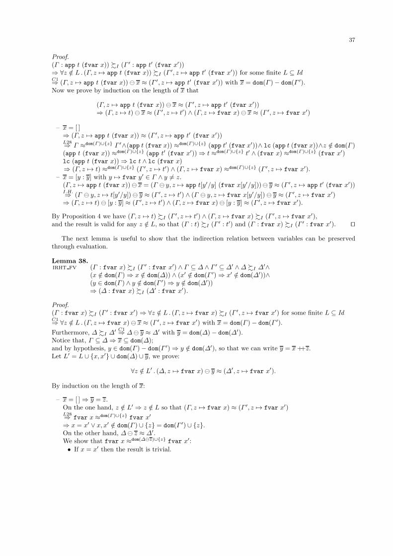
37
Proof.(Γ : app t (fvar x)) %I (Γ ′ : app t′ (fvar x′))⇒ ∀z /∈ L . (Γ, z 7→ app t (fvar x)) %I (Γ ′, z 7→ app t′ (fvar x′)) for some finite L ⊆ IdC1⇒ (Γ, z 7→ app t (fvar x))⊖ x ≈ (Γ ′, z 7→ app t′ (fvar x′)) with x = dom(Γ )− dom(Γ ′).Now we prove by induction on the length of x that
(Γ, z 7→ app t (fvar x))⊖ x ≈ (Γ ′, z 7→ app t′ (fvar x′))⇒ (Γ, z 7→ t)⊖ x ≈ (Γ ′, z 7→ t′) ∧ (Γ, z 7→ fvar x)⊖ x ≈ (Γ ′, z 7→ fvar x′)
– x = [ ]⇒ (Γ, z 7→ app t (fvar x)) ≈ (Γ ′, z 7→ app t′ (fvar x′))L28⇒ Γ ≈dom(Γ )∪{z} Γ ′∧(app t (fvar x)) ≈dom(Γ )∪{z} (app t′ (fvar x′))∧ lc (app t (fvar x))∧z /∈ dom(Γ )(app t (fvar x)) ≈dom(Γ )∪{z} (app t′ (fvar x′))⇒ t ≈dom(Γ )∪{z} t′ ∧ (fvar x) ≈dom(Γ )∪{z} (fvar x′)lc (app t (fvar x))⇒ lc t ∧ lc (fvar x)⇒ (Γ, z 7→ t) ≈dom(Γ )∪{z} (Γ ′, z 7→ t′) ∧ (Γ, z 7→ fvar x) ≈dom(Γ )∪{z} (Γ ′, z 7→ fvar x′).
– x = [y : y] with y 7→ fvar y′ ∈ Γ ∧ y 6= z.(Γ, z 7→ app t (fvar x))⊖ x = (Γ ⊖ y, z 7→ app t[y′/y] (fvar x[y′/y]))⊖ y ≈ (Γ ′, z 7→ app t′ (fvar x′))I.H.⇒ (Γ ⊖ y, z 7→ t[y′/y])⊖ y ≈ (Γ ′, z 7→ t′) ∧ (Γ ⊖ y, z 7→ fvar x[y′/y])⊖ y ≈ (Γ ′, z 7→ fvar x′)⇒ (Γ, z 7→ t)⊖ [y : y] ≈ (Γ ′, z 7→ t′) ∧ (Γ, z 7→ fvar x)⊖ [y : y] ≈ (Γ ′, z 7→ fvar x′).
By Proposition 4 we have (Γ, z 7→ t) %I (Γ ′, z 7→ t′) ∧ (Γ, z 7→ fvar x) %I (Γ ′, z 7→ fvar x′),and the result is valid for any z /∈ L, so that (Γ : t) %I (Γ ′ : t′) and (Γ : fvar x) %I (Γ ′ : fvar x′). ⊓⊔
The next lemma is useful to show that the indirection relation between variables can be preservedthrough evaluation.
Lemma 38.irht fv (Γ : fvar x) %I (Γ ′ : fvar x′) ∧ Γ ⊆ ∆ ∧ Γ ′ ⊆ ∆′ ∧∆ %I ∆′∧
(x /∈ dom(Γ )⇒ x /∈ dom(∆)) ∧ (x′ /∈ dom(Γ ′)⇒ x′ /∈ dom(∆′))∧(y ∈ dom(Γ ) ∧ y /∈ dom(Γ ′)⇒ y /∈ dom(∆′))⇒ (∆ : fvar x) %I (∆′ : fvar x′).
Proof.(Γ : fvar x) %I (Γ ′ : fvar x′)⇒ ∀z /∈ L . (Γ, z 7→ fvar x) %I (Γ ′, z 7→ fvar x′) for some finite L ⊆ IdC1⇒ ∀z /∈ L . (Γ, z 7→ fvar x)⊖ x ≈ (Γ ′, z 7→ fvar x′) with x = dom(Γ )− dom(Γ ′).
Furthermore, ∆ %I ∆′ C1⇒ ∆⊖ y ≈ ∆′ with y = dom(∆)− dom(∆′).Notice that, Γ ⊆ ∆⇒ x ⊆ dom(∆);and by hypothesis, y ∈ dom(Γ )− dom(Γ ′)⇒ y /∈ dom(∆′), so that we can write y = x ++z.Let L′ = L ∪ {x, x′} ∪ dom(∆) ∪ y, we prove:
∀z /∈ L′ . (∆, z 7→ fvar x)⊖ y ≈ (∆′, z 7→ fvar x′).
By induction on the length of x:
– x = [ ]⇒ y = z.On the one hand, z /∈ L′ ⇒ z /∈ L so that (Γ, z 7→ fvar x) ≈ (Γ ′, z 7→ fvar x′)L28⇒ fvar x ≈dom(Γ )∪{z} fvar x′
⇒ x = x′ ∨ x, x′ /∈ dom(Γ ) ∪ {z} = dom(Γ ′) ∪ {z}.On the other hand, ∆⊖ z ≈ ∆′.We show that fvar x ≈dom(∆⊖z)∪{z} fvar x′:• If x = x′ then the result is trivial.
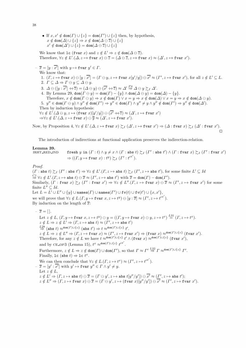
38
• If x, x′ /∈ dom(Γ ) ∪ {z} = dom(Γ ′) ∪ {z} then, by hypothesis,x /∈ dom(∆) ∪ {z} ⇒ x /∈ dom(∆⊖ z) ∪ {z}x′ /∈ dom(∆′) ∪ {z} = dom(∆⊖ z) ∪ {z}
We know that lc (fvar x) and z /∈ L′ ⇒ z /∈ dom(∆⊖ z).Therefore, ∀z /∈ L′.(∆, z 7→ fvar x)⊖ z = (∆⊖ z, z 7→ fvar x) ≈ (∆′, z 7→ fvar x′).
– x = [y : x′] with y 7→ fvar y′ ∈ Γ .We know that:1. (Γ, z 7→ fvar x)⊖ [y : x′] = (Γ ⊖ y, z 7→ fvar x[y′/y])⊖ x′ ≈ (Γ ′, z 7→ fvar x′), for all z /∈ L′ ⊆ L.2. Γ ⊆ ∆⇒ Γ ⊖ y ⊆ ∆⊖ y.
3. ∆⊖ ([y : x′] ++z) = (∆⊖ y)⊖ (x′ ++z) ≈ ∆′ P4⇒ ∆⊖ y %I ∆′.4. By Lemma 29, dom(Γ ⊖ y) = dom(Γ )− {y} ∧ dom(∆⊖ y) = dom(∆)− {y}.
Therefore, x /∈ dom(Γ ⊖ y)⇒ x /∈ dom(Γ ) ∨ x = y ⇒ x /∈ dom(∆) ∨ x = y ⇒ x /∈ dom(∆⊖ y).5. y′′ ∈ dom(Γ ⊖ y) ∧ y′′ /∈ dom(Γ ′)⇒ y′′ ∈ dom(Γ ) ∧ y′′ 6= y ∧ y′′ /∈ dom(Γ ′)⇒ y′′ /∈ dom(∆′).
Then by induction hypothesis:∀z /∈ L′.(∆⊖ y, z 7→ (fvar x)[y′/y])⊖ (x′ ++z) ≈ (∆′, z 7→ fvar x′)⇒∀z /∈ L′.(∆, z 7→ fvar x)⊖ y ≈ (∆′, z 7→ fvar x′).
Now, by Proposition 4, ∀z /∈ L′.(∆, z 7→ fvar x) %I (∆′, z 7→ fvar x′)⇒ (∆ : fvar x) %I (∆′ : fvar x′).⊓⊔
The introduction of indirections at functional application preserves the indirection-relation.
Lemma 39.irht red ind fresh y in (Γ : t) ∧ y 6= x ∧ (Γ : abs t) %I (Γ ′ : abs t′) ∧ (Γ : fvar x) %I (Γ ′ : fvar x′)
⇒ ((Γ, y 7→ fvar x) : ty) %I (Γ ′ : t′x′).
Proof.(Γ : abs t) %I (Γ ′ : abs t′)⇒ ∀z /∈ L′.(Γ, z 7→ abs t) %I (Γ ′, z 7→ abs t′), for some finite L′ ⊆ IdC1⇒ ∀z /∈ L′.(Γ, z 7→ abs t)⊖ x ≈ (Γ ′, z 7→ abs t′) with x = dom(Γ )− dom(Γ ′).Similarly, (Γ : fvar x) %I (Γ ′ : fvar x′) ⇒ ∀z /∈ L′′.(Γ, z 7→ fvar x) ⊖ x ≈ (Γ ′, z 7→ fvar x′) for somefinite L′′ ⊆ Id .Let L = L′ ∪ L′′ ∪ {y} ∪ names(Γ ) ∪ names(Γ ′) ∪ fv(t) ∪ fv(t′) ∪ {x, x′},we will prove that ∀z /∈ L.(Γ, y 7→ fvar x, z 7→ ty)⊖ [y : x] ≈ (Γ ′, z 7→ t′x
′).
By induction on the length of x:
– x = [ ].
Let z /∈ L, (Γ, y 7→ fvar x, z 7→ ty)⊖ y = ((Γ, y 7→ fvar x) ⊖ y, z 7→ tx)L31= (Γ, z 7→ tx).
z /∈ L⇒ z /∈ L′ ⇒ (Γ, z 7→ abs t) ≈ (Γ ′, z 7→ abs t′)L28⇒ (abs t) ≈dom(Γ )∪{z} (abs t′)⇒ t ≈dom(Γ )∪{z} t′.z /∈ L⇒ z /∈ L′′ ⇒ (Γ, z 7→ fvar x) ≈ (Γ ′, z 7→ fvar x′)⇒ (fvar x) ≈dom(Γ )∪{z} (fvar x′).Therefore, for any z /∈ L we have t ≈dom(Γ )∪{z} t′ ∧ (fvar x) ≈dom(Γ )∪{z} (fvar x′),
and by ce op3 (Lemma 15), tx ≈dom(Γ )∪{z} t′x′.
Furthermore, z /∈ L⇒ z /∈ dom(Γ ) ∪ dom(Γ ′), so that Γ ≈ Γ ′ L32⇒ Γ ≈dom(Γ )∪{z} Γ ′.Finally, lc (abs t)⇒ lc tx.
We can then conclude that ∀z /∈ L.(Γ, z 7→ tx) ≈ (Γ ′, z 7→ t′x′).
– x = [y′ : x′] with y′ 7→ fvar y′′ ∈ Γ ∧ y′ 6= y.Let z /∈ L,z /∈ L′ ⇒ (Γ, z 7→ abs t)⊖ x = (Γ ⊖ y′, z 7→ abs t[y′′/y′])⊖ x′ ≈ (Γ ′, z 7→ abs t′);z /∈ L′′ ⇒ (Γ, z 7→ fvar x)⊖ x = (Γ ⊖ y′, z 7→ (fvar x)[y′′/y′])⊖ x′ ≈ (Γ ′, z 7→ fvar x′).

39
By induction hypothesis:
(Γ ⊖ y′, y 7→ (fvar x)[y′′/y′], z 7→ t[y′′/y′]y)⊖ [y : x′] ≈ (Γ ′, z 7→ t′x′)
y 6=y′⇒ (Γ, y 7→ fvar x, z 7→ ty)⊖ [y′ : y : x′] ≈ (Γ ′, z 7→ t′x
′)
L19⇒ (Γ, y 7→ fvar x, z 7→ ty)⊖ [y : y′ : x′] ≈ (Γ ′, z 7→ t′x′)
⇒ (Γ, y 7→ fvar x, z 7→ ty)⊖ [y : x] ≈ (Γ ′, z 7→ t′x′).
Now we check that ok (Γ, y 7→ fvar x, z 7→ ty):
Γ %I Γ ′′ L20⇒ ok Γ ∧ ok Γ ′
y /∈ dom(Γ )lc (fvar x)
⇒ ok (Γ, y 7→ fvar x).
ok (Γ, y 7→ fvar x)z /∈ L ⊇ dom(Γ ) ∪ {y}lc (abs t)⇒ lc ty
⇒ ok (Γ, y 7→ fvar x, z 7→ ty).
By Proposition 4,
∀z /∈ L.(Γ, y 7→ fvar x, z 7→ ty)⊖ [y : x] ≈ (Γ ′, z 7→ t′x′)⇒ ((Γ, y 7→ fvar x) : ty) %I (Γ ′ : t′x
′). ⊓⊔
If two let expressions are indirection related, then their body terms are also related with respect to theheaps extended with the local declarations.
Lemma 40.intr vars fresh x in (Γ : let t in t) ∧ fresh x in (Γ ′ : let t′ in t′)∧
(Γ : let t in t) %I (Γ ′ : let t′ in t′)⇒ ((Γ, x 7→ tx) : tx) %I ((Γ ′, x 7→ t′
x) : t′x).
Proof.(Γ : let t in t) %I (Γ ′ : let t′ in t′)⇒ ∀z /∈ L . (Γ, z 7→ let t in t) %I (Γ ′, z 7→ let t′ in t′) for some finite L ⊆ IdC1⇒ (Γ, z 7→ let t in t)⊖ y ≈ (Γ ′, z 7→ let t′ in t′) with y = dom(Γ )− dom(Γ ′).Consider any z /∈ L such that fresh z in (Γ : let t in t) ∧ fresh z in (Γ ′ : let t′ in t′) ∧ z /∈ x.Now we prove by induction on the length of y that
(Γ, z 7→ let t in t)⊖ y ≈ (Γ ′, z 7→ let t′ in t′)⇒ (Γ, x 7→ tx, z 7→ tx)⊖ y ≈ (Γ ′, x 7→ t′
x, z 7→ t′x)
– y = [ ]⇒ (Γ, z 7→ let t in t) ≈ (Γ ′, z 7→ let t′ in t′)L28⇒ Γ ≈dom(Γ )∪{z} Γ ′ ∧ let t in t ≈dom(Γ )∪{z} let t′ in t′ ∧ lc (let t′ in t′) ∧ z /∈ dom(Γ )let t in t ≈dom(Γ )∪{z} let t′ in t′ ⇒ |t| = |t′| ∧ t ≈dom(Γ )∪{z} t′ ∧ t ≈dom(Γ )∪{z} t′
L14⇒ t ≈dom(Γ )∪x∪{z} t′ ∧ t ≈dom(Γ )∪x∪{z} t′L15⇒ t
x ≈dom(Γ )∪x∪{z} t′x ∧ tx ≈dom(Γ )∪x∪{z} t′x.
lc let t′ in t′ ⇒ lc tx ∧ lc tx ⇒ ok (Γ, x 7→ t
x, z 7→ tx) ∧ ok (Γ ′, x 7→ t′
x, z 7→ t′x)
L17⇒ (Γ, x 7→ tx, z 7→ tx) ≈ (Γ ′, x 7→ t′
x, z 7→ t′x).
– y = [y : z] with y 7→ fvar y′ ∈ Γ ∧ y 6= z.fresh x in (Γ : let t in t)⇒ fresh x in Γ ⊖ y : let t[y′/y] in t[y′/y].(Γ, z 7→ let t in t)⊖ y = (Γ ⊖ y, z 7→ let t[y′/y] in t[y′/y])⊖ z ≈ (Γ ′, z 7→ let t′ in t′).I.H.⇒ (Γ ⊖ y, x 7→ t[y′/y]x, z 7→ t[y′/y]x)⊖ z ≈ (Γ ′, x 7→ t′
x, z 7→ t′x)
⇒ (Γ, x 7→ tx, z 7→ tx)⊖ y ≈ (Γ ′, x 7→ t′
x, z 7→ t′x).
By Proposition 4 we have (Γ, x 7→ tx, z 7→ tx) %I (Γ ′, x 7→ t′
x, z 7→ t′x) and the result is valid for any
z /∈ L and sufficiently fresh, so that ((Γ, x 7→ tx) : tx) %I ((Γ ′, x 7→ t′
x) : t′x). ⊓⊔
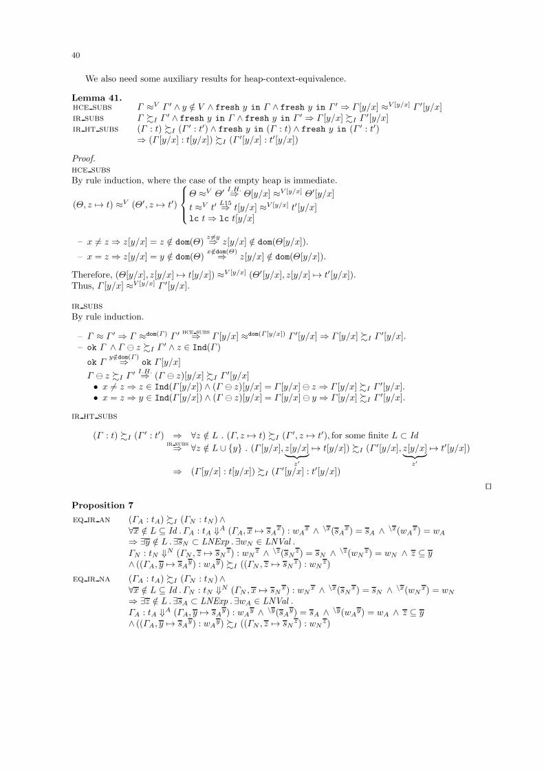
40
We also need some auxiliary results for heap-context-equivalence.
Lemma 41.hce subs Γ ≈V Γ ′ ∧ y /∈ V ∧ fresh y in Γ ∧ fresh y in Γ ′ ⇒ Γ [y/x] ≈V [y/x] Γ ′[y/x]ir subs Γ %I Γ ′ ∧ fresh y in Γ ∧ fresh y in Γ ′ ⇒ Γ [y/x] %I Γ ′[y/x]ir ht subs (Γ : t) %I (Γ ′ : t′) ∧ fresh y in (Γ : t) ∧ fresh y in (Γ ′ : t′)
⇒ (Γ [y/x] : t[y/x]) %I (Γ ′[y/x] : t′[y/x])
Proof.hce subsBy rule induction, where the case of the empty heap is immediate.
(Θ, z 7→ t) ≈V (Θ′, z 7→ t′)
Θ ≈V Θ′ I.H.⇒ Θ[y/x] ≈V [y/x] Θ′[y/x]
t ≈V t′L15⇒ t[y/x] ≈V [y/x] t′[y/x]
lc t⇒ lc t[y/x]
– x 6= z ⇒ z[y/x] = z /∈ dom(Θ)z 6=y⇒ z[y/x] /∈ dom(Θ[y/x]).
– x = z ⇒ z[y/x] = y /∈ dom(Θ)x/∈dom(Θ)⇒ z[y/x] /∈ dom(Θ[y/x]).
Therefore, (Θ[y/x], z[y/x] 7→ t[y/x]) ≈V [y/x] (Θ′[y/x], z[y/x] 7→ t′[y/x]).Thus, Γ [y/x] ≈V [y/x] Γ ′[y/x].
ir subsBy rule induction.
– Γ ≈ Γ ′ ⇒ Γ ≈dom(Γ ) Γ ′ hce subs⇒ Γ [y/x] ≈dom(Γ [y/x]) Γ ′[y/x]⇒ Γ [y/x] %I Γ ′[y/x].– ok Γ ∧ Γ ⊖ z %I Γ ′ ∧ z ∈ Ind(Γ )
ok Γy/∈dom(Γ )⇒ ok Γ [y/x]
Γ ⊖ z %I Γ ′ I.H.⇒ (Γ ⊖ z)[y/x] %I Γ ′[y/x]• x 6= z ⇒ z ∈ Ind(Γ [y/x]) ∧ (Γ ⊖ z)[y/x] = Γ [y/x]⊖ z ⇒ Γ [y/x] %I Γ ′[y/x].• x = z ⇒ y ∈ Ind(Γ [y/x]) ∧ (Γ ⊖ z)[y/x] = Γ [y/x]⊖ y ⇒ Γ [y/x] %I Γ ′[y/x].
ir ht subs
(Γ : t) %I (Γ ′ : t′) ⇒ ∀z /∈ L . (Γ, z 7→ t) %I (Γ ′, z 7→ t′), for some finite L ⊂ Idir subs⇒ ∀z /∈ L ∪ {y} . (Γ [y/x], z[y/x]︸ ︷︷ ︸
z′
7→ t[y/x]) %I (Γ ′[y/x], z[y/x]︸ ︷︷ ︸z′
7→ t′[y/x])
⇒ (Γ [y/x] : t[y/x]) %I (Γ ′[y/x] : t′[y/x])
⊓⊔
Proposition 7
eq ir an (ΓA : tA) %I (ΓN : tN )∧∀x /∈ L ⊆ Id . ΓA : tA ⇓A (ΓA, x 7→ sA
x) : wAx ∧ \x(sA
x) = sA ∧ \x(wAx) = wA
⇒ ∃y /∈ L . ∃sN ⊂ LNExp . ∃wN ∈ LNVal .
ΓN : tN ⇓N (ΓN , z 7→ sNz) : wN
z ∧ \z(sNz) = sN ∧ \z(wNz) = wN ∧ z ⊆ y
∧ ((ΓA, y 7→ sAy) : wA
y) %I ((ΓN , z 7→ sNz) : wN
z)
eq ir na (ΓA : tA) %I (ΓN : tN )∧∀x /∈ L ⊆ Id . ΓN : tN ⇓N (ΓN , x 7→ sN
x) : wNx ∧ \x(sN
x) = sN ∧ \x(wNx) = wN
⇒ ∃z /∈ L . ∃sA ⊂ LNExp . ∃wA ∈ LNVal .ΓA : tA ⇓A (ΓA, y 7→ sA
y) : wAy ∧ \y(sAy) = sA ∧ \y(wA
y) = wA ∧ z ⊆ y∧ ((ΓA, y 7→ sA
y) : wAy) %I ((ΓN , z 7→ sN
z) : wNz)

41
Proof.
(ΓA : tA) %I (ΓN : tN )L22⇒ tA ∼S tN .
eq ir an: By rule induction:
– Rule LNLamtA ≡ abs uA ⇒ tN ≡ abs uN , and in this case x = [ ] (so that y = [ ] too).It is easy to prove that for any t ∈ LNExp it is t[ ] = t = \[ ]t.(ΓA : abs uA) %I (ΓN : abs uN ) ⇒ ∀z /∈ L′ . (ΓA, z 7→ abs uA) %I (ΓN , z 7→ abs uN )
L20⇒ ok (ΓN , z 7→ abs uN )⇒ ok ΓN ∧ lc (abs uN)
LNLam⇒ ΓN : abs uN ⇓N ΓN : abs uN , and take z = [ ].
– Rule ALNVar.tA ≡ fvar xA ∧ ΓA = (Γ ′
A, xA 7→ uA).On the one hand, ∀x /∈ L.(Γ ′
A, xA 7→ uA) : fvar xA ⇓A (ΓA, x 7→ sAx) : wA
x
⇒ ∀x /∈ L.(Γ ′A, xA 7→ uA) : uA ⇓A (ΓA, x 7→ sA
x) : wAx.
On the other hand, tN ≡ fvar xN and, by hypothesis, ((Γ ′A, xA 7→ uA) : fvar xA) %I (ΓN : fvar xN )
L34⇒ ΓN = (Γ ′N , xN 7→ uN )
L36⇒ ((Γ ′A, xA 7→ uA) : uA) %I ((Γ ′
N , xN 7→ uN) : uN)∨((Γ ′
A, xA 7→ uA) : uA) %I ((Γ ′N , xN 7→ uN) : fvar xN ).
In the first case, by induction hypothesis we have (Γ ′N , xN 7→ uN ) : uN ⇓N (ΓN , z 7→ sN
z) : wNz
and ((ΓA, y 7→ sAy) : wA
y) %I ((ΓN , z 7→ sNz) : wN
z), for some z ⊆ y /∈ L, sN and wN .By applying rule ALNVar to this result we obtain ΓN : tN ⇓N (ΓN , z 7→ sN
z) : wNz.
In the second case, by induction hypothesis we obtain directly(Γ ′
N , xN 7→ uN) : fvar xN ⇓N (ΓN , z 7→ sNz) : wN
z ,with ((ΓA, y 7→ sA
y) : wAy) %I ((ΓN , z 7→ sN
z) : wNz) for some z ⊆ y /∈ L, sN and wN .
– Rule ALNApp.tA ≡ app t′A (fvar xA)⇒ tN ≡ app t′N (fvar xN ).By hypothesis, ∀x /∈ L . ΓA : app t′A (fvar xA) ⇓A (ΓA, x 7→ sA
x) : wAx.
Let us choose a particular x /∈ L such that fresh x in (ΓA : tA);x can be decomposed as x = [z : x1 ++x2] with
ΓA : t′A ⇓A (ΓA, x1 7→ s1Ax1) : abs u′
Ax1 (3)
and
(ΓA, x1 7→ s1Ax1 , z 7→ fvar xA) : (u′
Ax1)z ⇓A (ΓA, x1 7→ s1A
x1 , z 7→ fvar xA, x2 7→ s2Ax2) : w′
Az
(4)
where w′Az
= wAx.
Let L′ = L ∪ names(ΓA : tA) ∪ fv(s1A) ∪ fv(u′A) ∪ {xN}; by applying renaming2 (Lemma 12) to (3)
we obtain∀x1 /∈ L′ . ΓA : t′A ⇓A (ΓA, x1 7→ s1A
x1) : abs u′Ax1 .
By hypothesis, (ΓA : app t′A (fvar xA)) %I (ΓN : app t′N (fvar xN ))L37⇒ (ΓA : t′A) %I (ΓN : t′N ), so
that by induction hypothesis
ΓN : t′N ⇓N (ΓN , z1 7→ s1Nz1) : w′
Nz1 ∧ ((ΓA, y1 7→ s1A
y1) : abs u′Ay1) %I ((ΓN , z1 7→ s1N
z1) : w′N
z1)
for some y1 /∈ L′, and with z1 ⊆ y1. It must be that w′N
z1 ≡ abs uN for some term uN .Now we apply renaming1 (Lemma 12) to (4) to obtain
(ΓA, y1 7→ s1Ay1 , z 7→ fvar xA) : (u′
Ay1)z ⇓A (ΓA, y1 7→ s1A
y1 , z 7→ fvar xA, x2 7→ s2Ax2) : w′′
Az
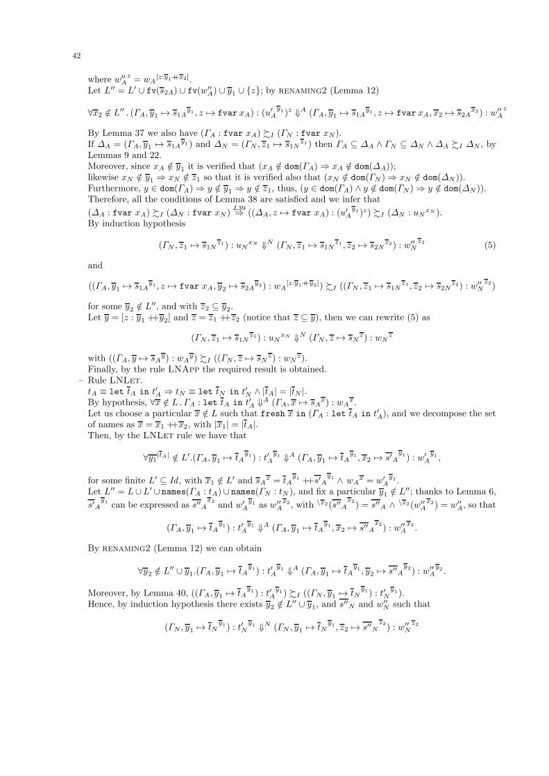
42
where w′′Az
= wA[z:y1++x2].
Let L′′ = L′ ∪ fv(s2A) ∪ fv(w′′A) ∪ y1 ∪ {z}; by renaming2 (Lemma 12)
∀x2 /∈ L′′ . (ΓA, y1 7→ s1Ay1 , z 7→ fvar xA) : (u′
Ay1)z ⇓A (ΓA, y1 7→ s1A
y1 , z 7→ fvar xA, x2 7→ s2Ax2) : w′′
Az
By Lemma 37 we also have (ΓA : fvar xA) %I (ΓN : fvar xN ).If ∆A = (ΓA, y1 7→ s1A
y1) and ∆N = (ΓN , z1 7→ s1Nz1) then ΓA ⊆ ∆A ∧ ΓN ⊆ ∆N ∧∆A %I ∆N , by
Lemmas 9 and 22.Moreover, since xA /∈ y1 it is verified that (xA /∈ dom(ΓA)⇒ xA /∈ dom(∆A));likewise xN /∈ y1 ⇒ xN /∈ z1 so that it is verified also that (xN /∈ dom(ΓN )⇒ xN /∈ dom(∆N )).Furthermore, y ∈ dom(ΓA)⇒ y /∈ y1 ⇒ y /∈ z1, thus, (y ∈ dom(ΓA) ∧ y /∈ dom(ΓN )⇒ y /∈ dom(∆N )).Therefore, all the conditions of Lemma 38 are satisfied and we infer that
(∆A : fvar xA) %I (∆N : fvar xN )L39⇒ ((∆A, z 7→ fvar xA) : (u′
Ay1)z) %I (∆N : uN
xN ).By induction hypothesis
(ΓN , z1 7→ s1Nz1) : uN
xN ⇓N (ΓN , z1 7→ s1Nz1 , z2 7→ s2N
z2) : w′′N
z2 (5)
and
((ΓA, y1 7→ s1Ay1 , z 7→ fvar xA, y2 7→ s2A
y2) : wA[z:y1++y2]) %I ((ΓN , z1 7→ s1N
z1 , z2 7→ s2Nz2) : w′′
Nz2)
for some y2 /∈ L′′, and with z2 ⊆ y2.Let y = [z : y1 ++y2] and z = z1 ++z2 (notice that z ⊆ y), then we can rewrite (5) as
(ΓN , z1 7→ s1Nz1) : uN
xN ⇓N (ΓN , z 7→ sNz) : wN
z
with ((ΓA, y 7→ sAy) : wA
y) %I ((ΓN , z 7→ sNz) : wN
z).Finally, by the rule LNApp the required result is obtained.
– Rule LNLet.tA ≡ let tA in t′A ⇒ tN ≡ let tN in t′N ∧ |tA| = |tN |.By hypothesis, ∀x /∈ L . ΓA : let tA in t′A ⇓A (ΓA, x 7→ sA
x) : wAx.
Let us choose a particular x /∈ L such that fresh x in (ΓA : let tA in t′A), and we decompose the setof names as x = x1 ++x2, with |x1| = |tA|.Then, by the LNLet rule we have that
∀y1|tA| /∈ L′.(ΓA, y1 7→ tA
y1) : t′Ay1 ⇓A (ΓA, y1 7→ tA
y1 , x2 7→ s′Ay1) : w′
Ay1 ,
for some finite L′ ⊆ Id , with x1 /∈ L′ and sAx = tA
y1 ++s′Ay1 ∧ wA
x = w′Ay1 .
Let L′′ = L∪L′ ∪ names(ΓA : tA)∪ names(ΓN : tN ), and fix a particular y1 /∈ L′′; thanks to Lemma 6,
s′Ay1 can be expressed as s′′A
x2and w′
Ay1 as w′′
Ax2 , with \x2(s′′A
x2) = s′′A ∧ \x2(w′′
Ax2) = w′′
A, so that
(ΓA, y1 7→ tAy1) : t′A
y1 ⇓A (ΓA, y1 7→ tAy1 , x2 7→ s′′A
x2) : w′′
Ax2 .
By renaming2 (Lemma 12) we can obtain
∀y2 /∈ L′′ ∪ y1.(ΓA, y1 7→ tAy1) : t′A
y1 ⇓A (ΓA, y1 7→ tAy1 , y2 7→ s′′A
y2) : w′′Ay2 .
Moreover, by Lemma 40, ((ΓA, y1 7→ tAy1) : t′A
y1) %I ((ΓN , y1 7→ tNy1) : t′N
y1).Hence, by induction hypothesis there exists y2 /∈ L′′ ∪ y1, and s′′N and w′′
N such that
(ΓN , y1 7→ tNy1) : t′N
y1 ⇓N (ΓN , y1 7→ tNy1 , z2 7→ s′′N
z2) : w′′
Nz2

43
with \z2(s′′Nz2
) = s′′N ∧ \z2(w′′N
z2) = w′′N ∧ z2 ⊆ y2,
and (ΓA, y1 7→ tAy1 , y2 7→ s′′A
y2) : w′′Ay2) %I ((ΓN , y1 7→ tN
y1 , z2 7→ s′′Nz2
) : w′′N
z2).Notice that y1 ++y2 /∈ L.
By Lemma 6, tNy1 ++s′′N
z2can be expressed as s′N
y1 and w′′N
z2 as w′N
y1 with \y1(s′Ny1) = s′N ∧
\y1(w′N
y1) = w′N .
Let L′′′ = L′′ ∪ fv(sA) ∪ fv(wA) ∪ fv(s′N ) ∪ fv(w′N ) ∪ y1 ++y2 ∪ z2;
by renaming1 (Lemma 12) we obtain
∀z1 /∈ L′′′.(ΓN , z1 7→ tNz1) : t′N
z1 ⇓N (ΓN , z1 ++z2 7→ s′Nz1
) : w′N
z1 .
Then, by the LNLet rule we infer that
ΓN : let tN in t′N ⇓N (ΓN , z1 ++z2 7→ s′Nz1
) : w′N
z1 , for some z1 /∈ L′′′.
Once again, by Lemma 6, we rewrite s′Nz1
= sNz1++z2 and w′
Nz1 = wN
z1++z2 .
Besides, notice that tAy1 ++s′′A
y2 = sAz1++y2 and w′′
Ay2 = wA
y1++y2 ; hence((ΓA, y1 ++y2 7→ sA
y1++y2) : wAy1++y2) %I ((ΓN , y1 ++z2 7→ sN
y1++z2) : wNy1++z2)
L41⇒ (ΓA, z1 ++y2 7→ sAz1++y2) : wA
z1++y2) %I ((ΓN , z1 ++z2 7→ sNz1++z2) : wN
z1++z2),and notice that z1 ++z2 ⊆ z1 ++y2 /∈ L.
eq ir na: By rule induction.For rules LNLam and LNLet we follow similar reasonings as in eq ir an. Therefore, we detail only thecases of rules ALNVar and LNApp:
– Rule ALNVar.tN ≡ fvar xN ∧ ΓN = (Γ ′
N , xN 7→ uN).On the one hand, ∀x /∈ L.(Γ ′
N , xN 7→ uN ) : fvar xN ⇓N (ΓN , x 7→ sNx) : wN
x
⇒ ∀x /∈ L.(Γ ′N , xN 7→ uN ) : uN ⇓N (ΓN , x 7→ sN
x) : wNx.
On the other hand, tA ≡ fvar xA and, by hypothesis, (ΓA : fvar xA) %I ((Γ ′N , xN 7→ uN ) : fvar xN )
L34⇒ ΓA = (Γ ′A, xA 7→ uA)∧
∃x0, . . . , xn ∈ Id . x0 = xA ∧ xn = xN ∧ ∀i : 0 ≤ i < n . xi 7→ fvar xi+1 ∈ (Γ ′A, xA 7→ uA).
Now we proceed by induction on n to prove that (Γ ′A, xA 7→ uA) : uA ⇓A (ΓA, y 7→ sA
y) : wAy
and ((ΓA, y 7→ sAy) : wA
y) %I ((ΓN , z 7→ sNz) : wN
z) for some z ⊆ y /∈ L.By applying rule ALNVar to this result we obtain ΓA : tA ⇓A (ΓA, y 7→ sA
y) : wAy.
• n = 0⇒ xA = xN
⇒ ((Γ ′A, xA 7→ uA) : fvar xA) %I ((Γ ′
N , xN 7→ uN ) : fvar xA)L22⇒ (Γ ′
A, xA 7→ uA) %I (Γ ′N , xN 7→ uN )
L35⇒ ((Γ ′A, xA 7→ uA) : uA) %I ((Γ ′
N , xN 7→ uN) : uN).By (rule) induction hypothesis we are done.• n > 0⇒ ((Γ ′
A, xA 7→ fvar x1) : fvar xA) %I ((Γ ′N , xN 7→ uN ) : fvar xN )
L36⇒ ((Γ ′A, xA 7→ fvar x1) : fvar x1) %I ((Γ ′
N , xN 7→ uN ) : uN)∨((Γ ′
A, xA 7→ fvar x1) : fvar x1) %I ((Γ ′N , xN 7→ uN ) : fvar xN ).
In the first case, by (rule) induction hypothesis we are done.In the second case, by Lemma 34, we have x1 ∈ dom(ΓA), so that ΓA = (Γ ′′
A, x1 7→ u1).Since the path from x1 to xN is of length n−1, the induction hypothesis indicates that there existsz ⊆ y /∈ L, such that(Γ ′′
A, x1 7→ u1) : u1 ⇓A (ΓA, y 7→ sAy) : wA
y and ((ΓA, y 7→ sAy) : wA
y) %I ((ΓN , z 7→ sNz) : wN
z).By applying rule ALNVar, we obtain (Γ ′′
A, x1 7→ u1) : fvar x1 ⇓A (ΓA, y 7→ sAy) : wA
y, i.e.,(Γ ′
A, xA 7→ fvar x1) : fvar x1 ⇓A (ΓA, y 7→ sAy) : wA
y.
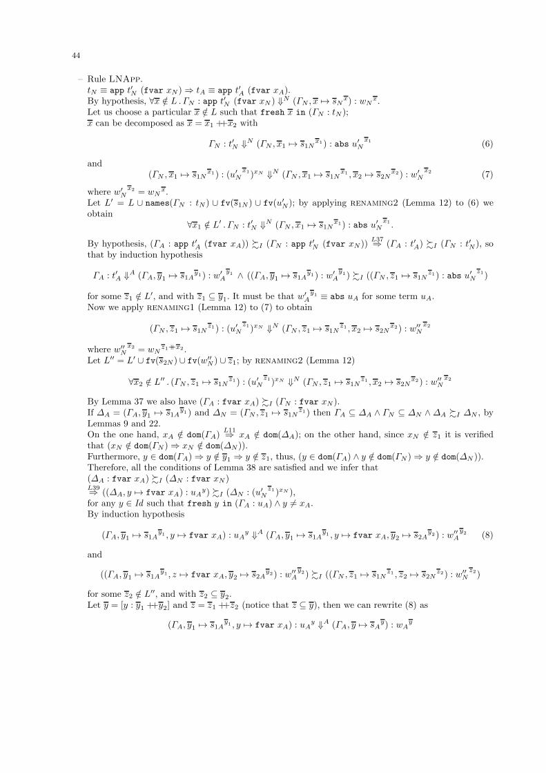
44
– Rule LNApp.tN ≡ app t′N (fvar xN )⇒ tA ≡ app t′A (fvar xA).By hypothesis, ∀x /∈ L . ΓN : app t′N (fvar xN ) ⇓N (ΓN , x 7→ sN
x) : wNx.
Let us choose a particular x /∈ L such that fresh x in (ΓN : tN );x can be decomposed as x = x1 ++x2 with
ΓN : t′N ⇓N (ΓN , x1 7→ s1Nx1) : abs u′
Nx1 (6)
and(ΓN , x1 7→ s1N
x1) : (u′N
x1)xN ⇓N (ΓN , x1 7→ s1Nx1 , x2 7→ s2N
x2) : w′N
x2 (7)
where w′N
x2 = wNx.
Let L′ = L ∪ names(ΓN : tN ) ∪ fv(s1N ) ∪ fv(u′N); by applying renaming2 (Lemma 12) to (6) we
obtain∀x1 /∈ L′ . ΓN : t′N ⇓N (ΓN , x1 7→ s1N
x1) : abs u′N
x1 .
By hypothesis, (ΓA : app t′A (fvar xA)) %I (ΓN : app t′N (fvar xN ))L37⇒ (ΓA : t′A) %I (ΓN : t′N ), so
that by induction hypothesis
ΓA : t′A ⇓A (ΓA, y1 7→ s1Ay1) : w′
Ay1 ∧ ((ΓA, y1 7→ s1A
y1) : w′Ay1) %I ((ΓN , z1 7→ s1N
z1) : abs u′N
z1)
for some z1 /∈ L′, and with z1 ⊆ y1. It must be that w′Ay1 ≡ abs uA for some term uA.
Now we apply renaming1 (Lemma 12) to (7) to obtain
(ΓN , z1 7→ s1Nz1) : (u′
Nz1)xN ⇓N (ΓN , z1 7→ s1N
z1 , x2 7→ s2Nx2) : w′′
Nx2
where w′′N
x2 = wNz1++x2 .
Let L′′ = L′ ∪ fv(s2N ) ∪ fv(w′′N ) ∪ z1; by renaming2 (Lemma 12)
∀x2 /∈ L′′ . (ΓN , z1 7→ s1Nz1) : (u′
Nz1)xN ⇓N (ΓN , z1 7→ s1N
z1 , x2 7→ s2Nx2) : w′′
Nx2
By Lemma 37 we also have (ΓA : fvar xA) %I (ΓN : fvar xN ).If ∆A = (ΓA, y1 7→ s1A
y1) and ∆N = (ΓN , z1 7→ s1Nz1) then ΓA ⊆ ∆A ∧ ΓN ⊆ ∆N ∧∆A %I ∆N , by
Lemmas 9 and 22.On the one hand, xA /∈ dom(ΓA)
L11⇒ xA /∈ dom(∆A); on the other hand, since xN /∈ z1 it is verifiedthat (xN /∈ dom(ΓN )⇒ xN /∈ dom(∆N )).Furthermore, y ∈ dom(ΓA)⇒ y /∈ y1 ⇒ y /∈ z1, thus, (y ∈ dom(ΓA) ∧ y /∈ dom(ΓN )⇒ y /∈ dom(∆N )).Therefore, all the conditions of Lemma 38 are satisfied and we infer that(∆A : fvar xA) %I (∆N : fvar xN )L39⇒ ((∆A, y 7→ fvar xA) : uA
y) %I (∆N : (u′N
z1)xN ),for any y ∈ Id such that fresh y in (ΓA : uA) ∧ y 6= xA.By induction hypothesis
(ΓA, y1 7→ s1Ay1 , y 7→ fvar xA) : uA
y ⇓A (ΓA, y1 7→ s1Ay1 , y 7→ fvar xA, y2 7→ s2A
y2) : w′′Ay2 (8)
and
((ΓA, y1 7→ s1Ay1 , z 7→ fvar xA, y2 7→ s2A
y2) : w′′Ay2) %I ((ΓN , z1 7→ s1N
z1 , z2 7→ s2Nz2) : w′′
Nz2)
for some z2 /∈ L′′, and with z2 ⊆ y2.Let y = [y : y1 ++y2] and z = z1 ++z2 (notice that z ⊆ y), then we can rewrite (8) as
(ΓA, y1 7→ s1Ay1 , y 7→ fvar xA) : uA
y ⇓A (ΓA, y 7→ sAy) : wA
y

45
with ((ΓA, y 7→ sAy) : wA
y) %I ((ΓN , z 7→ sNz) : wN
z).Finally, let L′′′ = names(ΓA)∪fv(sA)∪fv(uA)∪fv(wA)∪{xA}∪y, we apply renaming1 (Lemma 12)to (8) to obtain
∀y /∈ L′′′ . (ΓA, y1 7→ s1Ay1 , y 7→ fvar xA) : uA
y ⇓A (ΓA, y 7→ sAy) : wA
y
so that the required result is obtained by the rule ALNApp.⊓⊔
Lemma 42.irht ref ok Γ ∧ lc t⇒ (Γ : t) %I (Γ : t)
Proof.
ok Γ ∧ lc t⇒ ∀z /∈ dom(Γ ) . ok (Γ, z 7→ t)P5⇒ ∀z /∈ dom(Γ ) . (Γ, z 7→ t) %I (Γ, z 7→ t)⇒ (Γ : t) %I (Γ : t).
⊓⊔
Theorem 1 (Equivalence)
eq an Γ : t ⇓A ∆A : wA ⇒∃∆N ∈ LNHeap . ∃wN ∈ LNVal . Γ : t ⇓N ∆N : wN ∧ (∆A : wA) %I (∆N : wN )
eq na Γ : t ⇓N ∆N : wN ⇒∃∆A ∈ LNHeap . ∃wA ∈ LNVal . ∃x ⊆ dom(∆N )− dom(Γ ) . ∃y ⊆ Id . |x| = |y| ∧Γ : t ⇓A ∆A : wA ∧ (∆A : wA) %I (∆N [y/x] : wN [y/x])
Proof.eq anAssume Γ : t ⇓A ∆A : wA, then by Lemmas 9 and 6 the final heap and value can be written as∆A = (Γ, x 7→ sA
x) and wA = w′Ax
with fresh x in sA and fresh x in w′A.
Let L = names(Γ : t) ∪ names(∆A : wA) = names(Γ : t) ∪ x ∪ fv(sA) ∪ fv(w′A),
then by renaming2 (Lemma 12):
∀y /∈ L.Γ : t ⇓A ∆A[y/x] : wA[y/x]
that is∀y /∈ L.Γ : t ⇓A (Γ, x 7→ sA
x)[y/x] : w′Ax[y/x].
But x = dom(∆A)−dom(Γ )L11⇒ fresh x in (Γ : t), so that fresh x in Γ, fresh x in sA and fresh x in w′
A.Therefore,
∀y /∈ L.Γ : t ⇓A (Γ, y 7→ sAy) : w′
Ay,
with \y(sAy) = sA ∧ \y(w′Ay) = w′
A (by Lemma 3).
Moreover, by regularity (Lemma 7) we have ok Γ ∧ lc tL42⇒ (Γ : t) %I (Γ : t).
By Proposition 7,
∃∆N . ∃wN . Γ : t ⇓N ∆N : wN ∧ ((Γ, y 7→ sAy) : w′
Ay) %I (∆N : wN ), for some y /∈ L,
with (∆N : wN ) = ((∆, z 7→ sNz) : w′
Nz), where fresh z in sN , fresh z in w′
N and z ⊆ y.From y /∈ L and x ⊆ L we infer that y and x are disjoint. z and x are disjoint too.
Hence, fresh x in ((Γ, y 7→ sAy) : w′
Ay)L20⇒ x /∈ dom(∆N ).
The later result, together with fresh x in (Γ : t)L10⇒ fresh x in (∆N : wN ).
Now by renaming3 (Corollary 2): Γ : t ⇓N ∆N [x/y] : wN [x/y].Besides, by Lemma 41,
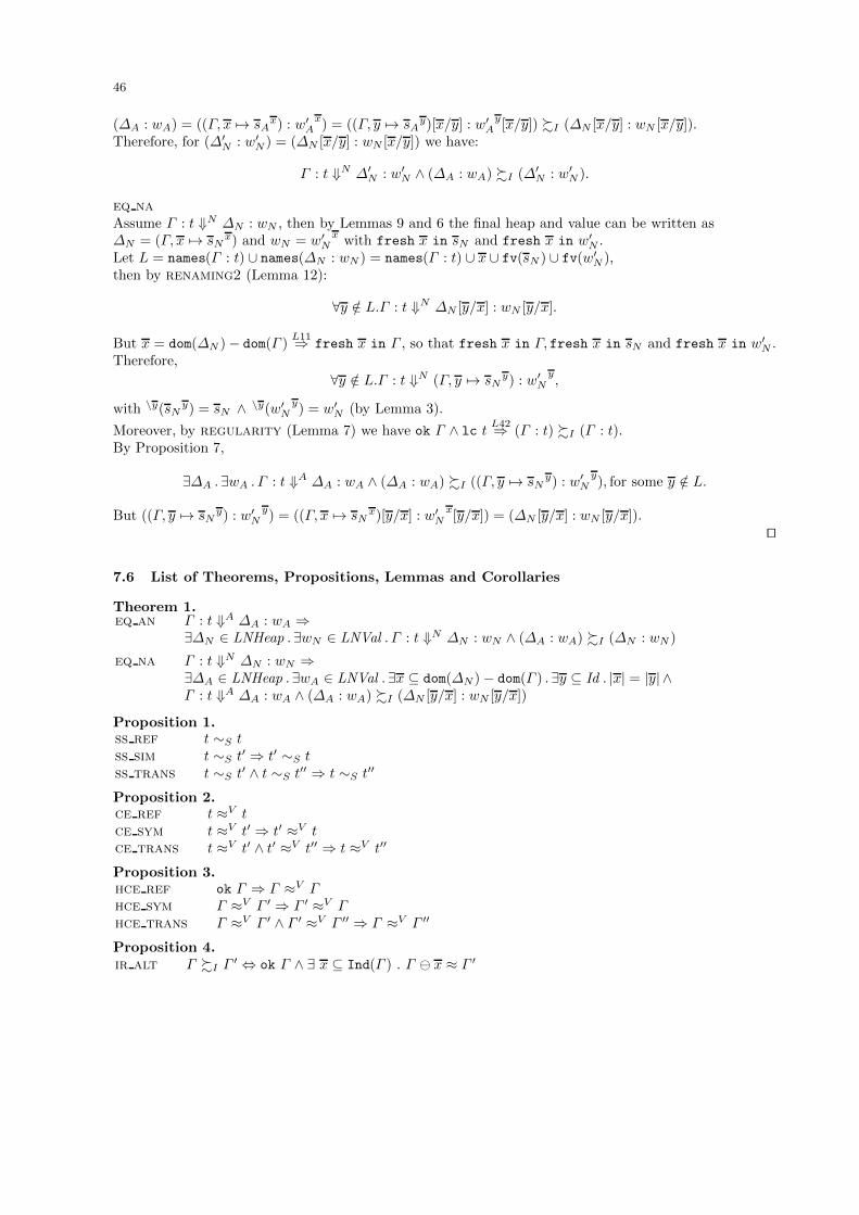
46
(∆A : wA) = ((Γ, x 7→ sAx) : w′
Ax) = ((Γ, y 7→ sA
y)[x/y] : w′Ay[x/y]) %I (∆N [x/y] : wN [x/y]).
Therefore, for (∆′N : w′
N ) = (∆N [x/y] : wN [x/y]) we have:
Γ : t ⇓N ∆′N : w′
N ∧ (∆A : wA) %I (∆′N : w′
N ).
eq naAssume Γ : t ⇓N ∆N : wN , then by Lemmas 9 and 6 the final heap and value can be written as∆N = (Γ, x 7→ sN
x) and wN = w′N
xwith fresh x in sN and fresh x in w′
N .Let L = names(Γ : t) ∪ names(∆N : wN ) = names(Γ : t) ∪ x ∪ fv(sN ) ∪ fv(w′
N ),then by renaming2 (Lemma 12):
∀y /∈ L.Γ : t ⇓N ∆N [y/x] : wN [y/x].
But x = dom(∆N )− dom(Γ )L11⇒ fresh x in Γ , so that fresh x in Γ, fresh x in sN and fresh x in w′
N .Therefore,
∀y /∈ L.Γ : t ⇓N (Γ, y 7→ sNy) : w′
Ny,
with \y(sNy) = sN ∧ \y(w′N
y) = w′
N (by Lemma 3).
Moreover, by regularity (Lemma 7) we have ok Γ ∧ lc tL42⇒ (Γ : t) %I (Γ : t).
By Proposition 7,
∃∆A . ∃wA . Γ : t ⇓A ∆A : wA ∧ (∆A : wA) %I ((Γ, y 7→ sNy) : w′
Ny), for some y /∈ L.
But ((Γ, y 7→ sNy) : w′
Ny) = ((Γ, x 7→ sN
x)[y/x] : w′N
x[y/x]) = (∆N [y/x] : wN [y/x]).
⊓⊔
7.6 List of Theorems, Propositions, Lemmas and Corollaries
Theorem 1.eq an Γ : t ⇓A ∆A : wA ⇒
∃∆N ∈ LNHeap . ∃wN ∈ LNVal . Γ : t ⇓N ∆N : wN ∧ (∆A : wA) %I (∆N : wN )
eq na Γ : t ⇓N ∆N : wN ⇒∃∆A ∈ LNHeap . ∃wA ∈ LNVal . ∃x ⊆ dom(∆N )− dom(Γ ) . ∃y ⊆ Id . |x| = |y| ∧Γ : t ⇓A ∆A : wA ∧ (∆A : wA) %I (∆N [y/x] : wN [y/x])
Proposition 1.ss ref t ∼S tss sim t ∼S t′ ⇒ t′ ∼S tss trans t ∼S t′ ∧ t ∼S t′′ ⇒ t ∼S t′′
Proposition 2.ce ref t ≈V tce sym t ≈V t′ ⇒ t′ ≈V tce trans t ≈V t′ ∧ t′ ≈V t′′ ⇒ t ≈V t′′
Proposition 3.hce ref ok Γ ⇒ Γ ≈V Γhce sym Γ ≈V Γ ′ ⇒ Γ ′ ≈V Γhce trans Γ ≈V Γ ′ ∧ Γ ′ ≈V Γ ′′ ⇒ Γ ≈V Γ ′′
Proposition 4.ir alt Γ %I Γ ′ ⇔ ok Γ ∧ ∃ x ⊆ Ind(Γ ) . Γ ⊖ x ≈ Γ ′
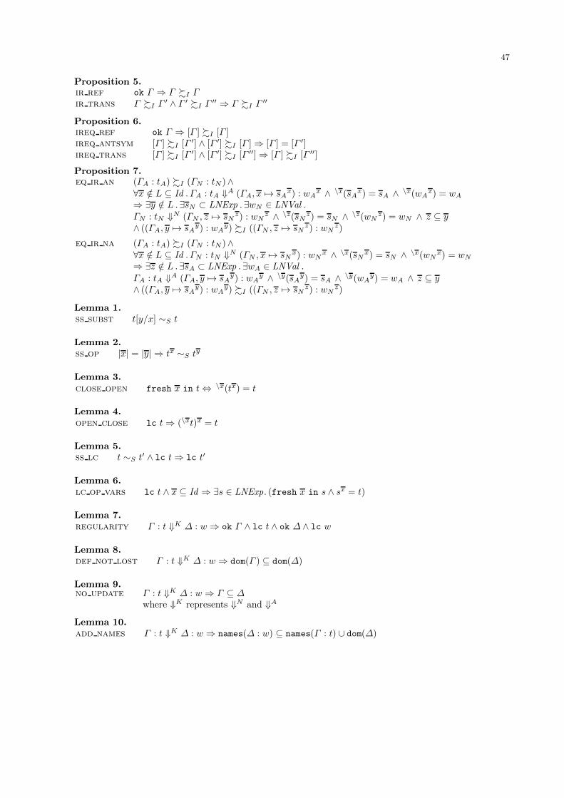
47
Proposition 5.ir ref ok Γ ⇒ Γ %I Γir trans Γ %I Γ ′ ∧ Γ ′ %I Γ ′′ ⇒ Γ %I Γ ′′
Proposition 6.ireq ref ok Γ ⇒ [Γ ] %I [Γ ]ireq antsym [Γ ] %I [Γ ′] ∧ [Γ ′] %I [Γ ]⇒ [Γ ] = [Γ ′]ireq trans [Γ ] %I [Γ ′] ∧ [Γ ′] %I [Γ ′′]⇒ [Γ ] %I [Γ ′′]
Proposition 7.eq ir an (ΓA : tA) %I (ΓN : tN )∧
∀x /∈ L ⊆ Id . ΓA : tA ⇓A (ΓA, x 7→ sAx) : wA
x ∧ \x(sAx) = sA ∧ \x(wA
x) = wA
⇒ ∃y /∈ L . ∃sN ⊂ LNExp . ∃wN ∈ LNVal .
ΓN : tN ⇓N (ΓN , z 7→ sNz) : wN
z ∧ \z(sNz) = sN ∧ \z(wNz) = wN ∧ z ⊆ y
∧ ((ΓA, y 7→ sAy) : wA
y) %I ((ΓN , z 7→ sNz) : wN
z)
eq ir na (ΓA : tA) %I (ΓN : tN )∧∀x /∈ L ⊆ Id . ΓN : tN ⇓N (ΓN , x 7→ sN
x) : wNx ∧ \x(sN
x) = sN ∧ \x(wNx) = wN
⇒ ∃z /∈ L . ∃sA ⊂ LNExp . ∃wA ∈ LNVal .
ΓA : tA ⇓A (ΓA, y 7→ sAy) : wA
y ∧ \y(sAy) = sA ∧ \y(wAy) = wA ∧ z ⊆ y
∧ ((ΓA, y 7→ sAy) : wA
y) %I ((ΓN , z 7→ sNz) : wN
z)
Lemma 1.ss subst t[y/x] ∼S t
Lemma 2.ss op |x| = |y| ⇒ tx ∼S ty
Lemma 3.close open fresh x in t⇔ \x(tx) = t
Lemma 4.open close lc t⇒ (\xt)x = t
Lemma 5.ss lc t ∼S t′ ∧ lc t⇒ lc t′
Lemma 6.lc op vars lc t ∧ x ⊆ Id ⇒ ∃s ∈ LNExp. (fresh x in s ∧ sx = t)
Lemma 7.regularity Γ : t ⇓K ∆ : w ⇒ ok Γ ∧ lc t ∧ ok ∆ ∧ lc w
Lemma 8.def not lost Γ : t ⇓K ∆ : w ⇒ dom(Γ ) ⊆ dom(∆)
Lemma 9.no update Γ : t ⇓K ∆ : w ⇒ Γ ⊆ ∆
where ⇓K represents ⇓N and ⇓A
Lemma 10.add names Γ : t ⇓K ∆ : w ⇒ names(∆ : w) ⊆ names(Γ : t) ∪ dom(∆)

48
Lemma 11.new names1 Γ : t ⇓N ∆ : w ∧ x ∈ dom(∆)− dom(Γ )⇒ fresh x in Γnew names2 Γ : t ⇓A ∆ : w ∧ x ∈ dom(∆)− dom(Γ )⇒ fresh x in (Γ : t)
Lemma 12.renaming1 Γ : t ⇓K ∆ : w ∧ fresh y in (Γ : t) ∧ fresh y in (∆ : w)
⇒ Γ [y/x] : t[y/x] ⇓K ∆[y/x] : w[y/x]
renaming2 Γ : t ⇓K ∆ : w ∧ fresh y in (Γ : t) ∧ fresh y in (∆ : w) ∧ x /∈ dom(Γ ) ∧ x ∈ dom(∆)⇒ Γ : t ⇓K ∆[y/x] : w[y/x]
Lemma 13.ce ss t ≈V t′ ⇒ t ∼S t′
Lemma 14.ce sub t ≈V t′ ∧ V ′ ⊆ V ⇒ t ≈V ′
t′
ce add t ≈V t′ ∧ fresh x in t ∧ fresh x in t′ ⇒ t ≈V ∪x t′
Lemma 15.ce subs1 t ≈V t′ ∧ x, y /∈ V ⇒ t[y/x] ≈V t′
ce subs2 t ≈V t′ ∧ (fvar y) ≈V (fvar y′) ∧ x ∈ V ⇒ t[y/x] ≈V t′[y′/x]
ce subs3 t ≈V t′ ∧ y /∈ V ∧ fresh y in t ∧ fresh y in t′ ⇒ t[y/x] ≈V [y/x] t′[y/x]
ce op1 t ≈V t′ ⇒ tx ≈V t′x
ce op2 t ≈V t′ ∧ x, y /∈ V ∧ |x| = |y| ⇒ tx ≈V t′y
ce op3 t ≈V t′ ∧ (fvar x) ≈V (fvar y)⇒ tx ≈V t′y
Lemma 16.hce dom Γ ≈V Γ ′ ⇒ dom(Γ ) = dom(Γ ′)hce ind Γ ≈V Γ ′ ⇒ Ind(Γ ) = Ind(Γ ′)hce ok Γ ≈V Γ ′ ⇒ ok Γ ∧ ok Γ ′
Lemma 17.hce alt Γ ≈V Γ ′ ⇔ ok Γ ∧ ok Γ ′ ∧ dom(Γ ) = dom(Γ ′) ∧ (x 7→ t ∈ Γ ∧ x 7→ t′ ∈ Γ ′ ⇒ t ≈V t′)
Lemma 18.hce swap ok Γ ∧ x, y ∈ Ind(Γ ) ∧ x 6= y ⇒ Γ ⊖ [x, y] ≈V −{x,y} Γ ⊖ [y, x]
Lemma 19.he perm ok Γ ∧ x, y ∈ Ind(Γ )⇒ (Γ ⊖ x ≈ Γ ⊖ y ⇔ y ∈ S(x))
Lemma 20.ir dom Γ %I Γ ′ ⇒ dom(Γ ′) ⊆ dom(Γ )ir ind Γ %I Γ ′ ⇒ Ind(Γ ′) ⊆ Ind(Γ )ir ok Γ %I Γ ′ ⇒ ok Γ ∧ ok Γ ′
ir dom he Γ %I Γ ′ ∧ dom(Γ ) = dom(Γ ′)⇒ Γ ≈ Γ ′
ir ir he (Γ %I Γ ′ ∧ Γ ′ %I Γ )⇔ Γ ≈ Γ ′
Lemma 21.ireq he ireq1 [Γ ] %I [Γ ′] ∧∆ ≈ Γ ⇒ [∆] %I [Γ ′]ireq he ireq2 [Γ ] %I [Γ ′] ∧∆ ≈ Γ ′ ⇒ [Γ ] %I [∆]
Lemma 22.irht irh (Γ : t) %I (Γ ′ : t′)⇒ Γ %I Γ ′
irht ss (Γ : t) %I (Γ ′ : t′)⇒ t ∼S t′
irht lc (Γ : t) %I (Γ ′ : t′)⇒ lc t ∧ lc t′

49
Lemma 23.ss opk t ∼S t′ ∧ |x| = |y| ⇒ {k→ x}t ∼S {k→ y}t′
Lemma 24.opk clk fresh {k ← x}({k→ x}t) = t⇒ fresh x in t
Lemma 25.lc opk vars lc at k n t ∧ x ⊆ Id ⇒ ∃s ∈ LNExp. (fresh x in s ∧ {k→ x}s = t)
Lemma 26.keep names Γ : t ⇓A ∆ : w ⇒ fv(t) ⊆ names(∆ : w)
Lemma 27.ce opk1 t ≈V t′ ⇒ {k → x}t ≈V {k → x}t′ce opk2 t ≈V t′ ∧ x, y /∈ V ∧ |x| = |y| ⇒ {k → x}t ≈V {k→ y}t′
Lemma 28.hce bind (Γ, x 7→ t) ≈V (Γ ′, x 7→ t′)⇒ Γ ≈V Γ ′ ∧ t ≈V t′
Lemma 29.ind dom ok Γ ∧ x ∈ Ind(Γ )⇒ dom(Γ ⊖ x) = dom(Γ )− {x} ∧ Ind(Γ ⊖ x) = Ind(Γ )− {x}
Lemma 30.ind ok ok Γ ∧ x ∈ Ind(Γ )⇒ ok (Γ ⊖ x)
Lemma 31.ind subs x /∈ dom(Γ )⇒ (Γ, x 7→ fvar y)⊖ x = Γ [y/x]
Lemma 32.hce sub Γ ≈V Γ ′ ∧ V ′ ⊆ V ⇒ Γ ≈V ′
Γ ′
hce add Γ ≈V Γ ′ ∧ x /∈ names(Γ ) ∪ names(Γ ′)⇒ Γ ≈V ∪x Γ ′
Lemma 33.hce del ind Γ ≈V Γ ′ ∧ dom(Γ ) ⊆ V ∧ x ∈ Ind(Γ )⇒ Γ ⊖ x ≈V Γ ′ ⊖ xhe del ind Γ ≈ Γ ′ ∧ x ∈ Ind(Γ )⇒ Γ ⊖ x ≈ Γ ′ ⊖ x
Lemma 34.ir fvar (Γ : fvar x) %I (Γ ′ : fvar x′)
⇒ (x /∈ dom(Γ ) ∧ x′ /∈ dom(Γ ′))∨ (x ∈ dom(Γ ) ∧ x′ ∈ dom(Γ ′)∧∃x0, . . . , xn ∈ Id . x0 = x ∧ xn = x′ ∧ ∀i : 0 ≤ i < n . xi 7→ fvar xi+1 ∈ Γ )
Lemma 35.ir irht (Γ, x 7→ t) %I (Γ ′, x 7→ t′)⇒ ((Γ, x 7→ t) : t) %I ((Γ ′, x 7→ t′) : t′).
Lemma 36.ir fvar irht ((Γ, x 7→ t) : fvar x) %I ((Γ ′, x′ 7→ t′) : fvar x′)
⇒ ((Γ, x 7→ t) : t) %I ((Γ ′, x′ 7→ t′) : t′) ∨ ((Γ, x 7→ t) : t) %I ((Γ ′, x′ 7→ t′) : fvar x′).
Lemma 37.irht app (Γ : app t (fvar x)) %I (Γ ′ : app t′ (fvar x′))
⇒ (Γ : t) %I (Γ ′ : t′) ∧ (Γ : fvar x) %I (Γ ′ : fvar x′).

50
Lemma 38.irht fv (Γ : fvar x) %I (Γ ′ : fvar x′) ∧ Γ ⊆ ∆ ∧ Γ ′ ⊆ ∆′ ∧∆ %I ∆′∧
(x /∈ dom(Γ )⇒ x /∈ dom(∆)) ∧ (x′ /∈ dom(Γ ′)⇒ x′ /∈ dom(∆′))∧(y ∈ dom(Γ ) ∧ y /∈ dom(Γ ′)⇒ y /∈ dom(∆′))⇒ (∆ : fvar x) %I (∆′ : fvar x′).
Lemma 39.irht red ind fresh y in (Γ : t) ∧ y 6= x ∧ (Γ : abs t) %I (Γ ′ : abs t′) ∧ (Γ : fvar x) %I (Γ ′ : fvar x′)
⇒ ((Γ, y 7→ fvar x) : ty) %I (Γ ′ : t′x′).
Lemma 40.intr vars fresh x in (Γ : let t in t) ∧ fresh x in (Γ ′ : let t′ in t′)∧
(Γ : let t in t) %I (Γ ′ : let t′ in t′)⇒ ((Γ, x 7→ tx) : tx) %I ((Γ ′, x 7→ t′
x) : t′x).
Lemma 41.hce subs Γ ≈V Γ ′ ∧ y /∈ V ∧ fresh y in Γ ∧ fresh y in Γ ′ ⇒ Γ [y/x] ≈V [y/x] Γ ′[y/x]ir subs Γ %I Γ ′ ∧ fresh y in Γ ∧ fresh y in Γ ′ ⇒ Γ [y/x] %I Γ ′[y/x]ir ht subs (Γ : t) %I (Γ ′ : t′) ∧ fresh y in (Γ : t) ∧ fresh y in (Γ ′ : t′)
⇒ (Γ [y/x] : t[y/x]) %I (Γ ′[y/x] : t′[y/x])
Lemma 42.irht ref ok Γ ∧ lc t⇒ (Γ : t) %I (Γ : t)
Corollary 1.ir dom dom Γ %I Γ ′ ⇒ Γ ⊖ (dom(Γ )− dom(Γ ′)) ≈ Γ ′
Corollary 2.renaming3 Γ : t ⇓K ∆ : w ∧ fresh y in (Γ : t) ∧ fresh y in (∆ : w) ∧ x /∈ names(Γ : t)
⇒ Γ : t ⇓K ∆[y/x] : w[y/x]
Corollary 3.ce lc t ≈V t′ ∧ lc t⇒ lc t′
Apendice B
Trabajo en progreso
En este segundo apendice se incluyen dos trabajos en progreso (WP1 [SGHHOM14a] yWP2 [SGHHOM12a]) que fueron presentados en sendas ediciones de las Jornadas de Pro-gramacion y Lenguajes (PROLE) y publicados en las correspondientes actas. El primerode ellos, Launchbury’s semantics revisited: On the equivalence of context-heap semantics,ha sido presentado en Cadiz en septiembre de 2014. En el se recopilan las principales ideasde las publicaciones P2 y P3 y se introduce el estudio que se esta realizando actualmentesobre el efecto de actualizar o no las clausuras durante la evaluacion. Se concluye conA formalization in Coq of Launchbury’s natural semantics for lazy evaluation, presenta-do en Almerıa en septiembre de 2012. Este trabajo muestra los primeros pasos hacia laimplementacion en Coq de los resultados obtenidos en los trabajos sobre las semanticas.
Two works in progress, (WP1 [SGHHOM14a] and WP2 [SGHHOM12a]), appear in thissecond appendix. They were presented in Jornadas de Programacion y Lenguajes (PROLE)in 2014 and 2012, respectively. Both were published in the corresponding proceedings ofthe workshops. The first work, Launchbury’s semantics revisited: On the equivalence ofcontext-heap semantics was presented in Cadiz in September 2014, and collects the mainideas of publications P2 and P3. This paper also contains some of the results that we havealready obtained on the effects of updating closures during evaluation. We conclude withA formalization in Coq of Launchbury’s natural semantics for lazy evaluation presentedin Almeria in September 2012. This work shows the first steps on the implementation inthe proof assistant Coq of some of our results on semantics for lazy evaluation.
249

250 Capıtulo B. Trabajo en progreso

Submitted to:PROLE 2014
c© L. Sanchez-Gil, M. Hidalgo-Herrero & Y. Ortega-MallenThis work is licensed under theCreative Commons Attribution License.
Launchbury’s semantics revisited: On the equivalence ofcontext-heap semantics
(Work in progress)
Lidia Sanchez-GilFacultad de Informatica
Universidad Complutense de MadridEspana
Mercedes Hidalgo-HerreroFacultad de Educacion
Universidad Complutense de MadridEspana
Yolanda Ortega-MallenFacultad de CC. Matematicas
Universidad Complutense de MadridEspana
Launchbury’s natural semantics for lazy evaluation is based on heaps of bindings, i.e., variable-expression pairs, which define the evaluation context. In order to prove the adequacy of the opera-tional semantics with respect to a standard denotational one, Lauchbury defines an alternative naturalsemantics where updating of bindings is removed andβ -reduction is done through indirections in-stead of variable substitution. We study how context heaps are affected by these changes, and wedefine several relations between heaps. These relations allow to establish the equivalence betweenLaunchbury’s natural semantics and its alternative version. This result is crucial because many au-thors have based their proofs on its veracity.
1 Motivation
More than twenty years have elapsed since Launchbury first presented in [9] his natural semantics forlazy evaluation, a key contribution to the semantic foundation for non-strict functional programminglanguages like Haskell or Clean. Throughout these years, Launchbury’s natural semantics has been citedfrequently and has inspired many further works as well as several extensions like in [2, 10, 18, 8]. Theauthors have extended in [13] Launchbury’s semantics with rules forparallel applicationthat creates newprocesses to distribute the computation; these distributed processes exchange values through communi-cation channels. The success of Lanchbury’s proposal resides in its simplicity. Expressions are evaluatedwith respect to acontext, which is represented by a heap ofbindings, that is, (variable, expression) pairs.This heap is explicitly managed to make possible the sharingof bindings, thus, modeling laziness.
In order to prove that this lazy (operational) semantics iscorrectandcomputationally adequatewithrespect to a standard denotational semantics, Launchbury introduces some variations in the operationalsemantics. On the one hand, the update of bindings with theircomputed values is an operational notionwithout counterpart in the standard denotational semantics, so that the alternative natural semantics doesno longer update bindings and becomes acall-by-namesemantics. On the other hand, functional appli-cation is modeled denotationally by extending the environment with a variable bound to a value. Thisnew variable represents the formal parameter of the function, while the value corresponds to the actualargument. For a closer approach to this mechanism, in the alternative operational semantics applications
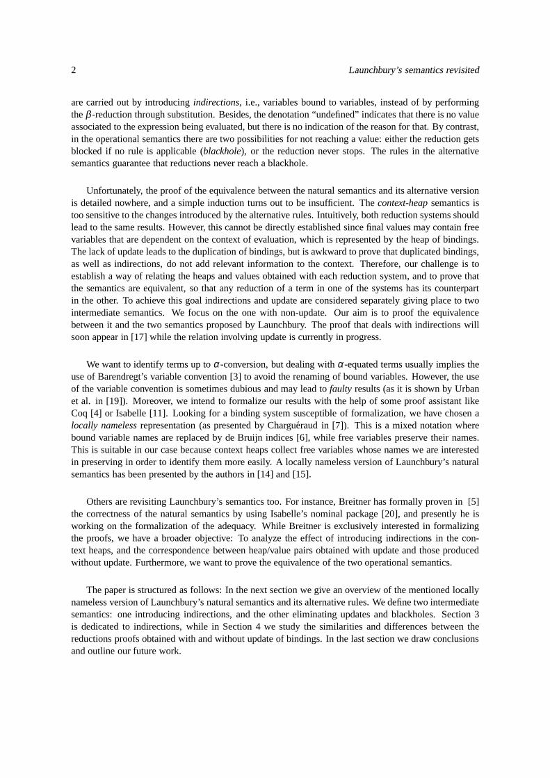
2 Launchbury’s semantics revisited
are carried out by introducingindirections, i.e., variables bound to variables, instead of by performingtheβ -reduction through substitution. Besides, the denotation“undefined” indicates that there is no valueassociated to the expression being evaluated, but there is no indication of the reason for that. By contrast,in the operational semantics there are two possibilities for not reaching a value: either the reduction getsblocked if no rule is applicable (blackhole), or the reduction never stops. The rules in the alternativesemantics guarantee that reductions never reach a blackhole.
Unfortunately, the proof of the equivalence between the natural semantics and its alternative versionis detailed nowhere, and a simple induction turns out to be insufficient. Thecontext-heapsemantics istoo sensitive to the changes introduced by the alternative rules. Intuitively, both reduction systems shouldlead to the same results. However, this cannot be directly established since final values may contain freevariables that are dependent on the context of evaluation, which is represented by the heap of bindings.The lack of update leads to the duplication of bindings, but is awkward to prove that duplicated bindings,as well as indirections, do not add relevant information to the context. Therefore, our challenge is toestablish a way of relating the heaps and values obtained with each reduction system, and to prove thatthe semantics are equivalent, so that any reduction of a termin one of the systems has its counterpartin the other. To achieve this goal indirections and update are considered separately giving place to twointermediate semantics. We focus on the one with non-update. Our aim is to proof the equivalencebetween it and the two semantics proposed by Launchbury. Theproof that deals with indirections willsoon appear in [17] while the relation involving update is currently in progress.
We want to identify terms up toα-conversion, but dealing withα-equated terms usually implies theuse of Barendregt’s variable convention [3] to avoid the renaming of bound variables. However, the useof the variable convention is sometimes dubious and may leadto faulty results (as it is shown by Urbanet al. in [19]). Moreover, we intend to formalize our resultswith the help of some proof assistant likeCoq [4] or Isabelle [11]. Looking for a binding system susceptible of formalization, we have chosen alocally namelessrepresentation (as presented by Chargueraud in [7]). Thisis a mixed notation wherebound variable names are replaced by de Bruijn indices [6], while free variables preserve their names.This is suitable in our case because context heaps collect free variables whose names we are interestedin preserving in order to identify them more easily. A locally nameless version of Launchbury’s naturalsemantics has been presented by the authors in [14] and [15].
Others are revisiting Launchbury’s semantics too. For instance, Breitner has formally proven in [5]the correctness of the natural semantics by using Isabelle’s nominal package [20], and presently he isworking on the formalization of the adequacy. While Breitner is exclusively interested in formalizingthe proofs, we have a broader objective: To analyze the effect of introducing indirections in the con-text heaps, and the correspondence between heap/value pairs obtained with update and those producedwithout update. Furthermore, we want to prove the equivalence of the two operational semantics.
The paper is structured as follows: In the next section we give an overview of the mentioned locallynameless version of Launchbury’s natural semantics and itsalternative rules. We define two intermediatesemantics: one introducing indirections, and the other eliminating updates and blackholes. Section 3is dedicated to indirections, while in Section 4 we study thesimilarities and differences between thereductions proofs obtained with and without update of bindings. In the last section we draw conclusionsand outline our future work.
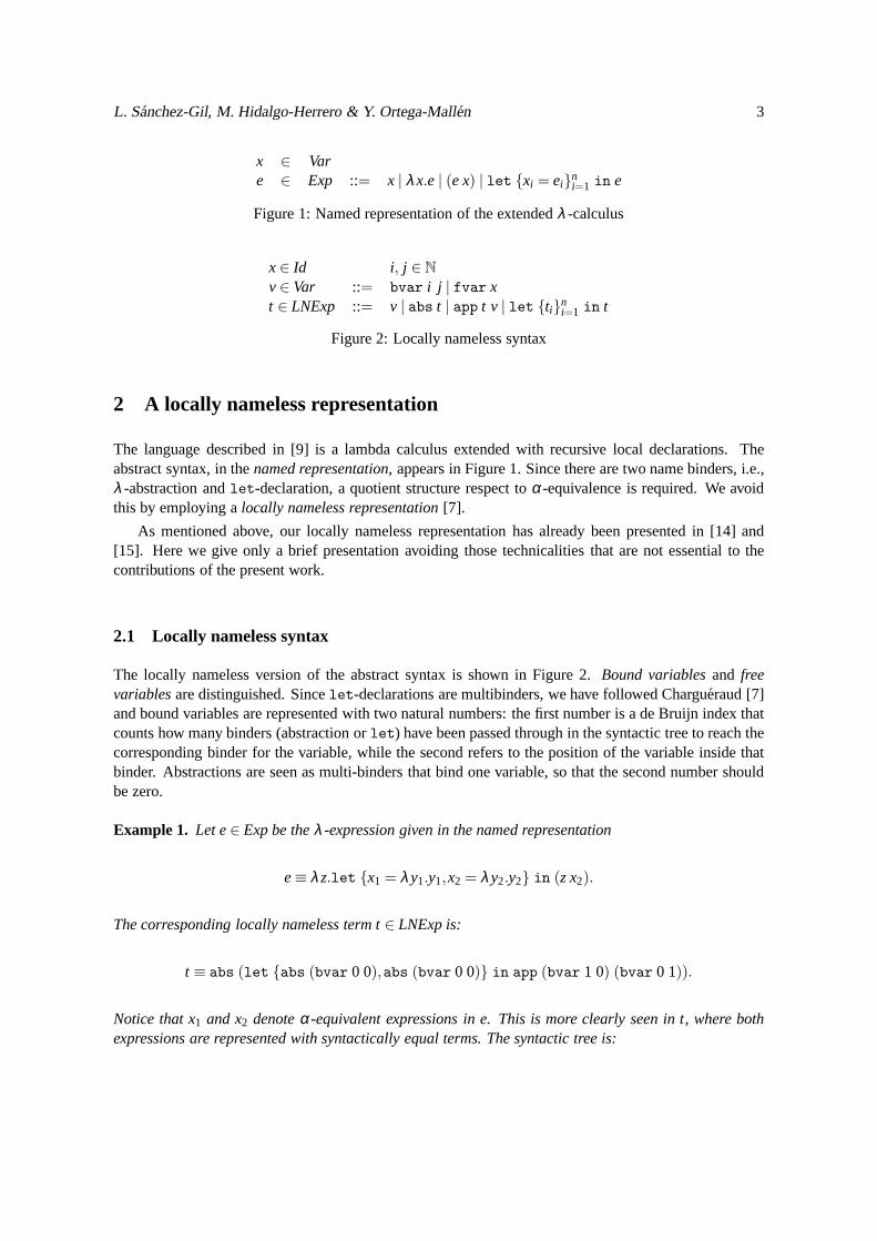
L. Sanchez-Gil, M. Hidalgo-Herrero & Y. Ortega-Mallen 3
x ∈ Vare ∈ Exp ::= x | λx.e | (e x) | let {xi = ei}n
i=1 in e
Figure 1: Named representation of the extendedλ -calculus
x∈ Id i, j ∈ Nv∈ Var ::= bvar i j | fvar xt ∈ LNExp ::= v | abs t | app t v | let {ti}n
i=1 in t
Figure 2: Locally nameless syntax
2 A locally nameless representation
The language described in [9] is a lambda calculus extended with recursive local declarations. Theabstract syntax, in thenamed representation, appears in Figure 1. Since there are two name binders, i.e.,λ -abstraction andlet-declaration, a quotient structure respect toα-equivalence is required. We avoidthis by employing alocally nameless representation[7].
As mentioned above, our locally nameless representation has already been presented in [14] and[15]. Here we give only a brief presentation avoiding those technicalities that are not essential to thecontributions of the present work.
2.1 Locally nameless syntax
The locally nameless version of the abstract syntax is shownin Figure 2. Bound variablesand freevariablesare distinguished. Sincelet-declarations are multibinders, we have followed Chargueraud [7]and bound variables are represented with two natural numbers: the first number is a de Bruijn index thatcounts how many binders (abstraction orlet) have been passed through in the syntactic tree to reach thecorresponding binder for the variable, while the second refers to the position of the variable inside thatbinder. Abstractions are seen as multi-binders that bind one variable, so that the second number shouldbe zero.
Example 1. Let e∈ Exp be theλ -expression given in the named representation
e≡ λz.let {x1 = λy1.y1,x2 = λy2.y2} in (z x2).
The corresponding locally nameless term t∈ LNExp is:
t ≡ abs (let {abs (bvar 0 0),abs (bvar 0 0)} in app (bvar 1 0) (bvar 0 1)).
Notice that x1 and x2 denoteα-equivalent expressions in e. This is more clearly seen in t,where bothexpressions are represented with syntactically equal terms. The syntactic tree is:
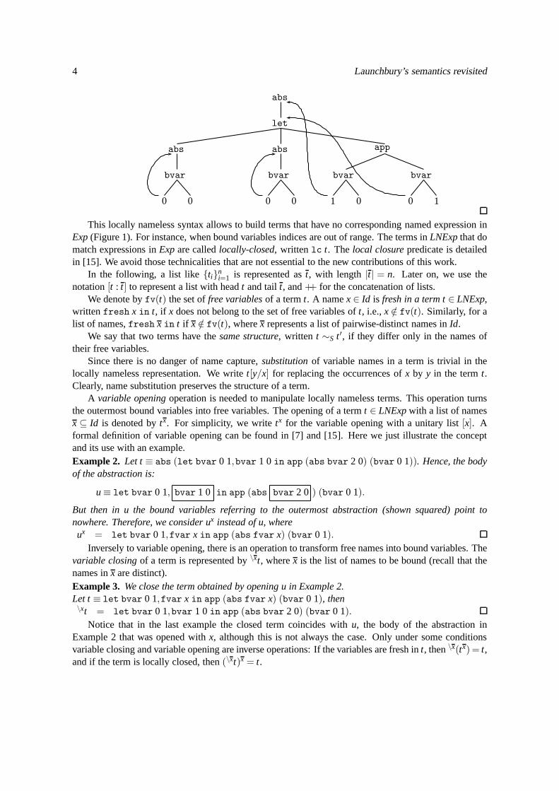
4 Launchbury’s semantics revisited
abs
let
abs abs app
bvar bvar bvar bvar
0 0 0 0 01 0 1
This locally nameless syntax allows to build terms that haveno corresponding named expression inExp(Figure 1). For instance, when bound variables indices are out of range. The terms inLNExpthat domatch expressions inExpare calledlocally-closed, writtenlc t. The local closurepredicate is detailedin [15]. We avoid those technicalities that are not essential to the new contributions of this work.
In the following, a list like{ti}ni=1 is represented ast, with length |t| = n. Later on, we use the
notation[t : t] to represent a list with headt and tailt, and++ for the concatenation of lists.We denote byfv(t) the set offree variablesof a termt. A namex∈ Id is fresh in a term t∈ LNExp,
written fresh x in t, if x does not belong to the set of free variables oft, i.e.,x /∈ fv(t). Similarly, for alist of names,fresh x in t if x /∈ fv(t), wherex represents a list of pairwise-distinct names inId.
We say that two terms have thesame structure, written t ∼S t ′, if they differ only in the names oftheir free variables.
Since there is no danger of name capture,substitutionof variable names in a term is trivial in thelocally nameless representation. We writet[y/x] for replacing the occurrences ofx by y in the termt.Clearly, name substitution preserves the structure of a term.
A variable openingoperation is needed to manipulate locally nameless terms. This operation turnsthe outermost bound variables into free variables. The opening of a termt ∈ LNExpwith a list of namesx ⊆ Id is denoted bytx. For simplicity, we writetx for the variable opening with a unitary list[x]. Aformal definition of variable opening can be found in [7] and [15]. Here we just illustrate the conceptand its use with an example.Example 2. Let t≡ abs (let bvar 0 1,bvar 1 0in app (abs bvar 2 0) (bvar 0 1)). Hence, the bodyof the abstraction is:
u≡ let bvar 0 1, bvar 1 0 in app (abs bvar 2 0 ) (bvar 0 1).
But then in u the bound variables referring to the outermost abstraction (shown squared) point tonowhere. Therefore, we consider ux instead of u, whereux = let bvar 0 1,fvar x in app (abs fvar x) (bvar 0 1).
Inversely to variable opening, there is an operation to transform free names into bound variables. Thevariable closingof a term is represented by\xt, wherex is the list of names to be bound (recall that thenames inx are distinct).Example 3. We close the term obtained by opening u in Example 2.Let t≡ let bvar 0 1,fvar x in app (abs fvar x) (bvar 0 1), then\xt = let bvar 0 1,bvar 1 0in app (abs bvar 2 0) (bvar 0 1).
Notice that in the last example the closed term coincides with u, the body of the abstraction inExample 2 that was opened withx, although this is not always the case. Only under some conditionsvariable closing and variable opening are inverse operations: If the variables are fresh int, then\x(tx) = t,and if the term is locally closed, then(\xt)x = t.
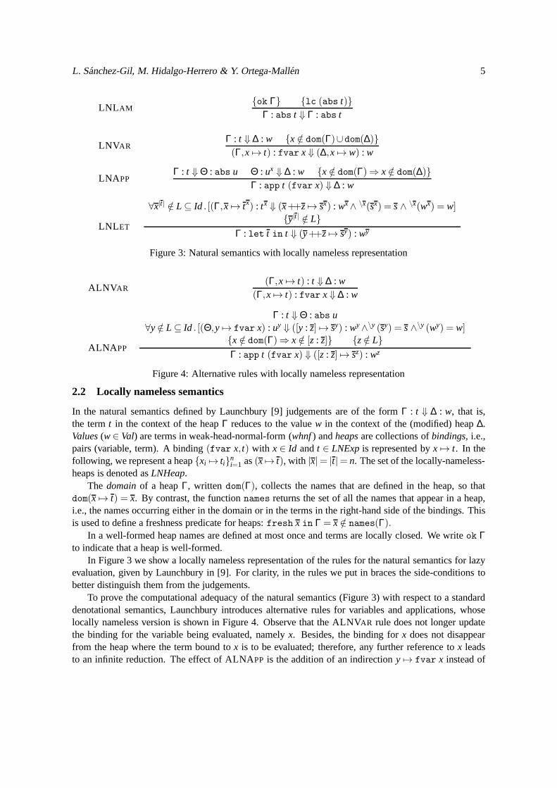
L. Sanchez-Gil, M. Hidalgo-Herrero & Y. Ortega-Mallen 5
LNL AM{ok Γ} {lc (abs t)}
Γ : abs t ⇓ Γ : abs t
LNVARΓ : t ⇓ ∆ : w {x /∈ dom(Γ)∪dom(∆)}(Γ,x 7→ t) : fvar x⇓ (∆,x 7→ w) : w
LNA PPΓ : t ⇓ Θ : abs u Θ : ux ⇓ ∆ : w {x /∈ dom(Γ) ⇒ x /∈ dom(∆)}
Γ : app t (fvar x) ⇓ ∆ : w
LNL ET
∀x|t | /∈ L ⊆ Id . [(Γ,x 7→ tx) : tx ⇓ (x++z 7→ sx) : wx∧ \x(sx) = s∧ \x(wx) = w]
{y|t | /∈ L}Γ : let t in t ⇓ (y++z 7→ sy) : wy
Figure 3: Natural semantics with locally nameless representation
ALNVAR(Γ,x 7→ t) : t ⇓ ∆ : w
(Γ,x 7→ t) : fvar x⇓ ∆ : w
ALNA PP
Γ : t ⇓ Θ : abs u∀y /∈ L ⊆ Id . [(Θ,y 7→ fvar x) : uy ⇓ ([y : z] 7→ sy) : wy∧\y (sy) = s∧\y (wy) = w]
{x /∈ dom(Γ) ⇒ x /∈ [z : z]} {z /∈ L}Γ : app t (fvar x) ⇓ ([z : z] 7→ sz) : wz
Figure 4: Alternative rules with locally nameless representation
2.2 Locally nameless semantics
In the natural semantics defined by Launchbury [9] judgements are of the formΓ : t ⇓ ∆ : w, that is,the termt in the context of the heapΓ reduces to the valuew in the context of the (modified) heap∆.Values(w∈ Val) are terms in weak-head-normal-form (whnf) andheapsare collections ofbindings, i.e.,pairs (variable, term). A binding(fvar x, t) with x∈ Id andt ∈ LNExpis represented byx 7→ t. In thefollowing, we represent a heap{xi 7→ ti}n
i=1 as(x 7→ t), with |x|= |t|= n. The set of the locally-nameless-heaps is denoted asLNHeap.
The domainof a heapΓ, written dom(Γ), collects the names that are defined in the heap, so thatdom(x 7→ t) = x. By contrast, the functionnames returns the set of all the names that appear in a heap,i.e., the names occurring either in the domain or in the termsin the right-hand side of the bindings. Thisis used to define a freshness predicate for heaps:fresh x in Γ = x /∈ names(Γ).
In a well-formed heap names are defined at most once and terms are locally closed. We writeok Γto indicate that a heap is well-formed.
In Figure 3 we show a locally nameless representation of the rules for the natural semantics for lazyevaluation, given by Launchbury in [9]. For clarity, in the rules we put in braces the side-conditions tobetter distinguish them from the judgements.
To prove the computational adequacy of the natural semantics (Figure 3) with respect to a standarddenotational semantics, Launchbury introduces alternative rules for variables and applications, whoselocally nameless version is shown in Figure 4. Observe that the ALNVAR rule does not longer updatethe binding for the variable being evaluated, namelyx. Besides, the binding forx does not disappearfrom the heap where the term bound tox is to be evaluated; therefore, any further reference tox leadsto an infinite reduction. The effect of ALNAPP is the addition of an indirectiony 7→ fvar x instead of

6 Launchbury’s semantics revisited
NS INS NNS ANS
Indirections # ! # !Update ! ! # #Blackholes ! ! # #
Figure 5: The lazy natural semantics and its alternatives
performing theβ -reduction by substitution, as inux in LNA PP.In the rules LNLET and ALNAPP we usecofinite quantification[1], which is an alternative to
“exists-fresh” quantifications that provides stronger induction and inversion principles. Although thereare not explicit freshness side-conditions in the rules, the finite setL represents somehow the names thatshould be avoided during a reduction proof. We use the variable opening to express that the final heapand value may depend on the chosen names. For instance, in LNLET, wx indicates that the final valuedepends on the namesx, but there is a common basisw. Moreover, it is required that this basis does notcontain occurrences ofx; this is is expressed by\x(wx) = w. A detailed explanation of these semanticrules can be found in [14, 15].
In the following, the natural semantics (rules in Figure 3) is referred as NS, and the alternativesemantics (rules LNLAM , LNL ET and those in Figure 4) as ANS. We write⇓A for reductions in ANS.Launchbury proves in [9] the correctness of NS with respect to a standard denotational semantics, anda similar result for ANS is easily obtained (as the authors ofthis paper have done in [12]). Therefore,NS and ANS are “denotationally” equivalent in the sense thatif an expression is reducible (in some heapcontext) by both semantics then the obtained values have thesame denotation. But this is insufficientfor our purposes, because we want to ensure that if for some (heap : term) pair a reduction exists inany of the semantics, then there must exist a reduction in theother too, and the final heaps must berelated. The changes introduced by ANS might seem to involveno serious difficulties to prove thelatter result. Unfortunately things are not so easy. On the one hand, the alternative rule for variablestransforms the original call-by-need semantics into a call-by-name semantics because bindings are notupdated and computed values are no longer shared. Moreover,in the original semantics the reduction ofa self-reference gets blocked (blackhole), while in the alternative semantics self-references yield infinitereductions. On the other hand, the addition of indirectionscomplicates the task of comparing the (heap :value) pairs obtained by each reduction system, as one may need to follow a chain of indirections to getthe term bound to a variable. We deal separately with each modification and introduce two intermediatesemantics: (1) theNo-update Natural Semantics(NNS) with the rules of NS (Figure 3) except for thevariable rule, that corresponds to the one in the alternative version, i.e., ALNVAR in Figure 4; and (2) theIndirection Natural Semantics(INS) with the rules of NS but for the application rule, that correspondsto the alternative ALNAPP rule in Figure 4. We use⇓N to represent reductions of NNS and⇓I for thoseof INS. Figure 5 resumes the characteristics of the four natural semantics explained above.
It is guaranteed that the judgements produced by the locallynameless rules given in Figures 3 and4 involve only well-formed heaps and locally closed terms. Furthermore, the reduction systems corre-sponding to these rules verify a number of interesting properties proved in [15]. We just show here therenaminglemma, that ensures that the evaluation of a term is independent of the names chosen during thereduction process. Further, any name defined in the context heap can be replaced by a fresh one withoutchanging the meaning of the terms evaluated in that context.In fact, reductions for (heap : term) pairsare unique up toα-conversion of the names defined in the heap.
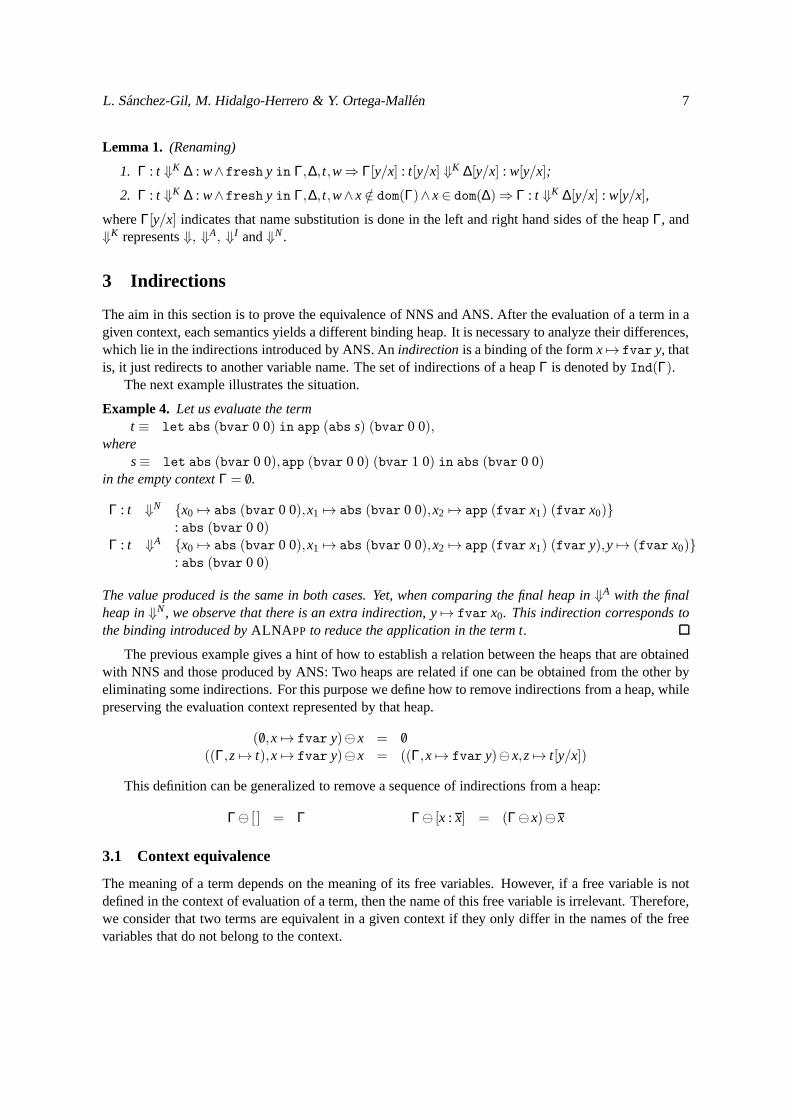
L. Sanchez-Gil, M. Hidalgo-Herrero & Y. Ortega-Mallen 7
Lemma 1. (Renaming)
1. Γ : t ⇓K ∆ : w∧fresh y in Γ,∆, t,w⇒ Γ[y/x] : t[y/x] ⇓K ∆[y/x] : w[y/x];
2. Γ : t ⇓K ∆ : w∧fresh y in Γ,∆, t,w∧x /∈ dom(Γ)∧x∈ dom(∆) ⇒ Γ : t ⇓K ∆[y/x] : w[y/x],
whereΓ[y/x] indicates that name substitution is done in the left and right hand sides of the heapΓ, and⇓K represents⇓, ⇓A, ⇓I and⇓N.
3 Indirections
The aim in this section is to prove the equivalence of NNS and ANS. After the evaluation of a term in agiven context, each semantics yields a different binding heap. It is necessary to analyze their differences,which lie in the indirections introduced by ANS. Anindirection is a binding of the formx 7→ fvar y, thatis, it just redirects to another variable name. The set of indirections of a heapΓ is denoted byInd(Γ).
The next example illustrates the situation.
Example 4. Let us evaluate the termt ≡ let abs (bvar 0 0) in app (abs s) (bvar 0 0),
wheres≡ let abs (bvar 0 0),app (bvar 0 0) (bvar 1 0) in abs (bvar 0 0)
in the empty contextΓ = /0.
Γ : t ⇓N {x0 7→ abs (bvar 0 0),x1 7→ abs (bvar 0 0),x2 7→ app (fvar x1) (fvar x0)}: abs (bvar 0 0)
Γ : t ⇓A {x0 7→ abs (bvar 0 0),x1 7→ abs (bvar 0 0),x2 7→ app (fvar x1) (fvar y),y 7→ (fvar x0)}: abs (bvar 0 0)
The value produced is the same in both cases. Yet, when comparing the final heap in⇓A with the finalheap in⇓N, we observe that there is an extra indirection, y7→ fvar x0. This indirection corresponds tothe binding introduced byALNA PP to reduce the application in the term t.
The previous example gives a hint of how to establish a relation between the heaps that are obtainedwith NNS and those produced by ANS: Two heaps are related if one can be obtained from the other byeliminating some indirections. For this purpose we define how to remove indirections from a heap, whilepreserving the evaluation context represented by that heap.
( /0,x 7→ fvar y)⊖x = /0((Γ,z 7→ t),x 7→ fvar y)⊖x = ((Γ,x 7→ fvar y)⊖x,z 7→ t[y/x])
This definition can be generalized to remove a sequence of indirections from a heap:
Γ⊖ [ ] = Γ Γ⊖ [x : x] = (Γ⊖x)⊖x
3.1 Context equivalence
The meaning of a term depends on the meaning of its free variables. However, if a free variable is notdefined in the context of evaluation of a term, then the name ofthis free variable is irrelevant. Therefore,we consider that two terms are equivalent in a given context if they only differ in the names of the freevariables that do not belong to the context.
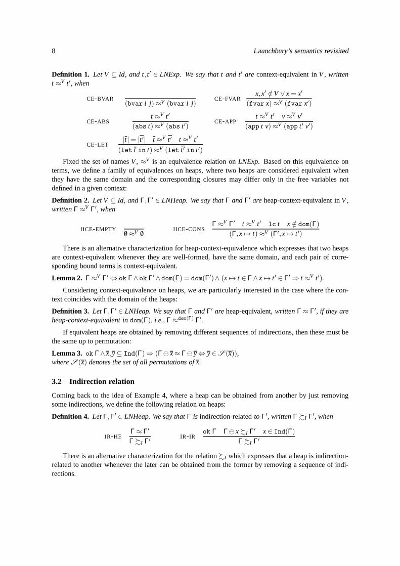
8 Launchbury’s semantics revisited
Definition 1. Let V ⊆ Id, and t, t ′ ∈ LNExp. We say that t and t′ are context-equivalent inV, writtent ≈V t ′, when
CE-BVAR(bvar i j ) ≈V (bvar i j )
CE-FVARx,x′ /∈V ∨x = x′
(fvar x) ≈V (fvar x′)
CE-ABSt ≈V t ′
(abs t) ≈V (abs t ′)CE-APP
t ≈V t ′ v≈V v′
(app t v) ≈V (app t ′ v′)
CE-LET|t| = |t ′| t ≈V t ′ t ≈V t ′
(let t in t) ≈V (let t ′ in t ′)
Fixed the set of namesV, ≈V is an equivalence relation onLNExp. Based on this equivalence onterms, we define a family of equivalences on heaps, where two heaps are considered equivalent whenthey have the same domain and the corresponding closures maydiffer only in the free variables notdefined in a given context:
Definition 2. Let V ⊆ Id, andΓ,Γ′ ∈ LNHeap. We say thatΓ andΓ′ are heap-context-equivalent inV,written Γ ≈V Γ′, when
HCE-EMPTY/0≈V /0
HCE-CONSΓ ≈V Γ′ t ≈V t ′ lc t x /∈ dom(Γ)
(Γ,x 7→ t) ≈V (Γ′,x 7→ t ′)
There is an alternative characterization for heap-context-equivalence which expresses that two heapsare context-equivalent whenever they are well-formed, have the same domain, and each pair of corre-sponding bound terms is context-equivalent.
Lemma 2. Γ ≈V Γ′ ⇔ ok Γ∧ok Γ′∧dom(Γ) = dom(Γ′)∧ (x 7→ t ∈ Γ∧x 7→ t ′ ∈ Γ′ ⇒ t ≈V t ′).
Considering context-equivalence on heaps, we are particularly interested in the case where the con-text coincides with the domain of the heaps:
Definition 3. Let Γ,Γ′ ∈ LNHeap. We say thatΓ andΓ′ are heap-equivalent, written Γ ≈ Γ′, if they areheap-context-equivalent indom(Γ), i.e.,Γ ≈dom(Γ) Γ′.
If equivalent heaps are obtained by removing different sequences of indirections, then these must bethe same up to permutation:
Lemma 3. ok Γ∧x,y⊆ Ind(Γ) ⇒ (Γ⊖x≈ Γ⊖y⇔ y∈ S (x)),whereS (x) denotes the set of all permutations ofx.
3.2 Indirection relation
Coming back to the idea of Example 4, where a heap can be obtained from another by just removingsome indirections, we define the following relation on heaps:
Definition 4. LetΓ,Γ′ ∈ LNHeap. We say thatΓ is indirection-relatedto Γ′, writtenΓ %I Γ′, when
IR-HEΓ ≈ Γ′
Γ %I Γ′ IR-IRok Γ Γ⊖x%I Γ′ x∈ Ind(Γ)
Γ %I Γ′
There is an alternative characterization for the relation%I which expresses that a heap is indirection-related to another whenever the later can be obtained from the former by removing a sequence of indi-rections.
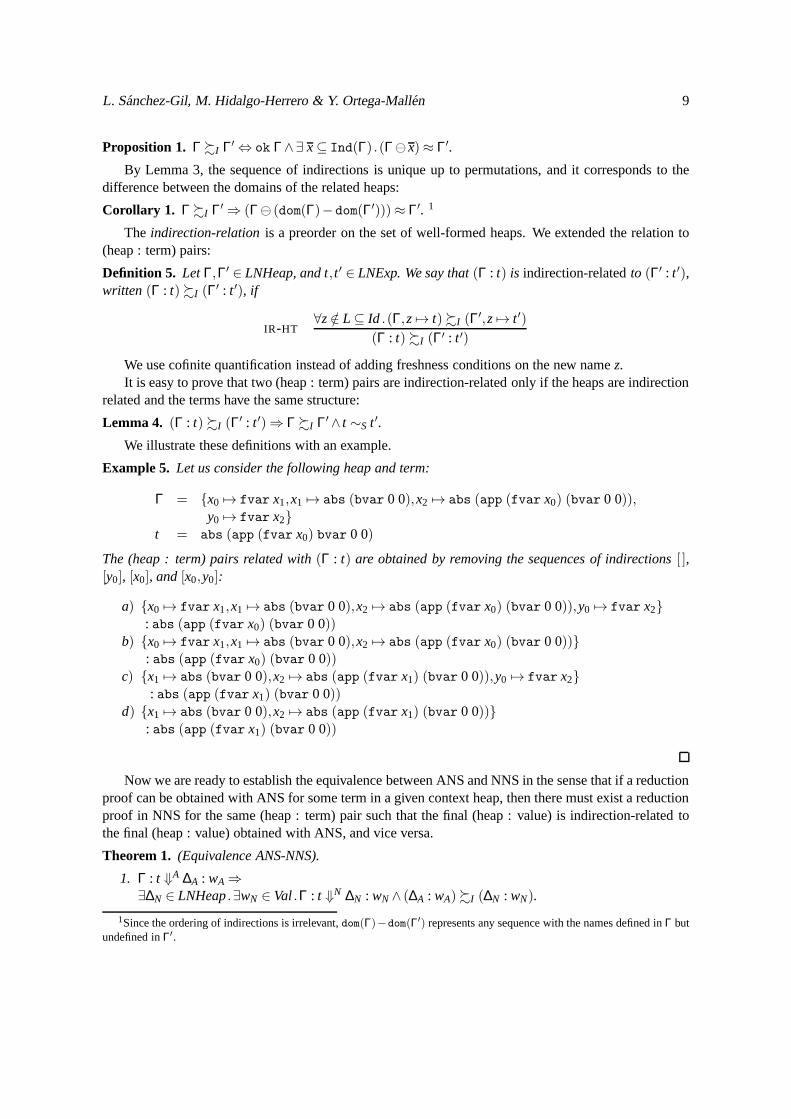
L. Sanchez-Gil, M. Hidalgo-Herrero & Y. Ortega-Mallen 9
Proposition 1. Γ %I Γ′ ⇔ ok Γ∧∃ x⊆ Ind(Γ) .(Γ⊖x) ≈ Γ′.
By Lemma 3, the sequence of indirections is unique up to permutations, and it corresponds to thedifference between the domains of the related heaps:
Corollary 1. Γ %I Γ′ ⇒ (Γ⊖ (dom(Γ)−dom(Γ′))) ≈ Γ′. 1
The indirection-relation is a preorder on the set of well-formed heaps. We extended therelation to(heap : term) pairs:
Definition 5. LetΓ,Γ′ ∈ LNHeap, and t, t ′ ∈ LNExp. We say that(Γ : t) is indirection-relatedto (Γ′ : t ′),written (Γ : t) %I (Γ′ : t ′), if
IR-HT∀z /∈ L ⊆ Id .(Γ,z 7→ t) %I (Γ′,z 7→ t ′)
(Γ : t) %I (Γ′ : t ′)
We use cofinite quantification instead of adding freshness conditions on the new namez.It is easy to prove that two (heap : term) pairs are indirection-related only if the heaps are indirection
related and the terms have the same structure:
Lemma 4. (Γ : t) %I (Γ′ : t ′) ⇒ Γ %I Γ′∧ t ∼S t ′.
We illustrate these definitions with an example.
Example 5. Let us consider the following heap and term:
Γ = {x0 7→ fvar x1,x1 7→ abs (bvar 0 0),x2 7→ abs (app (fvar x0) (bvar 0 0)),y0 7→ fvar x2}
t = abs (app (fvar x0) bvar 0 0)
The (heap : term) pairs related with(Γ : t) are obtained by removing the sequences of indirections[ ],[y0], [x0], and[x0,y0]:
a) {x0 7→ fvar x1,x1 7→ abs (bvar 0 0),x2 7→ abs (app (fvar x0) (bvar 0 0)),y0 7→ fvar x2}: abs (app (fvar x0) (bvar 0 0))
b) {x0 7→ fvar x1,x1 7→ abs (bvar 0 0),x2 7→ abs (app (fvar x0) (bvar 0 0))}: abs (app (fvar x0) (bvar 0 0))
c) {x1 7→ abs (bvar 0 0),x2 7→ abs (app (fvar x1) (bvar 0 0)),y0 7→ fvar x2}: abs (app (fvar x1) (bvar 0 0))
d) {x1 7→ abs (bvar 0 0),x2 7→ abs (app (fvar x1) (bvar 0 0))}: abs (app (fvar x1) (bvar 0 0))
Now we are ready to establish the equivalence between ANS andNNS in the sense that if a reductionproof can be obtained with ANS for some term in a given contextheap, then there must exist a reductionproof in NNS for the same (heap : term) pair such that the final (heap : value) is indirection-related tothe final (heap : value) obtained with ANS, and vice versa.
Theorem 1. (Equivalence ANS-NNS).
1. Γ : t ⇓A ∆A : wA ⇒∃∆N ∈ LNHeap.∃wN ∈ Val.Γ : t ⇓N ∆N : wN ∧ (∆A : wA) %I (∆N : wN).
1Since the ordering of indirections is irrelevant,dom(Γ)−dom(Γ′) represents any sequence with the names defined inΓ butundefined inΓ′.
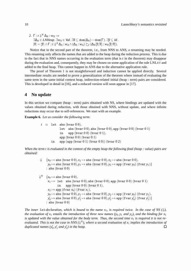
10 Launchbury’s semantics revisited
2. Γ : t ⇓N ∆N : wN ⇒∃∆A ∈ LNHeap.∃wA ∈ Val.∃x⊆ dom(∆N)−dom(Γ) .∃y⊆ Id .|x| = |y| ∧Γ : t ⇓A ∆A : wA∧ (∆A : wA) %I (∆N[y/x] : wN[y/x]).
Notice that in the second part of the theorem, i.e., from NNS to ANS, a renaming may be needed.This renaming only affects the names that are added to the heap during the reduction process. This is dueto the fact that in NNS names occurring in the evaluation term(that ist in the theorem) may disappearduring the evaluation and, consequently, they may be chosenon some application of the rule LNLET andadded to the final heap. This cannot happen in ANS due to the alternative application rule.
The proof of Theorem 1 is not straightforward and induction cannot be applied directly. Severalintermediate results are needed to prove a generalization of the theorem where instead of evaluating thesame term in the same initial context heap, indirection-related initial (heap : term) pairs are considered.This is developed in detail in [16], and a reduced version will soon appear in [17].
4 No update
In this section we compare (heap : term) pairs obtained with NS, where bindings are updated with thevalues obtained during reduction, with those obtained withNNS, without update, and where infinitereductions may occur due to self-references. We start with an example.
Example 6. Let us consider the following term:
t ≡ let abs (bvar 0 0),let abs (bvar 0 0),abs (bvar 0 0),app (bvar 0 0) (bvar 0 1)in app (bvar 0 0) (bvar 0 1),app (bvar 0 0) (bvar 0 1)
in app (app (bvar 0 1) (bvar 0 0)) (bvar 0 2)
When the term t is evaluated in the context of the empty heap the following final (heap : value) pairs areobtained:
⇓ {x0 7→ abs (bvar 0 0),x1 7→ abs (bvar 0 0),x2 7→ abs (bvar 0 0),y0 7→ abs (bvar 0 0),y1 7→ abs (bvar 0 0),y2 7→ app (fvar y0) (fvar y1)}
: abs (bvar 0 0)
⇓N {x0 7→ abs (bvar 0 0),x1 7→ let abs (bvar 0 0),abs (bvar 0 0),app (bvar 0 0) (bvar 0 1)
in app (bvar 0 0) (bvar 0 1),x2 7→ app (fvar x0) (fvar x1),y0 7→ abs (bvar 0 0),y1 7→ abs (bvar 0 0),y2 7→ app (fvar y0) (fvar y1),y′0 7→ abs (bvar 0 0),y′1 7→ abs (bvar 0 0),y′2 7→ app (fvar y′0) (fvar y′1)}
: abs (bvar 0 0)
The innerlet-declaration, which is bound to the name x1, is required twice. In the case of NS (⇓),the evaluation of x1 entails the introduction of three new names (y0,y1 and y2), and the binding for x1is updated with the value obtained for the body term. Thus, the second time x1 is required it is not re-evaluated. This is not the case in NNS (⇓N), where a second evaluation of x1 implies the introduction ofduplicated names (y′0,y
′1 and y′2) in the heap.
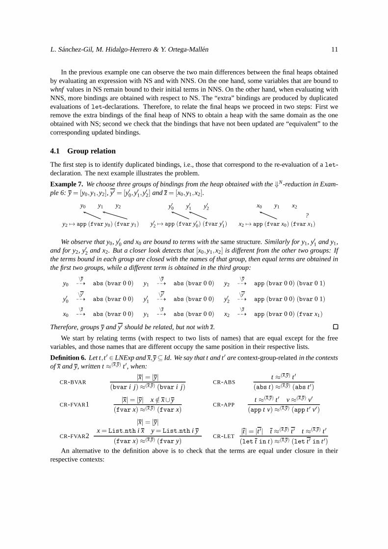
L. Sanchez-Gil, M. Hidalgo-Herrero & Y. Ortega-Mallen 11
In the previous example one can observe the two main differences between the final heaps obtainedby evaluating an expression with NS and with NNS. On the one hand, some variables that are bound towhnf values in NS remain bound to their initial terms in NNS. On theother hand, when evaluating withNNS, more bindings are obtained with respect to NS. The “extra” bindings are produced by duplicatedevaluations oflet-declarations. Therefore, to relate the final heaps we proceed in two steps: First weremove the extra bindings of the final heap of NNS to obtain a heap with the same domain as the oneobtained with NS; second we check that the bindings that havenot been updated are “equivalent” to thecorresponding updated bindings.
4.1 Group relation
The first step is to identify duplicated bindings, i.e., those that correspond to the re-evaluation of alet-declaration. The next example illustrates the problem.
Example 7. We choose three groups of bindings from the heap obtained with the⇓N-reduction in Exam-ple 6: y = [y0,y1,y2], y′ = [y′0,y
′1,y
′2] andz= [x0,y1,x2].
y2 7→ app (fvar y0) (fvar y1)
y0 y1 y2
y′2 7→ app (fvar y′0) (fvar y′1)
y′0 y′1 y′2
x2 7→ app (fvar x0) (fvar x1)
x0 y1 x2
?
We observe that y0, y′0 and x0 are bound to terms with thesame structure. Similarly for y1, y′1 and y1,and for y2, y′2 and x2. But a closer look detects that[x0,y1,x2] is different from the other two groups: Ifthe terms bound in each group are closed with the names of thatgroup, then equal terms are obtained inthe first two groups, while a different term is obtained in thethird group:
y0\y99K abs (bvar 0 0) y1
\y99K abs (bvar 0 0) y2
\y99K app (bvar 0 0) (bvar 0 1)
y′0\y′99K abs (bvar 0 0) y′1
\y′99K abs (bvar 0 0) y′2
\y′99K app (bvar 0 0) (bvar 0 1)
x0\z99K abs (bvar 0 0) y1
\z99K abs (bvar 0 0) x2
\z99K app (bvar 0 0) (fvar x1)
Therefore, groupsy andy′ should be related, but not withz.
We start by relating terms (with respect to two lists of names) that are equal except for the freevariables, and those names that are different occupy the same position in their respective lists.
Definition 6. Let t, t ′ ∈ LNExp andx,y⊆ Id. We say that t and t′ arecontext-group-relatedin the contextsof x andy, written t≈(x,y) t ′, when:
CR-BVAR|x| = |y|
(bvar i j ) ≈(x,y) (bvar i j )CR-ABS
t ≈(x,y) t ′
(abs t) ≈(x,y) (abs t ′)
CR-FVAR1|x| = |y| x /∈ x∪y
(fvar x) ≈(x,y) (fvar x)CR-APP
t ≈(x,y) t ′ v≈(x,y) v′
(app t v) ≈(x,y) (app t ′ v′)
CR-FVAR2
|x| = |y|x = List.nth i x y= List.nth i y
(fvar x) ≈(x,y) (fvar y)CR-LET
|t| = |t ′| t ≈(x,y) t ′ t ≈(x,y) t ′
(let t in t) ≈(x,y) (let t ′ in t ′)An alternative to the definition above is to check that the terms are equal under closure in their
respective contexts:
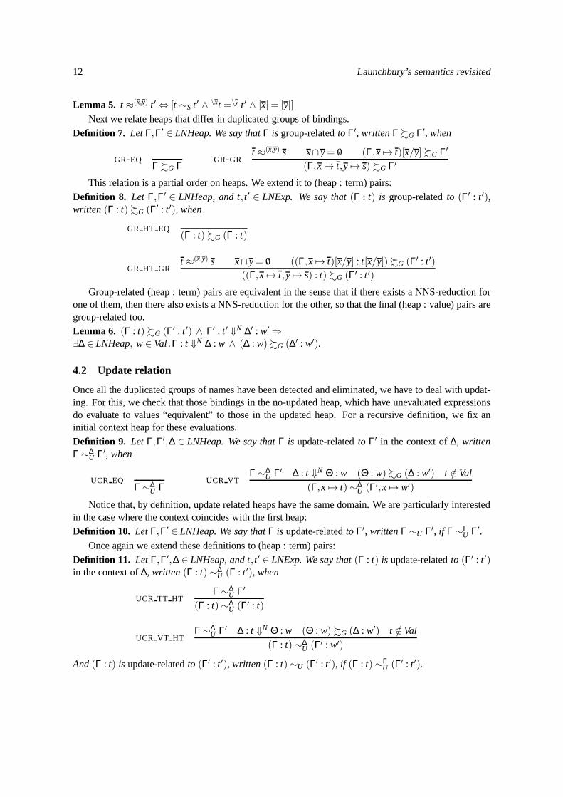
12 Launchbury’s semantics revisited
Lemma 5. t ≈(x,y) t ′ ⇔ [t ∼S t ′ ∧ \xt =\y t ′ ∧ |x| = |y|]Next we relate heaps that differ in duplicated groups of bindings.
Definition 7. LetΓ,Γ′ ∈ LNHeap. We say thatΓ is group-relatedto Γ′, writtenΓ %G Γ′, when
GR-EQΓ %G Γ
GR-GRt ≈(x,y) s x∩y = /0 (Γ,x 7→ t)[x/y] %G Γ′
(Γ,x 7→ t,y 7→ s) %G Γ′
This relation is a partial order on heaps. We extend it to (heap : term) pairs:
Definition 8. Let Γ,Γ′ ∈ LNHeap, and t, t ′ ∈ LNExp. We say that(Γ : t) is group-relatedto (Γ′ : t ′),written (Γ : t) %G (Γ′ : t ′), when
GR HT EQ(Γ : t) %G (Γ : t)
GR HT GRt ≈(x,y) s x∩y= /0 ((Γ,x 7→ t)[x/y] : t[x/y]) %G (Γ′ : t ′)
((Γ,x 7→ t,y 7→ s) : t) %G (Γ′ : t ′)
Group-related (heap : term) pairs are equivalent in the sense that if there exists a NNS-reduction forone of them, then there also exists a NNS-reduction for the other, so that the final (heap : value) pairs aregroup-related too.
Lemma 6. (Γ : t) %G (Γ′ : t ′) ∧ Γ′ : t ′ ⇓N ∆′ : w′ ⇒∃∆ ∈ LNHeap, w∈ Val.Γ : t ⇓N ∆ : w ∧ (∆ : w) %G (∆′ : w′).
4.2 Update relation
Once all the duplicated groups of names have been detected and eliminated, we have to deal with updat-ing. For this, we check that those bindings in the no-updatedheap, which have unevaluated expressionsdo evaluate to values “equivalent” to those in the updated heap. For a recursive definition, we fix aninitial context heap for these evaluations.
Definition 9. Let Γ,Γ′,∆ ∈ LNHeap. We say thatΓ is update-relatedto Γ′ in the context of∆, writtenΓ ∼∆
U Γ′, when
UCR EQΓ ∼∆
U ΓUCR VT
Γ ∼∆U Γ′ ∆ : t ⇓N Θ : w (Θ : w) %G (∆ : w′) t /∈ Val
(Γ,x 7→ t) ∼∆U (Γ′,x 7→ w′)
Notice that, by definition, update related heaps have the same domain. We are particularly interestedin the case where the context coincides with the first heap:
Definition 10. Let Γ,Γ′ ∈ LNHeap. We say thatΓ is update-relatedto Γ′, writtenΓ ∼U Γ′, if Γ ∼ΓU Γ′.
Once again we extend these definitions to (heap : term) pairs:
Definition 11. Let Γ,Γ′,∆ ∈ LNHeap, and t, t ′ ∈ LNExp. We say that(Γ : t) is update-relatedto (Γ′ : t ′)in the context of∆, written (Γ : t) ∼∆
U (Γ : t ′), when
UCR TT HTΓ ∼∆
U Γ′
(Γ : t) ∼∆U (Γ′ : t)
UCR VT HTΓ ∼∆
U Γ′ ∆ : t ⇓N Θ : w (Θ : w) %G (∆ : w′) t /∈ Val
(Γ : t) ∼∆U (Γ′ : w′)
And(Γ : t) is update-relatedto (Γ′ : t ′), written (Γ : t) ∼U (Γ′ : t ′), if (Γ : t) ∼ΓU (Γ′ : t ′).
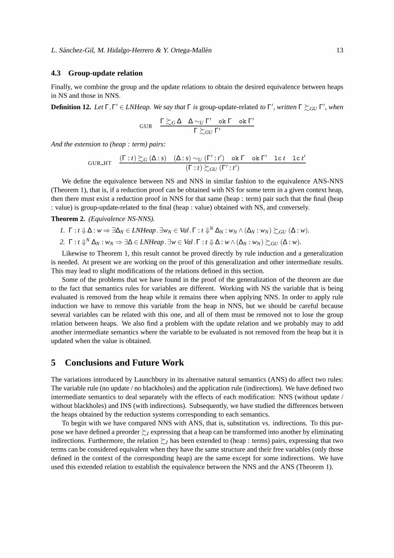
L. Sanchez-Gil, M. Hidalgo-Herrero & Y. Ortega-Mallen 13
4.3 Group-update relation
Finally, we combine the group and the update relations to obtain the desired equivalence between heapsin NS and those in NNS.
Definition 12. LetΓ,Γ′ ∈ LNHeap. We say thatΓ is group-update-relatedto Γ′, writtenΓ %GU Γ′, when
GURΓ %G ∆ ∆ ∼U Γ′ ok Γ ok Γ′
Γ %GU Γ′
And the extension to (heap : term) pairs:
GUR HT(Γ : t) %G (∆ : s) (∆ : s) ∼U (Γ′ : t ′) ok Γ ok Γ′ lc t lc t ′
(Γ : t) %GU (Γ′ : t ′)
We define the equivalence between NS and NNS in similar fashion to the equivalence ANS-NNS(Theorem 1), that is, if a reduction proof can be obtained with NS for some term in a given context heap,then there must exist a reduction proof in NNS for that same (heap : term) pair such that the final (heap: value) is group-update-related to the final (heap : value) obtained with NS, and conversely.
Theorem 2. (Equivalence NS-NNS).
1. Γ : t ⇓ ∆ : w⇒∃∆N ∈ LNHeap.∃wN ∈ Val.Γ : t ⇓N ∆N : wN ∧ (∆N : wN) %GU (∆ : w).
2. Γ : t ⇓N ∆N : wN ⇒∃∆ ∈ LNHeap.∃w∈ Val.Γ : t ⇓ ∆ : w∧ (∆N : wN) %GU (∆ : w).
Likewise to Theorem 1, this result cannot be proved directlyby rule induction and a generalizationis needed. At present we are working on the proof of this generalization and other intermediate results.This may lead to slight modifications of the relations definedin this section.
Some of the problems that we have found in the proof of the generalization of the theorem are dueto the fact that semantics rules for variables are different. Working with NS the variable that is beingevaluated is removed from the heap while it remains there when applying NNS. In order to apply ruleinduction we have to remove this variable from the heap in NNS, but we should be careful becauseseveral variables can be related with this one, and all of them must be removed not to lose the grouprelation between heaps. We also find a problem with the updaterelation and we probably may to addanother intermediate semantics where the variable to be evaluated is not removed from the heap but it isupdated when the value is obtained.
5 Conclusions and Future Work
The variations introduced by Launchbury in its alternativenatural semantics (ANS) do affect two rules:The variable rule (no update / no blackholes) and the application rule (indirections). We have defined twointermediate semantics to deal separately with the effectsof each modification: NNS (without update /without blackholes) and INS (with indirections). Subsequently, we have studied the differences betweenthe heaps obtained by the reduction systems corresponding to each semantics.
To begin with we have compared NNS with ANS, that is, substitution vs. indirections. To this pur-pose we have defined a preorder%I expressing that a heap can be transformed into another by eliminatingindirections. Furthermore, the relation%I has been extended to (heap : terms) pairs, expressing that twoterms can be considered equivalent when they have the same structure and their free variables (only thosedefined in the context of the corresponding heap) are the sameexcept for some indirections. We haveused this extended relation to establish the equivalence between the NNS and the ANS (Theorem 1).
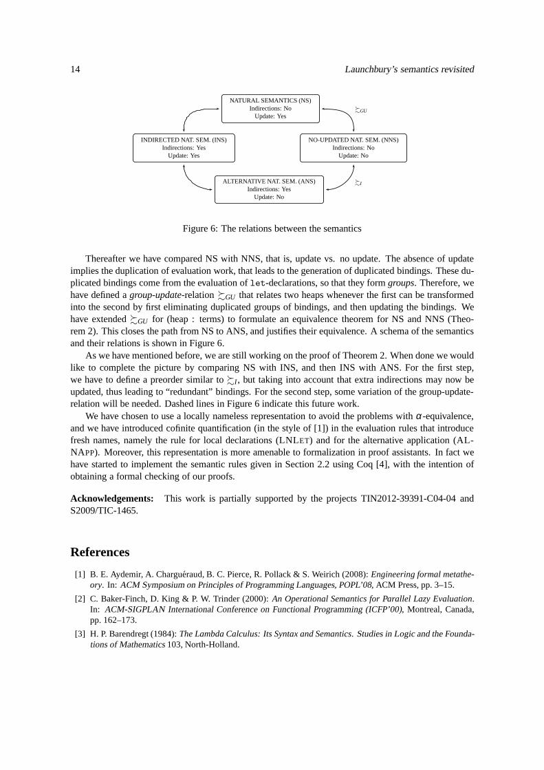
14 Launchbury’s semantics revisited
NATURAL SEMANTICS (NS)Indirections: No
Update: Yes
INDIRECTED NAT. SEM. (INS)Indirections: Yes
Update: Yes
NO-UPDATED NAT. SEM. (NNS)Indirections: No
Update: No
ALTERNATIVE NAT. SEM. (ANS)Indirections: Yes
Update: No
%I
%GU
Figure 6: The relations between the semantics
Thereafter we have compared NS with NNS, that is, update vs. no update. The absence of updateimplies the duplication of evaluation work, that leads to the generation of duplicated bindings. These du-plicated bindings come from the evaluation oflet-declarations, so that they formgroups. Therefore, wehave defined agroup-update-relation%GU that relates two heaps whenever the first can be transformedinto the second by first eliminating duplicated groups of bindings, and then updating the bindings. Wehave extended%GU for (heap : terms) to formulate an equivalence theorem for NSand NNS (Theo-rem 2). This closes the path from NS to ANS, and justifies theirequivalence. A schema of the semanticsand their relations is shown in Figure 6.
As we have mentioned before, we are still working on the proofof Theorem 2. When done we wouldlike to complete the picture by comparing NS with INS, and then INS with ANS. For the first step,we have to define a preorder similar to%I , but taking into account that extra indirections may now beupdated, thus leading to “redundant” bindings. For the second step, some variation of the group-update-relation will be needed. Dashed lines in Figure 6 indicate this future work.
We have chosen to use a locally nameless representation to avoid the problems withα-equivalence,and we have introduced cofinite quantification (in the style of [1]) in the evaluation rules that introducefresh names, namely the rule for local declarations (LNLET) and for the alternative application (AL-NAPP). Moreover, this representation is more amenable to formalization in proof assistants. In fact wehave started to implement the semantic rules given in Section 2.2 using Coq [4], with the intention ofobtaining a formal checking of our proofs.
Acknowledgements: This work is partially supported by the projects TIN2012-39391-C04-04 andS2009/TIC-1465.
References
[1] B. E. Aydemir, A. Chargueraud, B. C. Pierce, R. Pollack &S. Weirich (2008):Engineering formal metathe-ory. In: ACM Symposium on Principles of Programming Languages, POPL’08, ACM Press, pp. 3–15.
[2] C. Baker-Finch, D. King & P. W. Trinder (2000):An Operational Semantics for Parallel Lazy Evaluation.In: ACM-SIGPLAN International Conference on Functional Programming (ICFP’00), Montreal, Canada,pp. 162–173.
[3] H. P. Barendregt (1984):The Lambda Calculus: Its Syntax and Semantics. Studies in Logic and the Founda-tions of Mathematics103, North-Holland.
L. Sanchez-Gil, M. Hidalgo-Herrero & Y. Ortega-Mallen 15
[4] Y. Bertot (2006): Coq in a Hurry. CoRR abs/cs/0603118. Available athttp://arxiv.org/abs/cs/0603118.
[5] J. Breitner (2013):The Correctness of Launchbury’s Natural Semantics for LazyEvaluation. Archive of For-mal Proofs. http://afp.sf.net/entries/Launchbury.shtml, Formal proof development, Amendedversion May 2014.
[6] N. G. de Bruijn (1972):Lambda calculus notation with nameless dummies, a tool for automatic formulamanipulation, with application to the Church-Rosser theorem. Indagationes Mathematicae75(5), pp. 381–392.
[7] A. Chargueraud (2011):The Locally Nameless Representation. Journal of Automated Reasoning, pp. 1–46.
[8] M. van Eekelen & M. de Mol (2007):Reflections on Type Theory,λ -calculus, and the Mind. Essays dedi-cated to Henk Barendregt on the Occasion of his 60th Birthday, chapter Proving Lazy Folklore with MixedLazy/Strict Semantics, pp. 87–101. Radboud University Nijmegen.
[9] J. Launchbury (1993):A Natural Semantics for Lazy Evaluation. In: ACM Symp. on Principles of Program-ming Languages, POPL’93, ACM Press, pp. 144–154.
[10] K. Nakata & M. Hasegawa (2009):Small-step and big-step semantics for call-by-need. Journal of FunctionalProgramming19(6), pp. 699–722.
[11] T. Nipkow, L. C. Paulson & M. Wenzel (2002):Isabelle/HOL — A Proof Assistant for Higher-Order Logic.LNCS 2283, Springer.
[12] L. Sanchez-Gil, M. Hidalgo-Herrero & Y. Ortega-Mall´en (2010):Call-by-need, call-by-name, and naturalsemantics. Technical Report UU-CS-2010-020, Department of Information and Computing Sciences, UtrechUniversity.
[13] L. Sanchez-Gil, M. Hidalgo-Herrero & Y. Ortega-Mall´en (2010):Trends in Functional Programming, chapterAn Operational Semantics for Distributed Lazy Evaluation,pp. 65–80. 10, Intellect.
[14] L. Sanchez-Gil, M. Hidalgo-Herrero & Y. Ortega-Mall´en (2012):A locally nameless representation for a nat-ural semantics for lazy evaluation. Technical Report 01/12, Dpt. Sistemas Informaticos y Computacion. Univ.Complutense de Madrid. Http://federwin.sip.ucm.es/sic/investigacion/publicaciones/pdfs/SIC-1-12.pdf.
[15] L. Sanchez-Gil, M. Hidalgo-Herrero & Y. Ortega-Mall´en (2012):A Locally Nameless Representation for aNatural Semantics for Lazy Evaluation. In: Theoretical Aspects of Computing ICTAC 2012, LNCS 7521,Springer, p. 105119.
[16] L. Sanchez-Gil, M. Hidalgo-Herrero & Y. Ortega-Mall´en (2013):The role of indirections in lazy naturalsemantics (extended version). Technical Report 13/13, Dpt. Sistemas Informaticos y Computacion. Univ.Complutense de Madrid. Http://federwin.sip.ucm.es/sic/investigacion/publicaciones/pdfs/TR-13-13.pdf.
[17] L. Sanchez-Gil, M. Hidalgo-Herrero & Y. Ortega-Mall´en (2014):The role of indirections in lazy naturalsemantics. In: Proceedings of Ershov Informatics Conference (the PSI Conference Series, 9th edition). Toappear.
[18] P. Sestoft (1997):Deriving a lazy abstract machine. Journal of Functional Programming7(3), pp. 231–264.
[19] C. Urban, S. Berghofer & M. Norrish (2007):Barendregt’s Variable Convention in Rule Inductions. In:Proceedings of the 21st International Conference on Automated Deduction: Automated Deduction, LNCS4603, Springer-Verlag, pp. 35–50.
[20] C. Urban & C. Kaliszyk (2012):General Bindings and Alpha-Equivalence in Nominal Isabelle. LogicalMethods in Computer Science8(2:14), pp. 1–35.

266 Capıtulo B. Trabajo en progreso
Electronic Communications of the EASSTVolume X (2012)
Proceedings of theXII Spanish Conference on Progamming and Computer
Languages(PROLE’12)
A formalization in Coqof Launchbury’s natural semantics for lazy evaluation
Lidia Sanchez-Gil Mercedes Hidalgo-Herrero Yolanda Ortega-Mallen
15 pages
Guest Editors: Marıa-del-Mar GallardoManaging Editors: Tiziana Margaria, Julia Padberg, Gabriele TaentzerECEASST Home Page: http://www.easst.org/eceasst/ ISSN 1863-2122
ECEASST
A formalization in Coqof Launchbury’s natural semantics for lazy evaluation∗
Lidia Sanchez-Gil1 Mercedes Hidalgo-Herrero2 Yolanda Ortega-Mallen3
1,3Dpt. Sistemas Informaticos y Computacion, Facultad de CC. Matematicas, UniversidadComplutense de Madrid, Spain,[email protected], [email protected]
2Dpt. Didactica de las Matematicas, Facultad de Educacion, Universidad Complutense deMadrid, Spain,[email protected]
Abstract: We are working on the implementation of Launchbury’s semantics forlazy evaluation in the proof assistant Coq. We use a locally nameless representationwhere names are reserved for free variables, while bound variable names are re-placed by indices. This avoids the need ofα-conversion and Barendregt’s variableconvention, and facilitates the formalization in Coq. Simultaneous recursive localdeclarations in the calculus require the management of multibinders and the use ofmutually inductive types.
Keywords: Formalization, locally nameless representation, proof assistant, Coq,natural semantics, lazy evaluation.
1 Motivation
Call-by-needevaluation, which avoids repeated computations, is the semantic foundation forlazy functional programming languages like Haskell or Clean. Launchbury defines in [Lau93] anatural semantics for lazy evaluation where the set ofbindings, i.e., (variable, expression) pairs,is explicitly handled to make possible their sharing. To prove that this lazy semantics iscorrectandcomputationally adequatewith respect to a standard denotational semantics, Launchburydefines an alternative semantics. On the one hand, functional application is modeled denotation-ally by extending the environment with a variable bound to a value. This new variable representsthe formal parameter of the function, while the value corresponds to the actual argument. For acloser approach of this mechanism, applications are carried out in the alternative semantics byintroducing indirections instead of by performing theβ -reduction through substitution. On theother hand, the update of bindings with their computed values is an operational notion withouta denotational counterpart. Thus, the alternative semantics does no longer update bindings andbecomes acall-by-namesemantics.
Alas, the proof of the equivalence between the lazy semantics and its alternative version isdetailed nowhere, and a simple induction turns out to be insufficient. Intuitively, both reductionsystems should produce the same results, but this cannot be directly established. Values maycontain free variables that depend on the context of evaluation, which is represented by the heapof bindings. The changes introduced by the alternative semantics do deeply affect these heaps.
∗ Work partially supported by the projects TIN2009-14599-C03-01 and S2009/TIC-1465.
1 / 15 Volume X (2012)
Although indirections and “duplicated” bindings (a consequence of not updating) do not addrelevant information to the context, it is awkward to prove this fact.
We intend to prove formally the equivalence between Launchbury’s semantics and its alterna-tive version. In the usual representation of theλ -calculus, i.e., with variable names for free andbound variables, terms are identifed up toα-conversion. Dealing withα-equated terms usuallyimplies the use of Barendregt’s variable convention [Bar84] to avoid the renaming of bound vari-ables. However, the use of the variable convention in rule inductions is sometimes dubious andmay lead tofaulty results (as it is shown by Urban et al. in [UBN07]). Looking for a system ofbinding more amenable to formalization, we have chosen alocally namelessrepresentation (aspresented by Chargueraud in [Cha11]). This is a mixed notation where bound variable namesare replaced by de Bruijn indices [dB72], while free variables preserve their names. Hence,α-conversion is no longer needed and variable substitution is easily defined because there isno danger of name capture. Moreover, this representation issuitable for working with proofassistants like Coq [Ber06] or Isabelle [NPW02]. We have preferred Coq to Isabelle for our for-malization because Coq allows the definition of inductive types, that are needed for the recursivelocal declarations, while we encountered some problems when we first tried with Isabelle. Fur-thermore, Coq offers dependent types and proof by reflection, that will be helpful for our theoryand proof developments.
Our concern for reproducing and formalizing the proof of this equivalence is not arbitrary.Launchbury’s natural semantics has been cited frequently and has inspired many further worksas well as several extensions of his semantics , where the corresponding adequacy proofs havebeen obtained by just adapting Launchbury’s proof scheme. We have extended ourselves theλ -calculus with a new expression that introduces parallelismin functional applications [SHO10].
The paper is structured as follows: In Section2 we present the locally nameless representationof theλ -calculus extended with mutually recursive local declarations. In Section3, we expressLaunchbury’s semantic rules in the new style and present several properties of the reductionsystem that are useful for the equivalence proof.1 In Section4 we describe the current state ofthe implementation in Coq of this locally nameless translation of the syntax and the semantics.In Section5 we comment on some related work. In the last section we explain what we haveachieved so far and what remains to be done.
2 The locally nameless representation
The language described by Launchbury in [Lau93] is a normalizedλ -calculus extended withrecursive local declarations. We reproduce the restrictedsyntax in Figure1.a. Normalization isachieved in two steps. First anα-conversion is carried out so that all bound variables have distinctnames. In a second phase, arguments for applications are enforced to be variables. Thesestatictransformations simplify the definition of the reduction rules.
Next, we follow the methodology summarized in [Cha11]:
1. Define the syntax of the extendedλ -calculus in the locally nameless style.
2. Define the variable opening and variable closing operations.1 The “paper-and-pencil” proofs of these lemmas and other auxiliary results are detailed in [SHO12].
Proc. PROLE’12 2 / 15

ECEASST
x∈ Vare∈ Exp ::= λx.e | (e x) | x | let {xi = ei}ni=1 in e.
x∈ Id i, j ∈ Nv∈ Var ::= bvar i j | fvar xt ∈ LNExp ::= v | abs t | app t v | let {ti}ni=1 in t
(a) Restrictednamedsyntax (b) Locally nameless syntax
Figure 1: Extendedλ -calculus
3. Define the free variables and substitution functions, as well as the local closure predicate.
4. State and prove the properties of the operations on terms that are needed in the develop-ment to be accomplished.
2.1 Locally nameless syntax
The locally nameless (restricted) syntax is shown in Figure1.b. Var stands now for the setof variables, where we distinguish betweenbound variablesand free variables. The calculusincludes two binding constructions:λ -abstraction andlet-declaration. Being the latter amulti-binder, we follow Chargueraud [Cha11] and represent bound variables with two natural numbers:The first number is a de Bruijn index that counts how many binders (abstraction orlet) one needsto cross to the left to reach the corresponding binder for thevariable, while the second refers tothe position of the variable inside that binder. Abstractions are seen as multi-binders that bindonly one variable; thus, the second number should be zero. Inthe following, we will represent alist like {ti}ni=1 ast, with length|t|= n.
Example1 Let e∈ Expbe an expression in the named representation:
e≡ λz.let x1 = λy1.y1,x2 = λy2.y2,x3 = x in (z x2).
The corresponding locally nameless termt ∈ LNExpis:
t ≡ abs (let abs (bvar 0 0),abs (bvar 0 0),fvar x in app (bvar 1 0) (bvar 0 1)).
Notice thatx1 andx2 denoteα-equivalent expressions ine. This is more clearly seen int, whereboth expressions are represented with syntactically equalterms.
As bound variables are nameless, the first phase of Launchbury’s normalization is unneeded.However, application arguments are still restricted to variables.
2.2 Variable opening and variable closing
Variable openingandvariable closingare the main operations to manipulate locally namelessterms. We extend the definitions given by Chargueraud in [Cha11] to thelet-declaration.2
2 Multiple binders are defined in [Cha11]. Two constructions are given: One for non-recursive localdeclarations, andanother for mutually recursive expressions. Yet both extensions are not completely developed.
3 / 15 Volume X (2012)

{k→ x}(bvar i j ) =
{fvar (List.nth j x) if i = k∧ j < |x|bvar i j otherwise
{k→ x}(fvar x) = fvar x{k→ x}(abs t) = abs ({k+1→ x} t){k→ x}(app t v) = app ({k→ x} t) ({k→ x} v){k→ x}(let t in t) = let ({k+1→ x} t) in ({k+1→ x} t)
where{k→ x} t = List.map ({k→ x}·) t.
Figure 2: Variable opening
To explore the body of a binder (abstraction orlet), the corresponding bound variables arereplaced with fresh names. In the case ofabs t thevariable opening operationreplaces int witha (fresh) name every bound variable that refers to the outermost abstraction. Similarly, to openlet t in t we provide a list of|t| distinct fresh names to replace those bound variables that occurin t and int which refer to this particular declaration.
Variable opening is defined by means of a more general function {k→ x}t (Figure2), wherethe numberk represents the nesting level of the binder to be opened, andx is a list of pairwise-distinct identifiers inId. Since the level of the outermost binder is 0, variable opening is definedastx = {0→ x}t. We extend this operation to lists of terms:tx = List.map (·x) t.
The last definition and those in Figure2 include some operations on lists. We use an ML-likenotation. For instance,List.nth j x represents the( j + 1)th element ofx,3 andList.map f tapplies functionf to every term int. In the rest of definitions we will use similar list operations.
Example2 Consider the termabs (let bvar 0 1,bvar 1 0in app (abs bvar 2 0) (bvar 0 1)).Hence, the body of the abstraction is:
u≡ let bvar 0 1, bvar 1 0 in app (abs bvar 2 0 ) (bvar 0 1).
But then inu the bound variables referring to the outermost abstraction(shown squared) pointto nowhere. Therefore, we consideru[x] instead ofu, where
u[x] = {0→ x}(let bvar 0 1,bvar 1 0in app (abs bvar 2 0) (bvar 0 1))= let {1→ x}(bvar 0 1,bvar 1 0) in {1→ x}(app (abs bvar 2 0) (bvar 0 1))= let bvar 0 1,fvar x in app (abs {2→ x}(bvar 2 0)) (bvar 0 1)= let bvar 0 1,fvar x in app (abs fvar x) (bvar 0 1)
Inversely to variable opening, there is an operation to transform free names into bound vari-ables. Thevariable closingof t is represented by\xt, wherex is the list of names to be bound(recall that the names inx are distinct). Again, a general function{k← x}t (Figure3) is defined.Wheneverfvar x is encountered,x is looked up inx: If x occurs in positionj, then the freevariable is replaced bybvar k j, otherwise it is left unchanged. Variable closing is then definedas\xt = {0← x}t. Its extension to lists is\xt = List.map (\x·) t.
Example3 We close the term obtained by opening the body of the abstraction in Example2(i.e., the termu): t ≡ let bvar 0 1,fvar x in app (abs fvar x) (bvar 0 1).
3 In order to better accommodate to bound variables indices, elements in a list are numbered starting with 0.
Proc. PROLE’12 4 / 15
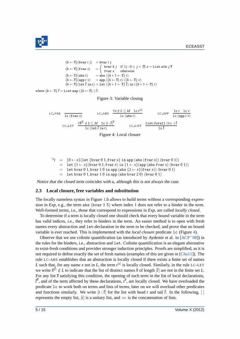
ECEASST
{k← x}(bvar i j ) = bvar i j
{k← x}(fvar x) =
{bvar k j if ∃ j : 0≤ j < |x|.x = List.nth j xfvar x otherwise
{k← x}(abs t) = abs ({k+1← x} t){k← x}(app t v) = app ({k← x} t) ({k← x} v){k← x}(let t in t) = let ({k+1← x} t) in ({k+1← x} t)
where{k← x} t = List.map ({k← x}·) t.
Figure 3: Variable closing
LC VARlc (fvar x)
LC ABS∀x /∈ L ⊆ Id lc t [x]
lc (abs t)LC APP
lc t lc vlc (app t v)
LC LET∀x|t| /∈ L⊆ Id lc [t : t]x
lc (let t in t)LC LIST
List.forall (lc ·) tlc t
Figure 4: Local closure
\xt = {0← x}(let {bvar 0 1,fvar x} in app (abs (fvar x)) (bvar 0 1))= let {1← x}(bvar 0 1,fvar x) in {1← x}(app (abs fvar x) (bvar 0 1))= let bvar 0 1,bvar 1 0in app (abs {2← x}(fvar x)) (bvar 0 1)= let bvar 0 1,bvar 1 0in app (abs bvar 2 0) (bvar 0 1)
Notice that the closed term coincides withu, although this is not always the case.
2.3 Local closure, free variables and substitution
The locally nameless syntax in Figure1.b allows to build terms without a corresponding expres-sion inExp, e.g., the termabs (bvar 1 5) where index 1 does not refer to a binder in the term.Well-formed terms, i.e., those that correspond to expressions inExp, are calledlocally closed.
To determine if a term is locally closed one should check thatevery bound variable in the termhas valid indices, i.e., they refer to binders in the term. Aneasier method is to open with freshnames every abstraction andlet-declaration in the term to be checked, and prove that no boundvariable is ever reached. This is implemented with thelocal closurepredicatelc (Figure4).
Observe that we use cofinite quantification (as introduced byAydemir et al. in [ACP+08]) inthe rules for the binders, i.e., abstraction andlet. Cofinite quantification is an elegant alternativeto exist-fresh conditions and provides stronger inductionprinciples. Proofs are simplified, as it isnot required to define exactly the set of fresh names (examples of this are given in [Cha11]). Therule LC-ABS establishes that an abstraction is locally closed if there exists a finite set of namesL such that, for any namex not in L, the termt [x] is locally closed. Similarly, in the ruleLC-LET
we writex|t| /∈ L to indicate that the list of distinct namesx of length|t| are not in the finite setL.For any listx satisfying this condition, the opening of each term in the list of local declarations,tx, and of the term affected by these declarations,tx, are locally closed. We have overloaded thepredicatelc to work both on terms and lists of terms; later on we will overload other predicatesand functions similarly. We write[t : t] for the list with headt and tail t. In the following, [ ]represents the empty list,[t] is a unitary list, and++ is the concatenation of lists.
5 / 15 Volume X (2012)
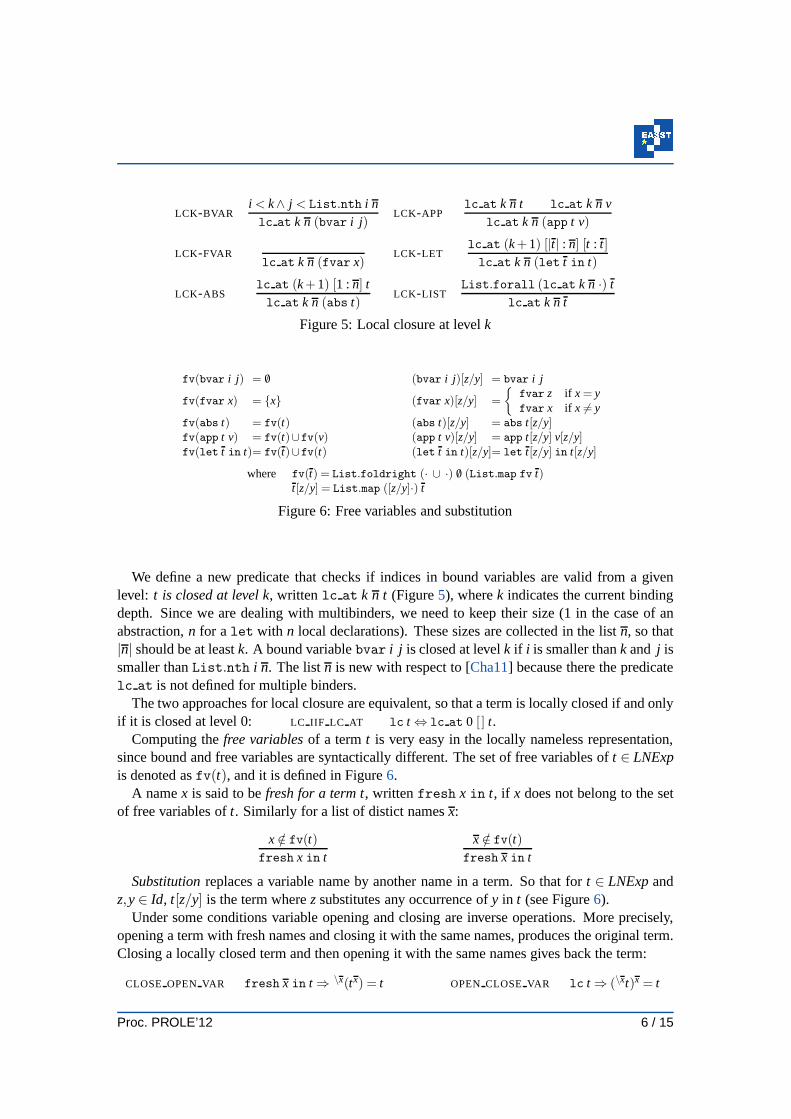
LCK-BVARi < k∧ j < List.nth i nlc at k n (bvar i j )
LCK-APPlc at k n t lc at k n v
lc at k n (app t v)
LCK-FVARlc at k n (fvar x)
LCK-LETlc at (k+1) [|t| : n] [t : t]lc at k n (let t in t)
LCK-ABSlc at (k+1) [1 : n] tlc at k n (abs t)
LCK-LISTList.forall (lc at k n ·) t
lc at k n t
Figure 5: Local closure at levelk
fv(bvar i j ) = /0 (bvar i j )[z/y] = bvar i j
fv(fvar x) = {x} (fvar x)[z/y] =
{fvar z if x = yfvar x if x 6= y
fv(abs t) = fv(t) (abs t)[z/y] = abs t[z/y]fv(app t v) = fv(t)∪fv(v) (app t v)[z/y] = app t[z/y] v[z/y]fv(let t in t)= fv(t)∪fv(t) (let t in t)[z/y]= let t[z/y] in t[z/y]
where fv(t) = List.foldright (· ∪ ·) /0 (List.map fv t)t[z/y] = List.map ([z/y]·) t
Figure 6: Free variables and substitution
We define a new predicate that checks if indices in bound variables are valid from a givenlevel: t is closed at level k, writtenlc at k n t (Figure5), wherek indicates the current bindingdepth. Since we are dealing with multibinders, we need to keep their size (1 in the case of anabstraction,n for alet with n local declarations). These sizes are collected in the listn, so that|n| should be at leastk. A bound variablebvar i j is closed at levelk if i is smaller thank and j issmaller thanList.nth i n. The listn is new with respect to [Cha11] because there the predicatelc at is not defined for multiple binders.
The two approaches for local closure are equivalent, so thata term is locally closed if and onlyif it is closed at level 0: LC IIF LC AT lc t⇔ lc at 0 [ ] t.
Computing thefree variablesof a termt is very easy in the locally nameless representation,since bound and free variables are syntactically different. The set of free variables oft ∈ LNExpis denoted asfv(t), and it is defined in Figure6.
A namex is said to befresh for a term t, writtenfresh x in t, if x does not belong to the setof free variables oft. Similarly for a list of distict namesx:
x /∈ fv(t)fresh x in t
x /∈ fv(t)fresh x in t
Substitutionreplaces a variable name by another name in a term. So that fort ∈ LNExpandz,y∈ Id, t[z/y] is the term wherezsubstitutes any occurrence ofy in t (see Figure6).
Under some conditions variable opening and closing are inverse operations. More precisely,opening a term with fresh names and closing it with the same names, produces the original term.Closing a locally closed term and then opening it with the same names gives back the term:
CLOSE OPEN VAR fresh x in t⇒ \x(tx) = t OPEN CLOSE VAR lc t⇒ (\xt)x = t
Proc. PROLE’12 6 / 15

ECEASST
LAM Γ : λx.e⇓ Γ : λx.e APPΓ : e⇓Θ : λy.e′ Θ : e′[x/y] ⇓ ∆ : w
Γ : (e x) ⇓ ∆ : w
VARΓ : e⇓ ∆ : w
(Γ,x 7→ e) : x⇓ (∆,x 7→ w) : wLET
(Γ,{xi 7→ ei}ni=1) : e⇓ ∆ : w
Γ : let {xi = ei}ni=1 in e⇓ ∆ : w
Figure 7: Natural semantics
3 Natural semantics for lazy evaluation
The natural semantics defined by Launchbury [Lau93] follows a lazy strategy. Judgements areof the formΓ : e⇓ ∆ : w, that is, the expressione∈ Exp in the context of the heapΓ reduces tothe valuew in the context of the heap∆. Values(w∈ Val) are expressions in weak-head-normal-form (whnf). Heapsare partial functions from variables into expressions. Each pair (variable,expression) is called abinding, represented byx 7→ e. During evaluation, new bindings may beadded to the heap, and bindings may be updated to their corresponding computed values. Thesemantic rules are shown in Figure7. The normalization of theλ -calculus, as mentioned inSection2, simplifies the definition of the rules, although a renaming is still needed ( ˆw in VAR) toavoid name clashing. This renaming is justified by Barendregt’s variable convention [Bar84].
Example4 Without the renaming in ruleVAR heaps may end up binding a name more thanonce. Take for instance the evaluation of the expression
e≡ let x1 = λy.(let z= λv.y in y),x2 = (x1 x3),x3 = (x1 x4),x4 = λs.sin x2
in the context of the empty heap. The evaluation ofe implies the evaluation ofx2, and then theevaluation of(x1x3). This application leads to the addition ofz 7→ λv.x3 to the heap. Eventually,the evaluation ofx3 implies the evaluation of(x1x4). Without a renaming of values, variablez isadded again to the heap, now bound toλv.x4.
Theorem 1 in [Lau93] states that “every heap/term pair occurring in the proof ofa reductionis distinctly named”, but we have found that the renaming fails to ensure this property. At least,it depends on how much fresh is this renaming.
Example5 Let us evaluate in the context of the empty heap the followingexpression:
e≡ let x1 = (x2 x3),x2 = λz.let y = λ t.t in y,x3 = λs.sin x1
{ } : e
...
LET {x1 7→ (x2 x3),x2 7→ λz.let y = λ t.t in y,x3 7→ λs.s} : x1
...
VAR {x2 7→ λz.let y = λ t.t in y,x3 7→ λs.s} : (x2 x3)
...
APP {x2 7→ λz.let y = λ t.t in y,x3 7→ λs.s} : x2
...
VAR {x3 7→ λs.s} : λz.let y = λ t.t in y
{x3 7→ λs.s} : λz.let y = λ t.t in y
LAM
At this point the VAR-rule requires to rename the value that has been obtained (which ishighlighted in the square). Notice thatx1 is fresh in the actual heap/term pair, and thus could be
7 / 15 Volume X (2012)
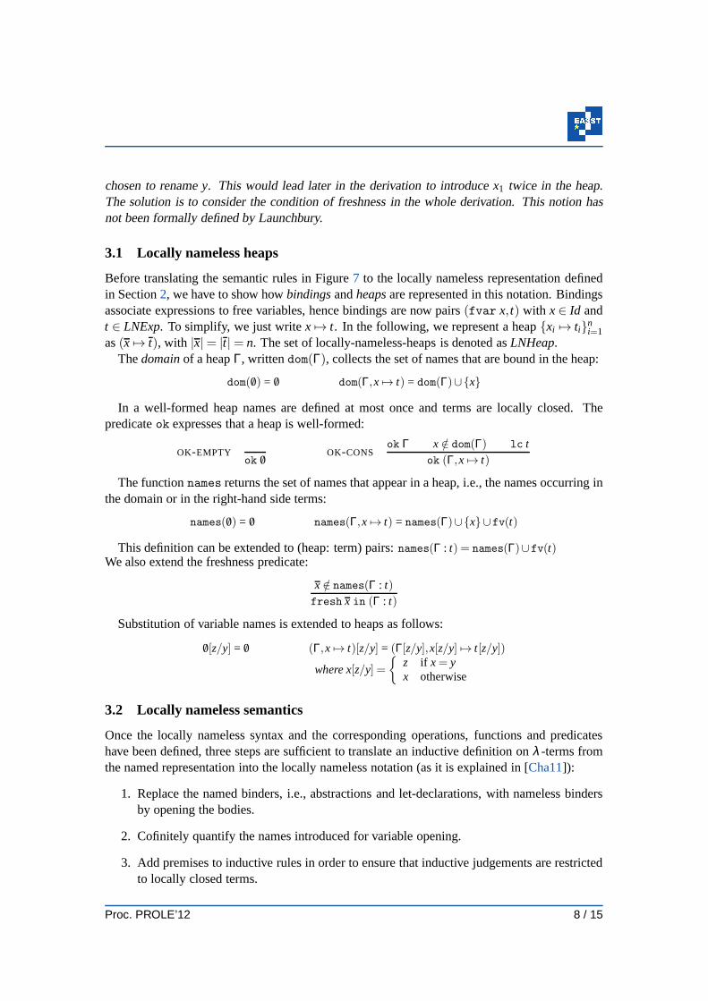
chosen to renamey. This would lead later in the derivation to introducex1 twice in the heap.The solution is to consider the condition of freshness in thewhole derivation. This notion hasnot been formally defined by Launchbury.
3.1 Locally nameless heaps
Before translating the semantic rules in Figure7 to the locally nameless representation definedin Section2, we have to show howbindingsandheapsare represented in this notation. Bindingsassociate expressions to free variables, hence bindings are now pairs(fvar x, t) with x∈ Id andt ∈ LNExp. To simplify, we just writex 7→ t. In the following, we represent a heap{xi 7→ ti}ni=1as(x 7→ t), with |x|= |t|= n. The set of locally-nameless-heaps is denoted asLNHeap.
Thedomainof a heapΓ, writtendom(Γ), collects the set of names that are bound in the heap:
dom( /0) = /0 dom(Γ,x 7→ t) = dom(Γ)∪{x}
In a well-formed heap names are defined at most once and terms are locally closed. Thepredicateok expresses that a heap is well-formed:
OK-EMPTYok /0
OK-CONSok Γ x /∈ dom(Γ) lc t
ok (Γ,x 7→ t)
The functionnames returns the set of names that appear in a heap, i.e., the namesoccurring inthe domain or in the right-hand side terms:
names( /0) = /0 names(Γ,x 7→ t) = names(Γ)∪{x}∪fv(t)
This definition can be extended to (heap: term) pairs:names(Γ : t) = names(Γ)∪fv(t)We also extend the freshness predicate:
x /∈ names(Γ : t)fresh x in (Γ : t)
Substitution of variable names is extended to heaps as follows:
/0[z/y] = /0 (Γ,x 7→ t)[z/y] = (Γ[z/y],x[z/y] 7→ t[z/y])
where x[z/y] =
{z if x = yx otherwise
3.2 Locally nameless semantics
Once the locally nameless syntax and the corresponding operations, functions and predicateshave been defined, three steps are sufficient to translate an inductive definition onλ -terms fromthe named representation into the locally nameless notation (as it is explained in [Cha11]):
1. Replace the named binders, i.e., abstractions and let-declarations, with nameless bindersby opening the bodies.
2. Cofinitely quantify the names introduced for variable opening.
3. Add premises to inductive rules in order to ensure that inductive judgements are restrictedto locally closed terms.
Proc. PROLE’12 8 / 15
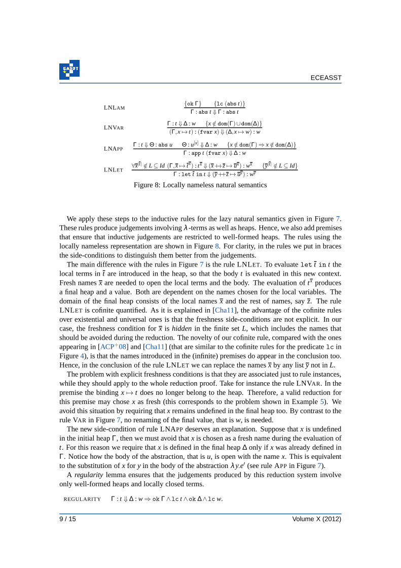
ECEASST
LNL AM{ok Γ} {lc (abs t)}
Γ : abs t ⇓ Γ : abs t
LNVARΓ : t ⇓ ∆ : w {x /∈ dom(Γ)∪dom(∆)}(Γ,x 7→ t) : (fvar x) ⇓ (∆,x 7→ w) : w
LNA PPΓ : t ⇓Θ : abs u Θ : u[x] ⇓ ∆ : w {x /∈ dom(Γ)⇒ x /∈ dom(∆)}
Γ : app t (fvar x) ⇓ ∆ : w
LNL ET∀x|t| /∈ L⊆ Id (Γ,x 7→ tx) : tx ⇓ (x++z 7→ ux) : wx {y|t| /∈ L⊆ Id}
Γ : let t in t ⇓ (y++z 7→ uy) : wy
Figure 8: Locally nameless natural semantics
We apply these steps to the inductive rules for the lazy natural semantics given in Figure7.These rules produce judgements involvingλ -terms as well as heaps. Hence, we also add premisesthat ensure that inductive judgements are restricted to well-formed heaps. The rules using thelocally nameless representation are shown in Figure8. For clarity, in the rules we put in bracesthe side-conditions to distinguish them better from the judgements.
The main difference with the rules in Figure7 is the rule LNLET. To evaluatelet t in t thelocal terms int are introduced in the heap, so that the bodyt is evaluated in this new context.Fresh namesx are needed to open the local terms and the body. The evaluation of tx producesa final heap and a value. Both are dependent on the names chosenfor the local variables. Thedomain of the final heap consists of the local namesx and the rest of names, sayz. The ruleLNL ET is cofinite quantified. As it is explained in [Cha11], the advantage of the cofinite rulesover existential and universal ones is that the freshness side-conditions are not explicit. In ourcase, the freshness condition forx is hidden in the finite setL, which includes the names thatshould be avoided during the reduction. The novelty of our cofinite rule, compared with the onesappearing in [ACP+08] and [Cha11] (that are similar to the cofinite rules for the predicatelc inFigure4), is that the names introduced in the (infinite) premises do appear in the conclusion too.Hence, in the conclusion of the rule LNLET we can replace the namesx by any listy not inL.
The problem with explicit freshness conditions is that theyare associated just to rule instances,while they should apply to the whole reduction proof. Take for instance the rule LNVAR. In thepremise the bindingx 7→ t does no longer belong to the heap. Therefore, a valid reduction forthis premise may chosex as fresh (this corresponds to the problem shown in Example5). Weavoid this situation by requiring thatx remains undefined in the final heap too. By contrast to therule VAR in Figure7, no renaming of the final value, that isw, is needed.
The new side-condition of rule LNAPP deserves an explanation. Suppose thatx is undefinedin the initial heapΓ, then we must avoid thatx is chosen as a fresh name during the evaluation oft. For this reason we require thatx is defined in the final heap∆ only if x was already defined inΓ. Notice how the body of the abstraction, that isu, is open with the namex. This is equivalentto the substitution ofx for y in the body of the abstractionλy.e′ (see rule APP in Figure7).
A regularity lemma ensures that the judgements produced by this reduction system involveonly well-formed heaps and locally closed terms.
REGULARITY Γ : t ⇓ ∆ : w⇒ ok Γ∧lc t ∧ok ∆∧lc w.
9 / 15 Volume X (2012)
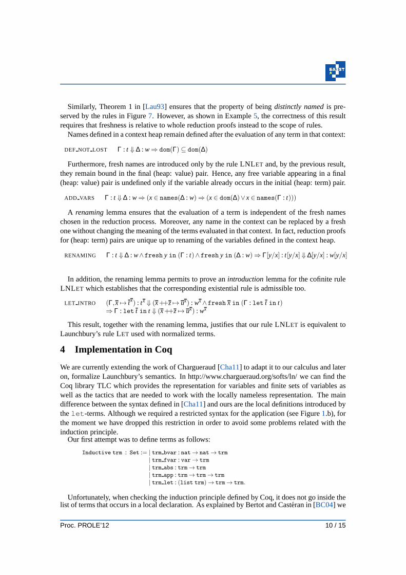
Similarly, Theorem 1 in [Lau93] ensures that the property of beingdistinctly namedis pre-served by the rules in Figure7. However, as shown in Example5, the correctness of this resultrequires that freshness is relative to whole reduction proofs instead to the scope of rules.
Names defined in a context heap remain defined after the evaluation of any term in that context:
DEF NOT LOST Γ : t ⇓ ∆ : w⇒ dom(Γ)⊆ dom(∆)
Furthermore, fresh names are introduced only by the rule LNLET and, by the previous result,they remain bound in the final (heap: value) pair. Hence, any free variable appearing in a final(heap: value) pair is undefined only if the variable already occurs in the initial (heap: term) pair.
ADD VARS Γ : t ⇓ ∆ : w⇒ (x∈ names(∆ : w)⇒ (x∈ dom(∆)∨x∈ names(Γ : t)))
A renaminglemma ensures that the evaluation of a term is independent ofthe fresh nameschosen in the reduction process. Moreover, any name in the context can be replaced by a freshone without changing the meaning of the terms evaluated in that context. In fact, reduction proofsfor (heap: term) pairs are unique up to renaming of the variables defined in the context heap.
RENAMING Γ : t ⇓ ∆ : w∧fresh y in (Γ : t)∧fresh y in (∆ : w)⇒ Γ[y/x] : t[y/x] ⇓ ∆[y/x] : w[y/x]
In addition, the renaming lemma permits to prove anintroduction lemma for the cofinite ruleLNL ET which establishes that the corresponding existential ruleis admissible too.
LET INTRO (Γ,x 7→ tx) : tx ⇓ (x++z 7→ ux) : wx∧fresh x in (Γ : let t in t)⇒ Γ : let t in t ⇓ (x++z 7→ ux) : wx
This result, together with the renaming lemma, justifies that our rule LNLET is equivalent toLaunchbury’s rule LET used with normalized terms.
4 Implementation in Coq
We are currently extending the work of Chargueraud [Cha11] to adapt it to our calculus and lateron, formalize Launchbury’s semantics. In http://www.chargueraud.org/softs/ln/ we can find theCoq library TLC which provides the representation for variables and finite sets of variables aswell as the tactics that are needed to work with the locally nameless representation. The maindifference between the syntax defined in [Cha11] and ours are the local definitions introduced bythelet-terms. Although we required a restricted syntax for the application (see Figure1.b), forthe moment we have dropped this restriction in order to avoidsome problems related with theinduction principle.
Our first attempt was to define terms as follows:
Inductive trm : Set := | trm bvar : nat→ nat→ trm
| trm fvar : var→ trm
| trm abs : trm→ trm
| trm app : trm→ trm→ trm
| trm let : (list trm)→ trm→ trm.
Unfortunately, when checking the induction principle defined by Coq, it does not go inside thelist of terms that occurs in a local declaration. As explained by Bertot and Casteran in [BC04] we
Proc. PROLE’12 10 / 15

ECEASST
have to redefine the induction principle that we want to use. To reach this objective we redefinethe terms as:
Inductive trm : Set := | trm bvar : nat→ nat→ trm
| trm fvar : var→ trm
| trm abs : trm→ trm
| trm app : trm→ trm→ trm
| trm let : L trm→ trm→ trm
with L trm := | nil Ltrm : L trm
| cons Ltrm : trm→ L trm→ L trm.
and afterward we give the following induction scheme:
Scheme trm ind2 := Induction for trm Sort Prop
with L trm ind2 := Induction for L trm Sort Prop.
We have extended the operations for variable opening and closing. To achieve this he havecompleted the recursive functions open and close at levelk. As a sample, we show here theopening at levelk. Observe how the definition of this function reproduces the two-layers structure(terms and list of terms):
Fixpoint open rec (k : nat) (vs : list var) (t : trm) {struct t} : trm :=match t with
| t bvar i j ⇒ if (andb (beq nat k i) (blt nat j (length vs)))then (t fvar(nth j vs a)) else (t bvar i j)
| t fvarx ⇒ t fvarx
| t abs t1 ⇒ t abs (open rec (S k) vs t1)| t app t1 t2 ⇒ t app (open rec k vs t1) (open rec k vs t2)| t let ts t ⇒ t let (open L rec (S k) vs ts) (open rec (S k) vs t)end
with open L rec (k : nat) (vs : list var) (ts : L trm) {struct ts} : L trm :=match ts with
| nil Lt ⇒ nil Lt
| cons Lt t ts ⇒ cons Lt (open rec k vs t) (open L rec k vs ts)end.
The functionbeq nat returns a boolean expression indicating if two given numbers are equalor not. Analogously, the functionblt nat indicates if a natural number is less or equal thanthe second one. As expected,length returns the length of a list andnth j v s areturns thej-nth element of the list vs, wherea is the default value for an index out of range. Notice thatin our definition this default value cannot be returned due tothe restrictions of the if-then-elseexpression.
Now the definition of the opening operation is:
Definition open t vs := open rec 0 vs t.
Example6 We can define the body of the abstraction given in Example2 as:
Definition body := t let (cons Lt (t bvar 0 1) (cons Lt (t bvar 1 0) (nil Lt)))(t app (t abs (t bvar 2 0)) (t bvar 0 1)).
11 / 15 Volume X (2012)

In the following lemma we prove that the opening of this term (calledbody) with a variablexcoincides with the result given previously in the example:
Lemma demo open : open body (cons x nil) = t let (cons Lt (t bvar 0 1) (cons Lt (t fvar x) nil Lt))(t app (t abs (t fvarx)) (t bvar 0 1)).
Proof.unfold body. unfold open. unfold open rec. case if. case if. unfold nth. case if. auto.Qed.
With theunfold tactic the termbody, and the functionsopen rec andnth are rewritten withtheir definitions. The tacticcase if is used to evaluateif statements. The tacticauto ends theproof automatically by applying several tactics, including reflexivity (which considers thattwo syntactically equal expressions are indeed equal).
At present we are working on the extension of the locally closed predicate, which involves thecofinite quantification over a list of identifiers (instead ofonly one identifier). We are workingon the definition of heaps and some of its predicates as well. With these definitions we will beable to prove some properties over terms and heaps.
5 Related work
In order to avoidα-conversion, we first considered a nameless representationlike the de Bruijnnotation [dB72], where variable names are replaced by natural numbers. Butthis notation hasseveral drawbacks. First of all, the de Bruijn representation is hard to read for humans. Even if weintend to check our results with a proof assistant, human readability helps intuition. Moreover,the de Bruijn notation does not have a good way to handle free variables, which are representedby indices, alike to bound variables. This is a serious weakness for our application. Launchbury’ssemantics uses context heaps that collect the bindings for the free variables that may occur in theterm under evaluation. Any change in the domain of a heap, i.e., adding or deleting a binding,would lead to a shifting of the indices, thus complicating the statement and proof of results.Therefore, we prefer the more manageable locally nameless representation, where bound variablenames are replaced by indices but free variables keep their names. This mixed notation combinesthe advantages of both named and nameless representations.On the one hand,α-conversion isavoided all the same. On the other hand, terms stay readable and easy to manipulate.
There exists in the literature different proposals for a locally nameless representation, andmany works using these representations. Chargueraud offers in [Cha11] a brief survey on theseworks, that we recommend to the interested reader.
Launchbury implicitly assumes Barendregt’s variable convention [Bar84] twice in [Lau93].First when he defines his operational semantics only for normalizedλ -terms (i.e., every binderin a term binds a distinct name, which is also distinct from any free variable); and second, whenhe requires a (fresh) renaming of the values in the rule VAR (Figure7). Urban, Berghofer andNorrish propose in [UBN07] a method to strengthen an induction principle (corresponding tosome inductive relation), so that the variable convention comes already built in the principle. Un-fortunately, we cannot apply these ideas to Launchbury’s semantics, because the semantic rulesdo not satisfy the conditions that guarantee thevariable convention compatibility, as described
Proc. PROLE’12 12 / 15
ECEASST
in [UBN07]. In fact, as we have already pointed out, Launchbury’s Theorem 1 (in [Lau93]) iscorrect only if the renaming required in each application ofthe rule VAR is fresh in the wholereduction proof. Therefore, we cannot use directly Urban’snominal package for Isabelle/HOL[Urb08] (including the recent extensions for general bindings described in [UK10]).
Nevertheless, Urban et al. achieve the “inclusion” of the variable convention in an inductionprinciple by adding to each induction rule a side condition which expresses that the set ofboundvariables (those that appear in a binding position in the rule) are fresh in someinduction context([UBN07]). Furthermore, this context is required to be finitely supported. This is closely relatedto the cofinite quantification that we have used for the rule LNLET in Figure 8. Besides, acondition to ensure the variable convention compatibilityis theequivarianceof the functionsand predicates occurring in the induction rules. Equivariance is a notion from nominal logic[Pit03]. A relation is equivariant if it is preserved by permutation of names. Although we havenot proven that the reduction relation defined by the rules inFigure8 is equivariant, ourrenaminglemmaestablishes a similar result, that is, the reduction relation is preserved by (fresh) renaming.
Nowadays there is a wide range of proof checkers and theorem provers. Wiedijk has compiledin http://www.cs.ru.nl/ freek/digimath/ a large list of these computer systems, classified by anumber of categories. Focusing in proof assistants, Barendregt and Geuvers give in [BG01] aninteresting discussion and comparison of the most widely-known proof assistants, that it is stilleffective. We also recommend the lecture of the paper by Geuvers [Geu09] on the main conceptsand history of proof assistants. We have already commented in the introduction our reasons forusing Coq [Ber06], that is, dependent and inductive types, tactics, and proof by reflection.
6 Present and future
We have used a more modern approach to binding, i.e., a locally nameless representation forthe λ -calculus extended with mutually recursive local declarations. With this representationthe reduction rule for local declarations implies the introduction of fresh names. We have usedneither an existential nor a universal rule for this case. Instead, we have opted for a cofinite ruleas introduced by Aydemir et al. in [ACP+08]. Freshness conditions are usually considered ineach rule individually. Nevertheless, this technique produces name clashing when consideringwhole reduction proofs. A solution might be to decorate judgements with the set of forbiddennames and indicate how to modify this set during the reduction process (this approach has beentaken by Sestoft in [Ses97]). However, this could be too restrictive in many occasions. Besides,existential rules are not easy to deal with because each reduction is obtained just for one specificlist of names. If any of the names in this list causes a name clashing with other reduction proofs,then it is cumbersome to demonstrate that an alternative reduction for a fresh list does exist.Cofinite quantification solves this problem because in a single step reductions are guaranteed foran infinite number of lists of names. Nonetheless, our (LET INTRO) lemma guarantees that amore conventional exists-fresh rule is correct in our reduction system too.
The cofinite quantification that we have used in our semantic rules is more complex than thosein [ACP+08] and [Cha11]. The cofinite rule LNLET in Figure8 introduces quantified variablesin the conclusion as well, as the latter depends on the chosennames.
Compared to Launchbury’s semantic rules, our locally nameless rules include several extra
13 / 15 Volume X (2012)
side-conditions. Some of these require that heaps and termsare well-formed (e.g., in LNLAM ).Others express restrictions on the choice of fresh names, sothat together with the cofinite quan-tification, fix the problem with the renaming in rule VAR that we have shown in Example5.
Our locally nameless semantics satisfies aregularity lemmawhich ensures that every term andheap involved in a reduction proof is well-formed, and arenaming lemmawhich indicates thatthe choice of names (free variables) is irrelevant as long asthey are fresh enough. A heap maybe seen as a multiple binder. Actually, the names defined (bound) in a heap can be replaced byother names, provided that terms keep their meaning in the context represented by the heap. Ourrenaming lemma ensures that whenever a heap is renamed with fresh names, reduction proofsare preserved. This renaming lemma is essential in rule induction proofs for some propertiesof the reduction system. More concretely, when one combinesseveral reduction proofs comingfrom two or more premises in a reduction rule (for instance, in rule LNAPP in Figure8).
So far, our contributions comprises the following:
1. A locally nameless representation of aλ -calculus with recursive local declarations;
2. A locally nameless version of Launchbury’s natural semantics for lazy evaluation;
3. A new version of cofinite rules where the variables quantified in the premises do appear inthe conclusion too;
4. A way to guarantee Barendregt’s variable convention by redefining Launchbury’s semanticrules with cofinite quantification and extra side-conditions;
5. A set of interesting properties of our reduction system, including the regularity, the intro-duction and the renaming lemmas; and
6. An ongoingimplementation in Coq of Launchbury’s semantics.
In the future we will use the implementation in Coq to prove formally the equivalence ofLaunchbury’s natural semantics with the alternative version given also in [Lau93]. As we men-tioned in Section1, this alternative version differs from the original one in the introduction ofindirections duringβ -reduction and the elimination of updates. We have already started withthe definition (using the locally nameless representation)of two intermediate semantics, one in-troducing indirections and the other without updates. We are investigating equivalence relationsbetween heaps obtained by each semantics, which makes able to prove the equivalence of theoriginal natural semantics and the alternative semantics through these intermediate semantics.
References
[ACP+08] B. E. Aydemir, A. Chargueraud, B. C. Pierce, R. Pollack,S. Weirich. Engineeringformal metatheory. InACM Symposium on Principles of Programming Languages(POPL’08). Pp. 3–15. ACM Press, 2008.
[Bar84] H. P. Barendregt.The Lambda Calculus: Its Syntax and Semantics. Studies in Logicand the Foundations of Mathematics 103. North-Holland, 1984.
[BC04] Y. Bertot, P. Casteran.Interactive Theorem Proving and Program Development. Coq’Art: The Calculus of Inductive Constructions. Texts in Theoretical Computer Sci-ence. Springer Verlag, 2004.
Proc. PROLE’12 14 / 15
ECEASST
[Ber06] Y. Bertot. Coq in a Hurry.CoRRabs/cs/0603118, 2006.
[BG01] H. Barendregt, H. Geuvers. Proof-assistants using dependent type systems. In Robin-son and Voronkov (eds.),Handbook of automated reasoning. Pp. 1149–1238. Else-vier Science Publishers B. V., 2001.
[dB72] N. G. de Bruijn. Lambda calculus notation with nameless dummies, a tool for auto-matic formula manipulation, with application to the Church-Rosser theorem.Inda-gationes Mathematicae75(5):381–392, 1972.
[Cha11] A. Chargueraud. The Locally Nameless Representation. Journal of Automated Rea-soning, pp. 1–46, 2011.
[Geu09] H. Geuvers. Proof assistants: History, ideas and future.Sadhana34(1):3–25, 2009.
[Lau93] J. Launchbury. A Natural Semantics for Lazy Evaluation. In ACM Symposium onPrinciples of Programming Languages (POPL’93). Pp. 144–154. ACM Press, 1993.
[NPW02] T. Nipkow, L. C. Paulson, M. Wenzel.Isabelle/HOL — A Proof Assistant for Higher-Order Logic. LNCS 2283. Springer, 2002.
[Pit03] A. M. Pitts. Nominal logic, a first order theory of names and binding.Informationand Computation186(2):165–193, 2003.
[Ses97] P. Sestoft. Deriving a lazy abstract machine.Journal of Functional Programming7(3):231–264, 1997.
[SHO10] L. Sanchez-Gil, M. Hidalgo-Herrero, Y. Ortega-Mallen. Trends in Functional Pro-gramming. Volume 10, chapter An Operational Semantics for Distributed Lazy Eval-uation, pp. 65–80. Intellect, 2010.
[SHO12] L. Sanchez-Gil, M. Hidalgo-Herrero, Y. Ortega-Mallen. A locally nameless repre-sentation for a natural semantics for lazy evaluation. Technical report 01/12, Dpt.Sistemas Informaticos y Computacion. Universidad Complutense de Madrid, 2012.http://maude.sip.ucm.es/eden-semantics/.
[UBN07] C. Urban, S. Berghofer, M. Norrish. Barendregt’s Variable Convention in Rule Induc-tions. InProceedings of the 21st International Conference on Automated Deduction:Automated Deduction. Pp. 35–50. Springer-Verlag, 2007.
[UK10] C. Urban, C. Kaliszyk. General Bindings and Alpha-Equivalence in Nominal Is-abelle. InProceedings of the 20th European Symposium on Programming. Pp. 480–500. Springer-Verlag, 2011.
[Urb08] C. Urban. Nominal Techniques in Isabelle/HOL.Journal of Automatic Reasoning40(4):327–356, 2008.
15 / 15 Volume X (2012)