projeto completo da linha de eixo 2012 rollpad
DESCRIPTION
proTRANSCRIPT

Pág 1 de 1
Escuela Universitaria de
Ingeniería Técnica Naval
C.A.S.E.M.
Pol. Río San Pedro
11510 Puerto Real (Cádiz)
Tel. 956016046. Fax. 956016045
AVISO IMPORTANTE:
El único responsable del contenido de este proyecto es el alumno que lo ha realizado. La Universidad de Cádiz, La Escuela Universitaria de Ingeniería Técnica Naval, los Departamentos a los que pertenecen el profesor tutor y los miembros del Tribunal de Proyectos Fin de Carrera así como el mismo profesor tutor NO SON RESPONSABLES DEL CONTENIDO DE ESTE PROYECTO. Los proyectos fin de carrera pueden contener errores detectados por el Tribunal de Proyectos Fin de Carrera y que estos no hayan sido implementados o corregidos en la versión aquí expuesta. La calificación de los proyectos fin de carrera puede variar desde el aprobado (5) hasta la matrícula de honor (10), por lo que el tipo y número de errores que contienen puede ser muy diferentes de un proyecto a otro. Este proyecto fin de carrera está redactado y elaborado con una finalidad académica y nunca se deberá hacer uso profesional del mismo, ya que puede contener errores que podrían poner en peligro vidas humanas.
Fdo. La Comisión de Proyectos de Fin de Carrera Escuela Universitaria de Ingeniería Técnica Naval
Universidad de Cádiz
DISEÑO DEL SISTEMA DE TRANSMISIÓN DE POTENCIA DE UN BUQUE ROPAX CON PROPULSIÓN CODAD (4 MOTORES DE 3360 BKW, 2 LÍNEAS DE EJES, 21 NUDOS Y 2500 TONS DE DESPLAZAMIENTO)
ÍNDICE
E.U.I.T. OCT-11 i
CAPÍTULO 1. INTRODUCCIÓN.......................................................................................... 1
1.1. DEFINICIÓN DE RO-PAX ........................................................................................... 1
1.2. OBJETO DEL PROYECTO........................................................................................... 2
1.3. REFERENCIAS TÉCNICAS DE LA PLATAFORMA ................................................ 3
1.4. SOCIEDAD DE CLASIFICACIÓN .............................................................................. 4
CAPÍTULO 2. DATOS FUNCIONALES DE DISEÑO ....................................................... 5
2.1. REFERENCIAS DE EQUIPOS Y ELEMENTOS MECÁNICOS ................................ 5
2.1.1. Motores propulsores ............................................................................................. 5
2.1.2. Reductor................................................................................................................ 8
2.1.3. Líneas de ejes ...................................................................................................... 10
2.1.4. Acoplamientos..................................................................................................... 11
2.1.5. Cojinetes de apoyo de los ejes ............................................................................ 11
2.1.6. Sellos del tubo de bocina..................................................................................... 11
2.1.7. Pasamamparo estanco del eje............................................................................. 11
2.1.8. Tubo de Bocina ................................................................................................... 11
2.1.9. Hélice .................................................................................................................. 12
2.1.10. Cálculo curva de potencia .................................................................................. 12
CAPÍTULO 3. DIÁMETRO DEL EJE POR CÁLCULO DIRECTO .............................. 17
3.1. CÁLCULO MOMENTO TORSOR ............................................................................. 17
3.2. TENSIÓN CORTANTE MÁXIMA............................................................................. 18
3.3. DIÁMETRO EXTERIOR DEL EJE ............................................................................ 18
3.4. REGLA DEL 30% (σELAST) Ó 18% (σMÁX.) ................................................................. 18
3.5. MOMENTO FLECTOR............................................................................................... 19
3.6. PESO DEL EJE POR METRO LINEAL ..................................................................... 19
3.7. DISTANCIA ENTRE APOYOS DEL EJE.................................................................. 20
CAPÍTULO 4. DIMENSIONAMIENTO DE LA LÍNEA DE EJES POR LA LLOYD`S
NAVAL 23
DISEÑO DEL SISTEMA DE TRANSMISIÓN DE POTENCIA DE UN BUQUE ROPAX CON PROPULSIÓN CODAD (4 MOTORES DE 3360 BKW, 2 LÍNEAS DE EJES, 21 NUDOS Y 2500 TONS DE DESPLAZAMIENTO)
ÍNDICE
E.U.I.T. OCT-11 ii
4.1. DATOS DE PARTIDA ................................................................................................ 23
4.2. CÁLCULO DEL DIÁMETRO MÍNIMO EXTERIOR DE LOS EJES ....................... 24
4.3. COMPROBACIÓN DE LOS DIÁMETROS FINALES.............................................. 25
CAPÍTULO 5. SEPARACIÓN MÁXIMA ENTRE APOYOS DE LOS EJES................. 29
5.1. SEPARACIÓN MÁXIMA ENTRE APOYOS ............................................................ 29
5.1.1. Cálculo de la distancia máxima del eje de proa ................................................. 31
5.1.2. Cálculo de la distancia máxima del eje intermedio ............................................ 31
5.1.3. Cálculo de la distancia máxima del eje de cola .................................................. 31
5.2. SITUACIÓN DE LOS APOYOS................................................................................ 32
5.3. COMPROBACIÓN DISTANCIA FINAL................................................................... 32
5.3.1. Requisitos de vibración de Whirling ................................................................... 33
5.3.2. Tensión combinada del acero del eje .................................................................. 33
5.4. COMPROBACIÓN DE LA FRECUENCIA NATURAL A TRAVÉS DE BUREAU
VERITAS 36
5.5. CÁLCULO DE VIBRACIÓN AXIAL POR LLOYD`S REGISTER.......................... 38
CAPÍTULO 6. CÁLCULO DE LAS UNIONES DE LOS EJES DE LA TRANSMISIÓN43
6.1. TIPOS DE ACOPLAMIENTOS .................................................................................. 44
6.1.1. Acoplamientos Rígidos........................................................................................ 44
6.1.2. Acoplamientos flexibles....................................................................................... 44
6.1.3. Acoplamientos torsioelásticos............................................................................. 45
6.2. TIPOS DE UNIONES BASADAS EN EL EFECTO DE FORMA ............................. 45
6.2.1. Unión Estriada.................................................................................................... 45
6.2.2. Por inserción de elementos de bloqueo............................................................... 46
6.2.2.1. Unión de bridas empernadas ........................................................................................46
6.2.2.2. Uniones de chavetas.....................................................................................................47
6.2.3. Por la acción de fuerzas de rozamiento .............................................................. 47
6.2.3.1. Unión de interferencia..................................................................................................47
6.2.3.2. Unión de interferencia hidráulica.................................................................................48
DISEÑO DEL SISTEMA DE TRANSMISIÓN DE POTENCIA DE UN BUQUE ROPAX CON PROPULSIÓN CODAD (4 MOTORES DE 3360 BKW, 2 LÍNEAS DE EJES, 21 NUDOS Y 2500 TONS DE DESPLAZAMIENTO)
ÍNDICE
E.U.I.T. OCT-11 iii
6.3. SELECCIÓN DE LAS DISTINTAS UNIONES ......................................................... 50
6.3.1. Unión eje/eje ....................................................................................................... 51
6.3.1.1. Tramo de proa a tramo intermedio...............................................................................51
6.3.1.2. Tramo intermedio a tramo de cola ...............................................................................52
6.3.2. Unión eje/reductor .............................................................................................. 52
6.3.3. Acoplamiento entre motor propulsor y reductor................................................. 53
CAPÍTULO 7. CÁLCULO DE LA UNIÓN EMPERNADA.............................................. 55
7.1. DATOS DE LA BRIDA DEL REDUCTOR................................................................ 55
7.2. DIMENSIONES DE LA ARANDELA SEGÚN ISO 7089 ......................................... 55
7.3. DIMENSIONES DE LA TUERCA SEGÚN ISO 4032 ............................................... 56
7.4. CÁLCULOS POR SOCIEDAD DE CLASIFICACIÓN.............................................. 57
7.4.1. Diámetro mínimo de los pernos .......................................................................... 57
7.4.2. Espesor mínimo de la brida ................................................................................ 58
7.5. CÁLCULO DE LA LONGITUD TOTAL DEL PERNO ............................................ 58
7.6. CÁLCULOS DIRECTOS............................................................................................. 60
7.6.1. Diámetro de los pernos de la brida..................................................................... 60
7.6.2. Espesor mínimo de la brida ................................................................................ 63
7.6.2.1. Análisis a esfuerzo cortante .........................................................................................63
7.6.2.2. Análisis a esfuerzo normal ...........................................................................................64
CAPÍTULO 8. CÁLCULO DE LA SITUACIÓN DE LOS APOYOS .............................. 67
8.1. DATOS DE PARTIDA PARA TRABAJAR CON SOFTWARE ............................... 67
8.1.1. Cargas distribuidas por metro ............................................................................ 68
8.1.1.1. Acoplamientos .............................................................................................................68
8.1.1.2. Tramo de ejes...............................................................................................................68
8.1.2. Cagas puntuales.................................................................................................. 68
8.1.3. Área de las secciones .......................................................................................... 68
8.1.3.1. Segmentos de los ejes ..................................................................................................68
8.1.3.2. Segmentos de los acoplamientos..................................................................................68
DISEÑO DEL SISTEMA DE TRANSMISIÓN DE POTENCIA DE UN BUQUE ROPAX CON PROPULSIÓN CODAD (4 MOTORES DE 3360 BKW, 2 LÍNEAS DE EJES, 21 NUDOS Y 2500 TONS DE DESPLAZAMIENTO)
ÍNDICE
E.U.I.T. OCT-11 iv
8.1.4. Momento de inercia ............................................................................................ 69
8.1.4.1. Segmentos de los ejes ..................................................................................................69
8.1.4.2. Segmentos de los acoplamientos..................................................................................69
8.1.5. Módulo de elasticidad del acero (E) ................................................................... 69
8.1.6. Densidad del acero (ρ)........................................................................................ 69
8.1.7. Distancia entre los apoyos .................................................................................. 69
8.2. DATOS OBTENIDO CON EL SOFTWARE.............................................................. 70
8.2.1. Reacciones en los apoyos.................................................................................... 71
8.2.2. Esfuerzos cortantes máximos y mínimos............................................................. 72
8.2.3. Momentos máximos y mínimos............................................................................ 72
8.2.4. Flexión máxima y mínima ................................................................................... 72
8.3. COMPROBACIÓN POR CÁLCULO DIRECTO CON LOS DATOS OBTENIDOS 72
CAPÍTULO 9. ELECCIÓN DE LOS APOYOS Y SELLOS DE BOCINA...................... 75
9.1. APOYOS ...................................................................................................................... 75
9.2. CÁLCULO DE LOS COJINETES DE LOS APOYOS ............................................... 77
9.2.1. Cojinete del primer apoyo (popa del tubo de bocina)......................................... 79
9.2.2. Cojinete del segundo apoyo ................................................................................ 79
9.2.3. Cojinete del tercer apoyo .................................................................................... 80
9.2.4. Cojinete del cuarto apoyo (proa del tubo de bocina).......................................... 81
9.2.5. Cojinete del apoyo intermedio (cámara de máquinas) ....................................... 81
9.3. SELLOS DE BOCINA................................................................................................. 83
9.4. PASAMAMPARO ESTANCO DEL EJE.................................................................... 83
BIBLIOGRAFIA ........................................................................................................................ 85
SOFTWARE UTILIZADOS ............................................................................................................. 85
PÁGINAS WEB CONSULTADAS................................................................................................... 85
ANEXO ........................................................................................................................ 87
DISEÑO DEL SISTEMA DE TRANSMISIÓN DE POTENCIA DE UN BUQUE ROPAX CON PROPULSIÓN CODAD (4 MOTORES DE 3360 BKW, 2 LÍNEAS DE EJES, 21 NUDOS Y 2500 TONS DE DESPLAZAMIENTO)
ÍNDICE FIGURAS Y TABLAS
E.U.I.T. OCT-11 v
Figura1. 1 Rampa de popa ................................................................................................1
Figura1. 2 Rampa de proa.................................................................................................2
Figura 2. 1 Dimensiones del motor .....................................................................................6
Tabla: 2.1 Dimensiones principales del motor......................................................................6
Figura 2. 2 Curva del motor para hélice paso variable ..........................................................7
Figura 2. 3 Dimensiones mín. entre motores paralelos y mamparos adyacentes .......................8
Figura 2. 4 Caja reductora ................................................................................................9
Figura 2. 5 Configuración de los ejes y los motores.............................................................10
Tabla 2.2 Potencia absorbida al 85 % y 100 % ..................................................................14
Figura 2. 6 Curva demanda de potencia del consumidor .....................................................15
Figura 3. 1 Viga Biapoyada .............................................................................................20
Tabla 4. 1 Diámetro de los ejes.........................................................................................25
Tabla 5. 1 tabla de los armónicos para una viga en distintas situaciones................................37
Tabla 5. 2 Frecuencia en Hz y rpm para los distintos armónicos ..........................................38
Figura 6. 1 Unión estriada ...............................................................................................46
Figura 6. 2 Bridas empernadas ........................................................................................46
Figura 6. 3 Unión enchavetada.........................................................................................47
Figura 6. 4 Unión por interferencia ..................................................................................48
Figura 6. 5 Unión por interferencia hidráulica...................................................................49
Figura 7. 1 Arandela ISO 7089 ........................................................................................55
Tabla 7. 1 Dimensiones arandela 64 HV 200 ......................................................................56
Figura 7. 2 Tuerca ISO 4032............................................................................................56
Figura 7. 3 Perno ISO 4014 .............................................................................................60
Tabla 7. 2 Dimensiones M64××××260-8.8................................................................................60
DISEÑO DEL SISTEMA DE TRANSMISIÓN DE POTENCIA DE UN BUQUE ROPAX CON PROPULSIÓN CODAD (4 MOTORES DE 3360 BKW, 2 LÍNEAS DE EJES, 21 NUDOS Y 2500 TONS DE DESPLAZAMIENTO)
ÍNDICE FIGURAS Y TABLAS
E.U.I.T. OCT-11 vi
Figura 7. 4 Sección crítica de la brida ...............................................................................63
Figura 8. 1 Distancia entre apoyos....................................................................................69
Figura 8. 2 Datos introducidos en el software ....................................................................70
Figura 8. 3 Diagramas de cortante, momentos y flecha .......................................................71
Tabla 8. 1 Reacciones en los distintos apoyos .....................................................................71
Figura 9. 1 Presión de trabajo cojinete..............................................................................78
Tabla 9. 1 Longitud cojinetes...........................................................................................82
DISEÑO DEL SISTEMA DE TRANSMISIÓN DE POTENCIA DE UN BUQUE ROPAX CON PROPULSIÓN CODAD (4 MOTORES DE 3360 BKW, 2 LÍNEAS DE EJES, 21 NUDOS Y 2500 TONS DE DESPLAZAMIENTO)
CAPÍTULO 1: INTRODUCCIÓN
E.U.I.T OCT-11 1
CAPÍTULO 1. INTRODUCCIÓN
1.1. DEFINICIÓN DE RO-PAX
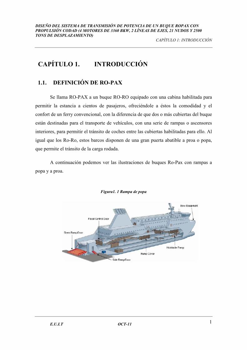
Se llama RO-PAX a un buque RO-RO equipado con una cabina habilitada para
permitir la estancia a cientos de pasajeros, ofreciéndole a éstos la comodidad y el
confort de un ferry convencional, con la diferencia de que dos o más cubiertas del buque
están destinadas para el transporte de vehículos, con una serie de rampas o ascensores
interiores, para permitir el tránsito de coches entre las cubiertas habilitadas para ello. Al
igual que los Ro-Ro, estos barcos disponen de una gran puerta abatible a proa o popa,
que permite el tránsito de la carga rodada.
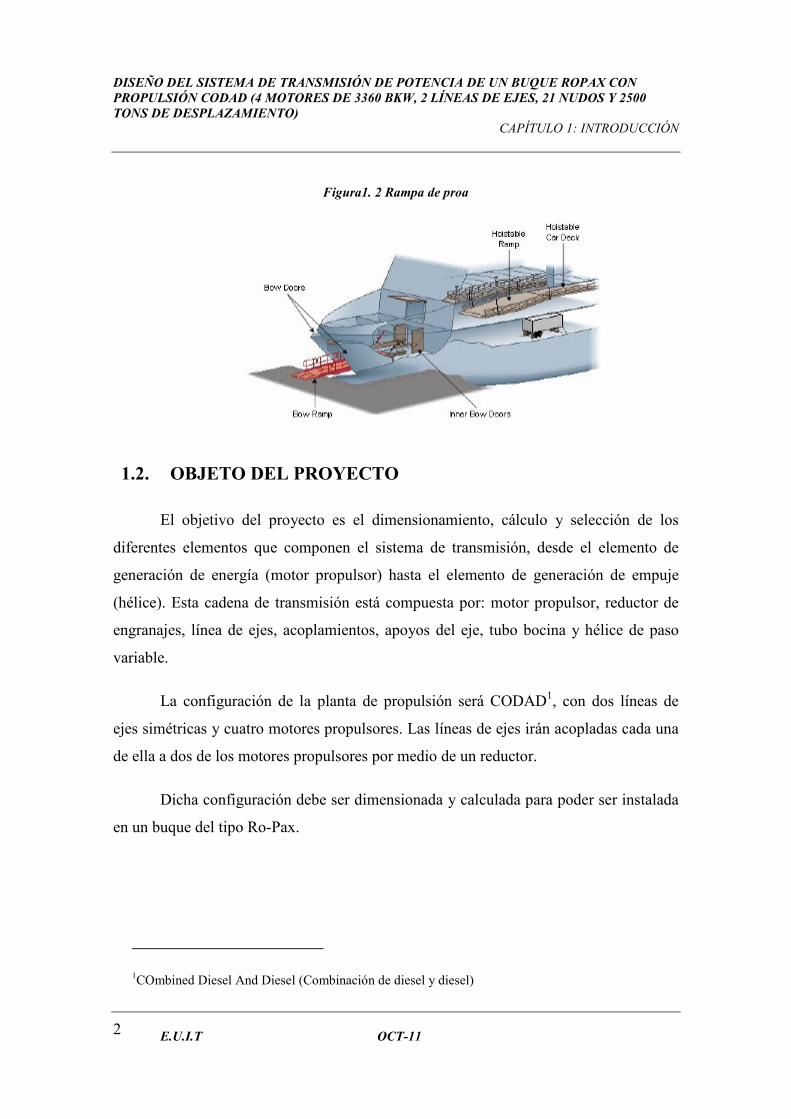
A continuación podemos ver las ilustraciones de buques Ro-Pax con rampas a
popa y a proa.
Figura1. 1 Rampa de popa
DISEÑO DEL SISTEMA DE TRANSMISIÓN DE POTENCIA DE UN BUQUE ROPAX CON PROPULSIÓN CODAD (4 MOTORES DE 3360 BKW, 2 LÍNEAS DE EJES, 21 NUDOS Y 2500 TONS DE DESPLAZAMIENTO)
CAPÍTULO 1: INTRODUCCIÓN
E.U.I.T OCT-11 2
Figura1. 2 Rampa de proa
1.2. OBJETO DEL PROYECTO
El objetivo del proyecto es el dimensionamiento, cálculo y selección de los
diferentes elementos que componen el sistema de transmisión, desde el elemento de
generación de energía (motor propulsor) hasta el elemento de generación de empuje
(hélice). Esta cadena de transmisión está compuesta por: motor propulsor, reductor de
engranajes, línea de ejes, acoplamientos, apoyos del eje, tubo bocina y hélice de paso
variable.
La configuración de la planta de propulsión será CODAD1, con dos líneas de
ejes simétricas y cuatro motores propulsores. Las líneas de ejes irán acopladas cada una
de ella a dos de los motores propulsores por medio de un reductor.
Dicha configuración debe ser dimensionada y calculada para poder ser instalada
en un buque del tipo Ro-Pax.
1COmbined Diesel And Diesel (Combinación de diesel y diesel)
DISEÑO DEL SISTEMA DE TRANSMISIÓN DE POTENCIA DE UN BUQUE ROPAX CON PROPULSIÓN CODAD (4 MOTORES DE 3360 BKW, 2 LÍNEAS DE EJES, 21 NUDOS Y 2500 TONS DE DESPLAZAMIENTO)
CAPÍTULO 1: INTRODUCCIÓN
E.U.I.T OCT-11 3
1.3. REFERENCIAS TÉCNICAS DE LA PLATAFORMA
El buque está diseñado para operar en condiciones de vientos de fuerte
intensidad, elevados estados de la mar y en puertos con accesos extremadamente
complicados. En estas condiciones, es requerimiento habitual diseñar los sistemas para
temperaturas ambientales de hasta -20 ºC. Su capacidad de carga admite además de
pasajeros, coches, traileres, MAFI traileres, caravanas y mercancías peligrosas en dos
cubiertas de garaje, una de ellas móvil del tipo car-deck. Los accesos de vehículos y
pasajeros al buque se realizan mediante dos rampas situadas en popa y una rampa
situada en el costado de estribor. La planta propulsora está compuesta por cuatro
motores diesel MAN B&W 7L 32/40 acoplados por parejas a reductores de doble
entrada que accionan líneas de ejes con hélices de paso variable. La generación de
energía a bordo la realizan cuatro grupos generadores accionados por motores diesel y
un generador de emergencia.
Dispone de dos hélices de maniobra en proa accionadas por motores eléctricos;
tanques de compensación de escora con capacidad suficiente para contrarrestar la acción
de dos traileres moviéndose simultáneamente a lo largo de una misma banda y de una
pareja de aletas estabilizadoras del tipo replegable, que permiten una reducción de hasta
un 90 % del movimiento de balance del buque.
La cámara de máquinas está totalmente automatizada, cumpliendo íntegramente
con los requerimientos de la Sociedad de Clasificación para cámara de máquinas
desatendida, pudiéndose controlar todos los parámetros de funcionamiento desde la
consola de control del puente de gobierno.
DISEÑO DEL SISTEMA DE TRANSMISIÓN DE POTENCIA DE UN BUQUE ROPAX CON PROPULSIÓN CODAD (4 MOTORES DE 3360 BKW, 2 LÍNEAS DE EJES, 21 NUDOS Y 2500 TONS DE DESPLAZAMIENTO)
CAPÍTULO 1: INTRODUCCIÓN
E.U.I.T OCT-11 4
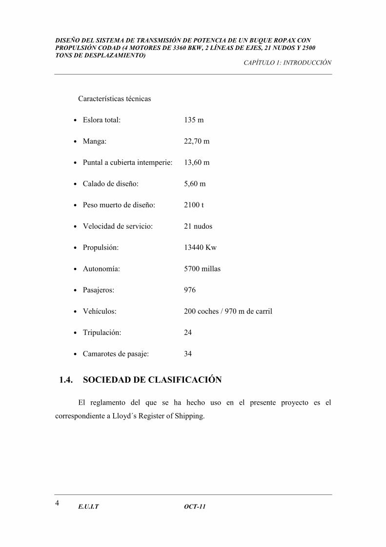
Características técnicas
• Eslora total: 135 m
• Manga: 22,70 m
• Puntal a cubierta intemperie: 13,60 m
• Calado de diseño: 5,60 m
• Peso muerto de diseño: 2100 t
• Velocidad de servicio: 21 nudos
• Propulsión: 13440 Kw
• Autonomía: 5700 millas
• Pasajeros: 976
• Vehículos: 200 coches / 970 m de carril
• Tripulación: 24
• Camarotes de pasaje: 34
1.4. SOCIEDAD DE CLASIFICACIÓN
El reglamento del que se ha hecho uso en el presente proyecto es el
correspondiente a Lloyd´s Register of Shipping.
DISEÑO DEL SISTEMA DE TRANSMISIÓN DE POTENCIA DE UN BUQUE ROPAX CON PROPULSIÓN CODAD (4 MOTORES DE 3360 BKW, 2 LÍNEAS DE EJES, 21 NUDOS Y 2500 TONS DE DESPLAZAMIENTO)
CAPÍTULO 2: DATOS FUNCIONALES DE DISEÑO
E.U.I.T OCT-11 5
CAPÍTULO 2. DATOS FUNCIONALES DE DISEÑO
2.1. REFERENCIAS DE EQUIPOS Y ELEMENTOS
MECÁNICOS
2.1.1. Motores propulsores
• Fabricante: IZAR-MOTORES
• Modelo: 7 L 32/40
• Ciclos: 4 Tiempos
• Combustible: Diesel
• MCR2 (kW): 3360
• Número de pistones: 7 en línea
• Carrera del pistón: 400 mm
• Diámetro del pistón: 320 mm.
• Velocidad de giro del motor: 750 rpm
2 Potencia máxima continua
DISEÑO DEL SISTEMA DE TRANSMISIÓN DE POTENCIA DE UN BUQUE ROPAX CON PROPULSIÓN CODAD (4 MOTORES DE 3360 BKW, 2 LÍNEAS DE EJES, 21 NUDOS Y 2500 TONS DE DESPLAZAMIENTO)
CAPÍTULO 2: DATOS FUNCIONALES DE DISEÑO
E.U.I.T OCT-11 6
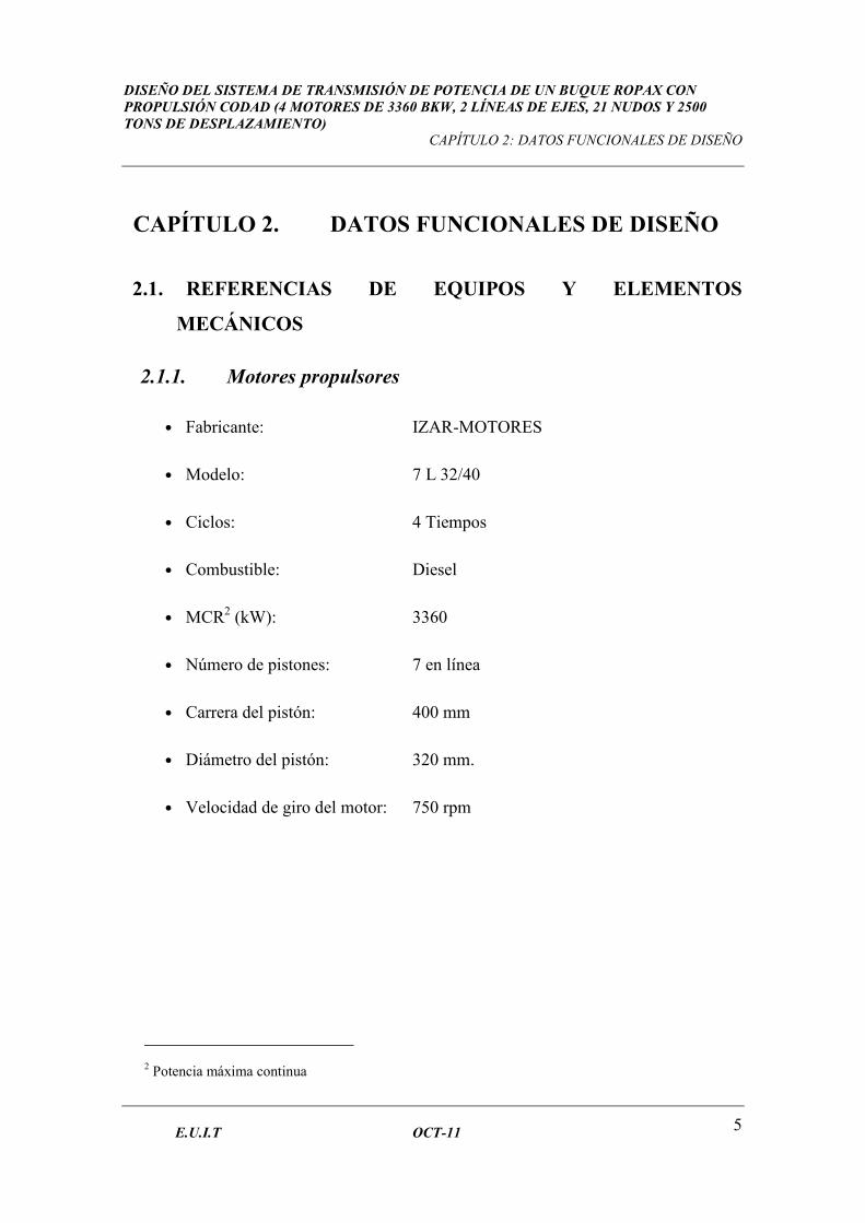
Figura 2. 1 Dimensiones del motor
Catálogo MAN
Tabla: 2.1 Dimensiones principales del motor
Dimensiones principales
Longitud L Ancho W Altura H Peso sin el volante
6470 mm 2630 mm 4010 mm 42 t
Catálogo MAN
El rango de operación del motor para hélices de paso variable se muestra a
continuación.

DISEÑO DEL SISTEMA DE TRANSMISIÓN DE POTENCIA DE UN BUQUE ROPAX CON PROPULSIÓN CODAD (4 MOTORES DE 3360 BKW, 2 LÍNEAS DE EJES, 21 NUDOS Y 2500 TONS DE DESPLAZAMIENTO)
CAPÍTULO 2: DATOS FUNCIONALES DE DISEÑO
E.U.I.T OCT-11 7
Figura 2. 2 Curva del motor para hélice paso variable
Catálogo MAN
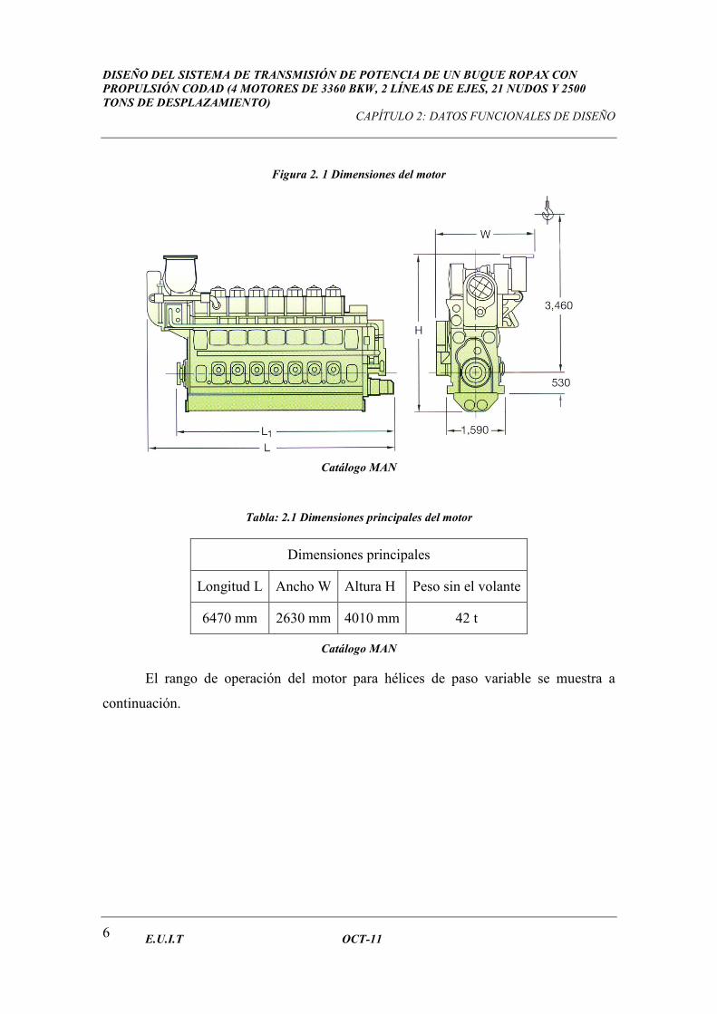
El numero totales de motores serán cuatro, con una configuración de dos
motores por reductor y eje. La distancia mínima de montaje para motores en paralelo, es
la que se muestra en la figura 2.3
DISEÑO DEL SISTEMA DE TRANSMISIÓN DE POTENCIA DE UN BUQUE ROPAX CON PROPULSIÓN CODAD (4 MOTORES DE 3360 BKW, 2 LÍNEAS DE EJES, 21 NUDOS Y 2500 TONS DE DESPLAZAMIENTO)
CAPÍTULO 2: DATOS FUNCIONALES DE DISEÑO
E.U.I.T OCT-11 8
Figura 2. 3 Dimensiones mín. entre motores paralelos y mamparos adyacentes
Catálogo MAN
2.1.2. Reductor
La reductora pertenece a la casa Reintjes modelo DLG 5551 K41 con una
relación de reducción de 5:1
Está compuesta por los siguientes elementos:
• Embragues: El accionamiento de los mismos es hidráulico. Llevan incorporado
sus propios sistemas de refrigeración y elementos para su control y seguridad.
• Dos entradas de ejes. La distancia mínima entre las entradas es de 2500 mm.
DISEÑO DEL SISTEMA DE TRANSMISIÓN DE POTENCIA DE UN BUQUE ROPAX CON PROPULSIÓN CODAD (4 MOTORES DE 3360 BKW, 2 LÍNEAS DE EJES, 21 NUDOS Y 2500 TONS DE DESPLAZAMIENTO)
CAPÍTULO 2: DATOS FUNCIONALES DE DISEÑO
E.U.I.T OCT-11 9
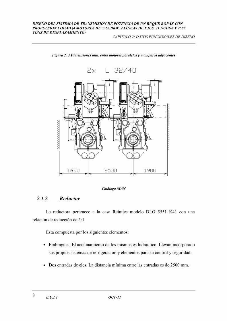
• Una salida de eje PTO3 para conducir el alternador principal.
• Engranajes endurecidos y de alta resistencia.
• Un cojinete de empuje incorporado para soportar los máximos empujes de la
hélice hacia proa y hacia popa.
• Dos bombas de aceite.
• Dos válvulas de control
• Dos filtros de aceite.
• Dos cambiadores de calor.
Figura 2. 4 Caja reductora
Reintjes reductores
3 Power TakeOff (Toma de fuerza)
DISEÑO DEL SISTEMA DE TRANSMISIÓN DE POTENCIA DE UN BUQUE ROPAX CON PROPULSIÓN CODAD (4 MOTORES DE 3360 BKW, 2 LÍNEAS DE EJES, 21 NUDOS Y 2500 TONS DE DESPLAZAMIENTO)
CAPÍTULO 2: DATOS FUNCIONALES DE DISEÑO
E.U.I.T OCT-11 10
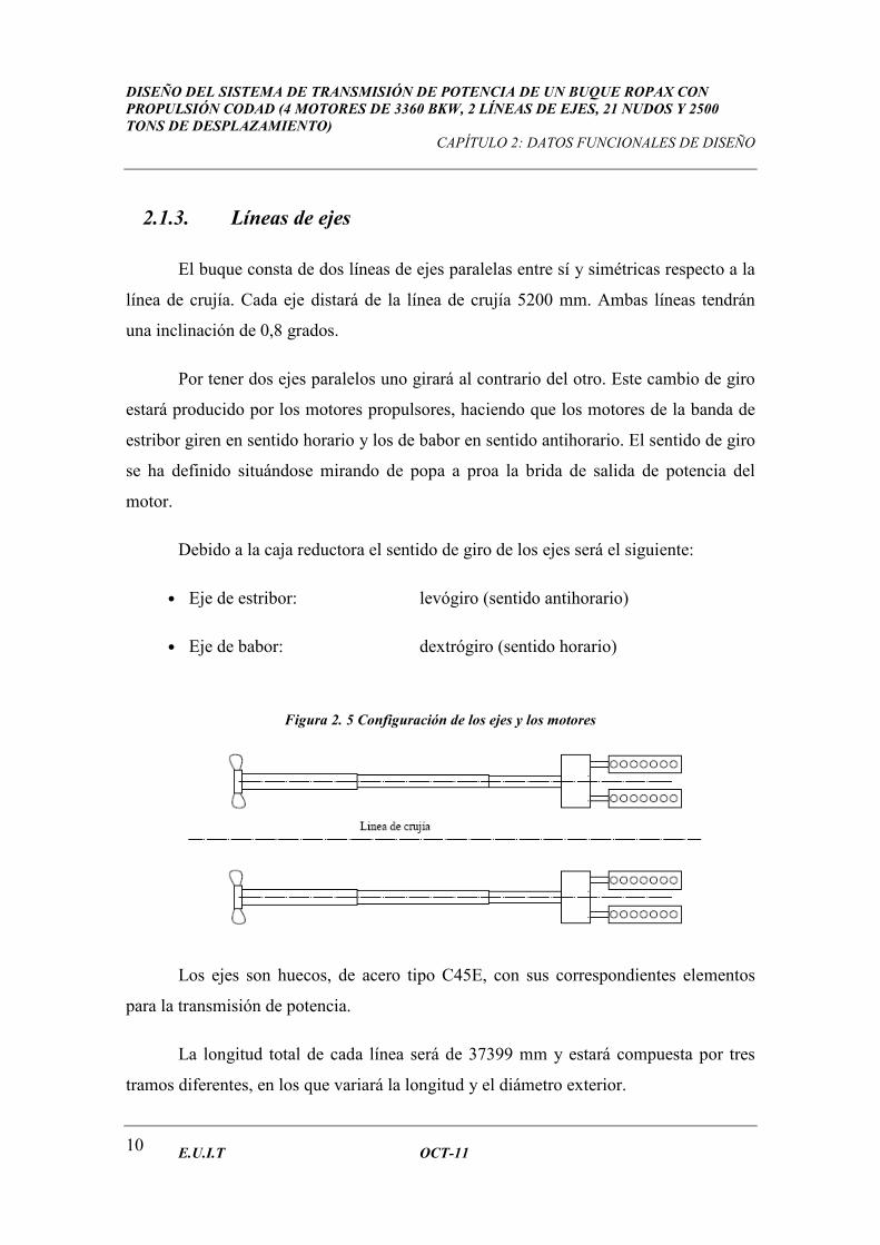
2.1.3. Líneas de ejes
El buque consta de dos líneas de ejes paralelas entre sí y simétricas respecto a la
línea de crujía. Cada eje distará de la línea de crujía 5200 mm. Ambas líneas tendrán
una inclinación de 0,8 grados.
Por tener dos ejes paralelos uno girará al contrario del otro. Este cambio de giro
estará producido por los motores propulsores, haciendo que los motores de la banda de
estribor giren en sentido horario y los de babor en sentido antihorario. El sentido de giro
se ha definido situándose mirando de popa a proa la brida de salida de potencia del
motor.
Debido a la caja reductora el sentido de giro de los ejes será el siguiente:
• Eje de estribor: levógiro (sentido antihorario)
• Eje de babor: dextrógiro (sentido horario)
Figura 2. 5 Configuración de los ejes y los motores
Los ejes son huecos, de acero tipo C45E, con sus correspondientes elementos
para la transmisión de potencia.
La longitud total de cada línea será de 37399 mm y estará compuesta por tres
tramos diferentes, en los que variará la longitud y el diámetro exterior.
DISEÑO DEL SISTEMA DE TRANSMISIÓN DE POTENCIA DE UN BUQUE ROPAX CON PROPULSIÓN CODAD (4 MOTORES DE 3360 BKW, 2 LÍNEAS DE EJES, 21 NUDOS Y 2500 TONS DE DESPLAZAMIENTO)
CAPÍTULO 2: DATOS FUNCIONALES DE DISEÑO
E.U.I.T OCT-11 11
El diámetro interior será el hueco por donde se canalizarán los tubos hidráulicos
para operar la hélice de paso variable. Será el mismo en los tres tramos.
Todas las longitudes y diámetros cumplirán con la normativa de la Sociedad de
Clasificación.
2.1.4. Acoplamientos
Se usarán acoplamientos de interferencia por presión hidráulica del tipo eje-eje,
eje-máquina de la casa SKF.
2.1.5. Cojinetes de apoyo de los ejes
Los cojinetes de apoyo, tanto los del tubo de bocina como los intermedios, serán
de metal blanco del fabricante Cedervall & Söner.
2.1.6. Sellos del tubo de bocina
La misión de los sellos de bocina es evitar que el agua del mar pueda entrar en el
buque, y a su vez evitar que el aceite de refrigeración de los cojinetes del tubo de bocina
sea vertido al mar. Serán dos y del fabricante Cedervall & Söner.
2.1.7. Pasamamparo estanco del eje
La misión del pasamamparo estanco es evitar que un compartimento pierda su
estanqueidad por la abertura practicada en el mamparo por donde pasa el eje.
2.1.8. Tubo de Bocina
El eje de cola ha de pasar a través del casco del buque en la zona de obra viva,
paso que necesariamente debe quedar en forma estanca al agua de mar. Esta
estanqueidad se consigue por medio de la bocina que cumple una doble misión: servir
de soporte al eje y asegurar la citada estanqueidad por medio de dos sellos hidráulicos.
DISEÑO DEL SISTEMA DE TRANSMISIÓN DE POTENCIA DE UN BUQUE ROPAX CON PROPULSIÓN CODAD (4 MOTORES DE 3360 BKW, 2 LÍNEAS DE EJES, 21 NUDOS Y 2500 TONS DE DESPLAZAMIENTO)
CAPÍTULO 2: DATOS FUNCIONALES DE DISEÑO
E.U.I.T OCT-11 12
Estará formado básicamente de un tubo, que servirá de soporte y protegerá el
tramo del eje que queda fuera del casco del buque. El tubo dispone de un sello
hidráulico en cada uno de sus extremos, cuya misión será la de impedir que pueda entrar
el agua salada dentro del buque y evitar que salga el aceite en el que está sumergido el
tramo de eje. Este aceite proviene de un tanque de compensación que le proporciona,
además, una presión superior que la del exterior del tubo de bocina, evitando en todo
momento la entrada de agua salada.
2.1.9. Hélice
Nuestra hélice será de paso variable (KAMEWA 102 XF5/4) y sus principales
características son:
• Peso: 7100 Kg
• Número de palas: 4
• Diámetro: 4300 mm
• Velocidad: 150 rpm
• Material: CuNiAl
2.1.10. Cálculo curva de potencia
Una ecuación aproximada de la curva de demanda de potencia absorbida por el
consumidor, en función de su velocidad, es:
33 nKnFPot ×=×=
Donde:
• Pot: Potencia absorbida por el consumidor y medida en DkW.
DISEÑO DEL SISTEMA DE TRANSMISIÓN DE POTENCIA DE UN BUQUE ROPAX CON PROPULSIÓN CODAD (4 MOTORES DE 3360 BKW, 2 LÍNEAS DE EJES, 21 NUDOS Y 2500 TONS DE DESPLAZAMIENTO)
CAPÍTULO 2: DATOS FUNCIONALES DE DISEÑO
E.U.I.T OCT-11 13
• n: Revoluciones de giro del consumidor.
• K: Es una constante.
Los datos de diseño para la determinación de la curva de potencia son:
• Potencia máxima entregada al eje.
• Revoluciones a las que gira la hélice.
El diseño constará de dos ejes, cada uno de ellos acoplado a dos motores
mediante una reductora. Con dicha configuración (motores más reductor), se dispondrá
de una potencia en la entrada del reductor de 6720 BkW4, a 750 rpm y en la salida
obtendremos 6518,4 DkW5 a 150 rpm, teniendo en cuenta que hay una pérdida del 3%
por rozamiento en el reductor.
El valor de K puede ser constante o variable en función de si la hélice que se
use, sea de paso fijo o controlable. En este caso la hélice es de paso variable, lo cual
presenta la ventaja de poder modificar el ángulo de ataque de las palas y así variar el
paso de la misma. Por lo tanto K será variable, logrando así optimizar el consumo de
potencia y el de combustible en función de las condiciones operativas del buque.
El valor de K se obtiene despejando en la siguiente fórmula:
33 nKnFPot ×=×= (2.1)
( ) 333
1093,1150
4,6518
n
DkWPotK −
×===
• Pot = 6518,4 DkW
4 Brake Kilowatio (Potencia en el freno) 5Delivered Kilowatio (Potencia entregada)
DISEÑO DEL SISTEMA DE TRANSMISIÓN DE POTENCIA DE UN BUQUE ROPAX CON PROPULSIÓN CODAD (4 MOTORES DE 3360 BKW, 2 LÍNEAS DE EJES, 21 NUDOS Y 2500 TONS DE DESPLAZAMIENTO)
CAPÍTULO 2: DATOS FUNCIONALES DE DISEÑO
E.U.I.T OCT-11 14
• n = 150 rpm
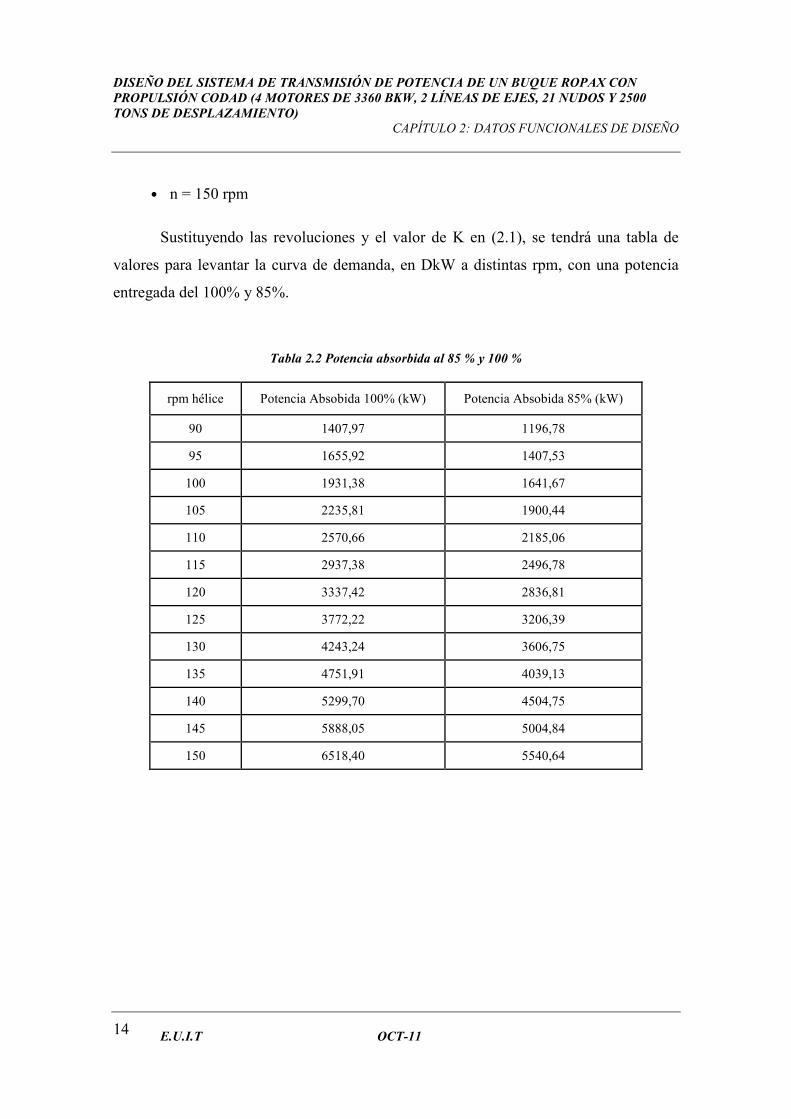
Sustituyendo las revoluciones y el valor de K en (2.1), se tendrá una tabla de
valores para levantar la curva de demanda, en DkW a distintas rpm, con una potencia
entregada del 100% y 85%.
Tabla 2.2 Potencia absorbida al 85 % y 100 %
rpm hélice Potencia Absobida 100% (kW) Potencia Absobida 85% (kW)
90 1407,97 1196,78
95 1655,92 1407,53
100 1931,38 1641,67
105 2235,81 1900,44
110 2570,66 2185,06
115 2937,38 2496,78
120 3337,42 2836,81
125 3772,22 3206,39
130 4243,24 3606,75
135 4751,91 4039,13
140 5299,70 4504,75
145 5888,05 5004,84
150 6518,40 5540,64
DISEÑO DEL SISTEMA DE TRANSMISIÓN DE POTENCIA DE UN BUQUE ROPAX CON PROPULSIÓN CODAD (4 MOTORES DE 3360 BKW, 2 LÍNEAS DE EJES, 21 NUDOS Y 2500 TONS DE DESPLAZAMIENTO)
CAPÍTULO 2: DATOS FUNCIONALES DE DISEÑO
E.U.I.T OCT-11 15
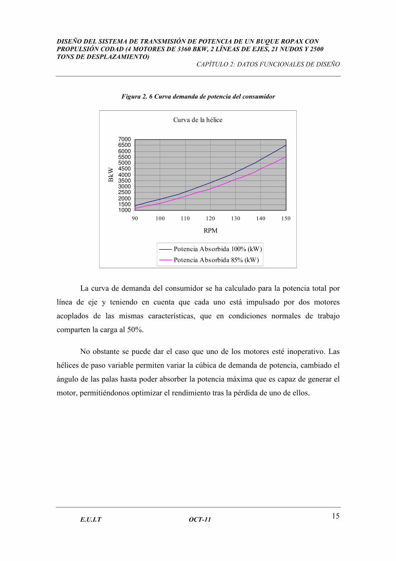
Figura 2. 6 Curva demanda de potencia del consumidor
Curva de la hélice
1000
1500
2000
2500
3000
3500
4000
4500
5000
5500
6000
6500
7000
90 100 110 120 130 140 150
RPM
BkW
Potencia Absorbida 100% (kW)
Potencia Absorbida 85% (kW)
La curva de demanda del consumidor se ha calculado para la potencia total por
línea de eje y teniendo en cuenta que cada uno está impulsado por dos motores
acoplados de las mismas características, que en condiciones normales de trabajo
comparten la carga al 50%.
No obstante se puede dar el caso que uno de los motores esté inoperativo. Las
hélices de paso variable permiten variar la cúbica de demanda de potencia, cambiado el
ángulo de las palas hasta poder absorber la potencia máxima que es capaz de generar el
motor, permitiéndonos optimizar el rendimiento tras la pérdida de uno de ellos.

DISEÑO DEL SISTEMA DE TRANSMISIÓN DE POTENCIA DE UN BUQUE ROPAX CON PROPULSIÓN CODAD (4 MOTORES DE 3360 BKW, 2 LÍNEAS DE EJES, 21 NUDOS Y 2500 TONS DE DESPLAZAMIENTO)
CAPÍTULO 3: DIÁMETRO DEL EJE POR CÁLCULO DIRECTO
E.U.I.T OCT-11 17
CAPÍTULO 3. DIÁMETRO DEL EJE POR CÁLCULO
DIRECTO
3.1. CÁLCULO MOMENTO TORSOR
Sabiendo que el eje estará sometido a torsión, flexión y fuerza axial, los cálculos
se realizarán básicamente para el esfuerzo a torsión, ya que es el más restrictivo. Los
demás esfuerzos se tendrán en cuenta y estarán controlados.
Como dato de partida, se conoce la potencia que se entrega al eje, las
revoluciones a las que girará y el diámetro interior. Este diámetro interior viene
impuesto por la hélice para poder alojar los circuitos hidráulicos que accionan sus palas.
La potencia entregada a la hélice (DkW) será la suma de la potencia de dos
motores menos las pérdidas por rozamiento del reductor 3%.
• DkW= 3360×2×0,97= 6518,40 kW
• Rpm= 150
• Diámetro interior (d)= 110 mm.
• Tipo de acero del eje= C45E
Teniendo todo esto en cuenta, el momento torsor de diseño del eje viene dado
por:
RPM
kW55,9Mt
×=
.mkN415150
4,651855,9Mt ×=
×=
DISEÑO DEL SISTEMA DE TRANSMISIÓN DE POTENCIA DE UN BUQUE ROPAX CON PROPULSIÓN CODAD (4 MOTORES DE 3360 BKW, 2 LÍNEAS DE EJES, 21 NUDOS Y 2500 TONS DE DESPLAZAMIENTO)
CAPÍTULO 3: DIÁMETRO DEL EJE POR CÁLCULO DIRECTO
E.U.I.T OCT-11 18
3.2. TENSIÓN CORTANTE MÁXIMA
La tensión cortante (τcort) viene dada aproximadamente por:
3elast
cortσ
=τ (3.1)
Como el tipo de acero del eje tiene un límite elástico (σelast) de 330 N/mm2,
despejando en (3.1) se obtiene:
2mmN531903
330/,max ==τ
NOTA: Habrá que tener en cuenta que si se toma este valor de tensión cortante
no se le estará aplicando ningún coeficiente de seguridad.
3.3. DIÁMETRO EXTERIOR DEL EJE
El diámetro exterior mínimo (D) del eje se calculará despejándolo de la fórmula:
( )44cortdD
DMt16
−×π
××=τ (3.2)
Para τcort= 190,53 N/mm2 , d = 110 mm y Mt = 415 kN × m se obtiene que: D=
227,26 mm.
3.4. REGLA DEL 30% (σσσσELAST) Ó 18% (σσσσMÁX.)
A falta de requerimiento específico, una forma habitual de calcular las tensiones
del eje es restringir el límite elástico (σelast) al 30% o límite máximo de rotura (σmáx.) al
18%. Se usará el menor de los resultados ya que es el más restrictivo como valor de la
tensión combinada (σcomb).
DISEÑO DEL SISTEMA DE TRANSMISIÓN DE POTENCIA DE UN BUQUE ROPAX CON PROPULSIÓN CODAD (4 MOTORES DE 3360 BKW, 2 LÍNEAS DE EJES, 21 NUDOS Y 2500 TONS DE DESPLAZAMIENTO)
CAPÍTULO 3: DIÁMETRO DEL EJE POR CÁLCULO DIRECTO
E.U.I.T OCT-11 19
30% de 330 N/mm2 = 99 N/mm2
18% de 600 N/ mm2 = 108 N/ mm2
El esfuerzo axial (σaxial) se hallará despejándolo de la fórmula:
tetancor2
axial2
comb 3 τ×+σ=σ ⇒ cort2
comb2
axial 3 τ×−σ=σ
Para σcombinada= 99 N/mm2 y restringiendo la tensión cortante a 55 N/mm2, se
obtiene:
222axial mm/N94,2655399 =×−=σ
Al restringir la tensión cortante se hace necesario recalcular el diámetro exterior
del eje. Se ha obtenido a partir de la fórmula (3.2) un valor de D = 338,72 mm.
3.5. MOMENTO FLECTOR
La resistencia de materiales nos dice que:
( )D32
dDM
44axial
f×
−×π×σ=
Sustituyendo los datos obtenidos en la fórmula se obtiene que:
( )mN03,101656
72,33832
11072,33894,26M
44
f ×=×
−×π×=
3.6. PESO DEL EJE POR METRO LINEAL
El peso del eje por metro lineal viene dado por:
gAm
peso××ρ=
DISEÑO DEL SISTEMA DE TRANSMISIÓN DE POTENCIA DE UN BUQUE ROPAX CON PROPULSIÓN CODAD (4 MOTORES DE 3360 BKW, 2 LÍNEAS DE EJES, 21 NUDOS Y 2500 TONS DE DESPLAZAMIENTO)
CAPÍTULO 3: DIÁMETRO DEL EJE POR CÁLCULO DIRECTO
E.U.I.T OCT-11 20
Donde:
• ρ = densidad acero 7850 Kg/m3
• A = área de la sección del eje mm2
• g = gravedad 9,81m/s2
El área de una sección transversal del eje será:
4
dDA
22 −×π=
222
mm39,806064
11072,338A =
−×π=
Con lo que se obtiene:
m/N38,620781,91039,806067850peso 6 =×××= −
3.7. DISTANCIA ENTRE APOYOS DEL EJE
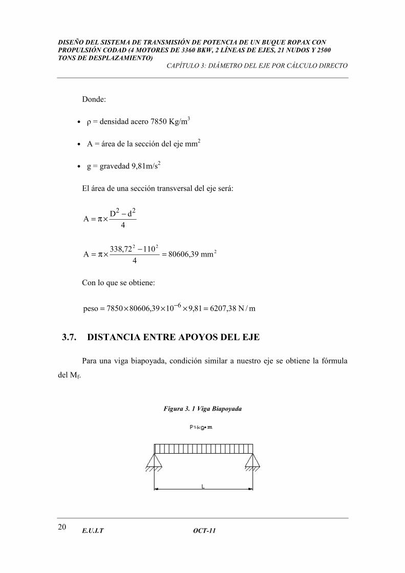
Para una viga biapoyada, condición similar a nuestro eje se obtiene la fórmula
del Mf.
Figura 3. 1 Viga Biapoyada
DISEÑO DEL SISTEMA DE TRANSMISIÓN DE POTENCIA DE UN BUQUE ROPAX CON PROPULSIÓN CODAD (4 MOTORES DE 3360 BKW, 2 LÍNEAS DE EJES, 21 NUDOS Y 2500 TONS DE DESPLAZAMIENTO)
CAPÍTULO 3: DIÁMETRO DEL EJE POR CÁLCULO DIRECTO
E.U.I.T OCT-11 21
Despejando la longitud (l):
peso
8Mfl
8
lpesoM
2
f×
=⇒×
=
Y usando los datos obtenidos por cálculo directo:
• Tensión combinada máxima = 99 N/mm2
• Tensión cortante máxima = 55 N/mm2
• Tensión axial máxima = 26,94 N/mm2
• Diámetro exterior del eje = 338,72 mm
• Diámetro interior del eje = 110 mm
Se tiene una distancia máxima entre apoyos del eje de:
.m45,1138,6207
803,101656l =
×=

DISEÑO DEL SISTEMA DE TRANSMISIÓN DE POTENCIA DE UN BUQUE ROPAX CON PROPULSIÓN CODAD (4 MOTORES DE 3360 BKW, 2 LÍNEAS DE EJES, 21 NUDOS Y 2500 TONS DE DESPLAZAMIENTO)
CAPÍTULO 4: DIMENSIONAMIENTO DE LA LINEA DE EJE POR LA LLOYD`S NAVAL
E.U.I.T OCT-11 23
CAPÍTULO 4. DIMENSIONAMIENTO DE LA LÍNEA
DE EJES POR LA LLOYD’S REGISTER
4.1. DATOS DE PARTIDA
En este capítulo se calculará el eje según las normas de la Sociedad de
Clasificación.
Los datos de partida y material del eje son:
• DkW= 3360×2×0,97= 6518,40
• Rpm= 150
• Diámetro interior (d)= 110 mm
• Tipo de acero del eje= C45E
La Sociedad de Clasificación diferencia tres diámetros exteriores según la
posición de los tramos:
• Tramo de eje de cola: es el tramo más próximo al propulsor.
• Tramo de eje intermedio: será continuación del eje de cola hasta sobrepasar
1500 milímetros del sello de proa del tubo de bocina.
• Tramo de eje de proa: será continuación del tramo intermedio hasta la brida de
acoplamiento del reductor.
Para evitar puntos de concentraciones de esfuerzos cortantes, la transición de los
distintos diámetros de los ejes se hará por una reducción progresiva del diámetro con
una inclinación de diez grados.
DISEÑO DEL SISTEMA DE TRANSMISIÓN DE POTENCIA DE UN BUQUE ROPAX CON PROPULSIÓN CODAD (4 MOTORES DE 3360 BKW, 2 LÍNEAS DE EJES, 21 NUDOS Y 2500 TONS DE DESPLAZAMIENTO)
CAPÍTULO 4: DIMENSIONAMIENTO DE LA LINEA DE EJE POR LA LLOYD`S NAVAL
E.U.I.T OCT-11 24
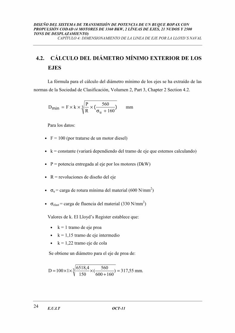
4.2. CÁLCULO DEL DIÁMETRO MÍNIMO EXTERIOR DE LOS
EJES
La fórmula para el cálculo del diámetro mínimo de los ejes se ha extraído de las
normas de la Sociedad de Clasificación, Volumen 2, Part 3, Chapter 2 Section 4.2.
mm160
560
R
PkFD 3
u)(min
+σ×××=
Para los datos:
• F = 100 (por tratarse de un motor diesel)
• k = constante (variará dependiendo del tramo de eje que estemos calculando)
• P = potencia entregada al eje por los motores (DkW)
• R = revoluciones de diseño del eje
• σu = carga de rotura mínima del material (600 N/mm2)
• σelast = carga de fluencia del material (330 N/mm2)
Valores de k. El Lloyd’s Register establece que:
• k = 1 tramo de eje proa
• k = 1,15 tramo de eje intermedio
• k = 1,22 tramo eje de cola
Se obtiene un diámetro para el eje de proa de:
.mm55,317)160600
560(
150
4,65181100D 3 =
+×××=
DISEÑO DEL SISTEMA DE TRANSMISIÓN DE POTENCIA DE UN BUQUE ROPAX CON PROPULSIÓN CODAD (4 MOTORES DE 3360 BKW, 2 LÍNEAS DE EJES, 21 NUDOS Y 2500 TONS DE DESPLAZAMIENTO)
CAPÍTULO 4: DIMENSIONAMIENTO DE LA LINEA DE EJE POR LA LLOYD`S NAVAL
E.U.I.T OCT-11 25
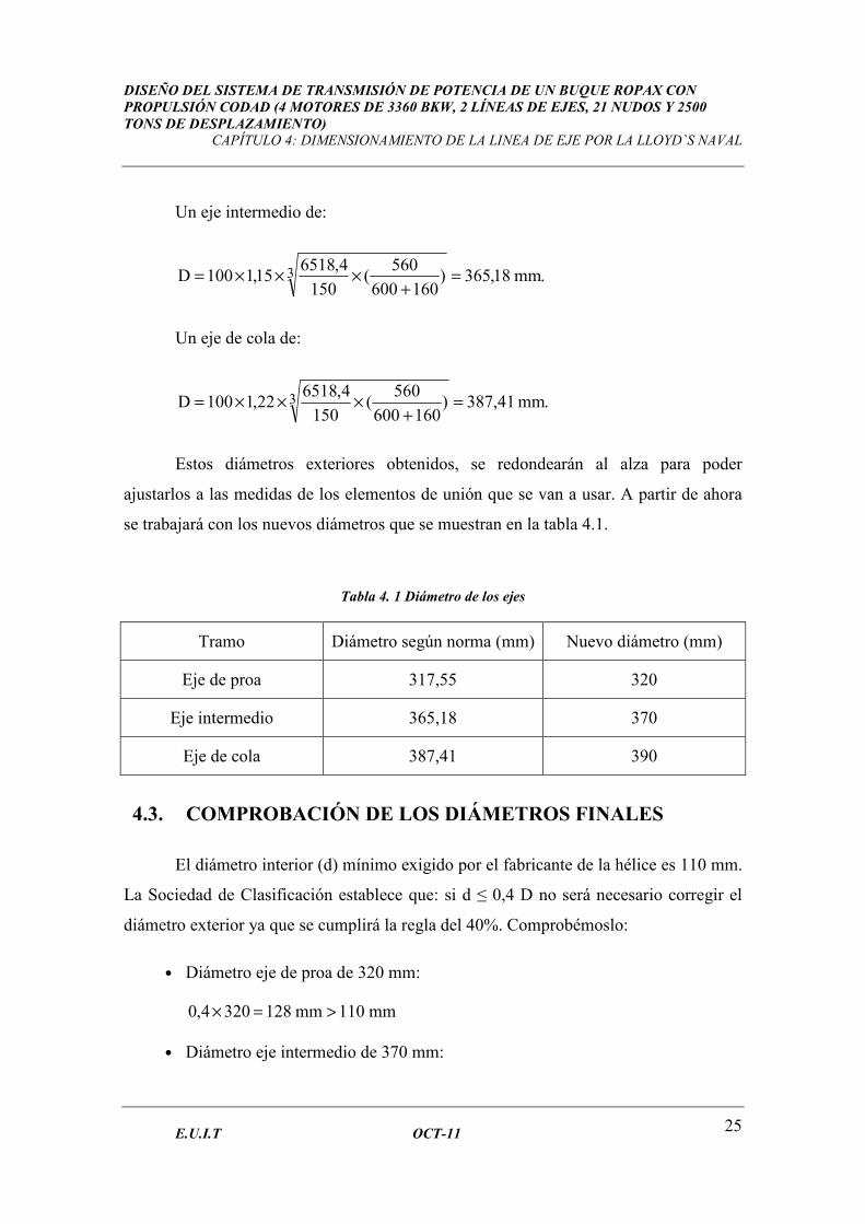
Un eje intermedio de:
.mm18,365)160600
560(
150
4,651815,1100D 3 =
+×××=
Un eje de cola de:
.mm41,387)160600
560(
150
4,651822,1100D 3 =
+×××=
Estos diámetros exteriores obtenidos, se redondearán al alza para poder
ajustarlos a las medidas de los elementos de unión que se van a usar. A partir de ahora
se trabajará con los nuevos diámetros que se muestran en la tabla 4.1.
Tabla 4. 1 Diámetro de los ejes
Tramo Diámetro según norma (mm) Nuevo diámetro (mm)
Eje de proa 317,55 320
Eje intermedio 365,18 370
Eje de cola 387,41 390
4.3. COMPROBACIÓN DE LOS DIÁMETROS FINALES
El diámetro interior (d) mínimo exigido por el fabricante de la hélice es 110 mm.
La Sociedad de Clasificación establece que: si d ≤ 0,4 D no será necesario corregir el
diámetro exterior ya que se cumplirá la regla del 40%. Comprobémoslo:
• Diámetro eje de proa de 320 mm:
mm110mm128 3204,0 >=×
• Diámetro eje intermedio de 370 mm:
DISEÑO DEL SISTEMA DE TRANSMISIÓN DE POTENCIA DE UN BUQUE ROPAX CON PROPULSIÓN CODAD (4 MOTORES DE 3360 BKW, 2 LÍNEAS DE EJES, 21 NUDOS Y 2500 TONS DE DESPLAZAMIENTO)
CAPÍTULO 4: DIMENSIONAMIENTO DE LA LINEA DE EJE POR LA LLOYD`S NAVAL
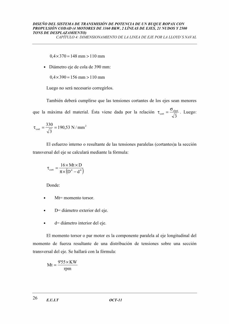
E.U.I.T OCT-11 26
mm110mm148 3704,0 >=×
• Diámetro eje de cola de 390 mm:
mm110mm156 3904,0 >=×
Luego no será necesario corregirlos.
También deberá cumplirse que las tensiones cortantes de los ejes sean menores
que la máxima del material. Ésta viene dada por la relación 3
elastcort
σ=τ . Luego:
2cort mm/N53,190
3
330==τ
El esfuerzo interno o resultante de las tensiones paralelas (cortantes)a la sección
transversal del eje se calculará mediante la fórmula:
( )44cortdD
DMt16
−×π
××=τ
Donde:
• Mt= momento torsor.
• D= diámetro exterior del eje.
• d= diámetro interior del eje.
El momento torsor o par motor es la componente paralela al eje longitudinal del
momento de fuerza resultante de una distribución de tensiones sobre una sección
transversal del eje. Se hallará con la fórmula:
rpm
KW55'9Mt
×=
DISEÑO DEL SISTEMA DE TRANSMISIÓN DE POTENCIA DE UN BUQUE ROPAX CON PROPULSIÓN CODAD (4 MOTORES DE 3360 BKW, 2 LÍNEAS DE EJES, 21 NUDOS Y 2500 TONS DE DESPLAZAMIENTO)
CAPÍTULO 4: DIMENSIONAMIENTO DE LA LINEA DE EJE POR LA LLOYD`S NAVAL
E.U.I.T OCT-11 27
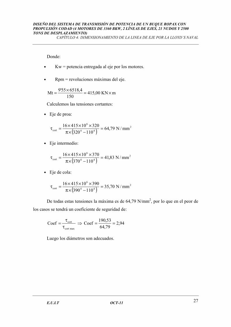
Donde:
• Kw = potencia entregada al eje por los motores.
• Rpm = revoluciones máximas del eje.
mKN00,415150
4,651855'9Mt ×=
×=
Calculemos las tensiones cortantes:
• Eje de proa:
( )2
44
6
cort mm/N79,64110320
3201041516=
−×π
×××=τ
• Eje intermedio:
( )2
44
6
cort mm/N83,41110370
3701041516=
−×π
×××=τ
• Eje de cola:
( )2
44
6
cort mm/N70,35110390
3901041516=
−×π
×××=τ
De todas estas tensiones la máxima es de 64,79 N/mm2, por lo que en el peor de
los casos se tendrá un coeficiente de seguridad de:
maxcort
cortCoefτ
τ= ⇒ 94,2
79,64
53,190Coef ==
Luego los diámetros son adecuados.

DISEÑO DEL SISTEMA DE TRANSMISIÓN DE POTENCIA DE UN BUQUE ROPAX CON PROPULSIÓN CODAD (4 MOTORES DE 3360 BKW, 2 LÍNEAS DE EJES, 21 NUDOS Y 2500 TONS DE DESPLAZAMIENTO)
CAPÍTULO 5: SEPARACIÓN MÁXIMA ENTRE APOYOS DE LOS EJES
E.U.I.T OCT-11 29
CAPÍTULO 5. SEPARACIÓN MÁXIMA ENTRE
APOYOS DE LOS EJES
5.1. SEPARACIÓN MÁXIMA ENTRE APOYOS
El objetivo fundamental es poner el menor número posible de soportes a lo largo
de la línea de eje, sin olvidar en ningún momento, la seguridad de la instalación ni las
normas de la Sociedad de Clasificación.
Se empezará calculando las distancias entre apoyos, usando los diámetros
exteriores obtenidos anteriormente, el diámetro interior de 110 mm y la longitud del eje
37399 mm (distancia comprendida entre la brida del reductor y la conexión con el
núcleo de la hélice).
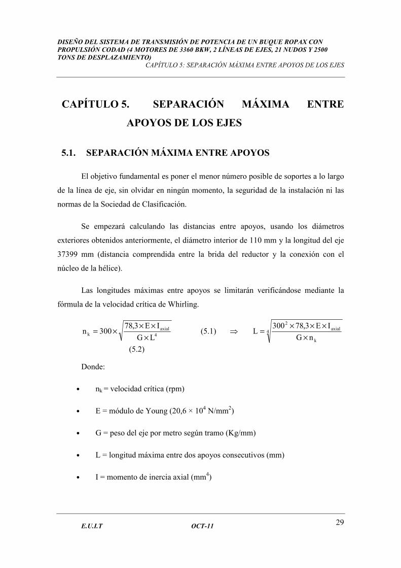
Las longitudes máximas entre apoyos se limitarán verificándose mediante la
fórmula de la velocidad crítica de Whirling.
4axial
kLG
IE3,78300n
×
×××= (5.1) ⇒ 4
k
axial2
nG
IE3,78300L
×
×××=
(5.2)
Donde:
• nk = velocidad crítica (rpm)
• E = módulo de Young (20,6 × 10⁴ N/mm2)
• G = peso del eje por metro según tramo (Kg/mm)
• L = longitud máxima entre dos apoyos consecutivos (mm)
• I = momento de inercia axial (mm4)
DISEÑO DEL SISTEMA DE TRANSMISIÓN DE POTENCIA DE UN BUQUE ROPAX CON PROPULSIÓN CODAD (4 MOTORES DE 3360 BKW, 2 LÍNEAS DE EJES, 21 NUDOS Y 2500 TONS DE DESPLAZAMIENTO)
CAPÍTULO 5: SEPARACIÓN MÁXIMA ENTRE APOYOS DE LOS EJES
E.U.I.T OCT-11 30
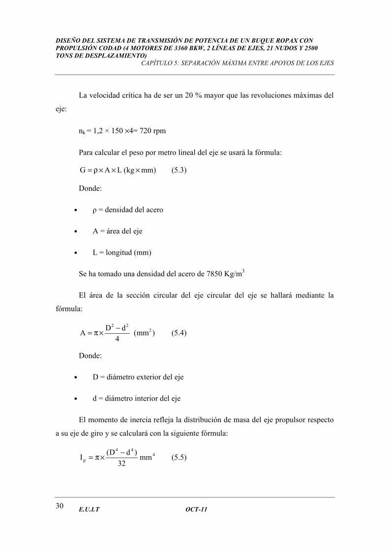
La velocidad crítica ha de ser un 20 % mayor que las revoluciones máximas del
eje:
nk = 1,2 × 150 ×4= 720 rpm
Para calcular el peso por metro lineal del eje se usará la fórmula:
)mmkg(LAG ×××ρ= (5.3)
Donde:
• ρ = densidad del acero
• A = área del eje
• L = longitud (mm)
Se ha tomado una densidad del acero de 7850 Kg/m3
El área de la sección circular del eje circular del eje se hallará mediante la
fórmula:
)mm(4
dDA 2
22−
×π= (5.4)
Donde:
• D = diámetro exterior del eje
• d = diámetro interior del eje
El momento de inercia refleja la distribución de masa del eje propulsor respecto
a su eje de giro y se calculará con la siguiente fórmula:
444
p mm32
)dD(I
−×π= (5.5)

DISEÑO DEL SISTEMA DE TRANSMISIÓN DE POTENCIA DE UN BUQUE ROPAX CON PROPULSIÓN CODAD (4 MOTORES DE 3360 BKW, 2 LÍNEAS DE EJES, 21 NUDOS Y 2500 TONS DE DESPLAZAMIENTO)
CAPÍTULO 5: SEPARACIÓN MÁXIMA ENTRE APOYOS DE LOS EJES
E.U.I.T OCT-11 31
5.1.1. Cálculo de la distancia máxima del eje de proa
222
mm45,709214
110320A =
−×π= ⇒ A= 0,070921 m2
( )mmkg56,0G)mkg(73,5561070921,07850G ×=⇒×=××=
4p
444
p m0010150633,0Imm,59101506331232
)110320(I =⇒=
−×π=
mm06,845372056,0
59,1015063312106,203,78300L 4
42=
×
××××=
5.1.2. Cálculo de la distancia máxima del eje intermedio
222
mm69,980174
110370A =
−×π= ⇒ A= 0,098018 m2
( )mmkg77,0G)mkg(44,7691098018,07850G ×=⇒×=××=
444
p mm00,182557949132
)110370(I =
−×π= ⇒ Ip = 0,0018255795 m
4
mm34,902872077,0
00,1825579491106,203,78300L 4
42=
×
××××=
5.1.3. Cálculo de la distancia máxima del eje de cola
222
mm74,1099554
110390A =
−×π= ⇒ A = 0,109956 m2
( )mmkg86,0G)mkg(15,8631109956,07850G ×=⇒×=××=
DISEÑO DEL SISTEMA DE TRANSMISIÓN DE POTENCIA DE UN BUQUE ROPAX CON PROPULSIÓN CODAD (4 MOTORES DE 3360 BKW, 2 LÍNEAS DE EJES, 21 NUDOS Y 2500 TONS DE DESPLAZAMIENTO)
CAPÍTULO 5: SEPARACIÓN MÁXIMA ENTRE APOYOS DE LOS EJES
E.U.I.T OCT-11 32
444
p mm52,225684162232
)110390(I =
−×π= ⇒ Ip = 0,0022568416 m
4
mm29,925072086,0
52,2256841622106,203,78300L 4
42=
×
××××=
5.2. SITUACIÓN DE LOS APOYOS
Una vez calculadas las distancias máximas de los apoyos, habrá que ver cuántos
y dónde se van a poner, teniendo en cuenta los requisitos siguientes:
• El primer apoyo será el inmediato al propulsor. Estará situado lo más
próximo posible a la hélice, para reducir al máximo el momento flector, debido
al gran peso de la misma.
• Todos los apoyos deben transmitir los esfuerzos a través de la estructura del
buque.
• El intervalo entre dos apoyos consecutivos no debe superar la distancia
máxima.
Para ubicar la situación de de los apoyos, se aprovecharán los elementos
resistentes de la estructura teniendo en cuenta que no superen las distancias máximas.
Una vez definida la posición de cada apoyo se tendrán las longitudes reales.
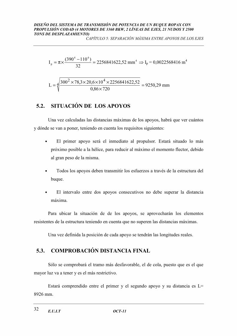
5.3. COMPROBACIÓN DISTANCIA FINAL
Sólo se comprobará el tramo más desfavorable, el de cola, puesto que es el que
mayor luz va a tener y es el más restrictivo.
Estará comprendido entre el primer y el segundo apoyo y su distancia es L=
8926 mm.
DISEÑO DEL SISTEMA DE TRANSMISIÓN DE POTENCIA DE UN BUQUE ROPAX CON PROPULSIÓN CODAD (4 MOTORES DE 3360 BKW, 2 LÍNEAS DE EJES, 21 NUDOS Y 2500 TONS DE DESPLAZAMIENTO)
CAPÍTULO 5: SEPARACIÓN MÁXIMA ENTRE APOYOS DE LOS EJES
E.U.I.T OCT-11 33
Si este tramo cumple los requisitos de Whirling y de tensión combinada el resto
de tramos también lo harán.
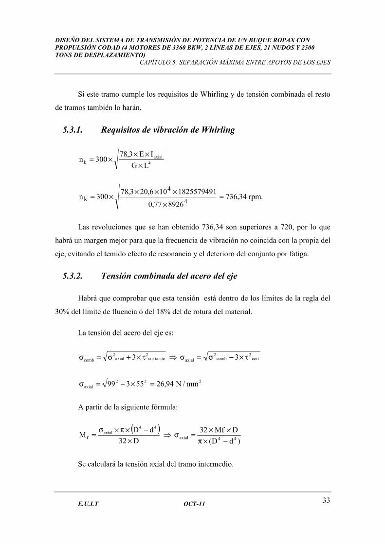
5.3.1. Requisitos de vibración de Whirling
4axial
kLG
IE3,78300n
×
×××=
.rpm34,736892677,0
1825579491106,203,78300n
4
4
k =×
××××=
Las revoluciones que se han obtenido 736,34 son superiores a 720, por lo que
habrá un margen mejor para que la frecuencia de vibración no coincida con la propia del
eje, evitando el temido efecto de resonancia y el deterioro del conjunto por fatiga.
5.3.2. Tensión combinada del acero del eje
Habrá que comprobar que esta tensión está dentro de los límites de la regla del
30% del límite de fluencia ó del 18% del de rotura del material.
La tensión del acero del eje es:
tetancor2
axial2
comb 3 τ×+σ=σ ⇒ cort2
comb2
axial 3 τ×−σ=σ
222axial mm/N94,2655399 =×−=σ
A partir de la siguiente fórmula:
( )D32
dDM
44axial
f×
−×π×σ= ⇒
)dD(
DMf3244axial
−×π
××=σ
Se calculará la tensión axial del tramo intermedio.
DISEÑO DEL SISTEMA DE TRANSMISIÓN DE POTENCIA DE UN BUQUE ROPAX CON PROPULSIÓN CODAD (4 MOTORES DE 3360 BKW, 2 LÍNEAS DE EJES, 21 NUDOS Y 2500 TONS DE DESPLAZAMIENTO)
CAPÍTULO 5: SEPARACIÓN MÁXIMA ENTRE APOYOS DE LOS EJES
E.U.I.T OCT-11 34
Donde:
• Mf = momento flector
• D = diámetro exterior del tramo de eje
• d = diámetro interior del tramo de eje
El momento flector se hallará mediante la fórmula:
8
lpMf
2×
=
Ya que la condición de nuestro eje es similar a la de una viga biapoyada
Donde:
• p = peso por metro lineal (N/m)
• l = longitud de la viga (m)
El peso por metro lineal del tramo dado se determinará con la fórmula:
gAm
peso××ρ=
Donde:
• ρ = densidad acero 7850 Kg/m3
• A = área de la sección del eje mm2
• g = gravedad 9,81m/s2
DISEÑO DEL SISTEMA DE TRANSMISIÓN DE POTENCIA DE UN BUQUE ROPAX CON PROPULSIÓN CODAD (4 MOTORES DE 3360 BKW, 2 LÍNEAS DE EJES, 21 NUDOS Y 2500 TONS DE DESPLAZAMIENTO)
CAPÍTULO 5: SEPARACIÓN MÁXIMA ENTRE APOYOS DE LOS EJES
E.U.I.T OCT-11 35
El área de una sección transversal del eje viene dado por:
4
dDA
22−
×π=
Así que:
222
mm04,737064
110370A =
−×π=
Con lo que se obtiene un peso por metro lineal de:
m/N2,754881,91039,806067850Peso 6 =×××= −
Por lo tanto, el momento flector es:
m/N04,673708
45,82,7548Mf
2
=×
=
Y la tensión axial:
)dD(
DMf3244axial
−×π
××=σ
2
44
3
axial mm/N65,13)110370(
3701004,6737032=
−×π
×××=σ
La tensión cortante viene dada por:
( )44cortdD
DMt16
−×π
××=τ
( )2
44
6
cort mm/N06,42110370
3701041516=
−×π
×××=τ

DISEÑO DEL SISTEMA DE TRANSMISIÓN DE POTENCIA DE UN BUQUE ROPAX CON PROPULSIÓN CODAD (4 MOTORES DE 3360 BKW, 2 LÍNEAS DE EJES, 21 NUDOS Y 2500 TONS DE DESPLAZAMIENTO)
CAPÍTULO 5: SEPARACIÓN MÁXIMA ENTRE APOYOS DE LOS EJES
E.U.I.T OCT-11 36
La tensión combinada viene dada por:
tetancor2
axial2
comb 3 τ×+σ=σ
Así que:
222comb mm/N12,7406,42365,13 =×+=σ
Comprobaremos si está dentro de los límites:
• 30% de 330 N/mm2 = 99 N/mm2 ⇒ 99 > 74,12
• 18% de 600 N/ mm2 = 108 N/ mm2 ⇒ 108 > 74,12
Luego la tensión combinada del material está dentro de las restricciones
impuestas. Por lo tanto es válida la longitud de eje seleccionada.
5.4. COMPROBACIÓN DE LA FRECUENCIA NATURAL A
TRAVÉS DE BUREAU VERITAS
Es importante analizar lo que indica la sociedad clasificadora del buque en
relación a la frecuencia natural. La Sociedad de Clasificación utilizada no tiene
especificado un método concreto para este cálculo, por lo que se ha optado por la
Sociedad de Clasificación Bureau Veritas de reconocido prestigio.
Según esta sociedad de clasificación la frecuencia natural viene expresada como:
4n
n lµ
IE
π2
af
×
××
×=
Donde:
• an = Constante según tabla 5.1
DISEÑO DEL SISTEMA DE TRANSMISIÓN DE POTENCIA DE UN BUQUE ROPAX CON PROPULSIÓN CODAD (4 MOTORES DE 3360 BKW, 2 LÍNEAS DE EJES, 21 NUDOS Y 2500 TONS DE DESPLAZAMIENTO)
CAPÍTULO 5: SEPARACIÓN MÁXIMA ENTRE APOYOS DE LOS EJES
E.U.I.T OCT-11 37
• E = Módulo de Young (N/m2)
• l = Longitud de la viga (m)
• I = Momento de inercia lateral (m4)
• µ = Masa por unidad de longitud (Kg/m)
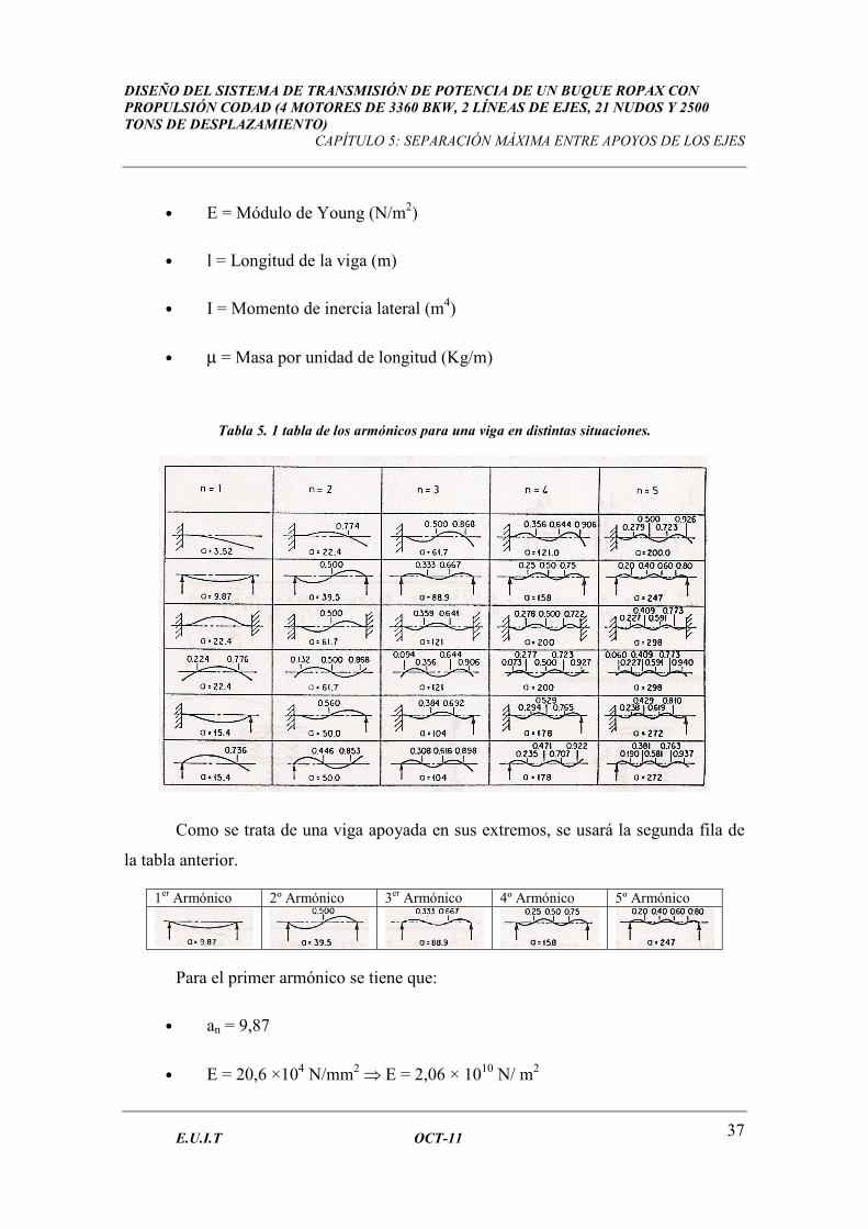
Tabla 5. 1 tabla de los armónicos para una viga en distintas situaciones.
Como se trata de una viga apoyada en sus extremos, se usará la segunda fila de
la tabla anterior.
1er Armónico 2º Armónico 3er Armónico 4º Armónico 5º Armónico
Para el primer armónico se tiene que:
• an = 9,87
• E = 20,6 ×10⁴ N/mm2 ⇒ E = 2,06 × 10¹⁰ N/ m2
DISEÑO DEL SISTEMA DE TRANSMISIÓN DE POTENCIA DE UN BUQUE ROPAX CON PROPULSIÓN CODAD (4 MOTORES DE 3360 BKW, 2 LÍNEAS DE EJES, 21 NUDOS Y 2500 TONS DE DESPLAZAMIENTO)
CAPÍTULO 5: SEPARACIÓN MÁXIMA ENTRE APOYOS DE LOS EJES
E.U.I.T OCT-11 38
• l = 8,926 m
• I = 0,0022568416 m4 ⇒ I = 2256841622,52 × 10-12 m4
• µ = 863,15 Kg/m
Luego:
Hz38159268769,44
10182557949110206
π2
9,87f
4
1210
n ,,
=×
××××
×=
−
Los armónicos restantes se han calculado de manera análoga.
Tabla 5. 2 Frecuencia en Hz y rpm para los distintos armónicos
Eje de cola 1er Armónico 2º Armónico 3er Armónico 4º Armónico 5º Armónico
Frecuencia (Hz) 15,38 61,55 138,53 246,21 384,9
Frecuencia (rpm)6 922,8 3693 8311,8 14772,6 23094
Las frecuencias naturales de los armónicos (922,8 rpm)están muy alejadas de las
600 rpm que es la frecuencia natural del eje. Luego las longitudes de separación de
apoyos propuestas son válidas ya que nunca entrarán en resonancia.
5.5. CÁLCULO DE VIBRACIÓN AXIAL POR LLOYD`S
REGISTER
Hay que comprobar que la velocidad crítica de vibración axial sea mayor que la
frecuencia natural del eje. Calculémosla:
6 La frecuencia en rpm se ha obtenidos multiplicando los Hertzios por 60.
DISEÑO DEL SISTEMA DE TRANSMISIÓN DE POTENCIA DE UN BUQUE ROPAX CON PROPULSIÓN CODAD (4 MOTORES DE 3360 BKW, 2 LÍNEAS DE EJES, 21 NUDOS Y 2500 TONS DE DESPLAZAMIENTO)
CAPÍTULO 5: SEPARACIÓN MÁXIMA ENTRE APOYOS DE LOS EJES
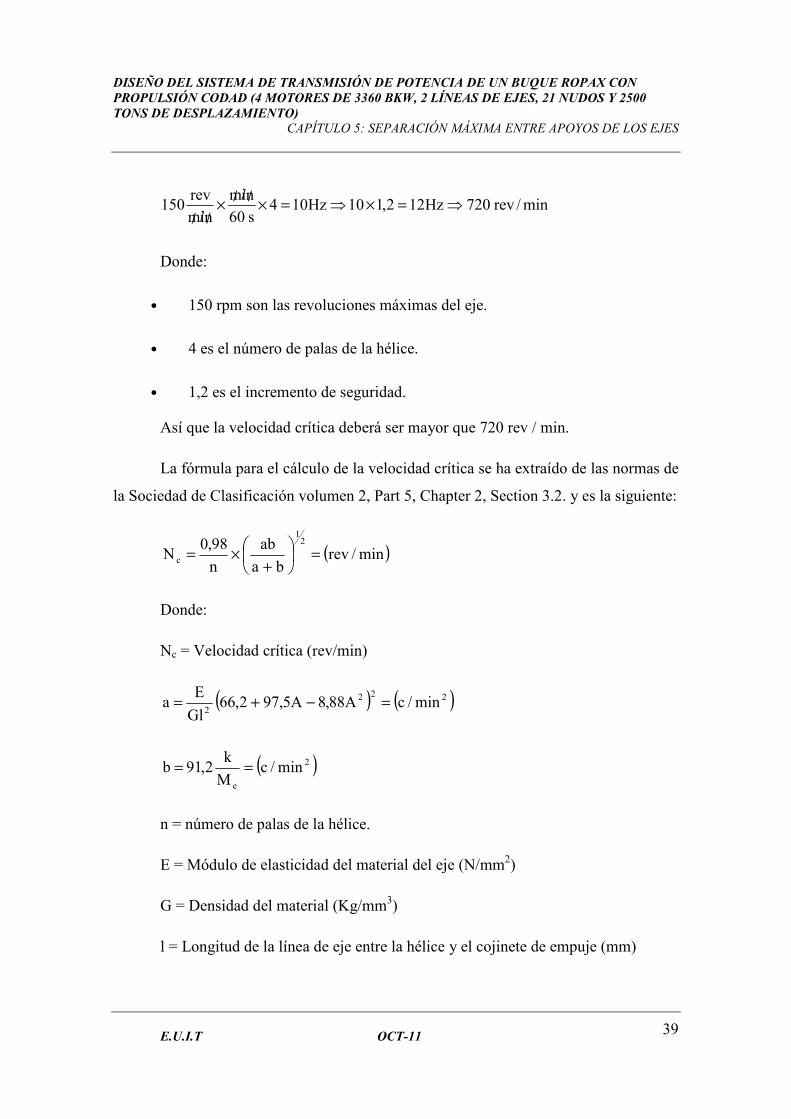
E.U.I.T OCT-11 39
min/rev720Hz122,110Hz104s60
nim
nim
rev150 ⇒=×⇒=×
///×
///
Donde:
• 150 rpm son las revoluciones máximas del eje.
• 4 es el número de palas de la hélice.
• 1,2 es el incremento de seguridad.
Así que la velocidad crítica deberá ser mayor que 720 rev / min.
La fórmula para el cálculo de la velocidad crítica se ha extraído de las normas de
la Sociedad de Clasificación volumen 2, Part 5, Chapter 2, Section 3.2. y es la siguiente:
( )min/revba
ab
n
98,0N
21
c =
+×=
Donde:
Nc = Velocidad crítica (rev/min)
( ) ( )222
2min/cA88,8A5,972,66
Gl
Ea =−+=
( )2
e
min/cM
k2,91b ==
n = número de palas de la hélice.
E = Módulo de elasticidad del material del eje (N/mm2)
G = Densidad del material (Kg/mm3)
l = Longitud de la línea de eje entre la hélice y el cojinete de empuje (mm)
DISEÑO DEL SISTEMA DE TRANSMISIÓN DE POTENCIA DE UN BUQUE ROPAX CON PROPULSIÓN CODAD (4 MOTORES DE 3360 BKW, 2 LÍNEAS DE EJES, 21 NUDOS Y 2500 TONS DE DESPLAZAMIENTO)
CAPÍTULO 5: SEPARACIÓN MÁXIMA ENTRE APOYOS DE LOS EJES
E.U.I.T OCT-11 40
A = M
m
M = peso de la hélice (Kg)
m = 0,785 x (D2 – d2) x G x l = masa del eje considerada en Kg
D = Diámetro exterior (mm)
d = Diámetro interior (mm)
Me = M x (A + 2)
k = rigidez cojinete de empuje (N/m)
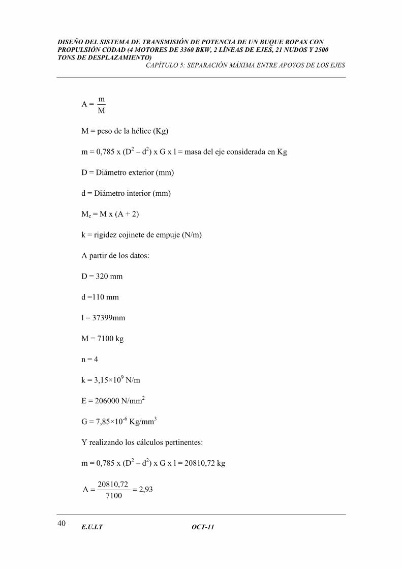
A partir de los datos:
D = 320 mm
d =110 mm
l = 37399mm
M = 7100 kg
n = 4
k = 3,15×10⁹ N/m
E = 206000 N/mm2
G = 7,85×10⁻⁶ Kg/mm3
Y realizando los cálculos pertinentes:
m = 0,785 x (D2 – d2) x G x l = 20810,72 kg
93,27100
20810,72A ==
DISEÑO DEL SISTEMA DE TRANSMISIÓN DE POTENCIA DE UN BUQUE ROPAX CON PROPULSIÓN CODAD (4 MOTORES DE 3360 BKW, 2 LÍNEAS DE EJES, 21 NUDOS Y 2500 TONS DE DESPLAZAMIENTO)
CAPÍTULO 5: SEPARACIÓN MÁXIMA ENTRE APOYOS DE LOS EJES
E.U.I.T OCT-11 41
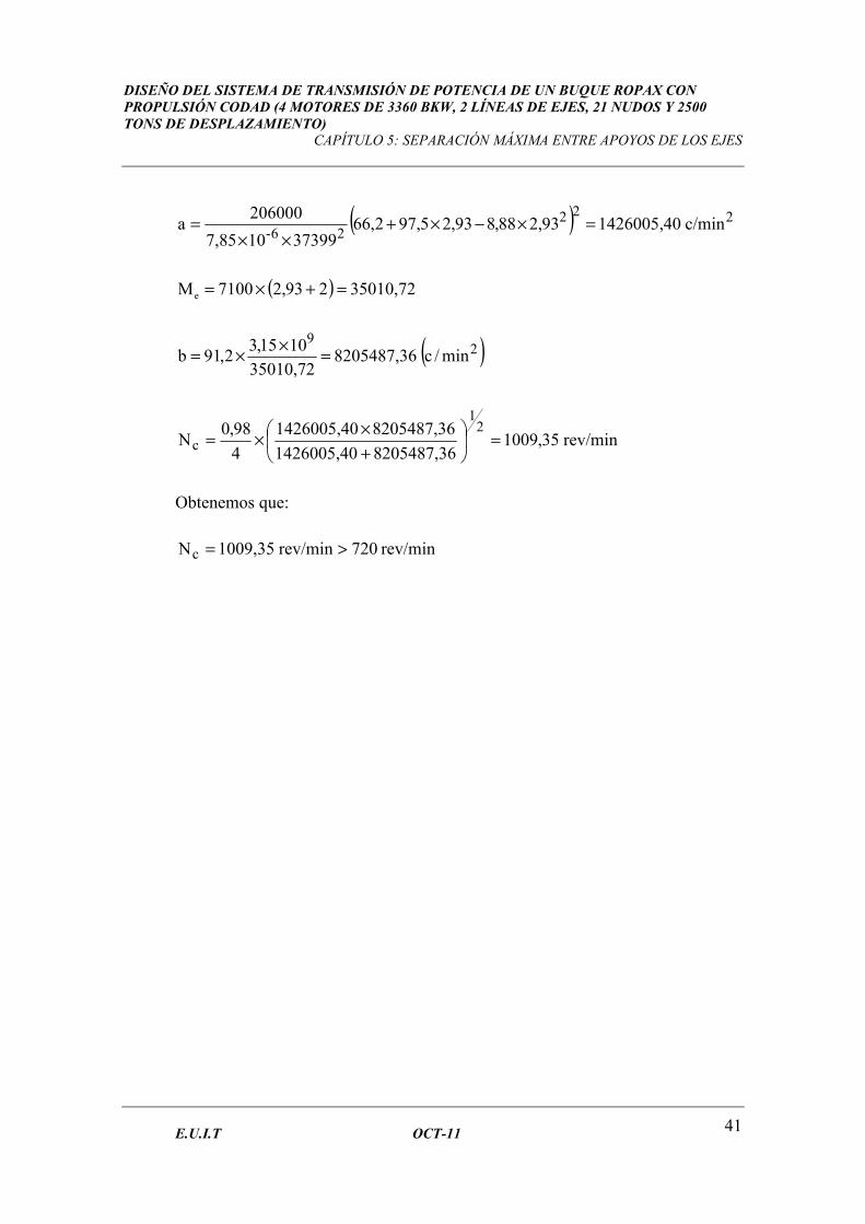
( ) 22226-
c/min1426005,4093,288,893,25,972,6637399107,85
206000a =×−×+
××=
( ) 35010,72293,27100Me =+×=
( )29
min/c8205487,3672,35010
1015,32,91b =
××=
rev/min35,00918205487,361426005,40
8205487,361426005,40
4
98,0N
21
c =
+
××=
Obtenemos que:
rev/min 720rev/min1009,35Nc >=

DISEÑO DEL SISTEMA DE TRANSMISIÓN DE POTENCIA DE UN BUQUE ROPAX CON PROPULSIÓN CODAD (4 MOTORES DE 3360 BKW, 2 LÍNEAS DE EJES, 21 NUDOS Y 2500 TONS DE DESPLAZAMIENTO)
CAPÍTULO 6: CÁLCULO DE LAS UNIONES DE LOS EJES DE TRANSMISIÓN
E.U.I.T OCT-11 43
CAPÍTULO 6. CÁLCULO DE LAS UNIONES DE LOS
EJES DE LA TRANSMISIÓN
El diseño de los acoplamientos se hará desde el punto de vista estructural o
resistente, utilizando los mismos criterios dimensionales usados en el diseño de los ejes
que acoplan y de forma que no reduzcan la capacidad mecánica de la transmisión. En
consecuencia, los acoplamientos podrán soportar y transmitir íntegramente todos los
esfuerzos a los que se ven sometidos los ejes que conecta.
Por lo anterior, podemos asegurar que el montaje entre eje y acoplamiento es
realizado de manera que la “unión” garantiza la transmisión de los esfuerzos recíprocos
entre ejes y acoplamientos y viceversa.
En función del nivel de las solicitaciones que actúen entre los elementos unidos,
las prestaciones estructurales de la unión serán más o menos exigentes. La elección final
del tipo de unión a utilizar debe realizarse considerando condiciones del contorno como:
• Espacio disponible.
• Facilidad de montaje y desmontaje.
• Frecuencia de desmontaje.
• Rapidez de montaje y desmontaje.
• Fiabilidad.
DISEÑO DEL SISTEMA DE TRANSMISIÓN DE POTENCIA DE UN BUQUE ROPAX CON PROPULSIÓN CODAD (4 MOTORES DE 3360 BKW, 2 LÍNEAS DE EJES, 21 NUDOS Y 2500 TONS DE DESPLAZAMIENTO)
CAPÍTULO 6: CÁLCULO DE LAS UNIONES DE LOS EJES DE TRANSMISIÓN
E.U.I.T OCT-11 44
6.1. TIPOS DE ACOPLAMIENTOS
6.1.1. Acoplamientos Rígidos
Se caracterizan porque transmiten íntegramente los esfuerzos de flexión y los
axiales que se apliquen a los ejes que acoplan. Por tanto, transmiten íntegramente los
movimientos permitidos al eje.
Se utilizan principalmente en los siguientes casos:
• Ejes con velocidades de rotación medias o bajas.
• Las máquinas que conectan son soportadas rígidamente.
• Se necesita de alineación muy precisa que se debe de mantener durante la
operación de trabajo.
• Estabilidad térmica, es decir ausencia de pequeñas dilataciones relativas.
6.1.2. Acoplamientos flexibles
En este tipo de acoplamiento no se transmiten íntegramente los esfuerzos de
flexión y/o axiales que se apliquen a los ejes y por tanto, no transmiten íntegramente los
movimientos relativos entre los ejes (o máquinas) que conectan, absorbiendo parcial o
totalmente dichos movimientos. La alineación requerida es menos precisa.
Podemos destacar como principales casos de utilización:
• Conectando máquinas con soportado elástico.
• Cuando las máquinas están sobre una base poco rígida.
DISEÑO DEL SISTEMA DE TRANSMISIÓN DE POTENCIA DE UN BUQUE ROPAX CON PROPULSIÓN CODAD (4 MOTORES DE 3360 BKW, 2 LÍNEAS DE EJES, 21 NUDOS Y 2500 TONS DE DESPLAZAMIENTO)
CAPÍTULO 6: CÁLCULO DE LAS UNIONES DE LOS EJES DE TRANSMISIÓN
E.U.I.T OCT-11 45
6.1.3. Acoplamientos torsioelásticos
Son acoplamientos flexibles a torsión exclusivamente o simultáneamente con
flexibilidad axial, y/o radial, y/o angular. Son, por tanto, acoplamientos que
transmitiendo íntegramente el par torsor estacionario adquieren por acción de éste una
deformación torsional elástica significativamente mayor que la de los ejes que acoplan.
Atendiendo al principio básico de diseño podemos decir que las uniones entre
ejes derivan de alguno de los tres tipos siguientes:
• Basadas en efectos de forma.
• Por inserción de elementos de bloqueo.
• Por la acción de fuerzas de rozamiento.
6.2. TIPOS DE UNIONES BASADAS EN EL EFECTO DE
FORMA
6.2.1. Unión Estriada
Ambos ejes quedan torsionalmente conectados por contacto entre las diversas
acanaladuras formadas por los correspondientes estriados macho de un eje y hembra del
otro. En este caso, las uniones estriadas mantienen en todo momento el contacto entre
todos y cada uno de sus dientes, transmitiendo el par torsor sin que exista movimiento
relativo entre ellos.
La ausencia de fricción hace innecesaria la lubricación de este tipo de unión.

DISEÑO DEL SISTEMA DE TRANSMISIÓN DE POTENCIA DE UN BUQUE ROPAX CON PROPULSIÓN CODAD (4 MOTORES DE 3360 BKW, 2 LÍNEAS DE EJES, 21 NUDOS Y 2500 TONS DE DESPLAZAMIENTO)
CAPÍTULO 6: CÁLCULO DE LAS UNIONES DE LOS EJES DE TRANSMISIÓN
E.U.I.T OCT-11 46
Figura 6. 1 Unión estriada
Apuntes Cálculo Estructural
6.2.2. Por inserción de elementos de bloqueo
6.2.2.1. Unión de bridas empernadas
Es la unión más común y tradicional en la construcción naval. La unión es
simple y consiste en enfrentar las bridas o platos a unir, realizándose a ambos taladros
pasantes, diametralmente opuestos, del mismo diámetro concéntrico al que se ajustan
los pernos. Éstos deben ser perpendiculares a la superficie de contacto entre bridas. Los
pernos transmiten el par torsor trabajando a esfuerzo cortante.
Figura 6. 2 Bridas empernadas
Apuntes Cálculo Estructural
DISEÑO DEL SISTEMA DE TRANSMISIÓN DE POTENCIA DE UN BUQUE ROPAX CON PROPULSIÓN CODAD (4 MOTORES DE 3360 BKW, 2 LÍNEAS DE EJES, 21 NUDOS Y 2500 TONS DE DESPLAZAMIENTO)
CAPÍTULO 6: CÁLCULO DE LAS UNIONES DE LOS EJES DE TRANSMISIÓN
E.U.I.T OCT-11 47
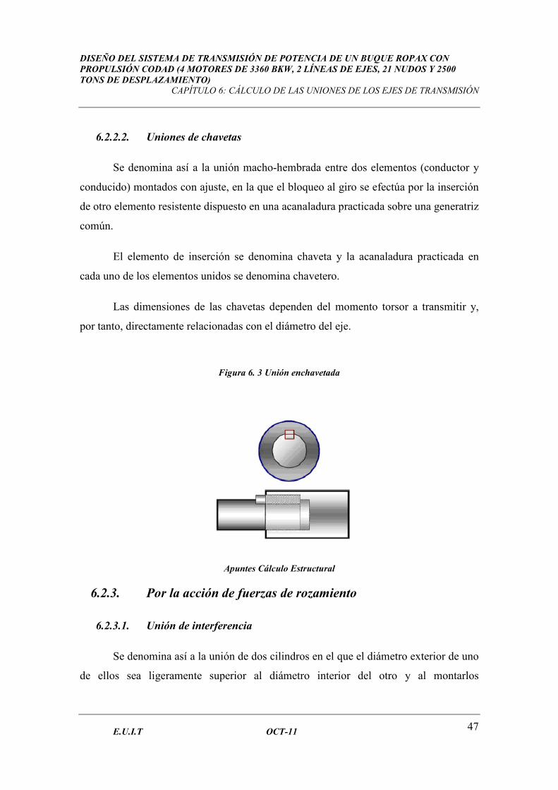
6.2.2.2. Uniones de chavetas
Se denomina así a la unión macho-hembrada entre dos elementos (conductor y
conducido) montados con ajuste, en la que el bloqueo al giro se efectúa por la inserción
de otro elemento resistente dispuesto en una acanaladura practicada sobre una generatriz
común.
El elemento de inserción se denomina chaveta y la acanaladura practicada en
cada uno de los elementos unidos se denomina chavetero.
Las dimensiones de las chavetas dependen del momento torsor a transmitir y,
por tanto, directamente relacionadas con el diámetro del eje.
Figura 6. 3 Unión enchavetada
Apuntes Cálculo Estructural
6.2.3. Por la acción de fuerzas de rozamiento
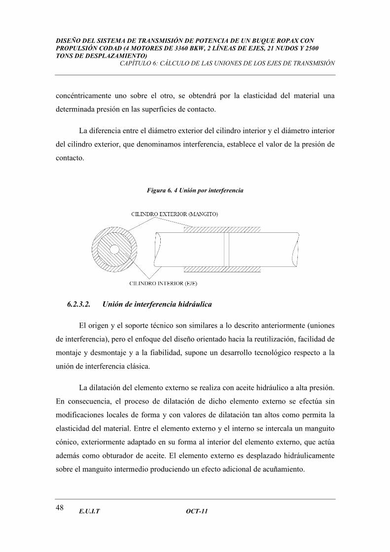
6.2.3.1. Unión de interferencia
Se denomina así a la unión de dos cilindros en el que el diámetro exterior de uno
de ellos sea ligeramente superior al diámetro interior del otro y al montarlos
DISEÑO DEL SISTEMA DE TRANSMISIÓN DE POTENCIA DE UN BUQUE ROPAX CON PROPULSIÓN CODAD (4 MOTORES DE 3360 BKW, 2 LÍNEAS DE EJES, 21 NUDOS Y 2500 TONS DE DESPLAZAMIENTO)
CAPÍTULO 6: CÁLCULO DE LAS UNIONES DE LOS EJES DE TRANSMISIÓN
E.U.I.T OCT-11 48
concéntricamente uno sobre el otro, se obtendrá por la elasticidad del material una
determinada presión en las superficies de contacto.
La diferencia entre el diámetro exterior del cilindro interior y el diámetro interior
del cilindro exterior, que denominamos interferencia, establece el valor de la presión de
contacto.
Figura 6. 4 Unión por interferencia
6.2.3.2. Unión de interferencia hidráulica
El origen y el soporte técnico son similares a lo descrito anteriormente (uniones
de interferencia), pero el enfoque del diseño orientado hacia la reutilización, facilidad de
montaje y desmontaje y a la fiabilidad, supone un desarrollo tecnológico respecto a la
unión de interferencia clásica.
La dilatación del elemento externo se realiza con aceite hidráulico a alta presión.
En consecuencia, el proceso de dilatación de dicho elemento externo se efectúa sin
modificaciones locales de forma y con valores de dilatación tan altos como permita la
elasticidad del material. Entre el elemento externo y el interno se intercala un manguito
cónico, exteriormente adaptado en su forma al interior del elemento externo, que actúa
además como obturador de aceite. El elemento externo es desplazado hidráulicamente
sobre el manguito intermedio produciendo un efecto adicional de acuñamiento.
DISEÑO DEL SISTEMA DE TRANSMISIÓN DE POTENCIA DE UN BUQUE ROPAX CON PROPULSIÓN CODAD (4 MOTORES DE 3360 BKW, 2 LÍNEAS DE EJES, 21 NUDOS Y 2500 TONS DE DESPLAZAMIENTO)
CAPÍTULO 6: CÁLCULO DE LAS UNIONES DE LOS EJES DE TRANSMISIÓN
E.U.I.T OCT-11 49
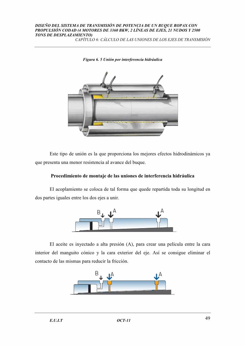
Figura 6. 5 Unión por interferencia hidráulica
Este tipo de unión es la que proporciona los mejores efectos hidrodinámicos ya
que presenta una menor resistencia al avance del buque.
Procedimiento de montaje de las uniones de interferencia hidráulica
El acoplamiento se coloca de tal forma que quede repartida toda su longitud en
dos partes iguales entre los dos ejes a unir.
El aceite es inyectado a alta presión (A), para crear una película entre la cara
interior del manguito cónico y la cara exterior del eje. Así se consigue eliminar el
contacto de las mismas para reducir la fricción.
DISEÑO DEL SISTEMA DE TRANSMISIÓN DE POTENCIA DE UN BUQUE ROPAX CON PROPULSIÓN CODAD (4 MOTORES DE 3360 BKW, 2 LÍNEAS DE EJES, 21 NUDOS Y 2500 TONS DE DESPLAZAMIENTO)
CAPÍTULO 6: CÁLCULO DE LAS UNIONES DE LOS EJES DE TRANSMISIÓN
E.U.I.T OCT-11 50
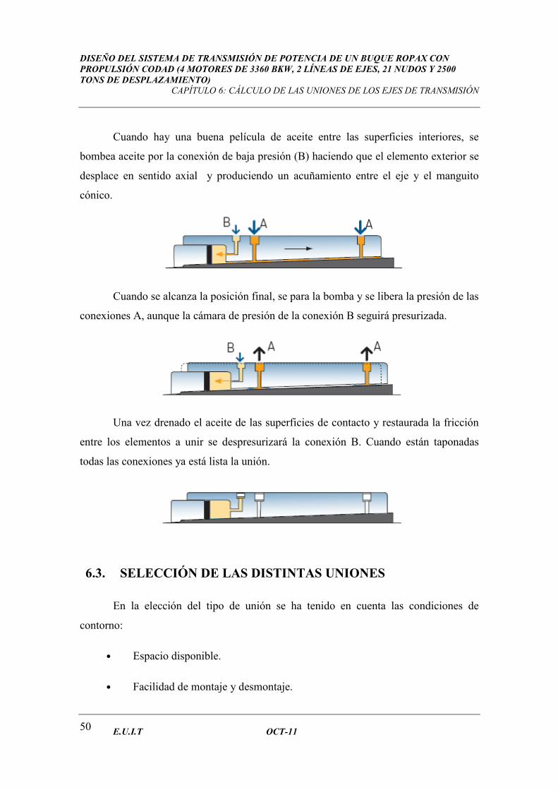
Cuando hay una buena película de aceite entre las superficies interiores, se
bombea aceite por la conexión de baja presión (B) haciendo que el elemento exterior se
desplace en sentido axial y produciendo un acuñamiento entre el eje y el manguito
cónico.
Cuando se alcanza la posición final, se para la bomba y se libera la presión de las
conexiones A, aunque la cámara de presión de la conexión B seguirá presurizada.
Una vez drenado el aceite de las superficies de contacto y restaurada la fricción
entre los elementos a unir se despresurizará la conexión B. Cuando están taponadas
todas las conexiones ya está lista la unión.
6.3. SELECCIÓN DE LAS DISTINTAS UNIONES
En la elección del tipo de unión se ha tenido en cuenta las condiciones de
contorno:
• Espacio disponible.
• Facilidad de montaje y desmontaje.
DISEÑO DEL SISTEMA DE TRANSMISIÓN DE POTENCIA DE UN BUQUE ROPAX CON PROPULSIÓN CODAD (4 MOTORES DE 3360 BKW, 2 LÍNEAS DE EJES, 21 NUDOS Y 2500 TONS DE DESPLAZAMIENTO)
CAPÍTULO 6: CÁLCULO DE LAS UNIONES DE LOS EJES DE TRANSMISIÓN
E.U.I.T OCT-11 51
• Frecuencia de desmontaje.
• Rapidez de montaje y desmontaje.
• Fiabilidad.
Y los elementos a unir:
• Del tipo eje a eje
• Tramo de proa a tramo intermedio
• Tramo intermedio a tramo de cola
• Eje a reductor
• Reductor a motor propulsor
Las uniones de los tramos de eje a eje y la brida del eje al reductor, serán por
interferencia hidráulica. En su elección se tendrá en cuenta el diámetro exterior del eje a
unir y el par torsor a transmitir.
La unión de la brida del eje a la brida del reductor se hará mediante tornillos.
Las distintas uniones se elegirán de las tablas contenidas en el anexo y han sido
obtenidas del catálogo OK shaft coupling de la casa SKF.
6.3.1. Unión eje/eje
6.3.1.1. Tramo de proa a tramo intermedio
Para la unión de eje a eje se usarán las del tipo OKC, seleccionando el más
adecuado en el catálogo del anexo.
DISEÑO DEL SISTEMA DE TRANSMISIÓN DE POTENCIA DE UN BUQUE ROPAX CON PROPULSIÓN CODAD (4 MOTORES DE 3360 BKW, 2 LÍNEAS DE EJES, 21 NUDOS Y 2500 TONS DE DESPLAZAMIENTO)
CAPÍTULO 6: CÁLCULO DE LAS UNIONES DE LOS EJES DE TRANSMISIÓN
E.U.I.T OCT-11 52
Teniendo en cuenta el par máximo a transmitir más un 30% de margen de
seguridad, 539,5 kN×m, y el diámetro exterior del tramo de proa, 320 mm, se elegirá
OKC 320 ya que el par torsor máximo que puede trasmitir es de 852 kN×m que es
superior al necesario.
6.3.1.2. Tramo intermedio a tramo de cola
En la elección de este tramo se han usado los mismos criterios que en el anterior,
pero con los datos:
Momento torsor = 539,5 kN×m
Diámetro exterior = 370 mm
Se elegirá el acoplamiento OKC 370 que puede transmitir un par torsor de 1320
kN×m superior al necesario.
6.3.2. Unión eje/reductor
En esta unión un extremo se fijará al eje por presión hidráulica y el otro extremo
se unirá a la brida del reductor mediante pernos. El cálculo de estos últimos se verá
detalladamente en el siguiente capítulo.
Para la elegir la unión, se ha seguido el mismo criterio anterior pero usando la
tabla OKF 310-700 y con los datos:
Momento torsor = 539,5 kN×m
Diámetro exterior = 320 mm
Se elegirá el acoplamiento OKF 320, con capacidad de transmitir un par torsor
de 852 kN×m, superior al necesario.
DISEÑO DEL SISTEMA DE TRANSMISIÓN DE POTENCIA DE UN BUQUE ROPAX CON PROPULSIÓN CODAD (4 MOTORES DE 3360 BKW, 2 LÍNEAS DE EJES, 21 NUDOS Y 2500 TONS DE DESPLAZAMIENTO)
CAPÍTULO 6: CÁLCULO DE LAS UNIONES DE LOS EJES DE TRANSMISIÓN
E.U.I.T OCT-11 53
6.3.3. Acoplamiento entre motor propulsor y reductor
Entre el motor y el reductor se usará un acoplamiento del tipo torsioelástico, de
la casa Vulkan, que es capaz de absorber las desviaciones axiales, angulares y
torsionales.
El momento máximo a transmitir deberá ser menor o igual que el par nominal
del acoplamiento.
El momento máximo viene dado por:
rpm
kW55,9Mt
×=
Para kW= 3360 y rpm= 150, se obtiene que:
mkN78,42750
336055,9Mt ×=
×=
Teniendo este dato en cuenta, se elegirá el acoplamiento RATO R G 312Z R, del
catálogo que se muestra en el anexo, con un par nominal de 50 kN×m, con
desplazamientos axial y radial de 7 y 17 mm, respectivamente.


DISEÑO DEL SISTEMA DE TRANSMISIÓN DE POTENCIA DE UN BUQUE ROPAX CON PROPULSIÓN CODAD (4 MOTORES DE 3360 BKW, 2 LÍNEAS DE EJES, 21 NUDOS Y 2500 TONS DE DESPLAZAMIENTO)
CAPÍTULO 7: CÁLCULO DE LA UNIÓN EMPERNADA
E.U.I.T OCT-11 55
CAPÍTULO 7. CÁLCULO DE LA UNIÓN
EMPERNADA
7.1. DATOS DE LA BRIDA DEL REDUCTOR
Se propone una brida de salida de potencia del reductor con las siguientes
características:
Número de taladros 8
Diámetro de los taladros 64 mm
Diámetro entre taladros 592,6 mm
Espesor de la brida 64 mm
7.2. DIMENSIONES DE LA ARANDELA SEGÚN ISO 7089
Atendiendo a la norma ISO 7089, las arandelas serán ISO 7089-64 HV 200.
Figura 7. 1 Arandela ISO 7089
Norma ISO 7089
DISEÑO DEL SISTEMA DE TRANSMISIÓN DE POTENCIA DE UN BUQUE ROPAX CON PROPULSIÓN CODAD (4 MOTORES DE 3360 BKW, 2 LÍNEAS DE EJES, 21 NUDOS Y 2500 TONS DE DESPLAZAMIENTO)
CAPÍTULO 7: CÁLCULO DE LA UNIÓN EMPERNADA
E.U.I.T OCT-11 56
Tabla 7. 1 Dimensiones arandela 64 HV 200
Clearance
d1
Outside diameter
d2
Thickness
h Nominal size
(Nominal thread diameter, d) nom (mín) máx nom (máx) mín nom máx mín
64 mm 70 mm 70,4 mm 115 mm 113,6 mm 10 mm 11 mm 9 mm
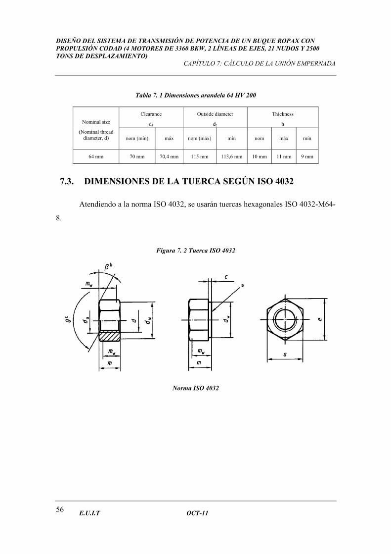
7.3. DIMENSIONES DE LA TUERCA SEGÚN ISO 4032
Atendiendo a la norma ISO 4032, se usarán tuercas hexagonales ISO 4032-M64-
8.
Figura 7. 2 Tuerca ISO 4032
Norma ISO 4032
DISEÑO DEL SISTEMA DE TRANSMISIÓN DE POTENCIA DE UN BUQUE ROPAX CON PROPULSIÓN CODAD (4 MOTORES DE 3360 BKW, 2 LÍNEAS DE EJES, 21 NUDOS Y 2500 TONS DE DESPLAZAMIENTO)
CAPÍTULO 7: CÁLCULO DE LA UNIÓN EMPERNADA
E.U.I.T OCT-11 57
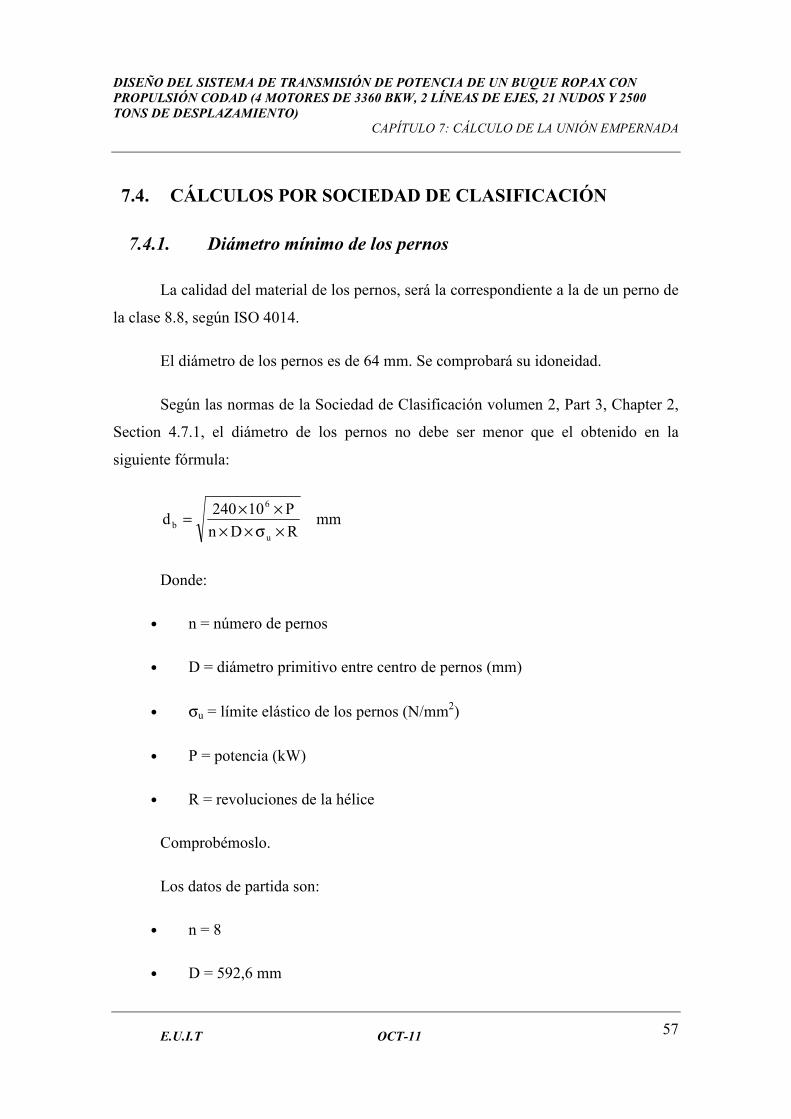
7.4. CÁLCULOS POR SOCIEDAD DE CLASIFICACIÓN
7.4.1. Diámetro mínimo de los pernos
La calidad del material de los pernos, será la correspondiente a la de un perno de
la clase 8.8, según ISO 4014.
El diámetro de los pernos es de 64 mm. Se comprobará su idoneidad.
Según las normas de la Sociedad de Clasificación volumen 2, Part 3, Chapter 2,
Section 4.7.1, el diámetro de los pernos no debe ser menor que el obtenido en la
siguiente fórmula:
mmRDn
P10240d
u
6
b×σ××
××=
Donde:
• n = número de pernos
• D = diámetro primitivo entre centro de pernos (mm)
• σu = límite elástico de los pernos (N/mm2)
• P = potencia (kW)
• R = revoluciones de la hélice
Comprobémoslo.
Los datos de partida son:
• n = 8
• D = 592,6 mm
DISEÑO DEL SISTEMA DE TRANSMISIÓN DE POTENCIA DE UN BUQUE ROPAX CON PROPULSIÓN CODAD (4 MOTORES DE 3360 BKW, 2 LÍNEAS DE EJES, 21 NUDOS Y 2500 TONS DE DESPLAZAMIENTO)
CAPÍTULO 7: CÁLCULO DE LA UNIÓN EMPERNADA
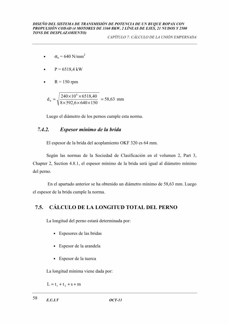
E.U.I.T OCT-11 58
• σu = 640 N/mm2
• P = 6518,4 kW
• R = 150 rpm
mm 58,63150640592,68
6518,4010240d
6
b =×××
××=
Luego el diámetro de los pernos cumple esta norma.
7.4.2. Espesor mínimo de la brida
El espesor de la brida del acoplamiento OKF 320 es 64 mm.
Según las normas de la Sociedad de Clasificación en el volumen 2, Part 3,
Chapter 2, Section 4.8.1, el espesor mínimo de la brida será igual al diámetro mínimo
del perno.
En el apartado anterior se ha obtenido un diámetro mínimo de 58,63 mm. Luego
el espesor de la brida cumple la norma.
7.5. CÁLCULO DE LA LONGITUD TOTAL DEL PERNO
La longitud del perno estará determinada por:
• Espesores de las bridas
• Espesor de la arandela
• Espesor de la tuerca
La longitud mínima viene dada por:
msttL 21 +++=
DISEÑO DEL SISTEMA DE TRANSMISIÓN DE POTENCIA DE UN BUQUE ROPAX CON PROPULSIÓN CODAD (4 MOTORES DE 3360 BKW, 2 LÍNEAS DE EJES, 21 NUDOS Y 2500 TONS DE DESPLAZAMIENTO)
CAPÍTULO 7: CÁLCULO DE LA UNIÓN EMPERNADA
E.U.I.T OCT-11 59
Donde:
t1 = espesor brida del reductor
t2 = espesor brida del eje
s = espesor de la arandela
m = espesor de la tuerca
Se usarán pernos de cabeza hexagonal ISO 4014-M64×260-8.8, arandelas ISO
7089-64 HV 200 y tuercas hexagonales ISO 4032-M64-8. Así que los datos son:
t1 = 64 mm
t2 = 64 mm
s = 10 mm
m = 51 mm
Luego la longitud mínima es:
mm18951106464L =+++=
Se usarán tornillos de 260 mm que son de una longitud mayor que la mínima
exigida.
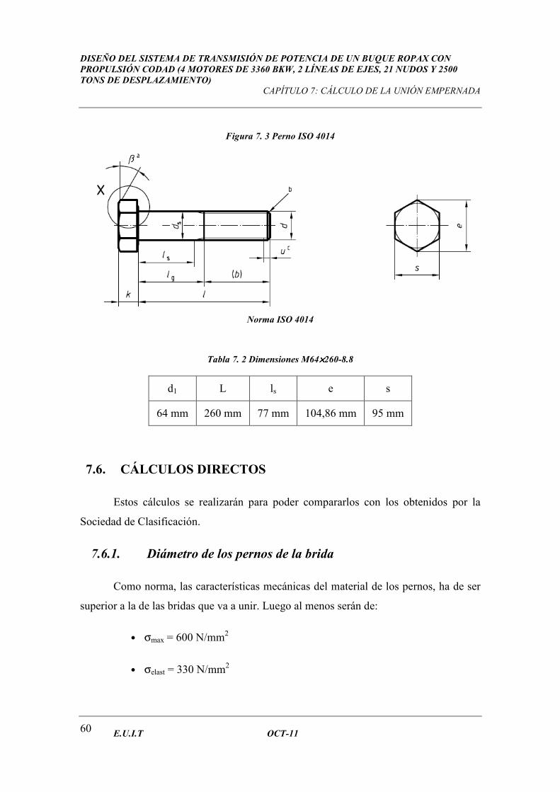
DISEÑO DEL SISTEMA DE TRANSMISIÓN DE POTENCIA DE UN BUQUE ROPAX CON PROPULSIÓN CODAD (4 MOTORES DE 3360 BKW, 2 LÍNEAS DE EJES, 21 NUDOS Y 2500 TONS DE DESPLAZAMIENTO)
CAPÍTULO 7: CÁLCULO DE LA UNIÓN EMPERNADA
E.U.I.T OCT-11 60
Figura 7. 3 Perno ISO 4014
Norma ISO 4014
Tabla 7. 2 Dimensiones M64××××260-8.8
d1 L ls e s
64 mm 260 mm 77 mm 104,86 mm 95 mm
7.6. CÁLCULOS DIRECTOS
Estos cálculos se realizarán para poder compararlos con los obtenidos por la
Sociedad de Clasificación.
7.6.1. Diámetro de los pernos de la brida
Como norma, las características mecánicas del material de los pernos, ha de ser
superior a la de las bridas que va a unir. Luego al menos serán de:
• σmax = 600 N/mm2
• σelast = 330 N/mm2
DISEÑO DEL SISTEMA DE TRANSMISIÓN DE POTENCIA DE UN BUQUE ROPAX CON PROPULSIÓN CODAD (4 MOTORES DE 3360 BKW, 2 LÍNEAS DE EJES, 21 NUDOS Y 2500 TONS DE DESPLAZAMIENTO)
CAPÍTULO 7: CÁLCULO DE LA UNIÓN EMPERNADA
E.U.I.T OCT-11 61
• τcort = 190,53 N/mm2
Los pernos que se utilizarán serán de la clase 8.8 y, según la ISO 898-1, sus
características mecánicas son:
• límite de rotura (σmax) = 800 N/mm2
• límite elástico 640 N/mm2
Sabemos que:
3elast
cort
σ=τ
Así que la τcort del perno clase 8.8 será:
2cort mm/N5,369
3
640==τ
En una unión de bridas empernadas, los pernos transmiten el par torsor
trabajando a esfuerzo cortante. La sección crítica del perno es la correspondiente a
4
d 2×π
. Luego el esfuerzo cortante que tienen que soportar los pernos viene dado por la
siguiente fórmula:
4
dnF
2per
perc ×π×τ×= (7.1)
Donde:
• nper = Número de pernos
• τ = Tensión cortante del perno
• dper = Diámetro de los pernos
DISEÑO DEL SISTEMA DE TRANSMISIÓN DE POTENCIA DE UN BUQUE ROPAX CON PROPULSIÓN CODAD (4 MOTORES DE 3360 BKW, 2 LÍNEAS DE EJES, 21 NUDOS Y 2500 TONS DE DESPLAZAMIENTO)
CAPÍTULO 7: CÁLCULO DE LA UNIÓN EMPERNADA
E.U.I.T OCT-11 62
Si DP es el diámetro entre centros de pernos, la capacidad de transmisión de par
torsor de los pernos trabajando a esfuerzo cortante es:
2
DFM pct ×= (7.2)
Despejando de Fc de (7.2):
p
tc D
2MF
×=
Y sustituyendo en (7.1) y operando convenientemente, se obtiene el esfuerzo
cortante máximo que puede soportar cada perno:
2perper
c
dn
4F
×π×
×=τ
Sabiendo que:
• nper = 8
• dp = 64 mm
• Dp = 592,6 mm
• Mt = 415 kN×m
Y haciendo los cálculos oportunos:
N 1400623,696,592
210415F
6
c =××
=
2
2N/mm 42,54
646
41400623,69=
×π×
×=τ
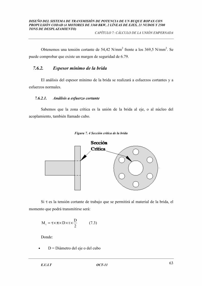
DISEÑO DEL SISTEMA DE TRANSMISIÓN DE POTENCIA DE UN BUQUE ROPAX CON PROPULSIÓN CODAD (4 MOTORES DE 3360 BKW, 2 LÍNEAS DE EJES, 21 NUDOS Y 2500 TONS DE DESPLAZAMIENTO)
CAPÍTULO 7: CÁLCULO DE LA UNIÓN EMPERNADA
E.U.I.T OCT-11 63
Obtenemos una tensión cortante de 54,42 N/mm2 frente a los 369,5 N/mm2. Se
puede comprobar que existe un margen de seguridad de 6.79.
7.6.2. Espesor mínimo de la brida
El análisis del espesor mínimo de la brida se realizará a esfuerzos cortantes y a
esfuerzos normales.
7.6.2.1. Análisis a esfuerzo cortante
Sabemos que la zona crítica es la unión de la brida al eje, o al núcleo del
acoplamiento, también llamado cubo.
Figura 7. 4 Sección crítica de la brida
Si τ es la tensión cortante de trabajo que se permitirá al material de la brida, el
momento que podrá transmitirse será:
2
DtDM t ×××π×τ= (7.3)
Donde:
• D = Diámetro del eje o del cubo
DISEÑO DEL SISTEMA DE TRANSMISIÓN DE POTENCIA DE UN BUQUE ROPAX CON PROPULSIÓN CODAD (4 MOTORES DE 3360 BKW, 2 LÍNEAS DE EJES, 21 NUDOS Y 2500 TONS DE DESPLAZAMIENTO)
CAPÍTULO 7: CÁLCULO DE LA UNIÓN EMPERNADA
E.U.I.T OCT-11 64
• t = espesor mínimo de la brida
Despejando “t” de (7.3), se tendrá el espesor mínimo:
2t
D
2Mt
×π×τ
×=
Los datos son:
• Mt = 415 kN×m
• τcort = 190,53 N/mm2
• D = 320 mm
Luego:
mm54,1332053,190
210*415t
2
6
=×π×
×=
7.6.2.2. Análisis a esfuerzo normal
Los esfuerzos normales se producirán en la superficie de contacto entre los
pernos y la brida.
Si σ es la tensión normal de trabajo que se permitirá al material de la brida, el
momento que podrá transmitirse será:
2
DntdM p
t ××××σ= (7.4)
Donde:
• d = diámetro de los pernos
• t = espesor de la brida
DISEÑO DEL SISTEMA DE TRANSMISIÓN DE POTENCIA DE UN BUQUE ROPAX CON PROPULSIÓN CODAD (4 MOTORES DE 3360 BKW, 2 LÍNEAS DE EJES, 21 NUDOS Y 2500 TONS DE DESPLAZAMIENTO)
CAPÍTULO 7: CÁLCULO DE LA UNIÓN EMPERNADA
E.U.I.T OCT-11 65
• n = número de pernos
• Dp = diámetro entre centro de pernos
Despejando “t” de (7.4), se tendrá el espesor mínimo:
p
t
Dnd
2Mt
×××σ
×=
Los datos son:
• Mt = 415 kN×m
• σ = 330 N/mm2
• d = 64 mm
• n = 8
• Dp = 592,6 mm
Luego:
mm 8,29 6,592864330
210415t
6
=×××
××=
Conclusión:
Según los datos obtenidos en el análisis tanto a cortante como a normal, se
tomará como espesor mínimo el de mayor valor, 13,54 mm, ya que con este espesor la
brida será capaz de soportar los esfuerzos normales y cortantes.

DISEÑO DEL SISTEMA DE TRANSMISIÓN DE POTENCIA DE UN BUQUE ROPAX CON PROPULSIÓN CODAD (4 MOTORES DE 3360 BKW, 2 LÍNEAS DE EJES, 21 NUDOS Y 2500 TONS DE DESPLAZAMIENTO)
CAPÍTULO 8: CÁLCULO DE LA SITUACIÓN DE LOS APOYOS
E.U.I.T OCT-11 67
CAPÍTULO 8. CÁLCULO DE LA SITUACIÓN DE
LOS APOYOS
A continuación se mostrará la situación más adecuada de los apoyos.
Los cálculos se han realizado con un software de resistencia de materiales
llamado DT Beam y teniendo en cuenta las características del eje.
Los segmentos de los ejes en los que se encuentran los acoplamientos se han
considerado como tramos de un diámetro mayor: el diámetro exterior del acoplamiento.
La situación de los apoyos se ha obtenido tras varias pruebas, modificando la
distancia de los apoyos que lo permitían.
Conocida estas distancias se obtendrán las reacciones que hay en cada apoyo, las
tensiones axiales, los esfuerzos cortantes y la flecha máxima (δ) entre dos apoyos
consecutivos.
8.1. DATOS DE PARTIDA PARA TRABAJAR CON SOFTWARE
Las unidades que se han usado para trabajar con el programa son las siguientes:
• Distancia entre los apoyos: mm
• Área: mm2
• Momentos de inercia: mm4
• Elasticidad del acero: kN/mm2
• Densidad del acero: kN/mm3
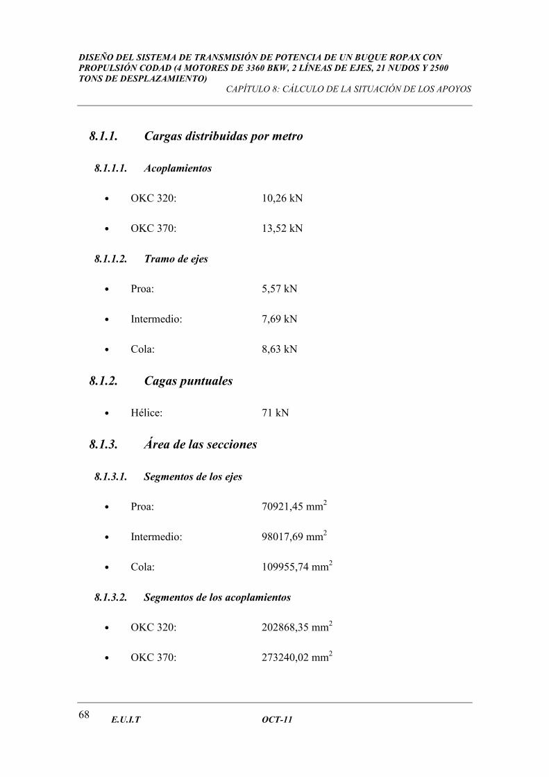
DISEÑO DEL SISTEMA DE TRANSMISIÓN DE POTENCIA DE UN BUQUE ROPAX CON PROPULSIÓN CODAD (4 MOTORES DE 3360 BKW, 2 LÍNEAS DE EJES, 21 NUDOS Y 2500 TONS DE DESPLAZAMIENTO)
CAPÍTULO 8: CÁLCULO DE LA SITUACIÓN DE LOS APOYOS
E.U.I.T OCT-11 68
8.1.1. Cargas distribuidas por metro
8.1.1.1. Acoplamientos
• OKC 320: 10,26 kN
• OKC 370: 13,52 kN
8.1.1.2. Tramo de ejes
• Proa: 5,57 kN
• Intermedio: 7,69 kN
• Cola: 8,63 kN
8.1.2. Cagas puntuales
• Hélice: 71 kN
8.1.3. Área de las secciones
8.1.3.1. Segmentos de los ejes
• Proa: 70921,45 mm2
• Intermedio: 98017,69 mm2
• Cola: 109955,74 mm2
8.1.3.2. Segmentos de los acoplamientos
• OKC 320: 202868,35 mm2
• OKC 370: 273240,02 mm2
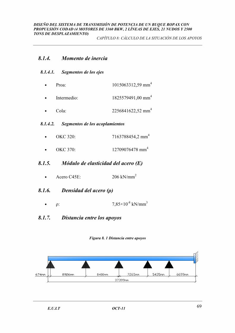
DISEÑO DEL SISTEMA DE TRANSMISIÓN DE POTENCIA DE UN BUQUE ROPAX CON PROPULSIÓN CODAD (4 MOTORES DE 3360 BKW, 2 LÍNEAS DE EJES, 21 NUDOS Y 2500 TONS DE DESPLAZAMIENTO)
CAPÍTULO 8: CÁLCULO DE LA SITUACIÓN DE LOS APOYOS
E.U.I.T OCT-11 69
8.1.4. Momento de inercia
8.1.4.1. Segmentos de los ejes
• Proa: 1015063312,59 mm4
• Intermedio: 1825579491,00 mm4
• Cola: 2256841622,52 mm4
8.1.4.2. Segmentos de los acoplamientos
• OKC 320: 7163788454,2 mm4
• OKC 370: 12709076478 mm4
8.1.5. Módulo de elasticidad del acero (E)
• Acero C45E: 206 kN/mm2
8.1.6. Densidad del acero (ρ)
• ρ: 7,85×10⁻⁸ kN/mm3
8.1.7. Distancia entre los apoyos
Figura 8. 1 Distancia entre apoyos
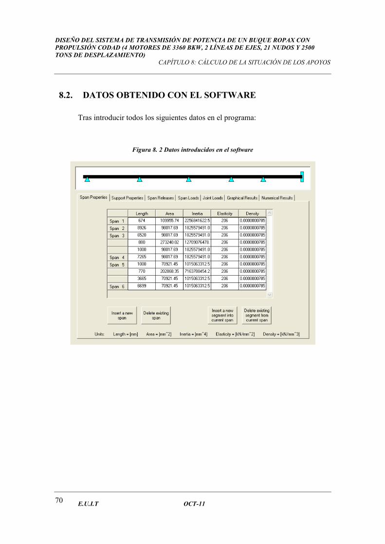
DISEÑO DEL SISTEMA DE TRANSMISIÓN DE POTENCIA DE UN BUQUE ROPAX CON PROPULSIÓN CODAD (4 MOTORES DE 3360 BKW, 2 LÍNEAS DE EJES, 21 NUDOS Y 2500 TONS DE DESPLAZAMIENTO)
CAPÍTULO 8: CÁLCULO DE LA SITUACIÓN DE LOS APOYOS
E.U.I.T OCT-11 70
8.2. DATOS OBTENIDO CON EL SOFTWARE
Tras introducir todos los siguientes datos en el programa:
Figura 8. 2 Datos introducidos en el software
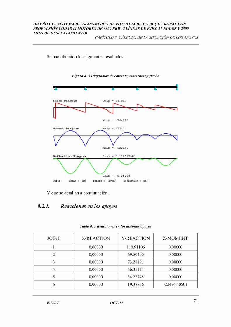
DISEÑO DEL SISTEMA DE TRANSMISIÓN DE POTENCIA DE UN BUQUE ROPAX CON PROPULSIÓN CODAD (4 MOTORES DE 3360 BKW, 2 LÍNEAS DE EJES, 21 NUDOS Y 2500 TONS DE DESPLAZAMIENTO)
CAPÍTULO 8: CÁLCULO DE LA SITUACIÓN DE LOS APOYOS
E.U.I.T OCT-11 71
Se han obtenido los siguientes resultados:
Figura 8. 3 Diagramas de cortante, momentos y flecha
Y que se detallan a continuación.
8.2.1. Reacciones en los apoyos
Tabla 8. 1 Reacciones en los distintos apoyos
JOINT X-REACTION Y-REACTION Z-MOMENT
1 0,00000 110.91106 0,00000
2 0,00000 69.50400 0,00000
3 0,00000 73.28191 0,00000
4 0,00000 46.35127 0,00000
5 0,00000 34.22748 0,00000
6 0,00000 19.38856 -22474.40501
DISEÑO DEL SISTEMA DE TRANSMISIÓN DE POTENCIA DE UN BUQUE ROPAX CON PROPULSIÓN CODAD (4 MOTORES DE 3360 BKW, 2 LÍNEAS DE EJES, 21 NUDOS Y 2500 TONS DE DESPLAZAMIENTO)
CAPÍTULO 8: CÁLCULO DE LA SITUACIÓN DE LOS APOYOS
E.U.I.T OCT-11 72
8.2.2. Esfuerzos cortantes máximos y mínimos
Vmax = 34,917 kN
Vmin = -76,818 kN
8.2.3. Momentos máximos y mínimos
Mmax = 27212 kN×mm
Mmin = -52016 kN×mm
8.2.4. Flexión máxima y mínima
La flecha máxima entre dos apoyos consecutivos debe ser, en valor absoluto,
igual o menor a un milímetro en cada tramo.
Dmax = 0,01 mm
Dmin = -0,35 mm
8.3. COMPROBACIÓN POR CÁLCULO DIRECTO CON LOS
DATOS OBTENIDOS
Hay que hallar el límite elástico y comprobar que es inferior al 30% del límite de
elasticidad del material del eje, 330 N/mm2.
2mm/N993,0330 =×
Luego hay que comprobar que el límite elástico sea inferior a 99 N / mm2.
El límite elástico viene dado por:
)dD(
DMf3244axial
−×π
××=σ
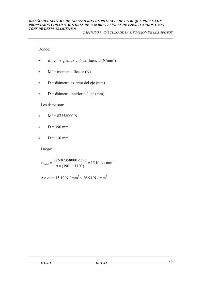
DISEÑO DEL SISTEMA DE TRANSMISIÓN DE POTENCIA DE UN BUQUE ROPAX CON PROPULSIÓN CODAD (4 MOTORES DE 3360 BKW, 2 LÍNEAS DE EJES, 21 NUDOS Y 2500 TONS DE DESPLAZAMIENTO)
CAPÍTULO 8: CÁLCULO DE LA SITUACIÓN DE LOS APOYOS
E.U.I.T OCT-11 73
Donde:
• σaxial = sigma axial ó de fluencia (N/mm2)
• Mf = momento flector (N)
• D = diámetro exterior del eje (mm)
• D = diámetro interior del eje (mm)
Los datos son:
• Mf = 87358000 N
• D = 390 mm
• D = 110 mm
Luego:
2
44axial mm/N10,15)110390(
3908735800032=
−×π
××=σ
Así que: 15,10 N / mm2 < 26,94 N / mm2.

DISEÑO DEL SISTEMA DE TRANSMISIÓN DE POTENCIA DE UN BUQUE ROPAX CON PROPULSIÓN CODAD (4 MOTORES DE 3360 BKW, 2 LÍNEAS DE EJES, 21 NUDOS Y 2500 TONS DE DESPLAZAMIENTO)
CAPÍTULO 9: ELECCION DE LOS APOYOS Y SELLOS DE BOCINA
E.U.I.T OCT-11 75
CAPÍTULO 9. ELECCIÓN DE LOS APOYOS Y
SELLOS DE BOCINA
9.1. APOYOS
Debido a la gran longitud que tienen los ejes de transmisión de potencia, es muy
importante que éstos mantengan su alineación y geometría de diseño. Ésta se consigue
intercalando uno ó varios apoyos entre el primer punto de apoyo, que será el más
cercano a la hélice, y el último, que será la unión del eje con la caja de engranajes.
Estos soportes deben facilitar la transmisión de potencia, reduciendo al máximo
las pérdidas por fricción entre el cojinete y el eje.
Dependiendo de la situación del apoyo se puede diferenciar entre:
• Apoyo del arbotante: es el más cercano a la hélice.
• Apoyos del tubo de bocina: estarán ubicados dentro del tubo de bocina.
• Apoyos intermedios: situados dentro del casco del buque.
Es importante que el material:
• tenga un coeficiente de rozamiento reducido.
• sea un buen transmisor del calor para que no se produzca una acumulación
excesiva de calor, dañando o perjudicando el ajuste creado.
• tenga una cierta dureza para evitar que se deforme por la carga que actúa
sobre él.
DISEÑO DEL SISTEMA DE TRANSMISIÓN DE POTENCIA DE UN BUQUE ROPAX CON PROPULSIÓN CODAD (4 MOTORES DE 3360 BKW, 2 LÍNEAS DE EJES, 21 NUDOS Y 2500 TONS DE DESPLAZAMIENTO)
CAPÍTULO 9: ELECCION DE LOS APOYOS Y SELLOS DE BOCINA
E.U.I.T OCT-11 76
Entre los materiales que cumplen estas propiedades, podemos encontrar:
o Metales blancos: son aleaciones de metales blandos (estaño, plomo, etc..), de bajo punto de fusión , que se funden sobre un soporte metálico al que se adhieren fuertemente y, posteriormente, son mecanizados con grado fino. Generalmente operan con lubricación de aceite.
o Materiales sintéticos rígidos: son derivados plásticos como el tufnol. Son fácilmente mecanizables. Presentan coeficientes de fricción muy bajos, incluso algunos no necesitan lubricación adicional; éstos reciben el nombre de “auto- lubricados”.
o Materiales sintéticos flexibles: son derivados de la goma y caucho; también se vulcanizan sobre un soporte similar a los del metal blando. Esta composición es poco rígida, permitiendo una cierta elasticidad en el soportado que absorbe ruidos y vibraciones. Son especialmente utilizados en arbotantes y bocinas para aprovechar su principal particularidad, como es la lubricación con agua de mar y su inalterabilidad ante ésta.
Principalmente, los apoyos se pueden clasificar, por su forma por constructiva,
en dos grandes grupos: cojinetes de fricción y cojinetes de rodamiento.
Los cojinetes de fricción son unos casquillos de materiales antifricción, sobre los
que se apoyan los ejes para que puedan girar. Pueden ser de una pieza, lo que conlleva a
que su montaje sea axialmente, ó compuesto por dos o más sectores, lo que nos
facilitaría el montaje y desmontaje.
Tienen la ventaja de su marcha tranquila y silenciosa y que pueden construirse
partidos en dos, haciendo posible un montaje y desmontaje radial.
Tienen el inconveniente de que no son indicados en los casos en que se deseen
elevado número de revoluciones, a no ser que la carga que gravita sobre ellos sea
mínima.
En los cojinetes de rodamientos, se intercalan entre el eje y el soporte, una pista
exterior y otra exterior. Entre ellas, se alojan unas bolas o rodillos que sustituyen el
rozamiento de fricción por el de rodadura, que es mucho menor.
DISEÑO DEL SISTEMA DE TRANSMISIÓN DE POTENCIA DE UN BUQUE ROPAX CON PROPULSIÓN CODAD (4 MOTORES DE 3360 BKW, 2 LÍNEAS DE EJES, 21 NUDOS Y 2500 TONS DE DESPLAZAMIENTO)
CAPÍTULO 9: ELECCION DE LOS APOYOS Y SELLOS DE BOCINA
E.U.I.T OCT-11 77
Tienen las ventajas de que el calentamiento y el desgaste son pequeños, admiten
mayores presiones, tanto radiales como axiales, y permiten mayores velocidades.
9.2. CÁLCULO DE LOS COJINETES DE LOS APOYOS
Se usarán cojinetes de metal blanco con base de plomo (SnSb12Cu6Pb) del
fabricante Cedervall & Söner. La fijación del cojinete al tubo de bocina se hará
mediante resina de epoxi. Por ello, habrá que tener en cuenta refrigeración positiva,
orificios de venteo en la parte superior y sensores de temperatura a distancia con alarma,
según la Sociedad de Clasificación Volumen 2, Part 3, Chapter 2 Section 4.16.1.
El eje tendrá un incremento de seis milímetros de diámetro en cada punto de
apoyo, con una longitud igual a la longitud del apoyo más cien milímetros. Este
incremento de diámetro permitiría realizar, si fuese necesario, rectificados de la
superficie de contacto del eje, sin llegar a reducir el diámetro exterior de diseño.
Según la Sociedad de Clasificación Volumen 2, Part 3, Chapter 2 section 4.16.2.,
la longitud de los cojinetes de cola refrigerados por aceite, será aproximadamente dos
veces su diámetro y la presión nominal que soportan no excederá de 0,8 N/mm2. La
longitud de los demás cojinetes de bocina no será inferior a una vez y medio el diámetro
del eje que portan.
Para los cálculos se deben conocer los siguientes datos:
• Diámetro exterior del eje.
• Carga estática en el apoyo.
• Longitud mínima del cojinete.
• Material del cojinete.
• Tipo de refrigeración.
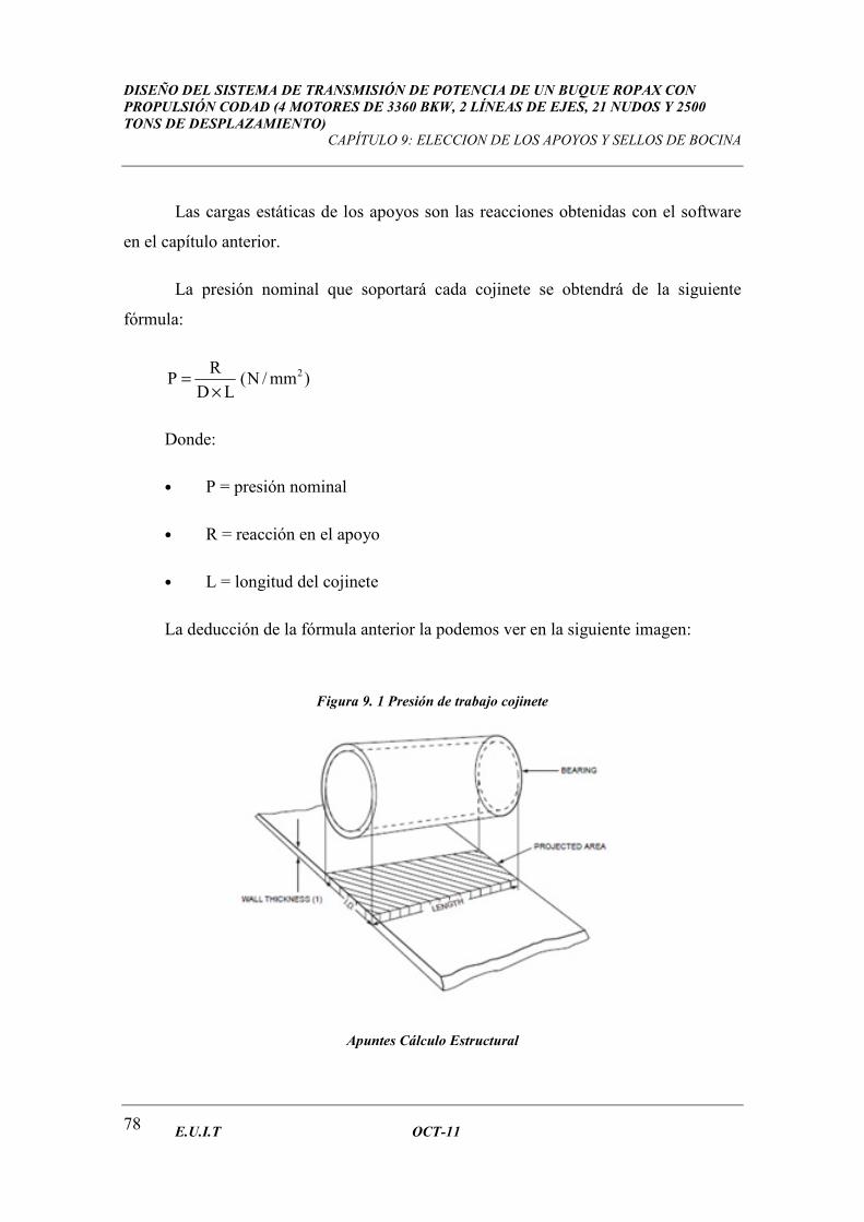
DISEÑO DEL SISTEMA DE TRANSMISIÓN DE POTENCIA DE UN BUQUE ROPAX CON PROPULSIÓN CODAD (4 MOTORES DE 3360 BKW, 2 LÍNEAS DE EJES, 21 NUDOS Y 2500 TONS DE DESPLAZAMIENTO)
CAPÍTULO 9: ELECCION DE LOS APOYOS Y SELLOS DE BOCINA
E.U.I.T OCT-11 78
Las cargas estáticas de los apoyos son las reacciones obtenidas con el software
en el capítulo anterior.
La presión nominal que soportará cada cojinete se obtendrá de la siguiente
fórmula:
)mm/N(LD
RP 2
×=
Donde:
• P = presión nominal
• R = reacción en el apoyo
• L = longitud del cojinete
La deducción de la fórmula anterior la podemos ver en la siguiente imagen:
Figura 9. 1 Presión de trabajo cojinete
Apuntes Cálculo Estructural
DISEÑO DEL SISTEMA DE TRANSMISIÓN DE POTENCIA DE UN BUQUE ROPAX CON PROPULSIÓN CODAD (4 MOTORES DE 3360 BKW, 2 LÍNEAS DE EJES, 21 NUDOS Y 2500 TONS DE DESPLAZAMIENTO)
CAPÍTULO 9: ELECCION DE LOS APOYOS Y SELLOS DE BOCINA
E.U.I.T OCT-11 79
9.2.1. Cojinete del primer apoyo (popa del tubo de bocina)
Datos:
• Diámetro exterior del eje: 390 mm
• Carga estática en el apoyo: 110,91106 kN ⇒ 110911 N según datos
obtenidos del software de cálculo.
La longitud mínima, por Sociedad de Clasificación, viene dada por:
)mm(D2L ×= ⇒ mm7803902L =×=
Teniendo en cuenta que el cojinete del arbotante es el que más desgaste puede
tener por el peso de la hélice, se ha redimensionado hasta 800 mm.
Luego la presión nominal del primer apoyo será:
2mm/N36,0,0800390
110911P =
×=
Se ha seleccionado el apoyo Size 31-40 (de longitud 800 mm) del catálogo
Cedervall sterntube bearings que se muestra en el anexo.
9.2.2. Cojinete del segundo apoyo
Datos:
• Diámetro exterior del eje: 370 mm
• Carga estática en el apoyo: 69,504 kN ⇒ 69504 N según datos obtenidos
del software de cálculo.
DISEÑO DEL SISTEMA DE TRANSMISIÓN DE POTENCIA DE UN BUQUE ROPAX CON PROPULSIÓN CODAD (4 MOTORES DE 3360 BKW, 2 LÍNEAS DE EJES, 21 NUDOS Y 2500 TONS DE DESPLAZAMIENTO)
CAPÍTULO 9: ELECCION DE LOS APOYOS Y SELLOS DE BOCINA
E.U.I.T OCT-11 80
La longitud mínima por Sociedad de Clasificación es:
)mm(D5,1L ×= ⇒ mm5553705,1L =×=
Se ha redimensionado a 600 mm.
Luego la presión nominal del segundo apoyo será:
2mm/N31,0600370
69504P =
×=
Se ha seleccionado el apoyo Size 31-40 (de longitud 600 mm) del catálogo
Cedervall sterntube bearings que se muestra en el anexo.
9.2.3. Cojinete del tercer apoyo
Datos:
• Diámetro exterior del eje: 370 mm
• Carga estática en el apoyo: 73,28191 kN ⇒ 73281 N según datos
obtenidos del software de cálculo.
La longitud mínima por Sociedad de Clasificación es:
)mm(D5,1L ×= ⇒ mm5553705,1L =×=
Se ha redimensionado a 600 mm.
Luego la presión nominal del tercer apoyo será:
2mm/N33,0600370
73281P =
×=
DISEÑO DEL SISTEMA DE TRANSMISIÓN DE POTENCIA DE UN BUQUE ROPAX CON PROPULSIÓN CODAD (4 MOTORES DE 3360 BKW, 2 LÍNEAS DE EJES, 21 NUDOS Y 2500 TONS DE DESPLAZAMIENTO)
CAPÍTULO 9: ELECCION DE LOS APOYOS Y SELLOS DE BOCINA
E.U.I.T OCT-11 81
Se ha seleccionado el apoyo Size 31-40 (de longitud 600 mm) del catálogo
Cedervall sterntube bearings que se muestra en el anexo.
9.2.4. Cojinete del cuarto apoyo (proa del tubo de bocina)
Datos:
• Diámetro exterior del eje: 370 mm
• Carga estática en el apoyo: 46,35127 kN ⇒ 46351 N según datos
obtenidos del software de cálculo.
La longitud mínima por Sociedad de Clasificación es:
)mm(D5,1L ×= ⇒ mm5553705,1L =×=
Se ha redimensionado a 600 mm
Luego la presión nominal del cuarto apoyo será:
2mm/N21,0600370
46351P =
×=
Se ha seleccionado el apoyo Size 31-40 (de longitud 600 mm) del catálogo
Cedervall sterntube bearings que se muestra en el anexo.
9.2.5. Cojinete del apoyo intermedio (cámara de máquinas)
Datos:
• Diámetro exterior del eje: 320 mm
• Carga estática en el apoyo: 34,22748 kN ⇒ 34227 N según datos
obtenidos del software de cálculo.
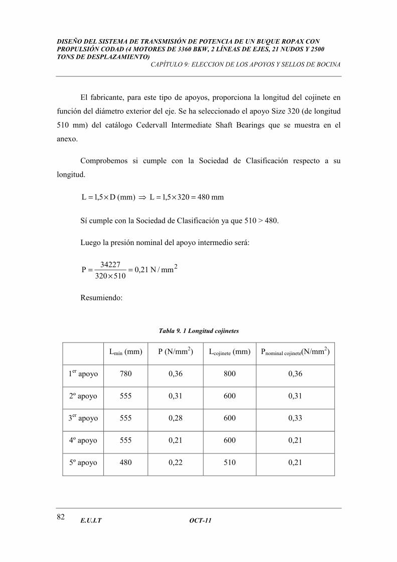
DISEÑO DEL SISTEMA DE TRANSMISIÓN DE POTENCIA DE UN BUQUE ROPAX CON PROPULSIÓN CODAD (4 MOTORES DE 3360 BKW, 2 LÍNEAS DE EJES, 21 NUDOS Y 2500 TONS DE DESPLAZAMIENTO)
CAPÍTULO 9: ELECCION DE LOS APOYOS Y SELLOS DE BOCINA
E.U.I.T OCT-11 82
El fabricante, para este tipo de apoyos, proporciona la longitud del cojinete en
función del diámetro exterior del eje. Se ha seleccionado el apoyo Size 320 (de longitud
510 mm) del catálogo Cedervall Intermediate Shaft Bearings que se muestra en el
anexo.
Comprobemos si cumple con la Sociedad de Clasificación respecto a su
longitud.
)mm(D5,1L ×= ⇒ mm4803205,1L =×=
Sí cumple con la Sociedad de Clasificación ya que 510 > 480.
Luego la presión nominal del apoyo intermedio será:
2mm/N21,0510320
34227P =
×=
Resumiendo:
Tabla 9. 1 Longitud cojinetes
Lmín (mm) P (N/mm2) Lcojinete (mm) Pnominal cojinete(N/mm2)
1er apoyo 780 0,36 800 0,36
2º apoyo 555 0,31 600 0,31
3er apoyo 555 0,28 600 0,33
4º apoyo 555 0,21 600 0,21
5º apoyo 480 0,22 510 0,21
DISEÑO DEL SISTEMA DE TRANSMISIÓN DE POTENCIA DE UN BUQUE ROPAX CON PROPULSIÓN CODAD (4 MOTORES DE 3360 BKW, 2 LÍNEAS DE EJES, 21 NUDOS Y 2500 TONS DE DESPLAZAMIENTO)
CAPÍTULO 9: ELECCION DE LOS APOYOS Y SELLOS DE BOCINA
E.U.I.T OCT-11 83
Donde:
• Lmín = longitud mínima exigida por la Sociedad de Clasificación.
• P = presión obtenida según fórmula.
• Lcojinete = longitud del cojinete seleccionado.
• Pnominal cojinete = presión nominal del cojinete seleccionado.
9.3. SELLOS DE BOCINA
Los sellos de bocina serán dos: uno a popa y otro a proa del tubo de bocina.
Ambos serán del fabricante Cedervall & Söner.
El sello de popa será Size 16, para diámetro exterior de eje de 378 mm a 396
mm, como se muestra en el catálogo del anexo.
El sello de proa será Size 15, para diámetro exterior de eje de 359 mm a 377
mm, como se muestra en el catálogo del anexo.
9.4. PASAMAMPARO ESTANCO DEL EJE
El pasamamparo será size 320 para diámetro exterior de eje de 301 mm a 320
mm como se muestra en el catálogo anexo.
Será suministrado por el fabricante Blohm + Voss Industries.

DISEÑO DEL SISTEMA DE TRANSMISIÓN DE POTENCIA DE UN BUQUE ROPAX CON PROPULSIÓN CODAD (4 MOTORES DE 3360 BKW, 2 LÍNEAS DE EJES, 21 NUDOS Y 2500 TONS DE DESPLAZAMIENTO)
BIBLIOGRAFÍA
E.U.I.T OCT-11 85
BIBLIOGRAFÍA
Apuntes de la asignatura de Cálculo Estructural
Rules and Regulations for the Classification of Naval Ships Lloyd’s Register, Edición
2002
Norma ISO 4032 tercera edición 1999-03-15,Hexagon nuts, style1-Product grade A and
B
Norma ISO 4014 tercera edición 1999-09-01,Hexagon head bolts-Product grade A and
B
Norma ISO 7089 segunda edición 2000-06-01,Plain washers-Normal series-Product
grade A.
Norma ISO 898-1 tercera edición 1999-08-01,Mechanical properties of fasteners of
carbon steel and alloy steel.
Manual imprescindible de Autocad 2000, Antonio Manuel Reyes Rodríguez, primera
edición, septiembre 1999.
Guía práctica Autocad 2010, Fernando Montaño La Cruz EDICIONES ANAYA
MULTIMEDIA, 2010.
SOFTWARE UTILIZADOS
Autocad 2007
Microsoft Office 2003
DT Beam versión 1.0
PÁGINAS WEB CONSULTADAS
http://www.answers.com/topic/combined-diesel-and-diesel

DISEÑO DEL SISTEMA DE TRANSMISIÓN DE POTENCIA DE UN BUQUE ROPAX CON PROPULSIÓN CODAD (4 MOTORES DE 3360 BKW, 2 LÍNEAS DE EJES, 21 NUDOS Y 2500 TONS DE DESPLAZAMIENTO)
BIBLIOGRAFÍA
E.U.I.T OCT-11 86
http://www.vulkan.com/fileadmin/product_db/assets/RATO%20RTechnical%20Data.p
df
http://www.ingenierosnanales.com/docurevista/PAG.%2051-61.pdf
http://www.skf.com/iec_documents/OK_1.pdf
http://www.mandieselturbo.com/article_004544.html
http://translate.google.es
http://www.rae.es/rae.html
http://imistorage.blob.core.windows.net/imidocs/2100p008%20sterntube%20bearings.p
df
http://www.cedervall.com/images/pdf/produkter/CEDN.pdf

DISEÑO DEL SISTEMA DE TRANSMISIÓN DE POTENCIA DE UN BUQUE ROPAX CON PROPULSIÓN CODAD (4 MOTORES DE 3360 BKW, 2 LÍNEAS DE EJES, 21 NUDOS Y 2500 TONS DE DESPLAZAMIENTO)
ANEXO
E.U.I.T OCT-11 87
Anexo
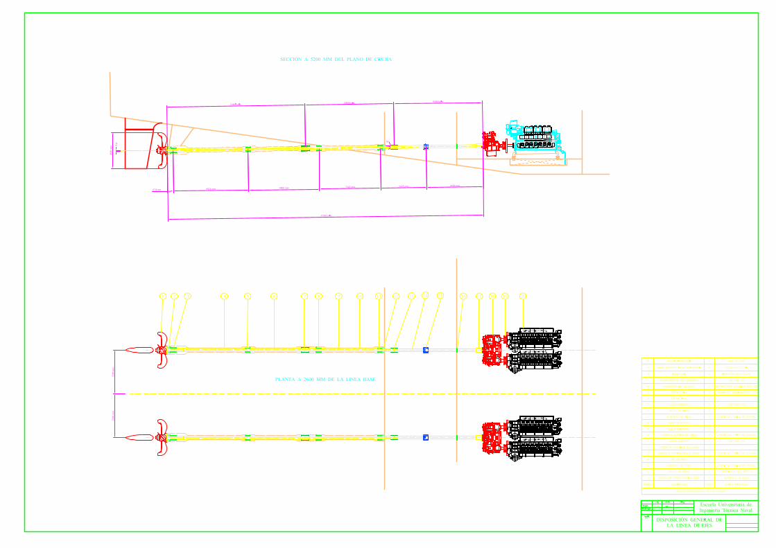
OK shaft couplings
Contents3 The clever connection4 The OK coupling explained6 OKC 100 - 1907 OKC 200 - 4008 OKC 410 - 4908 OKC 500 - 5209 OKC 530 - 100010 OKF 100 - 30011 OKF 310 - 70012 OKCS 178 - 36013 OKTC 245 - 79014 Tailor-made OK couplings15 Power transmission capacity15 Safety factors16 Shafts16 Conversion tables17 Hollow shafts for OKC17 Hollow shafts for OKCS and OKF18 Modular equipment for mounting and dismounting20 Oil20 Approved by leading classification societies21 Locating device for outer sleeve21 Mounting arrangements for OKC couplings22 The Supergrip bolt cuts down on downtime
2
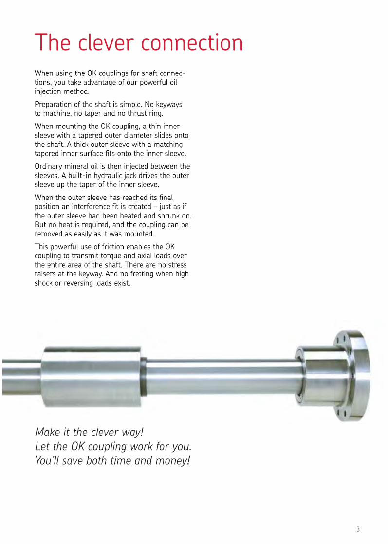
When using the OK couplings for shaft connec-tions, you take advantage of our powerful oilinjection method.
Preparation of the shaft is simple. No keyways to machine, no taper and no thrust ring.
When mounting the OK coupling, a thin innersleeve with a tapered outer diameter slides ontothe shaft. A thick outer sleeve with a matchingtapered inner surface fits onto the inner sleeve.
Ordinary mineral oil is then injected between thesleeves. A built-in hydraulic jack drives the outersleeve up the taper of the inner sleeve.
When the outer sleeve has reached its finalposition an interference fit is created – just as ifthe outer sleeve had been heated and shrunk on.But no heat is required, and the coupling can beremoved as easily as it was mounted.
This powerful use of friction enables the OKcoupling to transmit torque and axial loads overthe entire area of the shaft. There are no stressraisers at the keyway. And no fretting when highshock or reversing loads exist.
Make it the clever way!Let the OK coupling work for you.You’ll save both time and money!
3
The clever connection
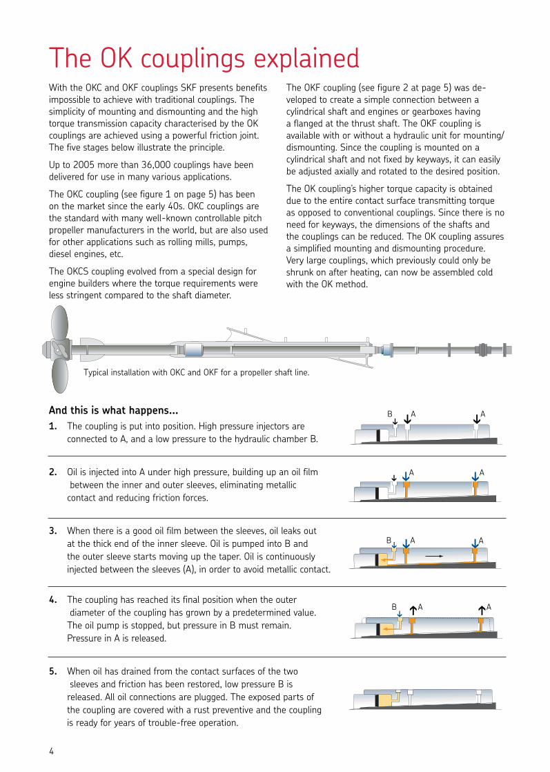
The OK couplings explainedWith the OKC and OKF couplings SKF presents benefitsimpossible to achieve with traditional couplings. Thesimplicity of mounting and dismounting and the hightorque transmission capacity characterised by the OKcouplings are achieved using a powerful friction joint.The five stages below illustrate the principle.
Up to 2005 more than 36,000 couplings have beendelivered for use in many various applications.
The OKC coupling (see figure 1 on page 5) has been on the market since the early 40s. OKC couplings arethe standard with many well-known controllable pitchpropeller manufacturers in the world, but are also usedfor other applications such as rolling mills, pumps,diesel engines, etc.
The OKCS coupling evolved from a special design forengine builders where the torque requirements wereless stringent compared to the shaft diameter.
The OKF coupling (see figure 2 at page 5) was de-veloped to create a simple connection between acylindrical shaft and engines or gearboxes having a flanged at the thrust shaft. The OKF coupling isavailable with or without a hydraulic unit for mounting/dismounting. Since the coupling is mounted on acylindrical shaft and not fixed by keyways, it can easilybe adjusted axially and rotated to the desired position.
The OK coupling’s higher torque capacity is obtaineddue to the entire contact surface transmitting torqueas opposed to conventional couplings. Since there is noneed for keyways, the dimensions of the shafts and the couplings can be reduced. The OK coupling assuresa simplified mounting and dismounting procedure.Very large couplings, which previously could only beshrunk on after heating, can now be assembled coldwith the OK method.
4
Typical installation with OKC and OKF for a propeller shaft line.
And this is what happens...1. The coupling is put into position. High pressure injectors are
connected to A, and a low pressure to the hydraulic chamber B.
2. Oil is injected into A under high pressure, building up an oil filmbetween the inner and outer sleeves, eliminating metallic
contact and reducing friction forces.
3. When there is a good oil film between the sleeves, oil leaks outat the thick end of the inner sleeve. Oil is pumped into B and the outer sleeve starts moving up the taper. Oil is continuouslyinjected between the sleeves (A), in order to avoid metallic contact.
4. The coupling has reached its final position when the outerdiameter of the coupling has grown by a predetermined value.
The oil pump is stopped, but pressure in B must remain. Pressure in A is released.
5. When oil has drained from the contact surfaces of the twosleeves and friction has been restored, low pressure B is
released. All oil connections are plugged. The exposed parts of the coupling are covered with a rust preventive and the coupling is ready for years of trouble-free operation.
A
A
A A
AA
A
AB
B
B
➔➔ ➔
➔➔
➔
➔ ➔
➔➔
➔➔
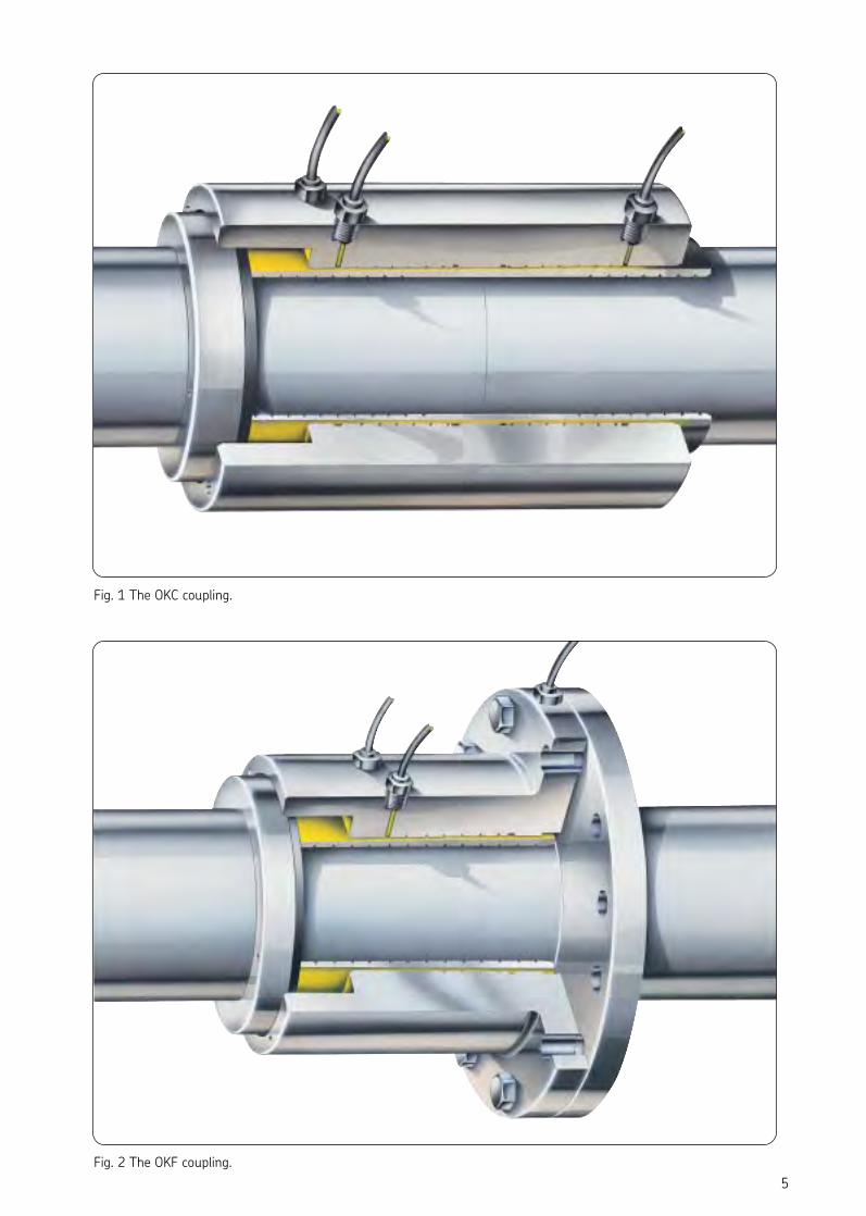
Fig. 1 The OKC coupling.
Fig. 2 The OKF coupling.5
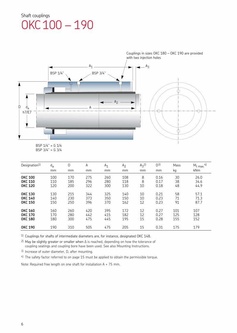
Designation1) da D A A1 A2 A32) D3) Mass Mt max.4)
mm mm mm mm mm mm mm kg kNm
OKC 100 100 170 275 260 108 8 0.16 30 26.0OKC 110 110 185 296 280 118 8 0.17 38 34.6OKC 120 120 200 322 300 130 10 0.18 48 44.9
OKC 130 130 215 344 325 140 10 0.21 58 57.1OKC 140 140 230 373 350 150 10 0.23 71 71.3OKC 150 150 250 396 370 162 12 0.23 91 87.7
OKC 160 160 260 420 395 172 12 0.27 101 107OKC 170 170 280 442 415 182 12 0.27 125 128OKC 180 180 300 475 445 195 15 0.28 155 152
OKC 190 190 310 505 475 205 15 0.31 175 179
Shaft couplings
OKC100 – 190
Couplings in sizes OKC 180 – OKC 190 are providedwith two injection holes
BSP 1/4” = G 1/4BSP 3/4” = G 3/4
BSP 3/4”BSP 1/4”
6
D dah7/E7
A1
A2A
A3
1) Couplings for shafts of intermediate diameters are, for instance, designated OKC 148.2) May be slightly greater or smaller when D is reached, depending on how the tolerance of
coupling seatings and coupling bore have been used. See also Mounting Instructions.3) Increase of outer diameter, D, after mounting.4) The safety factor referred to on page 15 must be applied to obtain the permissible torque.
Note: Required free length on one shaft for installation A + 75 mm.
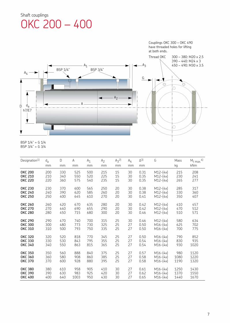
Designation1) da D A A1 A2 A32) A4 D3) G Mass Mt max.4)
mm mm mm mm mm mm mm mm kg kNm
OKC 200 200 330 525 500 215 15 30 0.31 M12-(4x) 215 208OKC 210 210 340 550 520 225 15 30 0.35 M12-(4x) 230 241OKC 220 220 360 575 540 235 15 30 0.35 M12-(4x) 265 277
OKC 230 230 370 600 565 250 20 30 0.38 M12-(4x) 285 317OKC 240 240 390 620 585 260 20 30 0.38 M12-(4x) 330 360OKC 250 250 400 645 610 270 20 30 0.41 M12-(4x) 350 407
OKC 260 260 420 670 635 280 20 30 0.42 M12-(4x) 410 457OKC 270 270 440 690 655 290 20 30 0.42 M12-(4x) 470 512OKC 280 280 450 715 680 300 20 30 0.46 M12-(4x) 510 571
OKC 290 290 470 740 700 315 25 30 0.46 M12-(4x) 580 634OKC 300 300 480 773 730 325 25 27 0.50 M16-(4x) 625 702OKC 310 310 500 793 750 335 25 27 0.50 M16-(4x) 700 775
OKC 320 320 520 818 770 345 25 27 0.50 M16-(4x) 790 852OKC 330 330 530 843 795 355 25 27 0.54 M16-(4x) 830 935OKC 340 340 550 863 815 365 25 27 0.54 M16-(4x) 930 1020
OKC 350 350 560 888 840 375 25 27 0.57 M16-(4x) 980 1120OKC 360 360 580 908 860 385 25 27 0.58 M16-(4x) 1080 1220OKC 370 370 600 928 880 395 25 27 0.58 M16-(4x) 1190 1320
OKC 380 380 610 958 905 410 30 27 0.61 M16-(4x) 1250 1430OKC 390 390 630 983 925 420 30 27 0.62 M16-(4x) 1370 1550OKC 400 400 640 1003 950 430 30 27 0.65 M16-(4x) 1440 1670
Shaft couplings
OKC 200 – 400
BSP 1/4” = G 1/4BSP 3/4” = G 3/4
BSP 3/4”BSP 1/4”
7
Couplings OKC 300 – OKC 490have threaded holes for liftingat both ends.
Thread OKC 300 – 380: M20 x 2.5390 – 440: M24 x 3450 – 490: M30 x 3.5
D dah7/E7
A1
A4
A2
A
A3
G
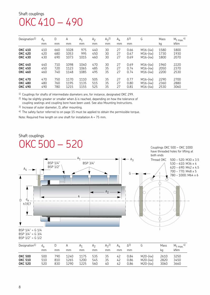
Designation1) da D A A1 A2 A32) A4 D3) G Mass Mt max.4)
mm mm mm mm mm mm mm mm kg kNm
OKC 500 500 790 1240 1175 535 35 42 0.84 M20-(4x) 2610 3250OKC 510 510 810 1265 1200 545 35 42 0.86 M20-(4x) 2820 3450OKC 520 520 830 1290 1225 560 40 42 0.86 M20-(4x) 3060 3660
8
Designation1) da D A A1 A2 A32) A4 D3) G Mass Mt max.4)
mm mm mm mm mm mm mm mm kg kNm
OKC 410 410 660 1028 975 440 30 27 0.66 M16-(4x) 1580 1800OKC 420 420 680 1053 995 450 30 27 0.67 M16-(4x) 1730 1930OKC 430 430 690 1073 1015 460 30 27 0.69 M16-(4x) 1800 2070
OKC 440 440 710 1098 1040 470 30 27 0.69 M16-(4x) 1960 2220OKC 450 450 720 1123 1065 485 35 27 0.74 M16-(4x) 2050 2370OKC 460 460 740 1148 1085 495 35 27 0.74 M16-(4x) 2200 2530
OKC 470 470 750 1170 1110 505 35 27 0.77 M16-(4x) 2290 2700OKC 480 480 760 1195 1135 515 35 27 0.80 M16-(4x) 2360 2880OKC 490 490 780 1215 1155 525 35 27 0.81 M16-(4x) 2530 3060
D
BSP 1/4” = G 1/4BSP 3/4” = G 3/4BSP 1/2” = G 1/2
BSP 1/4” BSP 1/2”
BSP 3/4” A3
A4
A2A
A1
G
dah7/E7
1) Couplings for shafts of intermediate diameters are, for instance, designated OKC 299.2) May be slightly greater or smaller when D is reached, depending on how the tolerance of
coupling seatings and coupling bore have been used. See also Mounting Instructions.3) Increase of outer diameter, D, after mounting.4) The safety factor referred to on page 15 must be applied to obtain the permissible torque.
Note: Required free length on one shaft for installation A + 75 mm.
Couplings OKC 500 – OKC 1000have threaded holes for lifting at both endsThread OKC 500 – 520: M30 x 3.5
530 – 610: M36 x 4620 – 690: M42 x 4.5700 – 770: M48 x 5780 – 1000: M64 x 6
Shaft couplings
OKC410 – 490
Shaft couplings
OKC500 – 520
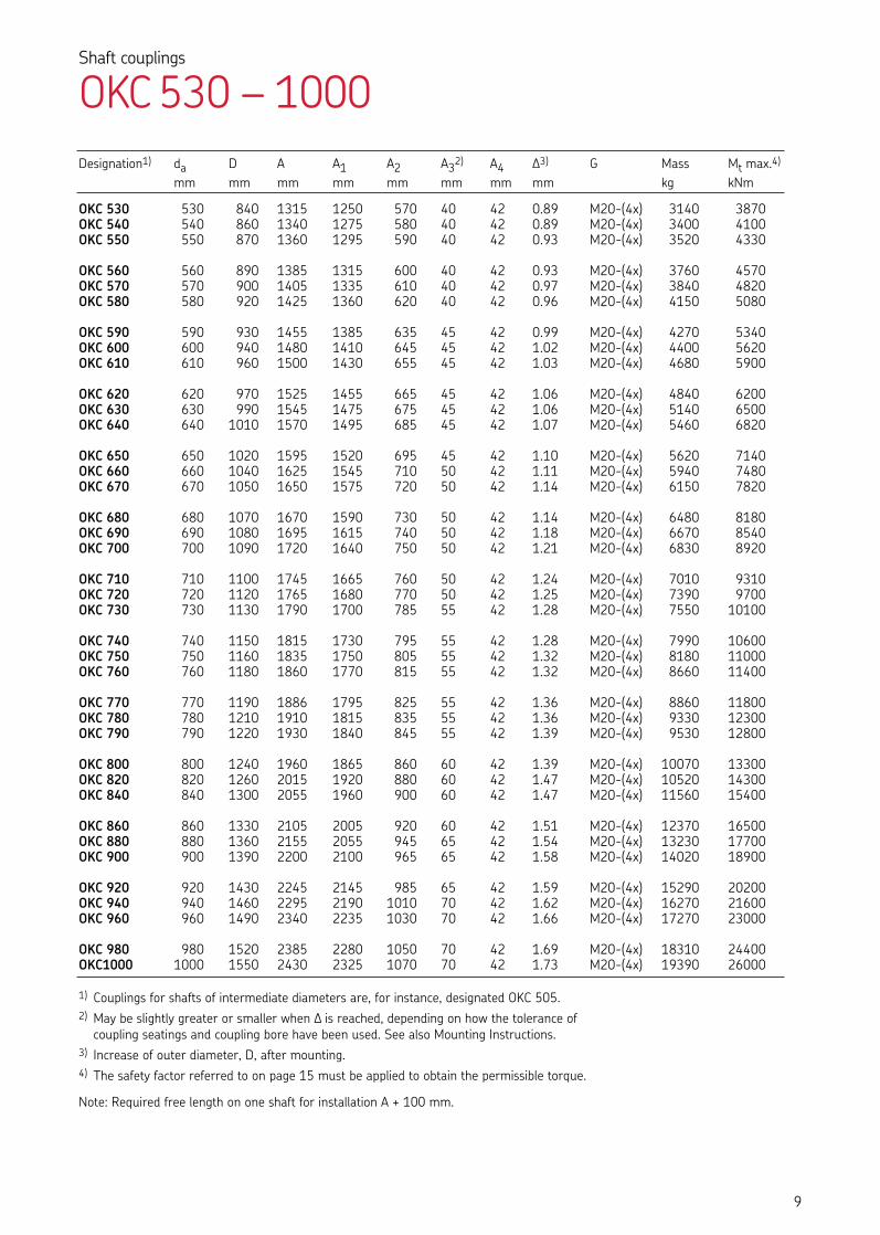
Designation1) da D A A1 A2 A32) A4 D3) G Mass Mt max.4)
mm mm mm mm mm mm mm mm kg kNm
OKC 530 530 840 1315 1250 570 40 42 0.89 M20-(4x) 3140 3870OKC 540 540 860 1340 1275 580 40 42 0.89 M20-(4x) 3400 4100OKC 550 550 870 1360 1295 590 40 42 0.93 M20-(4x) 3520 4330
OKC 560 560 890 1385 1315 600 40 42 0.93 M20-(4x) 3760 4570OKC 570 570 900 1405 1335 610 40 42 0.97 M20-(4x) 3840 4820OKC 580 580 920 1425 1360 620 40 42 0.96 M20-(4x) 4150 5080
OKC 590 590 930 1455 1385 635 45 42 0.99 M20-(4x) 4270 5340OKC 600 600 940 1480 1410 645 45 42 1.02 M20-(4x) 4400 5620OKC 610 610 960 1500 1430 655 45 42 1.03 M20-(4x) 4680 5900
OKC 620 620 970 1525 1455 665 45 42 1.06 M20-(4x) 4840 6200OKC 630 630 990 1545 1475 675 45 42 1.06 M20-(4x) 5140 6500OKC 640 640 1010 1570 1495 685 45 42 1.07 M20-(4x) 5460 6820
OKC 650 650 1020 1595 1520 695 45 42 1.10 M20-(4x) 5620 7140OKC 660 660 1040 1625 1545 710 50 42 1.11 M20-(4x) 5940 7480OKC 670 670 1050 1650 1575 720 50 42 1.14 M20-(4x) 6150 7820
OKC 680 680 1070 1670 1590 730 50 42 1.14 M20-(4x) 6480 8180OKC 690 690 1080 1695 1615 740 50 42 1.18 M20-(4x) 6670 8540OKC 700 700 1090 1720 1640 750 50 42 1.21 M20-(4x) 6830 8920
OKC 710 710 1100 1745 1665 760 50 42 1.24 M20-(4x) 7010 9310OKC 720 720 1120 1765 1680 770 50 42 1.25 M20-(4x) 7390 9700OKC 730 730 1130 1790 1700 785 55 42 1.28 M20-(4x) 7550 10100
OKC 740 740 1150 1815 1730 795 55 42 1.28 M20-(4x) 7990 10600OKC 750 750 1160 1835 1750 805 55 42 1.32 M20-(4x) 8180 11000OKC 760 760 1180 1860 1770 815 55 42 1.32 M20-(4x) 8660 11400
OKC 770 770 1190 1886 1795 825 55 42 1.36 M20-(4x) 8860 11800OKC 780 780 1210 1910 1815 835 55 42 1.36 M20-(4x) 9330 12300OKC 790 790 1220 1930 1840 845 55 42 1.39 M20-(4x) 9530 12800
OKC 800 800 1240 1960 1865 860 60 42 1.39 M20-(4x) 10070 13300OKC 820 820 1260 2015 1920 880 60 42 1.47 M20-(4x) 10520 14300OKC 840 840 1300 2055 1960 900 60 42 1.47 M20-(4x) 11560 15400
OKC 860 860 1330 2105 2005 920 60 42 1.51 M20-(4x) 12370 16500OKC 880 880 1360 2155 2055 945 65 42 1.54 M20-(4x) 13230 17700OKC 900 900 1390 2200 2100 965 65 42 1.58 M20-(4x) 14020 18900
OKC 920 920 1430 2245 2145 985 65 42 1.59 M20-(4x) 15290 20200OKC 940 940 1460 2295 2190 1010 70 42 1.62 M20-(4x) 16270 21600OKC 960 960 1490 2340 2235 1030 70 42 1.66 M20-(4x) 17270 23000
OKC 980 980 1520 2385 2280 1050 70 42 1.69 M20-(4x) 18310 24400OKC1000 1000 1550 2430 2325 1070 70 42 1.73 M20-(4x) 19390 26000
9
1) Couplings for shafts of intermediate diameters are, for instance, designated OKC 505.2) May be slightly greater or smaller when D is reached, depending on how the tolerance of
coupling seatings and coupling bore have been used. See also Mounting Instructions.3) Increase of outer diameter, D, after mounting.4) The safety factor referred to on page 15 must be applied to obtain the permissible torque.
Note: Required free length on one shaft for installation A + 100 mm.
Shaft couplings
OKC530 – 1000
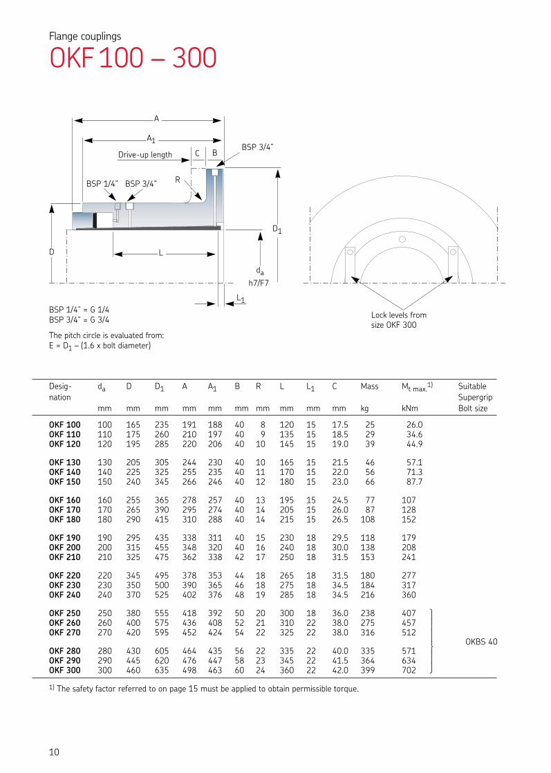
Desig- da D D1 A A1 B R L L1 C Mass Mt max.1) Suitablenation Supergrip
mm mm mm mm mm mm mm mm mm mm kg kNm Bolt size
OKF 100 100 165 235 191 188 40 8 120 15 17.5 25 26.0OKF 110 110 175 260 210 197 40 9 135 15 18.5 29 34.6OKF 120 120 195 285 220 206 40 10 145 15 19.0 39 44.9
OKF 130 130 205 305 244 230 40 10 165 15 21.5 46 57.1OKF 140 140 225 325 255 235 40 11 170 15 22.0 56 71.3OKF 150 150 240 345 266 246 40 12 180 15 23.0 66 87.7
OKF 160 160 255 365 278 257 40 13 195 15 24.5 77 107OKF 170 170 265 390 295 274 40 14 205 15 26.0 87 128OKF 180 180 290 415 310 288 40 14 215 15 26.5 108 152
OKF 190 190 295 435 338 311 40 15 230 18 29.5 118 179OKF 200 200 315 455 348 320 40 16 240 18 30.0 138 208OKF 210 210 325 475 362 338 42 17 250 18 31.5 153 241
OKF 220 220 345 495 378 353 44 18 265 18 31.5 180 277OKF 230 230 350 500 390 365 46 18 275 18 34.5 184 317OKF 240 240 370 525 402 376 48 19 285 18 34.5 216 360
OKF 250 250 380 555 418 392 50 20 300 18 36.0 238 407OKF 260 260 400 575 436 408 52 21 310 22 38.0 275 457OKF 270 270 420 595 452 424 54 22 325 22 38.0 316 512
OKBS 40OKF 280 280 430 605 464 435 56 22 335 22 40.0 335 571OKF 290 290 445 620 476 447 58 23 345 22 41.5 364 634OKF 300 300 460 635 498 463 60 24 360 22 42.0 399 702
1) The safety factor referred to on page 15 must be applied to obtain permissible torque.
Drive-up length
The pitch circle is evaluated from:E = D1 – (1.6 x bolt diameter)
Lock levels fromsize OKF 300
L1
dah7/F7
D
C B
R
L
D1
BSP 1/4” BSP 3/4”
BSP 3/4”
BSP 1/4” = G 1/4BSP 3/4” = G 3/4
A1
A
10
Flange couplings
OKF100 – 300
rssfsc
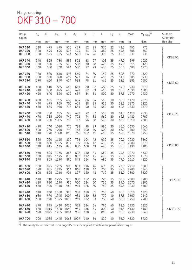
Desig- da D D1 A A1 B R L L1 C Mass Mt max.1) Suitablenation Supergrip
mm mm mm mm mm mm mm mm mm mm kg kNm Bolt size
OKF 310 310 475 675 510 479 62 25 370 22 43.5 451 775OKF 320 320 495 695 526 494 64 26 380 25 44.5 508 852OKF 330 330 505 705 544 512 66 26 395 25 46.5 537 935
OKBS 50OKF 340 340 525 730 555 522 68 27 405 25 47.0 599 1020OKF 350 350 530 735 572 538 70 28 420 25 49.0 615 1120OKF 360 360 550 760 584 550 72 29 430 25 50.0 680 1220
OKF 370 370 570 810 595 560 74 30 440 25 50.5 770 1320OKF 380 380 580 820 612 577 76 30 455 25 51.5 805 1430OKF 390 390 600 840 624 588 78 31 465 25 52.5 885 1550
OKBS 60OKF 400 400 610 855 648 611 80 32 480 25 54.0 930 1670OKF 410 410 630 875 660 627 82 33 490 30 55.5 1030 1800OKF 420 420 640 890 672 639 84 34 500 30 57.5 1070 1930
OKF 430 430 655 935 688 654 86 34 515 30 58.0 1170 2070OKF 440 440 675 955 700 665 88 35 525 30 58.5 1270 2220OKF 450 450 685 970 716 681 90 36 540 30 60.5 1330 2370
OKF 460 460 700 985 728 692 92 37 550 30 61.5 1410 2530 OKBS 70OKF 470 470 715 1000 740 703 94 38 560 30 62.5 1480 2700OKF 480 480 720 1005 758 717 96 38 570 30 65.0 1510 2880
OKF 490 490 740 1030 770 728 98 39 580 30 66.0 1630 3060OKF 500 500 750 1040 790 748 100 40 600 30 67.0 1700 3250OKF 510 510 770 1090 810 766 102 41 610 35 69.5 1870 3450
OKF 520 520 790 1115 820 776 104 42 620 35 70.0 2020 3660OKF 530 530 800 1125 834 789 106 42 630 35 72.0 2080 3870OKF 540 540 815 1145 845 800 108 43 640 35 73.5 2190 4100 OKBS 80
OKF 550 550 825 1155 868 822 110 44 660 35 74.5 2270 4330OKF 560 560 845 1175 878 832 112 45 670 35 75.0 2420 4570OKF 570 570 855 1190 890 843 114 46 680 35 77.0 2510 4820
OKF 580 580 875 1235 900 853 116 46 690 35 77.0 2710 5080OKF 590 590 885 1245 914 866 118 47 700 35 79.0 2780 5340OKF 600 600 895 1260 926 877 120 48 710 35 81.0 2860 5620
OKF 610 610 910 1275 938 888 122 49 720 35 82.0 2880 5900 OKBS 90OKF 620 620 920 1290 950 900 124 50 730 35 84.0 3070 6200OKF 630 630 940 1310 962 911 126 50 740 35 84.5 3230 6500
OKF 640 640 960 1330 990 938 128 51 760 40 85.5 3510 6820OKF 650 650 970 1345 1004 951 130 52 770 40 87.5 3600 7140OKF 660 660 990 1395 1018 961 132 53 780 40 88.0 3750 7480
OKF 670 670 995 1410 1030 973 134 54 790 40 91.0 3930 7820OKF 680 680 1015 1420 1042 984 136 54 800 40 91.5 4130 8180 OKBS 100OKF 690 690 1025 1435 1054 996 138 55 810 40 93.5 4230 8540
OKF 700 700 1035 1445 1068 1009 140 56 820 40 96.0 4330 8920
1) The safety factor referred to on page 15 must be applied to obtain the permissible torque.
11
Flange couplings
OKF310 – 700
rssfsssc
rsssfsssc
rsssfsssc
rsfsssc
rssfsssc
rssfsc
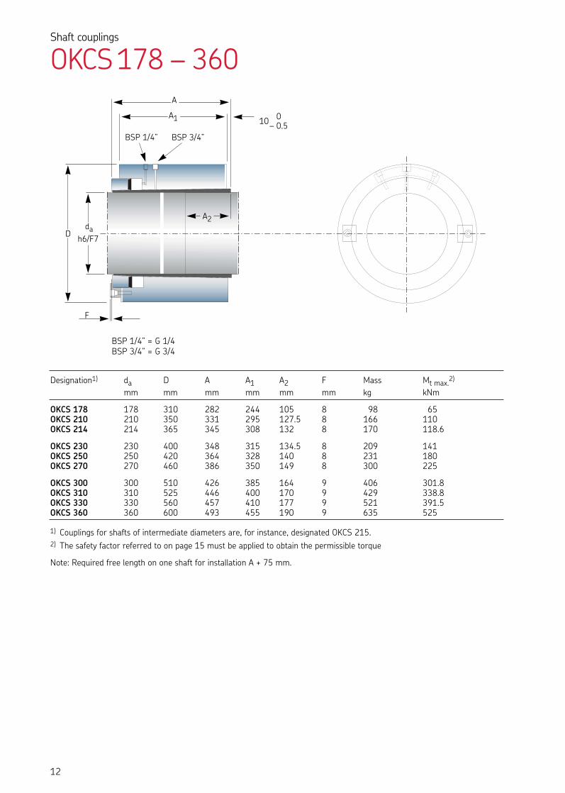
– 010– 0.5
12
Designation1) da D A A1 A2 F Mass Mt max.2)
mm mm mm mm mm mm kg kNm
OKCS 178 178 310 282 244 105 8 98 65OKCS 210 210 350 331 295 127.5 8 166 110OKCS 214 214 365 345 308 132 8 170 118.6
OKCS 230 230 400 348 315 134.5 8 209 141OKCS 250 250 420 364 328 140 8 231 180OKCS 270 270 460 386 350 149 8 300 225
OKCS 300 300 510 426 385 164 9 406 301.8OKCS 310 310 525 446 400 170 9 429 338.8OKCS 330 330 560 457 410 177 9 521 391.5OKCS 360 360 600 493 455 190 9 635 525
BSP 1/4” = G 1/4BSP 3/4” = G 3/4
BSP 3/4” BSP 1/4”
D
F
A1
A2
A
dah6/F7
1) Couplings for shafts of intermediate diameters are, for instance, designated OKCS 215.2) The safety factor referred to on page 15 must be applied to obtain the permissible torque
Note: Required free length on one shaft for installation A + 75 mm.
Shaft couplings
OKCS178 – 360
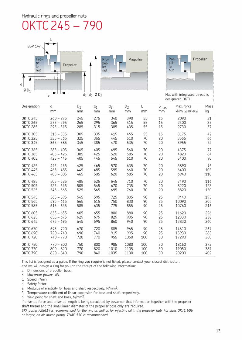
This list is designed as a guide. If the ring you require is not listed, please contact your closest distributor,and we will design a ring for you on the receipt of the following information:a. Dimensions of propeller boss.b. Maximum power, kW.c. Speed, r/min.d. Safety factor.e. Modulus of elasticity for boss and shaft respectively, N/mm2.f. Temperature coefficient of linear expansion for boss and shaft respectively.g. Yield point for shaft and boss, N/mm2.If drive-up force and drive-up length is being calculated by customer that information together with the propellershaft thread and the small inner diameter of the propeller boss only are required.SKF pump 728619 is recommended for the ring as well as for injecting oil in the propeller hub. For sizes OKTC 505 or larger, an air driven pump, THAP 150 is recommended.
Designation d D1 d1 d2 D2 L Smax. Max. force Massmm mm mm mm mm mm mm kNm (at 70 MPa) kg
OKTC 245 260 – 275 245 275 340 390 55 15 2090 31OKTC 265 275 – 295 265 295 365 415 55 15 2400 35OKTC 285 295 – 315 285 315 385 435 55 15 2730 37
OKTC 305 315 – 335 305 335 415 465 55 15 3175 42OKTC 325 335 – 365 325 365 445 510 70 20 3555 66OKTC 345 365 – 385 345 385 470 535 70 20 3955 72
OKTC 365 385 – 405 365 405 495 560 70 20 4375 77OKTC 385 405 – 425 385 425 520 585 70 20 4820 84OKTC 405 425 – 445 405 445 545 610 70 20 5400 90
OKTC 425 445 – 465 425 465 570 635 70 20 5890 96OKTC 445 465 – 485 445 485 595 660 70 20 6400 103OKTC 465 485 – 505 465 505 620 685 70 20 6940 110
OKTC 485 505 – 525 485 525 645 710 70 20 7490 116OKTC 505 525 – 545 505 545 670 735 70 20 8220 123OKTC 525 545 – 565 525 565 695 760 70 20 8820 130
OKTC 545 565 – 595 545 595 725 805 90 25 9440 195OKTC 565 595 – 615 565 615 750 830 90 25 10090 205OKTC 585 615 – 635 585 635 775 855 90 25 10760 216
OKTC 605 635 – 655 605 655 800 880 90 25 11620 226OKTC 625 655 – 675 625 675 825 905 90 25 12330 238OKTC 645 675 – 695 645 695 860 940 90 25 13830 260
OKTC 670 695 – 720 670 720 885 965 90 25 14610 267OKTC 690 720 – 740 690 740 915 995 90 25 15930 285OKTC 720 740 – 770 720 770 955 1050 100 30 17290 360
OKTC 750 770 – 800 750 800 985 1080 100 30 18160 372OKTC 770 800 – 820 770 820 1010 1105 100 30 19050 387OKTC 790 820 – 840 790 840 1035 1130 100 30 20200 402
Nut with integrated thread isdesignated OKTH.
Ø D1Ø D2d2d1S
d
L
BSP 1/4”
Propeller Propeller Pro-pel-lernut
Pro-pel-lernut
Pro-pel-lernut
13
Propeller
Hydraulic rings and propeller nuts
OKTC245 – 790
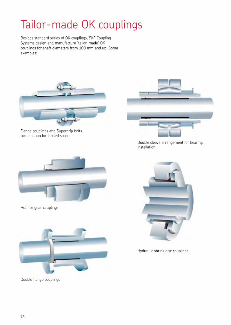
Besides standard series of OK couplings, SKF CouplingSystems design and manufacture ‘‘tailor-made’’ OKcouplings for shaft diameters from 100 mm and up. Someexamples:
Tailor-made OK couplings
14
Flange couplings and Supergrip boltscombination for limited space
Hub for gear couplings
Hydraulic shrink disc couplings
Double sleeve arrangement for bearinginstallation
Double flange couplings
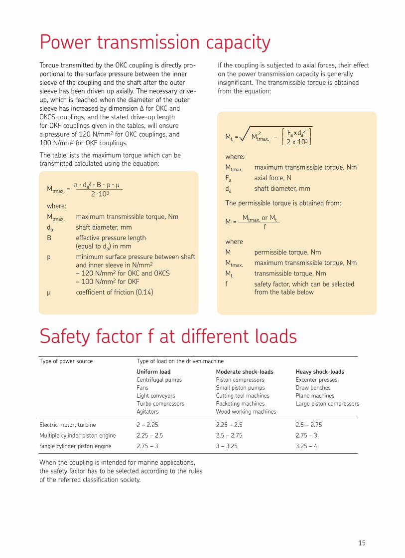
2 Fax da2
Mt =P Mtmax. – 2 x 10³
where:Mtmax. maximum transmissible torque, NmFa axial force, Nda shaft diameter, mm
The permissible torque is obtained from:
Mtmax. or MtM =f
whereM permissible torque, NmMtmax. maximum transmissible torque, NmMt transmissible torque, Nmf safety factor, which can be selected
from the table below
If the coupling is subjected to axial forces, their effecton the power transmission capacity is generallyinsignificant. The transmissible torque is obtained from the equation:
Torque transmitted by the OKC coupling is directly pro-portional to the surface pressure between the innersleeve of the coupling and the shaft after the outersleeve has been driven up axially. The necessary drive-up, which is reached when the diameter of the outersleeve has increased by dimension D for OKC andOKCS couplings, and the stated drive-up length for OKF couplings given in the tables, will ensure a pressure of 120 N/mm2 for OKC couplings, and 100 N/mm2 for OKF couplings.
The table lists the maximum torque which can betransmitted calculated using the equation:
p . da2 . B . p . µMtmax. =2 .103
where:Mtmax. maximum transmissible torque, Nmda shaft diameter, mmB effective pressure length
(equal to da) in mmp minimum surface pressure between shaft
and inner sleeve in N/mm2
– 120 N/mm2 for OKC and OKCS– 100 N/mm2 for OKF
µ coefficient of friction (0.14)
Power transmission capacity
Safety factor f at different loadsType of power source Type of load on the driven machine
Uniform load Moderate shock-loads Heavy shock-loadsCentrifugal pumps Piston compressors Excenter pressesFans Small piston pumps Draw benchesLight conveyors Cutting tool machines Plane machinesTurbo compressors Packeting machines Large piston compressorsAgitators Wood working machines
Electric motor, turbine 2 – 2.25 2.25 – 2.5 2.5 – 2.75
Multiple cylinder piston engine 2.25 – 2.5 2.5 – 2.75 2.75 – 3
Single cylinder piston engine 2.75 – 3 3 – 3.25 3.25 – 4
When the coupling is intended for marine applications,the safety factor has to be selected according to the rulesof the referred classification society.
15
tav
ysb
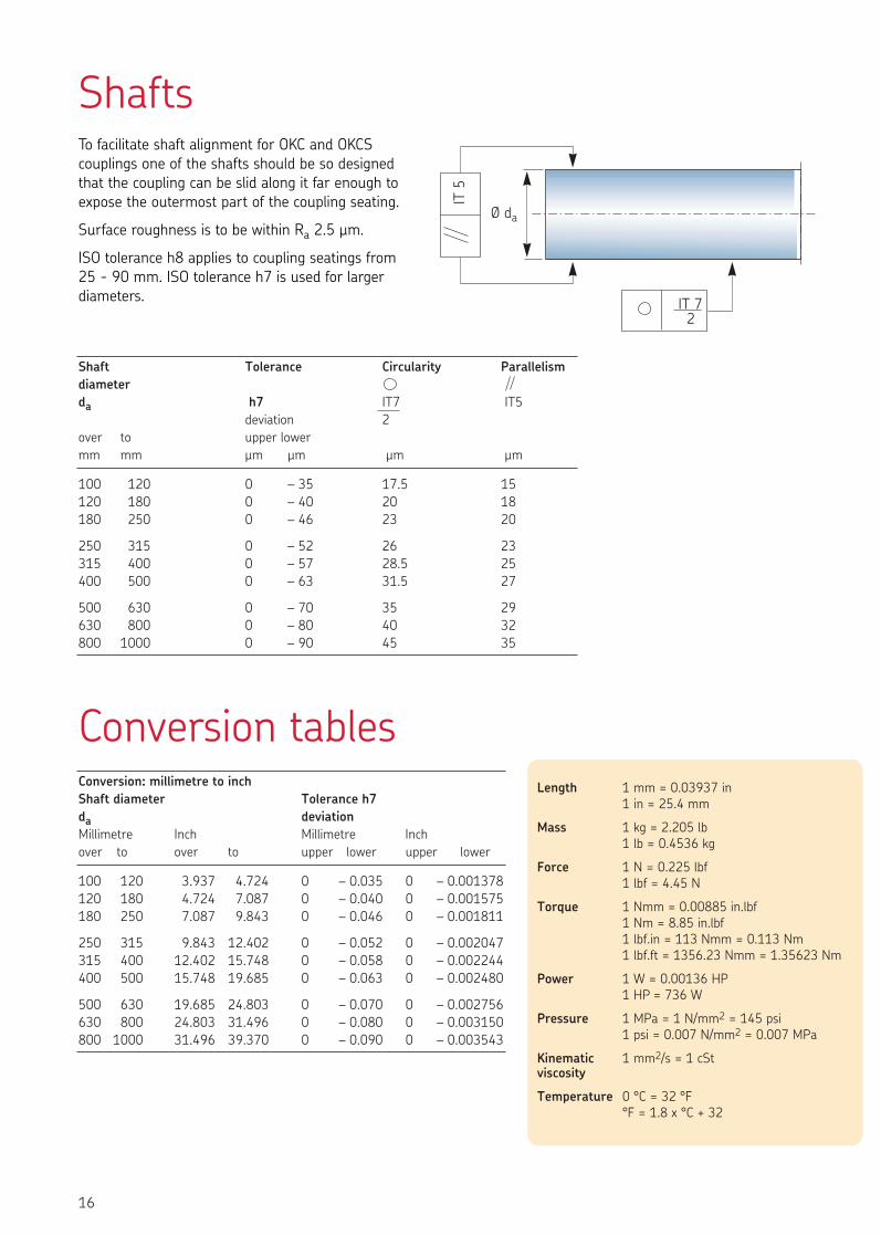
IT 72
Ø da
IT 5
Shafts
Conversion tables
To facilitate shaft alignment for OKC and OKCScouplings one of the shafts should be so designed that the coupling can be slid along it far enough toexpose the outermost part of the coupling seating.
Surface roughness is to be within Ra 2.5 µm.
ISO tolerance h8 applies to coupling seatings from25 - 90 mm. ISO tolerance h7 is used for largerdiameters.
Length 1 mm = 0.03937 in1 in = 25.4 mm
Mass 1 kg = 2.205 lb1 lb = 0.4536 kg
Force 1 N = 0.225 lbf1 lbf = 4.45 N
Torque 1 Nmm = 0.00885 in.lbf1 Nm = 8.85 in.lbf1 lbf.in = 113 Nmm = 0.113 Nm1 lbf.ft = 1356.23 Nmm = 1.35623 Nm
Power 1 W = 0.00136 HP1 HP = 736 W
Pressure 1 MPa = 1 N/mm2 = 145 psi1 psi = 0.007 N/mm2 = 0.007 MPa
Kinematic 1 mm2/s = 1 cStviscosity
Temperature 0 °C = 32 °F°F = 1.8 x °C + 32
Conversion: millimetre to inchShaft diameter Tolerance h7da deviationMillimetre Inch Millimetre Inchover to over to upper lower upper lower
100 120 3.937 4.724 0 – 0.035 0 – 0.001378120 180 4.724 7.087 0 – 0.040 0 – 0.001575180 250 7.087 9.843 0 – 0.046 0 – 0.001811
250 315 9.843 12.402 0 – 0.052 0 – 0.002047315 400 12.402 15.748 0 – 0.058 0 – 0.002244400 500 15.748 19.685 0 – 0.063 0 – 0.002480
500 630 19.685 24.803 0 – 0.070 0 – 0.002756630 800 24.803 31.496 0 – 0.080 0 – 0.003150800 1000 31.496 39.370 0 – 0.090 0 – 0.003543
Shaft Tolerance Circularity Parallelismdiameterda h7 IT7 IT5
deviation 2over to upper lowermm mm µm µm µm µm
100 120 0 – 35 17.5 15120 180 0 – 40 20 18180 250 0 – 46 23 20
250 315 0 – 52 26 23315 400 0 – 57 28.5 25400 500 0 – 63 31.5 27
500 630 0 – 70 35 29630 800 0 – 80 40 32800 1000 0 – 90 45 35
16
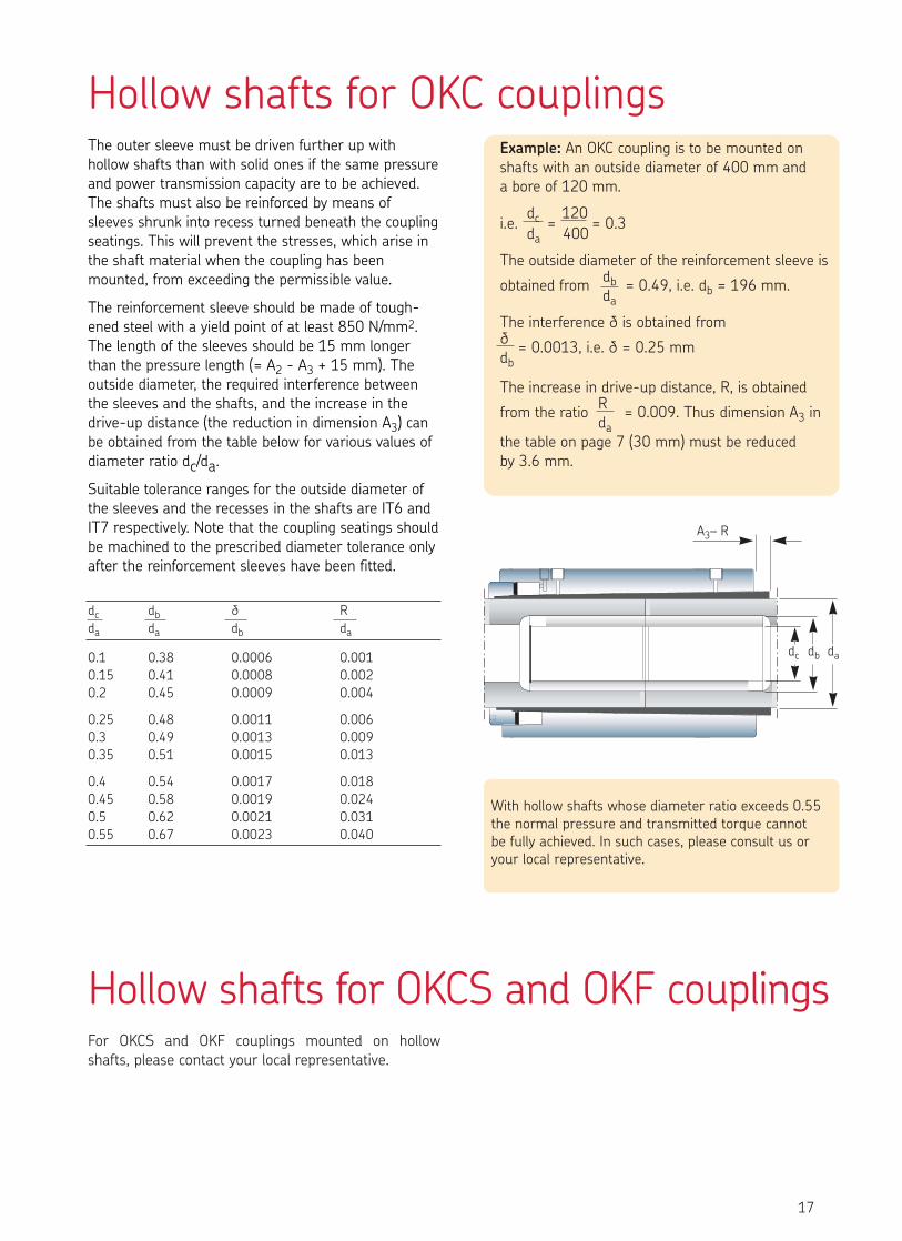
Hollow shafts for OKC couplings
Hollow shafts for OKCS and OKF couplings
The outer sleeve must be driven further up withhollow shafts than with solid ones if the same pressureand power transmission capacity are to be achieved.The shafts must also be reinforced by means ofsleeves shrunk into recess turned beneath the couplingseatings. This will prevent the stresses, which arise inthe shaft material when the coupling has beenmounted, from exceeding the permissible value.
The reinforcement sleeve should be made of tough-ened steel with a yield point of at least 850 N/mm2.The length of the sleeves should be 15 mm longerthan the pressure length (= A2 - A3 + 15 mm). Theoutside diameter, the required interference betweenthe sleeves and the shafts, and the increase in thedrive-up distance (the reduction in dimension A3) canbe obtained from the table below for various values ofdiameter ratio dc/da.
Suitable tolerance ranges for the outside diameter ofthe sleeves and the recesses in the shafts are IT6 andIT7 respectively. Note that the coupling seatings shouldbe machined to the prescribed diameter tolerance onlyafter the reinforcement sleeves have been fitted.
Example: An OKC coupling is to be mounted on shafts with an outside diameter of 400 mm and a bore of 120 mm.
dc 120i.e. = = 0.3
da 400
The outside diameter of the reinforcement sleeve isdbobtained from = 0.49, i.e. db = 196 mm.da
The interference d is obtained fromd = 0.0013, i.e. d = 0.25 mmdb
The increase in drive-up distance, R, is obtainedRfrom the ratio = 0.009. Thus dimension A3 in da
the table on page 7 (30 mm) must be reduced by 3.6 mm.
With hollow shafts whose diameter ratio exceeds 0.55the normal pressure and transmitted torque cannotbe fully achieved. In such cases, please consult us oryour local representative.
dc db d Rda da db da
0.1 0.38 0.0006 0.0010.15 0.41 0.0008 0.0020.2 0.45 0.0009 0.004
0.25 0.48 0.0011 0.0060.3 0.49 0.0013 0.0090.35 0.51 0.0015 0.013
0.4 0.54 0.0017 0.0180.45 0.58 0.0019 0.0240.5 0.62 0.0021 0.0310.55 0.67 0.0023 0.040
For OKCS and OKF couplings mounted on hollowshafts, please contact your local representative.
17
A3– R
dc db da
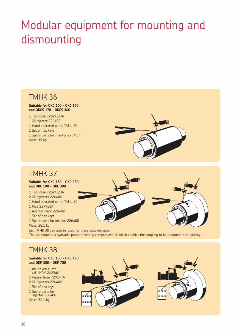
TMHK 38 Suitable for OKC 180 - OKC 490and OKF 300 - OKF 700
1 Air-driven pump set THAP 030/SET
1 Return hose 729147A2 Oil injectors 2264001 Set of hex keys1 Spare parts for
injector 226400Mass: 32.1 kg
TMHK 37Suitable for OKC 180 - OKC 250and OKF 100 - OKF 300
1 Tool case 728245/3A2 Oil injectors 2264001 Hand operated pump TMJL 501 Pipe 227958A1 Adapter block 2264021 Set of hex keys1 Spare parts for injector 226400Mass: 28.1 kg Set TMHK 38 can also be used for these coupling sizes.The set contains a hydraulic pump driven by compressed air which enables the coupling to be mounted more quickly.
TMHK 36Suitable for OKC 100 - OKC 170and OKCS 178 - OKCS 360
1 Tool case 728245/3A1 Oil injector 2264001 Hand operated pump TMJL 501 Set of hex keys1 Spare parts for injector 226400Mass: 19 kg
18
Modular equipment for mounting anddismounting
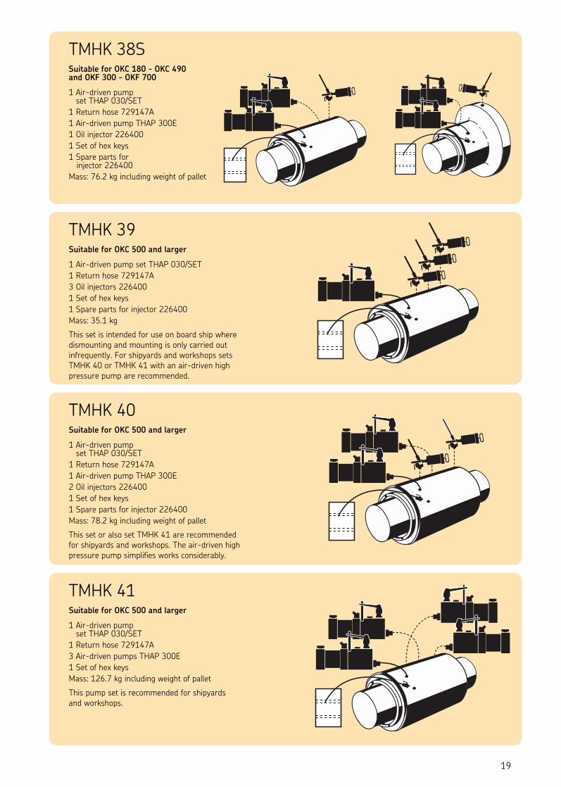
TMHK 41Suitable for OKC 500 and larger
1 Air-driven pumpset THAP 030/SET
1 Return hose 729147A3 Air-driven pumps THAP 300E1 Set of hex keysMass: 126.7 kg including weight of pallet
This pump set is recommended for shipyardsand workshops.
TMHK 38SSuitable for OKC 180 - OKC 490and OKF 300 - OKF 700
1 Air-driven pump set THAP 030/SET
1 Return hose 729147A1 Air-driven pump THAP 300E1 Oil injector 2264001 Set of hex keys1 Spare parts for
injector 226400Mass: 76.2 kg including weight of pallet
TMHK 39Suitable for OKC 500 and larger
1 Air-driven pump set THAP 030/SET1 Return hose 729147A3 Oil injectors 2264001 Set of hex keys1 Spare parts for injector 226400Mass: 35.1 kg
This set is intended for use on board ship wheredismounting and mounting is only carried outinfrequently. For shipyards and workshops setsTMHK 40 or TMHK 41 with an air-driven highpressure pump are recommended.
TMHK 40Suitable for OKC 500 and larger
1 Air-driven pump set THAP 030/SET
1 Return hose 729147A1 Air-driven pump THAP 300E2 Oil injectors 2264001 Set of hex keys1 Spare parts for injector 226400Mass: 78.2 kg including weight of pallet
This set or also set TMHK 41 are recommendedfor shipyards and workshops. The air-driven high pressure pump simplifies works considerably.
19

20
Approved by leading classification societiesConnecting rigid shafts with OK couplings is a time-saving solution that has been usen on land and at seafor more than fifty years. The couplings are well knownall over the world for their high quality, creative designand operational safety.
In the production line each step is carefully controlledand the finished couplings are subjected to a rigid finalinspection regarding sizes and steel quality beforedelivery. The couplings are also approved by all majorclassification societies, for example Det Norske Veritas.
OilThe mineral motor oil to be used for the hydraulicpump and the injectors should have a viscosity of 300 mm2/s (300 cSt) at the temperature of thecoupling. This viscosity will generally be obtained with sufficient accuracy if the oil is chosen accordingto the table below.
Temperature Viscosityrange
0 – 8 °C mineral motor oil SAE 10 W8 – 18 °C mineral motor oil SAE 20 W18 – 27 °C mineral motor oil SAE 30 W27 – 32 °C mineral motor oil SAE 40 W32 – 38 °C mineral motor oil SAE 50 W
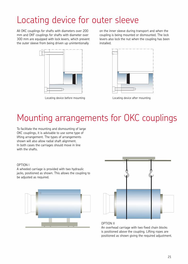
Locating device for outer sleeve
Mounting arrangements for OKC couplings
All OKC couplings for shafts with diameters over 200mm and OKF couplings for shafts with diameter over300 mm are equipped with lock levers, which preventthe outer sleeve from being driven up unintentionally
To facilitate the mounting and dismounting of largeOKC couplings, it is advisable to use some type oflifting arrangement. The types of arrangements shown will also allow radial shaft alignment. In both cases the carriages should move in line with the shafts.
OPTION IIAn overhead carriage with two fixed chain blocks is positioned above the coupling. Lifting ropes arepositioned as shown giving the required adjustment.
OPTION IA wheeled carriage is provided with two hydraulicjacks, positioned as shown. This allows the coupling tobe adjusted as required.
on the inner sleeve during transport and when thecoupling is being mounted or dismounted. The locklevers also lock the nut when the coupling has beeninstalled.
Locating device before mounting Locating device after mounting
21
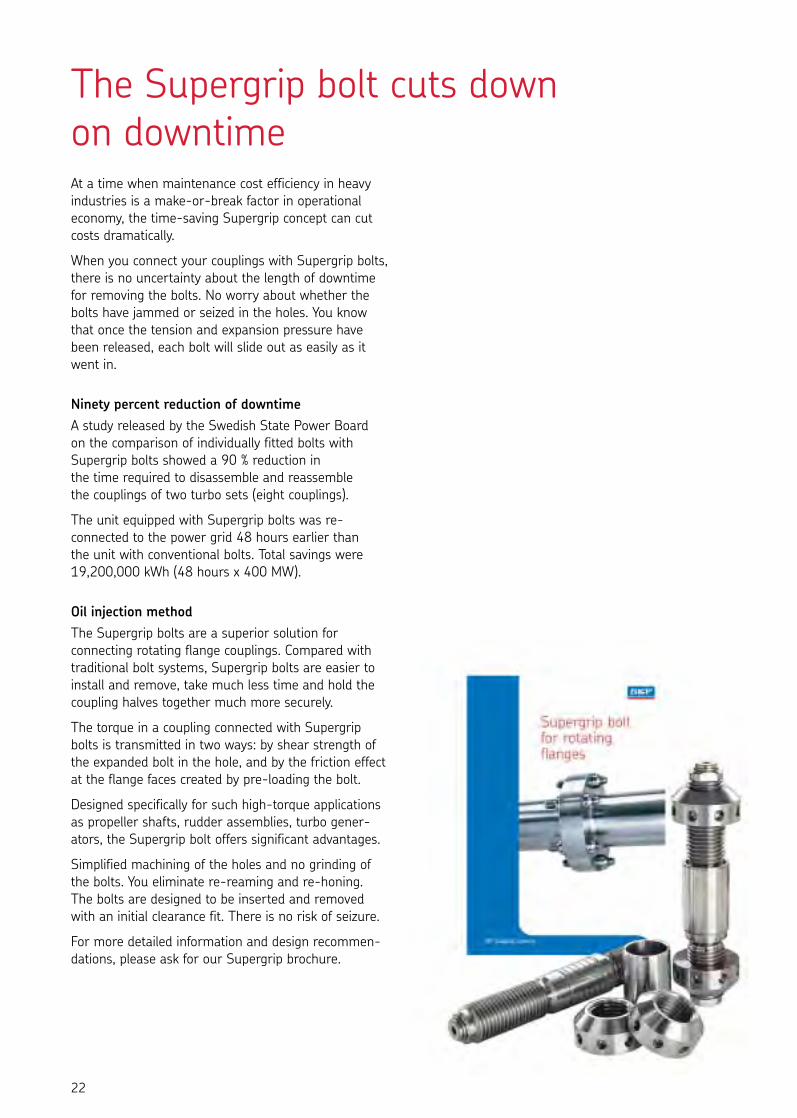
The Supergrip bolt cuts down on downtimeAt a time when maintenance cost efficiency in heavyindustries is a make-or-break factor in operationaleconomy, the time-saving Supergrip concept can cutcosts dramatically.
When you connect your couplings with Supergrip bolts,there is no uncertainty about the length of downtimefor removing the bolts. No worry about whether thebolts have jammed or seized in the holes. You knowthat once the tension and expansion pressure havebeen released, each bolt will slide out as easily as itwent in.
Ninety percent reduction of downtimeA study released by the Swedish State Power Board on the comparison of individually fitted bolts withSupergrip bolts showed a 90 % reduction in the time required to disassemble and reassemble the couplings of two turbo sets (eight couplings).
The unit equipped with Supergrip bolts was re-connected to the power grid 48 hours earlier than the unit with conventional bolts. Total savings were19,200,000 kWh (48 hours x 400 MW).
Oil injection methodThe Supergrip bolts are a superior solution for connecting rotating flange couplings. Compared withtraditional bolt systems, Supergrip bolts are easier toinstall and remove, take much less time and hold thecoupling halves together much more securely.
The torque in a coupling connected with Supergripbolts is transmitted in two ways: by shear strength ofthe expanded bolt in the hole, and by the friction effectat the flange faces created by pre-loading the bolt.
Designed specifically for such high-torque applicationsas propeller shafts, rudder assemblies, turbo gener-ators, the Supergrip bolt offers significant advantages.
Simplified machining of the holes and no grinding ofthe bolts. You eliminate re-reaming and re-honing.The bolts are designed to be inserted and removedwith an initial clearance fit. There is no risk of seizure.
For more detailed information and design recommen-dations, please ask for our Supergrip brochure.
22
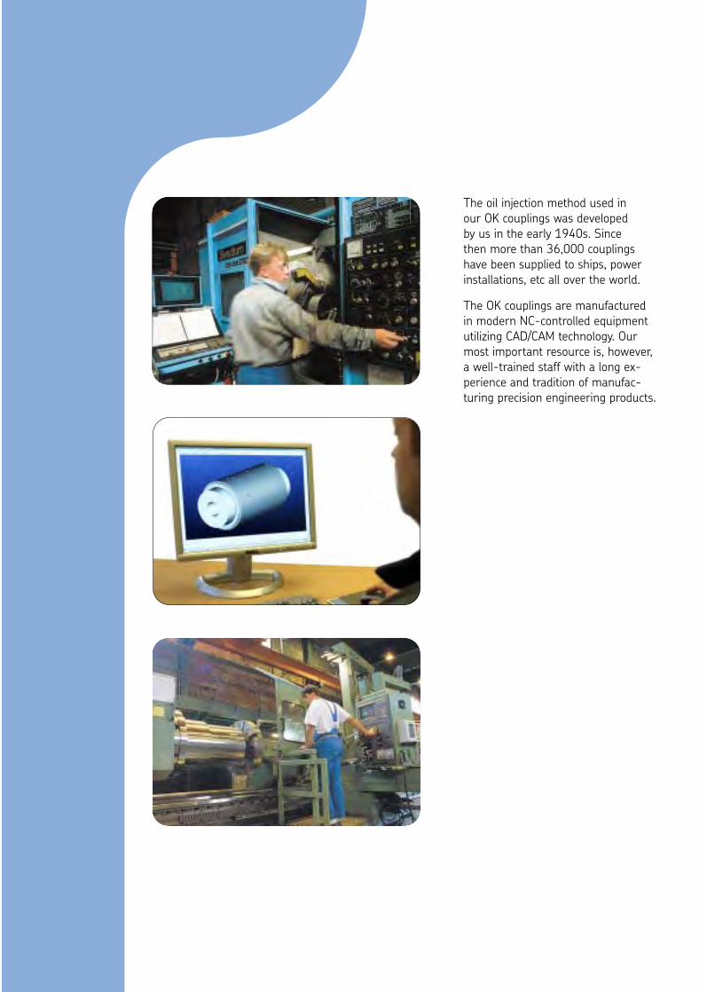
The oil injection method used inour OK couplings was developed by us in the early 1940s. Since then more than 36,000 couplingshave been supplied to ships, powerinstallations, etc all over the world.
The OK couplings are manufacturedin modern NC-controlled equipmentutilizing CAD/CAM technology. Ourmost important resource is, however,a well-trained staff with a long ex-perience and tradition of manufac-turing precision engineering products.

SE-813 82 Hofors, Sweden. Tel: +46 290 284 00. Fax: +46 290 282 70E-mail: [email protected]: www.couplings.skf.com
SKF Coupling Systems AB wasestablished in the early 1940s whenSKF’s Chief Designer, Erland Bratt,invented the SKF oil injection method.As the result of continuous develop-ment, SKF is currently a world leaderin selected market niches.
Our business concept is to develop,produce and supply products basedon the SKF oil injection method.These products significantly reducedowntime and lower maintenancecosts of the capital-intensive equip-ment in which they are used.
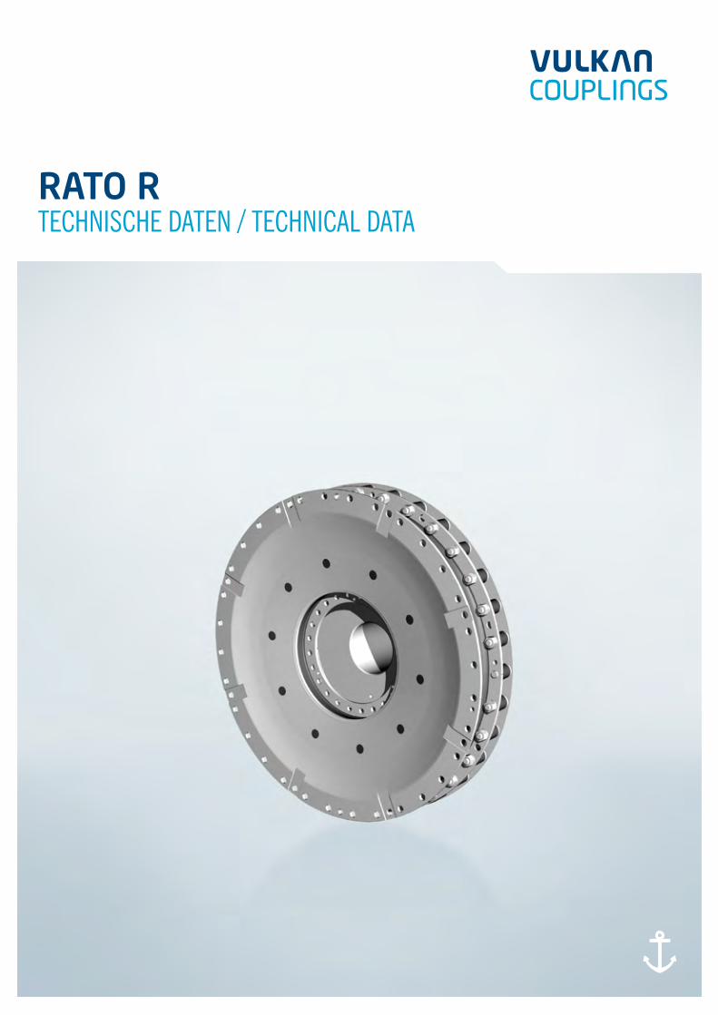
Rato RTechnische DaTen / Technical DaTa
Validity Clause
The present catalogue shall replace all previous editions, any previous printings
shall no longer be valid. Based on new developments, VULKAN reserves the right
to amend and change any details contained in this catalogue respectively. The new
data shall only apply with respect to couplings that were ordered after said amend-
ment or change. It shall be the responsibility of the user to ensure that only the
latest catalogue issue will be used. The respective latest issue can be seen on the
website of VULKAN on www.vulkan.com.
The data contained in this catalogue refer to the technical standard as presently
used by VULKAN with defined conditions according to the explanations. It shall be
the sole responsibility and decision of the system administrator for the drive line to
draw conclusions about the system behaviour.
VULKAN torsional vibration analysis usually only consider the pure mechanical
mass-elastic system. Being a component manufacturer exclusively, VULKAN
assumes no system responsibility with the analysis of the torsional vibration system
(stationary, transiently)! The accuracy of the analysis depends on the exactness of
the used data and the data VULKAN is provided with, respectively.
Any changes due to the technological progress are reserved. For questions or
queries please contact VULKAN.
Status: 01/2011
All duplication, reprinting and translation rights are reserved.
We reserve the right to modify dimensions and constructions without prior notice.
GültiGkeitsklausel
Die vorliegende Broschüre ersetzt alle vorherigen Ausgaben, ältere Drucke verlieren
ihre Gültigkeit. VULKAN ist berechtigt, aufgrund neuerer Entwicklungen die in
dieser Broschüre enthaltenen Daten entsprechend anzupassen und zu verändern.
Die neuen Daten gelten nur für nach der Änderung bestellte Kupplungen. Es liegt
im Verantwortungsbereich des Anwenders dafür zu sorgen, dass ausschließlich
die aktuelle Katalogversion verwendet wird. Der jeweils aktuelle Stand ist auf der
Webseite von VULKAN unter www.vulkan.com jederzeit abrufbar.
Die Angaben in dieser Broschüre beziehen sich auf den technischen Standard
gültig im Hause VULKAN und stehen unter den in den Erläuterungen definierten
Bedingungen. Es liegt allein im Entscheidungs- und Verantwortungsrahmen des
Systemverantwort-lichen für die Antriebslinie, entsprechende Rückschlüsse auf das
Systemverhalten zu ziehen.
VULKAN Drehschwingungsanalysen berücksichtigen in der Regel nur das rein mech-
anische Schwingungsersatzsystem. Als reiner Komponentenhersteller übernimmt
VULKAN mit der Analyse des Drehschwingungssystems (stationär, transient) nicht
die Systemverantwortung! Die Genauigkeit der Analyse hängt von der Genauigkeit
der verwendeten bzw. der VULKAN zur Verfügung gestellten Daten ab.
Änderungen aufgrund des technischen Fortschritts sind vorbehalten. Bei Unklar-
heiten bzw. Rückfragen kontaktieren Sie bitte VULKAN.
Stand 01/2011
Das Recht auf Vervielfältigung, Nachdruck und Übersetzungen behalten wir uns vor.
Maß- und Konstruktionsänderungen vorbehalten.
02 RatO R

inhaltsVeRzeiChniscOnTenTs
GültiGkeitsklausel ValiDiTy clause
03
04
06
02inhaltsVeRzeiChnis cOnTenTs
eiGensChaften und BesChReiBunGcharacTerisTics anD DescripTiOn
liste deR teChnisChen datenlisT Of Technical DaTa
08 aBmessunGen/massentRäGheitsmOmente/massenDimensiOns/mass-mOmenTs Of inerTia/masses
08 RatO R Baureihe 2200 / series 2200
10 RatO R Baureihe 2201 / series 2201
12 RatO R Baureihe 2400 / series 2400
03RatO R
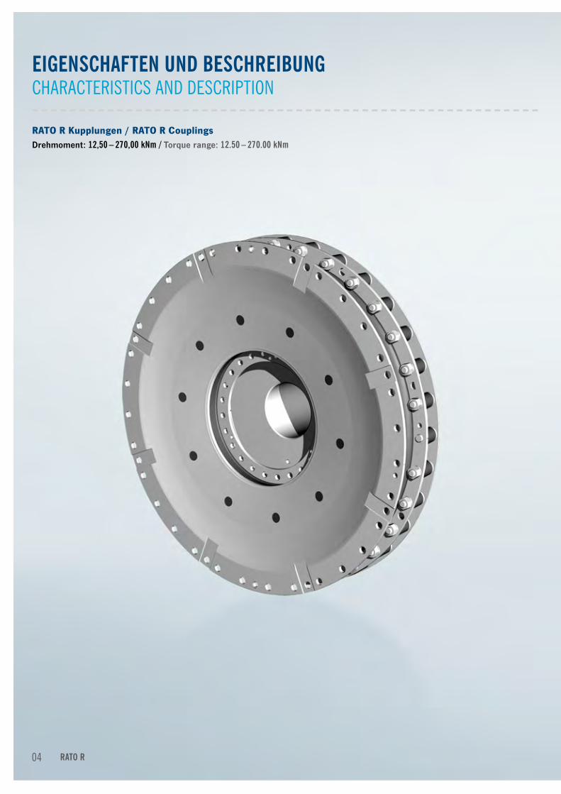
eiGensChaften und BesChReiBunGcharacTerisTics anD DescripTiOn
RATO R Kupplungen / RATO R CouplingsDrehmoment: 12,50 – 270,00 knm / Torque range: 12.50 – 270.00 knm
04 RatO R
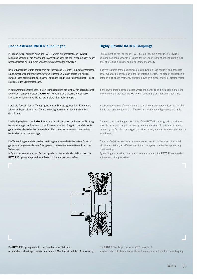
Hochelastische RATO R Kupplungen
In Ergänzung zur Allround-Kupplung RATO S wurde die hochelastische RATO R Kupplung speziell für die Anwendung in Antriebsanlagen mit der Forderung nach hoher Drehnachgiebigkeit und guten Verlagerungseigenschaften entwickelt.
Bei der Konzeption wurde großer Wert auf thermische Sicherheit und gute dynamische Laufeigenschaften mit möglichst geringen rotierenden Massen gelegt. Die Anwen-dungen liegen somit vorrangig in schnelllaufenden Haupt- und Nebenantrieben – seien es diesel- oder elektromotorische.
In den Drehmomentbereichen, die ein Handhaben und den Einbau von geschlossenen Elementen gestatten, bietet die RATO Ring Kupplung eine zusätzliche Alternative. Dieses ist vornehmlich bei kleinen bis mittleren Baugrößen möglich.
Durch die Auswahl der zur Verfügung stehenden Drehsteifigkeiten bzw. Elementaus-führungen lässt sich eine gute Drehschwingungsabstimmung der Antriebsanlage durchführen.
Die Nachgiebigkeiten der RATO R Kupplung in radialer, axialer und winkliger Richtung bei kürzestmöglicher Baulänge sorgen für einen günstigen Ausgleich der Wellenverla-gerungen bei elastischer Motoraufstellung, Fundamentveränderungen oder anderen betriebsbedingten Verlagerungen.
Die Verwendung von relativ weichen Kreisringmembranen bietet bei axialer Schwin-gungsanregung eine wirksame Entkoppelung und somit einen effektiven Schutz der Wellenlager.Aufgrund der Vermeidung von Geräuschpfaden – direkter Metallkontakt – bietet die RATO R Kupplung ausgezeichnete Geräuschdämmungseigenschaften.
Highly Flexible RATO R Couplings
Complementing the ”all-round“ RATO S coupling, the highly flexible RATO R coupling has been specially designed for the use in installations requiring a high level of torsional flexibility and misalignment capacity.
Inherent features of the design include high dynamic load capacity and good rota-tional dynamic properties due to the low rotating inertias. The area of application is primarily high-speed main/PTO systems driven by a diesel engine or electric motor.
In the low to middle torque ranges where the handling and installation of a com-plete element is practical the RATO Ring coupling is an additional alternative.
A customized tuning of the system’s torsional vibration characteristics is possible due to the variety of torsional stiffnesses and element configurations available.
The radial, axial and angular flexibility of the RATO R coupling, with the shortest possible installation length, enables good compensation of shaft misalignments caused by the flexible mounting of the prime mover, foundation movements etc. to be achieved.
The use of relatively soft annular membranes permits, in the event of an axial vibration excitation, an efficient isolation of the system – effectively protecting shaft bearings.By avoiding noise paths, direct metal to metal contact, the RATO R has excellent noise-attenuation properties.
Die RATO R Kupplung besteht in der Basisbaureihe 2200 aus:Anbaunabe, mehrreihigem elastischen Element, Membranteil und dem Anschlussring.
The RATO R Coupling in the series 2200 consists of:attached hub, multiple-row flexible element, membrane part and the connecting ring.
05RatO R
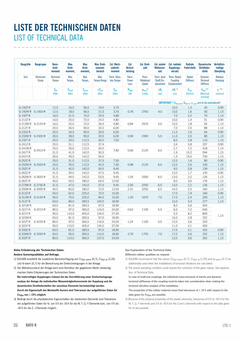
liste deR teChnisChen datenlisT Of Technical DaTa
Baugröße Baugruppe nenn-dreh-
moment
max.dreh-
moment 1
max.dreh-
moment 2
max. dreh-moment-bereich
zul. Wech-seldreh-moment
zul. Verlust-leistung
zul. dreh-zahl
zul. axialer Wellenver-
satz
zul. radialer kupplungs-
versatz
Radiale federsteife
dynamische drehfeder-
steife
Verhältnis-mäßige
dämpfung
size Dimension Group
norminal Torque
max.Torque1
max.Torque2
max. Torque range
perm. Vibra-tory Torque
perm. power loss
perm. rotational
speed
perm. axial shaft Dis-placement
perm. radial coupling
Displacement
radial stiffness
Dynamic Torsional stiffness
relative Damping
tkn knm
tkmax1 knm
tkmax2 knm
∆tmax knm
tkW knm
PkV50 kW
nkmax2)
1/min∆ka mm
∆kr‘ 2) mm
Crdyn kn/mm
Ctdyn1) 2)
knm/rad nominal
ψ 1) 3) nominal
imPORtant1): Ctdyn warm, Ctdyn la, ψ warm are to be considered!
G 192Z RG 1920 R
12,5 16,0 56,5 19,0 3,750,76 2750 4,0
10,0 1,3 40 0,90G 192W R 12,5 18,0 56,5 21,5 3,75 10,0 1,6 50 1,13G 192T R 16,0 21,5 72,0 25,5 4,80 7,0 2,2 70 1,13G 212Z R
G 2120 R16,0 20,0 72,0 24,0 4,80
0,84 2525 5,010,0 1,4 51 0,90
G 212W R 16,0 22,0 72,0 26,5 4,80 10,0 1,8 64 1,13G 212T R 20,0 26,5 90,0 32,0 6,00 7,0 2,5 88 1,13G 232Z R
G 2320 R20,0 24,5 90,0 29,5 6,00
0,90 2350 5,511,0 1,6 64 0,90
G 232W R 20,0 28,0 90,0 33,5 6,00 11,0 2,0 80 1,13G 232T R 25,0 33,5 112,5 40,0 7,50 8,0 2,8 110 1,13G 241Z R
G 2410 R
25,0 31,1 112,5 37,4
7,80 0,66 2125 6,0
3,4 5,8 337 0,90G 241W R 25,0 35,0 112,5 42,0 2,7 7,2 418 1,13G 241T R 31,5 41,9 142,0 50,3 1,9 10,2 594 1,13G 241Y R 35,6 45,0 142,0 54,0 1,3 15,0 730 1,13G 252Z R
G 2520 R25,0 31,0 112,5 37,5 7,50
0,98 2125 6,012,0 1,6 80 0,90
G 252W R 25,0 35,0 112,5 42,0 7,50 12,0 2,0 100 1,13G 252T R 31,5 42,0 142,0 50,5 9,45 9,0 2,8 139 1,13G 262Z R
G 2620 R31,5 39,5 142,0 47,5 9,45
1,05 2000 6,013,0 1,7 100 0,90
G 262W R 31,5 44,5 142,0 53,5 9,45 13,0 2,2 126 1,13G 262T R 40,0 53,5 180,0 64,0 12,00 9,0 3,0 176 1,13G 273W R G 2730 R 31,5 47,5 142,0 57,0 9,45 2,00 2250 6,0 13,0 2,2 126 1,13G 293W R G 2930 R 40,0 60,0 180,0 72,0 12,00 2,31 2250 6,0 14,0 2,5 160 1,13G 312Z R
G 3120 R50,0 62,5 225,0 75,0 15,00
1,20 1675 7,017,0 1,9 160 0,90
G 312W R 50,0 70,0 225,0 84,0 15,00 17,0 2,4 200 1,13G 312T R 63,0 84,0 283,5 100,5 18,90 12,0 3,3 277 1,13G 321W R
G 3210 R63,0 81,0 283,5 97,0 18,90
0,62 1100 5,58,0 5,6 504
1,13
G 321T R 80,0 97,0 360,0 116,5 24,00 6,0 7,2 640G 321Y R 90,0 110,5 405,0 134,0 27,00 5,5 8,2 800G 322W R
G 3220 R63,0 81,0 283,5 97,0 18,90
1,24 1100 5,516,0 2,8 252
G 322T R 80,0 97,0 360,0 116,5 24,00 12,0 3,6 320G 322Y R 90,0 110,5 405,0 134,0 27,00 11,0 4,1 400G 333Z R
G 3330 R63,0 81,0 283,5 97,0 18,90
2,70 1725 7,017,0 2,1 202 0,90
G 333W R 63,0 95,0 283,5 114,0 18,90 17,0 2,6 252 1,13G 333T R 80,0 114,0 360,0 137,0 24,00 12,0 3,6 352 1,13
Siehe Erläuterung der Technischen Daten.
Andere Gummiqualitäten auf Anfrage.
1) VULKAN empfiehlt die zusätzliche Berücksichtigung von CTdyn warm (0,7), CTdyn la (1,35)
und ψ warm (0,7) für die Berechnung der Drehschwingungen in der Anlage.
2) Der Betriebszustand der Anlage kann eine Korrektur der gegebenen Werte notwendig
machen.Siehe Erläuterungen der Technischen Daten.
Bei mehrreihigen Kupplungen müssen bei der Durchführung einer Drehschwingungs-
analyse der Anlage die individuellen Massenträgheitsmomente der Kupplung und die
dynamischen Drehfedersteifen der einzelnen Elemente berücksichtigt werden.
Durch die Eigenschaft des Werkstoffs Gummi sind Toleranzen der aufgeführten Daten für
CTdyn von ± 15% möglich.
3) Bedingt durch die physikalischen Eigenschaften der elastischen Elemente sind Toleranzen
der aufgeführten Daten für ψ, von 0 % bis -30 % für die W, T, Q, Y Elemente bzw., von 0 % bis
-45 % für die Z, J Elemente möglich.
See Explanation of the Technical Data.
Different rubber qualities on request.
1) VULKAN recommend that the values CTdyn warm (0.7), CTdyn la (1.35) and ψ warm (0.7) be
additionally used when the installations of torsional vibrations are calculated.
2) The actual operating condition could require the correction of the given values. See explana-
tion of Technical Data.
In case of multi-row couplings, the individual mass-moments of inertia and dynamic
torsional stiffnesses of the coupling must be taken into consideration when making the
torsional vibration analysis of the installation.
The properties of the rubber material mean that tolerances of ± 15 % with respect to the
data given for CTdyn are possible.
3) Because of the physical properties of the elastic elements, tolerances of 0 % to -30 % for the
W, T, Q, Y elements and 0 % to -45 % for the Z and J elements with respect to the data given
for ψ are possible.
lTD-106 RatO R
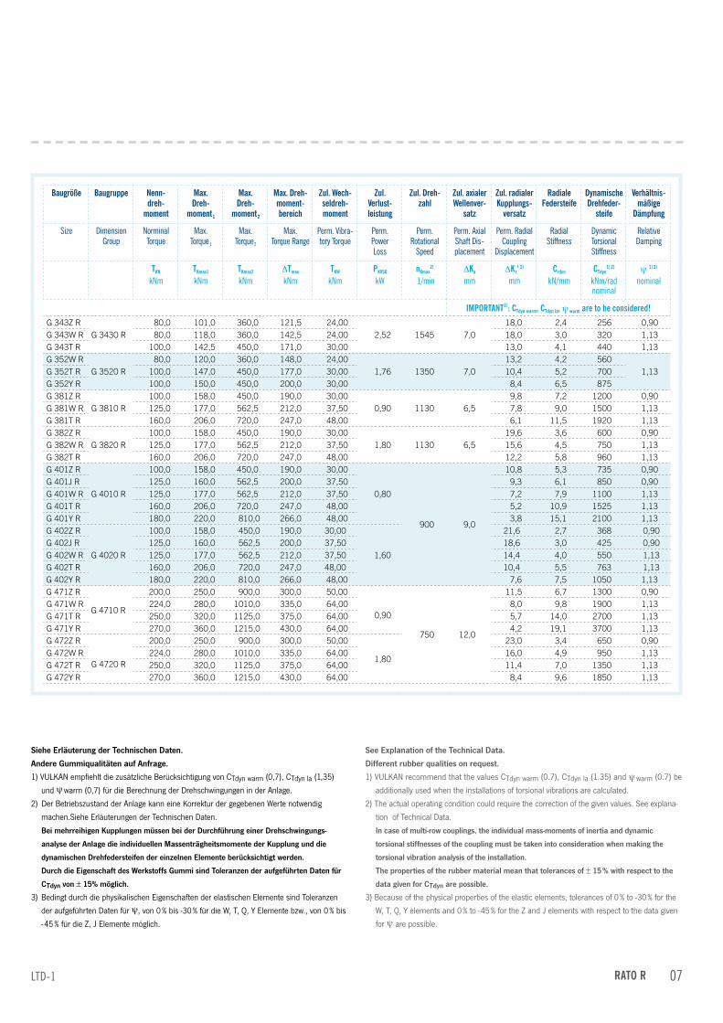
Baugröße Baugruppe nenn-dreh-
moment
max.dreh-
moment1
max.dreh-
moment2
max. dreh-moment-bereich
zul. Wech-seldreh-moment
zul. Verlust-leistung
zul. dreh-zahl
zul. axialer Wellenver-
satz
zul. radialer kupplungs-
versatz
Radiale federsteife
dynamische drehfeder-
steife
Verhältnis-mäßige
dämpfung
size Dimension Group
norminal Torque
max.Torque1
max.Torque2
max. Torque range
perm. Vibra-tory Torque
perm. power loss
perm. rotational
speed
perm. axial shaft Dis-placement
perm. radial coupling
Displacement
radial stiffness
Dynamic Torsional stiffness
relative Damping
tkn knm
tkmax1 knm
tkmax2 knm
∆tmax knm
tkW knm
PkV50 kW
nkmax2)
1/min∆ka mm
∆kr‘ 2) mm
Crdyn kn/mm
Ctdyn1) 2)
knm/rad nominal
ψ 1) 3) nominal
imPORtant1): Ctdyn warm, Ctdyn la, ψ warm are to be considered!
G 343Z RG 3430 R
80,0 101,0 360,0 121,5 24,002,52 1545 7,0
18,0 2,4 256 0,90G 343W R 80,0 118,0 360,0 142,5 24,00 18,0 3,0 320 1,13G 343T R 100,0 142,5 450,0 171,0 30,00 13,0 4,1 440 1,13G 352W R
G 3520 R80,0 120,0 360,0 148,0 24,00
1,76 1350 7,013,2 4,2 560
1,13G 352T R 100,0 147,0 450,0 177,0 30,00 10,4 5,2 700G 352Y R 100,0 150,0 450,0 200,0 30,00 8,4 6,5 875G 381Z R
G 3810 R100,0 158,0 450,0 190,0 30,00
0,90 1130 6,59,8 7,2 1200 0,90
G 381W R 125,0 177,0 562,5 212,0 37,50 7,8 9,0 1500 1,13G 381T R 160,0 206,0 720,0 247,0 48,00 6,1 11,5 1920 1,13G 382Z R
G 3820 R100,0 158,0 450,0 190,0 30,00
1,80 1130 6,519,6 3,6 600 0,90
G 382W R 125,0 177,0 562,5 212,0 37,50 15,6 4,5 750 1,13G 382T R 160,0 206,0 720,0 247,0 48,00 12,2 5,8 960 1,13G 401Z R
G 4010 R
100,0 158,0 450,0 190,0 30,00
0,80
900 9,0
10,8 5,3 735 0,90G 401J R 125,0 160,0 562,5 200,0 37,50 9,3 6,1 850 0,90G 401W R 125,0 177,0 562,5 212,0 37,50 7,2 7,9 1100 1,13G 401T R 160,0 206,0 720,0 247,0 48,00 5,2 10,9 1525 1,13G 401Y R 180,0 220,0 810,0 266,0 48,00 3,8 15,1 2100 1,13G 402Z R
G 4020 R
100,0 158,0 450,0 190,0 30,00
1,60
21,6 2,7 368 0,90G 402J R 125,0 160,0 562,5 200,0 37,50 18,6 3,0 425 0,90G 402W R 125,0 177,0 562,5 212,0 37,50 14,4 4,0 550 1,13G 402T R 160,0 206,0 720,0 247,0 48,00 10,4 5,5 763 1,13G 402Y R 180,0 220,0 810,0 266,0 48,00 7,6 7,5 1050 1,13G 471Z R
G 4710 R
200,0 250,0 900,0 300,0 50,00
0,90
750 12,0
11,5 6,7 1300 0,90G 471W R 224,0 280,0 1010,0 335,0 64,00 8,0 9,8 1900 1,13G 471T R 250,0 320,0 1125,0 375,0 64,00 5,7 14,0 2700 1,13G 471Y R 270,0 360,0 1215,0 430,0 64,00 4,2 19,1 3700 1,13G 472Z R
G 4720 R
200,0 250,0 900,0 300,0 50,00
1,80
23,0 3,4 650 0,90G 472W R 224,0 280,0 1010,0 335,0 64,00 16,0 4,9 950 1,13G 472T R 250,0 320,0 1125,0 375,0 64,00 11,4 7,0 1350 1,13G 472Y R 270,0 360,0 1215,0 430,0 64,00 8,4 9,6 1850 1,13
Siehe Erläuterung der Technischen Daten.
Andere Gummiqualitäten auf Anfrage.
1) VULKAN empfiehlt die zusätzliche Berücksichtigung von CTdyn warm (0,7), CTdyn la (1,35)
und ψ warm (0,7) für die Berechnung der Drehschwingungen in der Anlage.
2) Der Betriebszustand der Anlage kann eine Korrektur der gegebenen Werte notwendig
machen.Siehe Erläuterungen der Technischen Daten.
Bei mehrreihigen Kupplungen müssen bei der Durchführung einer Drehschwingungs-
analyse der Anlage die individuellen Massenträgheitsmomente der Kupplung und die
dynamischen Drehfedersteifen der einzelnen Elemente berücksichtigt werden.
Durch die Eigenschaft des Werkstoffs Gummi sind Toleranzen der aufgeführten Daten für
CTdyn von ± 15% möglich.
3) Bedingt durch die physikalischen Eigenschaften der elastischen Elemente sind Toleranzen
der aufgeführten Daten für ψ, von 0 % bis -30 % für die W, T, Q, Y Elemente bzw., von 0 % bis
-45 % für die Z, J Elemente möglich.
See Explanation of the Technical Data.
Different rubber qualities on request.
1) VULKAN recommend that the values CTdyn warm (0.7), CTdyn la (1.35) and ψ warm (0.7) be
additionally used when the installations of torsional vibrations are calculated.
2) The actual operating condition could require the correction of the given values. See explana-
tion of Technical Data.
In case of multi-row couplings, the individual mass-moments of inertia and dynamic
torsional stiffnesses of the coupling must be taken into consideration when making the
torsional vibration analysis of the installation.
The properties of the rubber material mean that tolerances of ± 15 % with respect to the
data given for CTdyn are possible.
3) Because of the physical properties of the elastic elements, tolerances of 0 % to -30 % for the
W, T, Q, Y elements and 0 % to -45 % for the Z and J elements with respect to the data given
for ψ are possible.
lTD-1 07RatO R

Baugruppe abmessungen massenträgheitsmoment masse schwerpunktsabstand
Dimension Group
Dimensions mass moment of inertia mass Distance to center of gravity
tkn d1 d2 d3 d4 z lkr t l1 l2 l4 l5 l8 J1 J2 J3 J4 m1 m2 m3 m4 s1 s2 s3 s4
knm vorgeb.pilot bored
max [kgm2] [kg] [mm]
G1920R 12,5 -16,0
595 70 150 13,5 – 585 558 32 346,95 175,0 12,5 – – 1,0 1,3 2,5 – 24,00 26,0 97,00 – 27,0 266,0 139 –
G2120R 16,0 -20,0
640 80 160 13,5 – 635 608 32 390,00 185,0 8,0 – – 1,3 1,8 3,0 – 24,00 32,0 106,00 – 23,0 302,0 152 –
G2320R 20,0 -25,0
685 110 170 15,5 – 680 650 32 411,00 195,0 10,0 – – 2,0 2,5 4,4 – 33,00 38,0 123,00 – 25,0 317,0 166 –
G2410R 25,0 -35,6
735 110 185 17,5 – 740 700 32 324,70 225,0 8,0 – – 2,1 5,4 – – 30,00 147,0 – – 13,0 172,0 – –
G2520R 25,0 -31,5
735 110 185 15,5 – 730 700 32 463,00 225,0 10,0 – – 2,8 3,4 6,0 – 40,00 45,0 161,00 – 34,0 360,0 191 –
G2620R 31,5 -40,0
793 100 200 17,5 – 790 755 32 488,00 235,0 10,0 – – 3,9 4,8 9,1 – 47,00 55,0 207,00 – 28,0 378,0 191 –
G2730R 31,5 800 100 200 17,5 28,0 790 755 32 500,00 235,0 32,0 6 21,0 7,6 4,0 4,0 9,60 78,00 44,0 44,00 217 52,0 114,0 330 174,0
G2930R 40,0 870 110 220 20,0 32,0 860 820 32 535,00 250,0 35,0 6 23,0 11,7 6,0 6,0 14,90 103,00 55,0 55,00 283 57,0 123,0 352 185,0
G3110R 50,0 -63,0
920 115 235 20,0 – 920 880 32 452,20 285,0 12,0 – – 8,5 15,5 – – 77,00 296,0 – – 34,0 209,0 – –
G3120R 50,0 -63,0
920 115 235 20,0 – 920 880 32 586,00 285,0 12,0 – – 8,5 10,6 19,5 – 77,00 91,0 333,00 – 34,0 454,0 228 –
G3210R 63,0 -90,0
1000 150 255 22,0 – 995 950 32 497,50 300,0 12,0 – – 12,9 29,1 – – 96,00 403,0 – – 30,0 243,0 – –
G3220R 63,0 -90,0
1000 150 255 22,0 – 995 950 32 656,00 300,0 12,0 – – 12,9 28,1 29,1 – 100,00 202,0 404,00 – 30,0 499,0 243 –
G3330R 63,0 -80,0
1010 125 255 22,0 36,0 995 950 32 635,00 300,0 40,0 8 25,0 24,8 12,5 13,0 30,70 157,00 90,0 90,00 434 64,0 143,0 419 220,0
G3430R 80,0 -100,0
1085 160 275 24,0 39,0 1070 1025 32 670,00 310,0 45,0 8 28,0 28,0 21,4 21,0 42,30 157,00 128,0 127,00 524 55,0 523,0 424 236,0
G3520R 80,0 -100,0
1135 135 275 24,0 – 1120 1075 32 597,15 310,0 11,4 – – 16,1 17,9 59,4 – 92,00 146,0 597,00 – 25,0 470,0 253 –
G4010R 100,0 -180,0
1250 220 320 26,0 – 1240 1190 32 626,00 385,0 14,0 – – 38,3 83,5 – – 184,00 768,0 – – 36,0 307,0 – –
G4020R 100,0 -180,0
1250 200 320 26,0 – 1240 1190 32 821,50 385,0 14,0 – – 38,5 82,9 84,0 – 190,00 385,0 770,00 – 37,0 628,0 307 –
G4710R 200,0 -270,0
1465 230 370 32,0 – 1460 1395 32 736,60 480,0 14,0 – – 74,7 173,6 – – 274,00 1222,0 – – 38,5 367,0 – –
G4720R 200,0 -270,0
1465 230 370 32,0 – 1460 1395 32 953,60 480,0 14,0 – – 74,7 166,0 173,6 – 274,00 559,0 1228,00 – 38,5 742,0 369 –
aBmessunGen/massentRäGheitsmOmente/massenDimensiOns/mass-mOmenTs Of inerTia/masses
Maße in mm
Alle Massen und Massenträgheitsmomente beziehen sich auf vorgebohrte Naben. Bei mehrrei-
higen Kupplungen müssen bei der Durchführung einer Drehschwingungsanalyse der Anlage die
individuellen Massenträgheitsmomente der Kupplung und die dynamischen Drehfedersteifen
der einzelnen Elemente berück- sichtigt werden.
Dimensions in mm
All masses and mass moments of inertia refer to pilot bored hubs. In case of multi-row
couplings the individual mass-moments of inertia and dynamic torsional stiffnesses of the
coupling must be taken into consideration when making the torsional vibration analysis of the
installation.
RATO R Baureihe / Series 2200
a/m 2200-208 RatO R
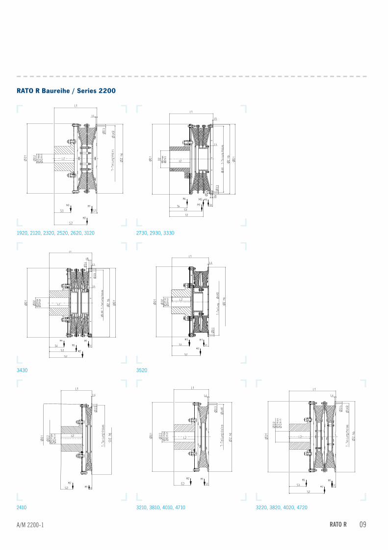
RATO R Baureihe / Series 2200
1920, 2120, 2320, 2520, 2620, 3120 2730, 2930, 3330
3430 3520
2410 3210, 3810, 4010, 4710 3220, 3820, 4020, 4720
a/m 2200-1 09RatO R
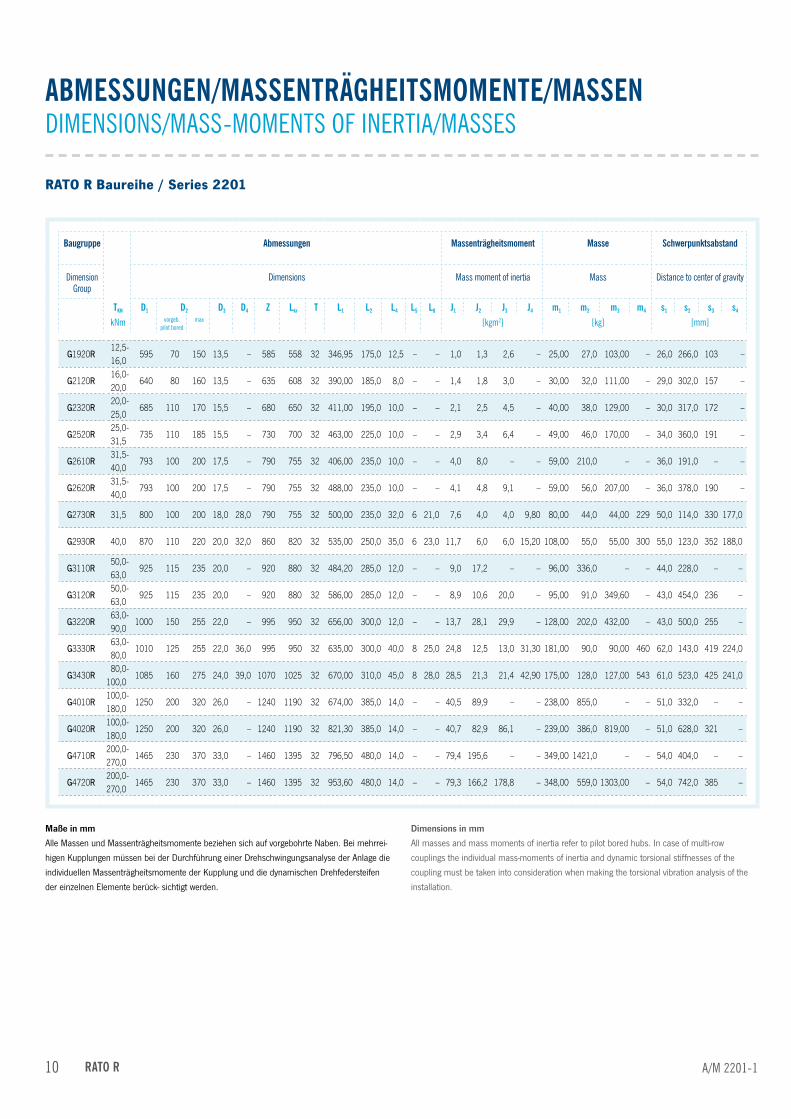
aBmessunGen/massentRäGheitsmOmente/massenDimensiOns/mass-mOmenTs Of inerTia/masses
Baugruppe abmessungen massenträgheitsmoment masse schwerpunktsabstand
Dimension Group
Dimensions mass moment of inertia mass Distance to center of gravity
tkn d1 d2 d3 d4 z lkr t l1 l2 l4 l5 l8 J1 J2 J3 J4 m1 m2 m3 m4 s1 s2 s3 s4
knm vorgeb.pilot bored
max [kgm2] [kg] [mm]
G1920R12,5 -
595 70 150 13,5 – 585 558 32 346,95 175,0 12,5 – – 1,0 1,3 2,6 – 25,00 27,0 103,00 – 26,0 266,0 103 –16,0
G2120R16,0 -
640 80 160 13,5 – 635 608 32 390,00 185,0 8,0 – – 1,4 1,8 3,0 – 30,00 32,0 111,00 – 29,0 302,0 157 –20,0
G2320R20,0 -
685 110 170 15,5 – 680 650 32 411,00 195,0 10,0 – – 2,1 2,5 4,5 – 40,00 38,0 129,00 – 30,0 317,0 172 –25,0
G2520R25,0 -
735 110 185 15,5 – 730 700 32 463,00 225,0 10,0 – – 2,9 3,4 6,4 – 49,00 46,0 170,00 – 34,0 360,0 191 –31,5
G2610R31,5 -
793 100 200 17,5 – 790 755 32 406,00 235,0 10,0 – – 4,0 8,0 – – 59,00 210,0 – – 36,0 191,0 – –40,0
G2620R31,5-
793 100 200 17,5 – 790 755 32 488,00 235,0 10,0 – – 4,1 4,8 9,1 – 59,00 56,0 207,00 – 36,0 378,0 190 –40,0
G2730R 31,5 800 100 200 18,0 28,0 790 755 32 500,00 235,0 32,0 6 21,0 7,6 4,0 4,0 9,80 80,00 44,0 44,00 229 50,0 114,0 330 177,0
G2930R 40,0 870 110 220 20,0 32,0 860 820 32 535,00 250,0 35,0 6 23,0 11,7 6,0 6,0 15,20 108,00 55,0 55,00 300 55,0 123,0 352 188,0
G3110R50,0 -
925 115 235 20,0 – 920 880 32 484,20 285,0 12,0 – – 9,0 17,2 – – 96,00 336,0 – – 44,0 228,0 – –63,0
G3120R50,0 -
925 115 235 20,0 – 920 880 32 586,00 285,0 12,0 – – 8,9 10,6 20,0 – 95,00 91,0 349,60 – 43,0 454,0 236 –63,0
G3220R63,0 -
1000 150 255 22,0 – 995 950 32 656,00 300,0 12,0 – – 13,7 28,1 29,9 – 128,00 202,0 432,00 – 43,0 500,0 255 –90,0
G3330R63,0 -
1010 125 255 22,0 36,0 995 950 32 635,00 300,0 40,0 8 25,0 24,8 12,5 13,0 31,30 181,00 90,0 90,00 460 62,0 143,0 419 224,080,0
G3430R80,0 -
1085 160 275 24,0 39,0 1070 1025 32 670,00 310,0 45,0 8 28,0 28,5 21,3 21,4 42,90 175,00 128,0 127,00 543 61,0 523,0 425 241,0100,0
G4010R100,0 -
1250 200 320 26,0 – 1240 1190 32 674,00 385,0 14,0 – – 40,5 89,9 – – 238,00 855,0 – – 51,0 332,0 – –180,0
G4020R100,0 -
1250 200 320 26,0 – 1240 1190 32 821,30 385,0 14,0 – – 40,7 82,9 86,1 – 239,00 386,0 819,00 – 51,0 628,0 321 –180,0
G4710R200,0-
1465 230 370 33,0 – 1460 1395 32 796,50 480,0 14,0 – – 79,4 195,6 – – 349,00 1421,0 – – 54,0 404,0 – –270,0
G4720R200,0 -
1465 230 370 33,0 – 1460 1395 32 953,60 480,0 14,0 – – 79,3 166,2 178,8 – 348,00 559,0 1303,00 – 54,0 742,0 385 –270,0
RATO R Baureihe / Series 2201
Maße in mm
Alle Massen und Massenträgheitsmomente beziehen sich auf vorgebohrte Naben. Bei mehrrei-
higen Kupplungen müssen bei der Durchführung einer Drehschwingungsanalyse der Anlage die
individuellen Massenträgheitsmomente der Kupplung und die dynamischen Drehfedersteifen
der einzelnen Elemente berück- sichtigt werden.
Dimensions in mm
All masses and mass moments of inertia refer to pilot bored hubs. In case of multi-row
couplings the individual mass-moments of inertia and dynamic torsional stiffnesses of the
coupling must be taken into consideration when making the torsional vibration analysis of the
installation.
a/m 2201-110 RatO R
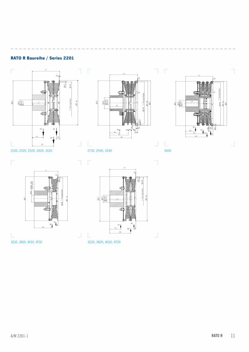
RATO R Baureihe / Series 2201
2120, 2320, 2520, 2620, 3120 2730, 2930, 3330 3430
3210, 3810, 4010, 4710 3220, 3820, 4020, 4720
a/m 2201-1 11RatO R
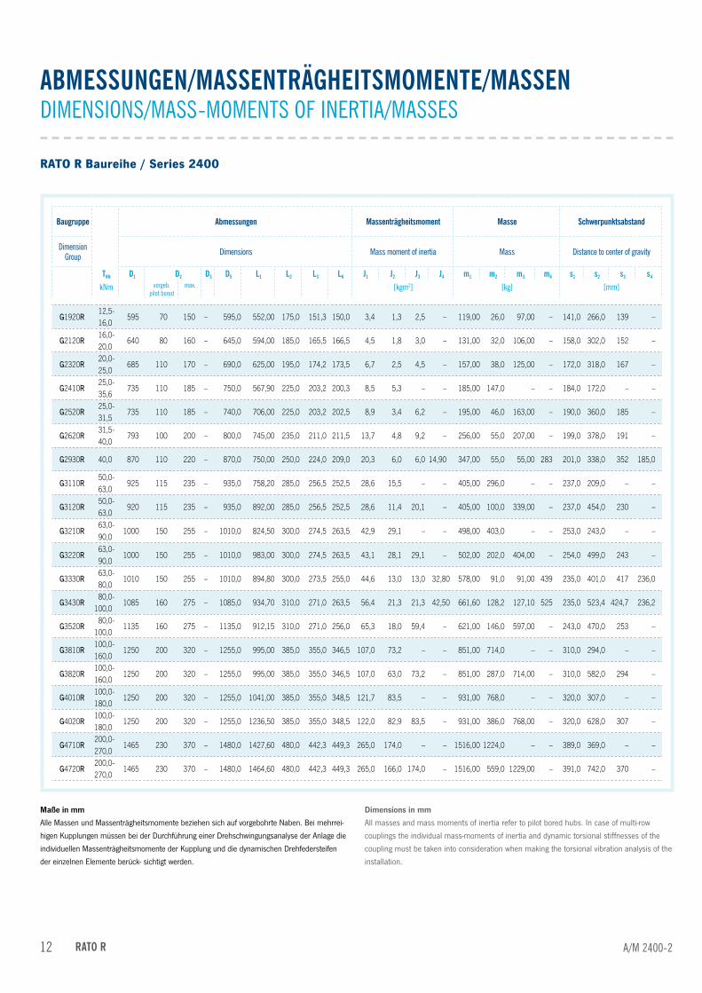
aBmessunGen/massentRäGheitsmOmente/massenDimensiOns/mass-mOmenTs Of inerTia/masses
Baugruppe abmessungen massenträgheitsmoment masse schwerpunktsabstand
Dimension Group Dimensions mass moment of inertia mass Distance to center of gravity
tkn d1 d2 d3 d5 l1 l2 l3 l6 J1 J2 J3 J4 m1 m2 m3 m4 s1 s2 s3 s4
knm vorgeb.pilot bored
max. [kgm2] [kg] [mm]
G1920R12,5 -
595 70 150 – 595,0 552,00 175,0 151,3 150,0 3,4 1,3 2,5 – 119,00 26,0 97,00 – 141,0 266,0 139 –16,0
G2120R16,0 -
640 80 160 – 645,0 594,00 185,0 165,5 166,5 4,5 1,8 3,0 – 131,00 32,0 106,00 – 158,0 302,0 152 –20,0
G2320R20,0 -
685 110 170 – 690,0 625,00 195,0 174,2 173,5 6,7 2,5 4,5 – 157,00 38,0 125,00 – 172,0 318,0 167 –25,0
G2410R25,0 -
735 110 185 – 750,0 567,90 225,0 203,2 200,3 8,5 5,3 – – 185,00 147,0 – – 184,0 172,0 – –35,6
G2520R25,0 -
735 110 185 – 740,0 706,00 225,0 203,2 202,5 8,9 3,4 6,2 – 195,00 46,0 163,00 – 190,0 360,0 185 –31,5
G2620R31,5-
793 100 200 – 800,0 745,00 235,0 211,0 211,5 13,7 4,8 9,2 – 256,00 55,0 207,00 – 199,0 378,0 191 –40,0
G2930R 40,0 870 110 220 – 870,0 750,00 250,0 224,0 209,0 20,3 6,0 6,0 14,90 347,00 55,0 55,00 283 201,0 338,0 352 185,0
G3110R50,0 -
925 115 235 – 935,0 758,20 285,0 256,5 252,5 28,6 15,5 – – 405,00 296,0 – – 237,0 209,0 – –63,0
G3120R50,0 -
920 115 235 – 935,0 892,00 285,0 256,5 252,5 28,6 11,4 20,1 – 405,00 100,0 339,00 – 237,0 454,0 230 –63,0
G3210R63,0 -
1000 150 255 – 1010,0 824,50 300,0 274,5 263,5 42,9 29,1 – – 498,00 403,0 – – 253,0 243,0 – –90,0
G3220R63,0 -
1000 150 255 – 1010,0 983,00 300,0 274,5 263,5 43,1 28,1 29,1 – 502,00 202,0 404,00 – 254,0 499,0 243 –90,0
G3330R63,0 -
1010 150 255 – 1010,0 894,80 300,0 273,5 255,0 44,6 13,0 13,0 32,80 578,00 91,0 91,00 439 235,0 401,0 417 236,080,0
G3430R80,0-
1085 160 275 – 1085,0 934,70 310,0 271,0 263,5 56,4 21,3 21,3 42,50 661,60 128,2 127,10 525 235,0 523,4 424,7 236,2100,0
G3520R80,0 -
1135 160 275 – 1135,0 912,15 310,0 271,0 256,0 65,3 18,0 59,4 – 621,00 146,0 597,00 – 243,0 470,0 253 –100,0
G3810R100,0-
1250 200 320 – 1255,0 995,00 385,0 355,0 346,5 107,0 73,2 – – 851,00 714,0 – – 310,0 294,0 – –160,0
G3820R100,0-
1250 200 320 – 1255,0 995,00 385,0 355,0 346,5 107,0 63,0 73,2 – 851,00 287,0 714,00 – 310,0 582,0 294 –160,0
G4010R100,0-
1250 200 320 – 1255,0 1041,00 385,0 355,0 348,5 121,7 83,5 – – 931,00 768,0 – – 320,0 307,0 – –180,0
G4020R100,0-
1250 200 320 – 1255,0 1236,50 385,0 355,0 348,5 122,0 82,9 83,5 – 931,00 386,0 768,00 – 320,0 628,0 307 –180,0
G4710R200,0-
1465 230 370 – 1480,0 1427,60 480,0 442,3 449,3 265,0 174,0 – – 1516,00 1224,0 – – 389,0 369,0 – –270,0
G4720R200,0-
1465 230 370 – 1480,0 1464,60 480,0 442,3 449,3 265,0 166,0 174,0 – 1516,00 559,0 1229,00 – 391,0 742,0 370 –270,0
RATO R Baureihe / Series 2400
Maße in mm
Alle Massen und Massenträgheitsmomente beziehen sich auf vorgebohrte Naben. Bei mehrrei-
higen Kupplungen müssen bei der Durchführung einer Drehschwingungsanalyse der Anlage die
individuellen Massenträgheitsmomente der Kupplung und die dynamischen Drehfedersteifen
der einzelnen Elemente berück- sichtigt werden.
Dimensions in mm
All masses and mass moments of inertia refer to pilot bored hubs. In case of multi-row
couplings the individual mass-moments of inertia and dynamic torsional stiffnesses of the
coupling must be taken into consideration when making the torsional vibration analysis of the
installation.
a/m 2400-212 RatO R
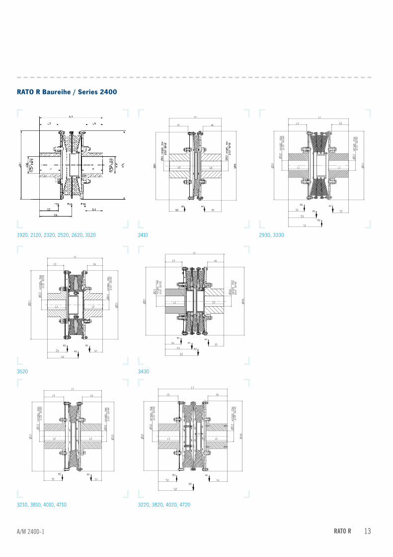
RATO R Baureihe / Series 2400
2930, 3330
3520 3430
3210, 3810, 4010, 4710 3220, 3820, 4020, 4720
24101920, 2120, 2320, 2520, 2620, 3120
a/m 2400-1 13RatO R

210
220
200
190
180
170
160
150
140
130
120
110
100
9080
7060
5040
3020
100
nOtizennOTice
14 RatO R

nOtizennOTice
210
220
200
190
180
170
160
150
140
130
120
110
100
9080
7060
5040
3020
100
15RatO R

Head Office: VULKAN Kupplungs- und Getriebebau Bernhard Hackforth GmbH & Co. KG | Heerstraße 66 | 44653 Herne | GermanyPhone + 49 (0) 2325 922-0 | Fax + 49 (0) 2325 71110 | Mail [email protected]
www.vulkan.com

Cedervall sterntube bearings
For technical specification, see back-cover of this leaflet.
The Cedervall sterntube bearing together with Cedervall's world known seals forms a combination, which guaranties trouble free operation throughout the lifetime of your vessel.
Cedervall sterntube bearings are made of highest quality steel, cast iron or heavy duty ductile iron with centrifugally lined lead or tin based white metal.
Cedervall sterntube bearings can be supplied in standard sizes or to customer specification.The bearings can be machined for temperature sensors and a wide range of sensor types can be supplied as option.
www.cedervall.com
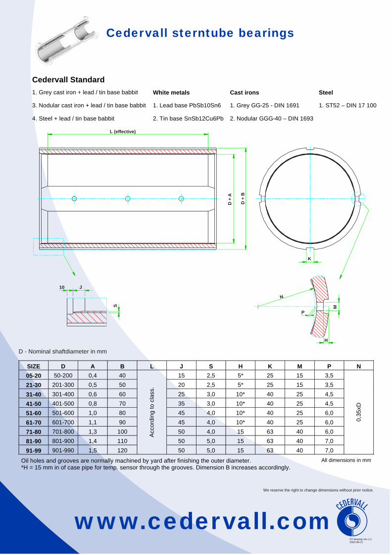
www.cedervall.com
Cedervall sterntube bearings
ST-bearing Ver 1.12003-08-21
L (effective)
K
P
J10
S
HM
D +
A
N
D +
B
SIZE D A B L J S H K M P N
05-20 50-200 0,4 40 15 2,5 5* 25 15 3,5
21-30 201-300 0,5 50 20 2,5 5* 25 15 3,5
31-40 301-400 0,6 60 25 3,0 10* 40 25 4,5
41-50 401-500 0,8 70 35 3,0 10* 40 25 4,5
51-60 501-600 1,0 80 45 4,0 10* 40 25 6,0
61-70 601-700 1,1 90 45 4,0 10* 40 25 6,0
71-80 701-800 1,3 100 50 4,0 15 63 40 6,0
81-90 801-900 1,4 110 50 5,0 15 63 40 7,0
91-99 901-990 1,5 120
Acco
rdin
gto
cla
ss.
50 5,0 15 63 40 7,0
0,3
5xD
Oil holes and grooves are normally machined by yard after finishing the outer diameter. *H = 15 mm in of case pipe for temp. sensor through the grooves. Dimension B increases accordingly.
All dimensions in mm
D - Nominal shaftdiameter in mm
Cedervall Standard
1. Grey cast iron + lead / tin base babbit White metals Cast irons Steel
3. Nodular cast iron + lead / tin base babbit 1. Lead base PbSb10Sn6 1. Grey GG-25 - DIN 1691 1. ST52 – DIN 17 100
4. Steel + lead / tin base babbit 2. Tin base SnSb12Cu6Pb 2. Nodular GGG-40 – DIN 1693
We reserve the right to change dimensions without prior notice.
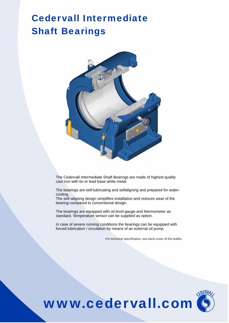
Cedervall Intermediate
Shaft Bearings
www.cedervall.com
For technical specification, see back-cover of this leaflet.
The Cedervall Intermediate Shaft Bearings are made of highest quality cast iron with tin or lead base white metal.
The bearings are self-lubricating and selfaligning and prepared for water-cooling.The self-aligning design simplifies installation and reduces wear of the bearing compared to conventional design.
The bearings are equipped with oil level gauge and thermometer as standard. Temperature sensor can be supplied as option.
In case of severe running conditions the bearings can be equipped with forced lubrication / circulation by means of an external oil pump.

Cedervall Intermediate Shaft Bearings
CHON Ver 1.22003-08-21
We reserve the right to change dimensions without prior notice.
*1. L = bearing length (Pos.3,4)*2. Item not shown in exploded view.*3. Optional item.
Partlist 1 Lower body 2 Upper body 3 Lower bearing 4 Upper bearing 5 Oil ring 6 Deflection ring 7 Guide pin 8 Assembly screw 9 Cover10 Spillway11 Oil level / Drain
*3( )12 Temperature sensor 13 Inlet / outlet cooling circuit14 Anti rotation pin15 Eye bolt
*2,3( )16 Fastning bolt *2,3( )17 Level bolt
18 Local thermometer
11
18
3
17
16
5
1
12
9
15
7
14
10
2
6
6
8
4
13
G
D -
D1
J
H
M
F
E A
U
B
C
E
Size D - D1 A B C E F G H J L(*1)
M U
125 101 - 125 220 310 360 149,0 199 217 150 320
70 35 4-ø25
165 126 - 165 270 350 410 150,0 210 310 215 403 125 40 4-ø25
210
166 - 210 310 400 460 210,0 270 360 245 458 185 40 4-ø32
235 211 - 240 350 490 550 240,0 300 436 260 508 250 40 4-ø32
265 241 - 274 460 550 610 130,0 320 446 300 560 255 45 6-ø32
290 275 - 300 480 580 640 145,0 350 485 325 600 275 40 6-ø32
320 301 - 332 450 620 680 160,0 380 510 345 664 300 50 6-ø32
350 333 - 365 500 640 700 190,0 440 532 360 685 350 50 6-ø32
380 366 - 400 560 700 760 190,0 440 574 380 725 360 50 6-ø32
420 401 - 432 600 740 800 210,0 480 615 390 735 360 55 6-ø32
450 433 - 465 655 795 855 225,0 510 642 440 825 430 70 6-ø32
480 466 - 500 730 840 930 217,5 525 525 425 830 300 75 6-ø45
530 501 - 550 770 880 970 135,0 360 510 450 870 300 80 6-ø45
580 551 - 600 845 965 1065 222,5 545 565 515 995 320 80 6-ø55
630 601 - 650 775 1040 1160 236,0 592 612 560 1082 352 85 6-ø58
All dimensions in mm
www.cedervall.com
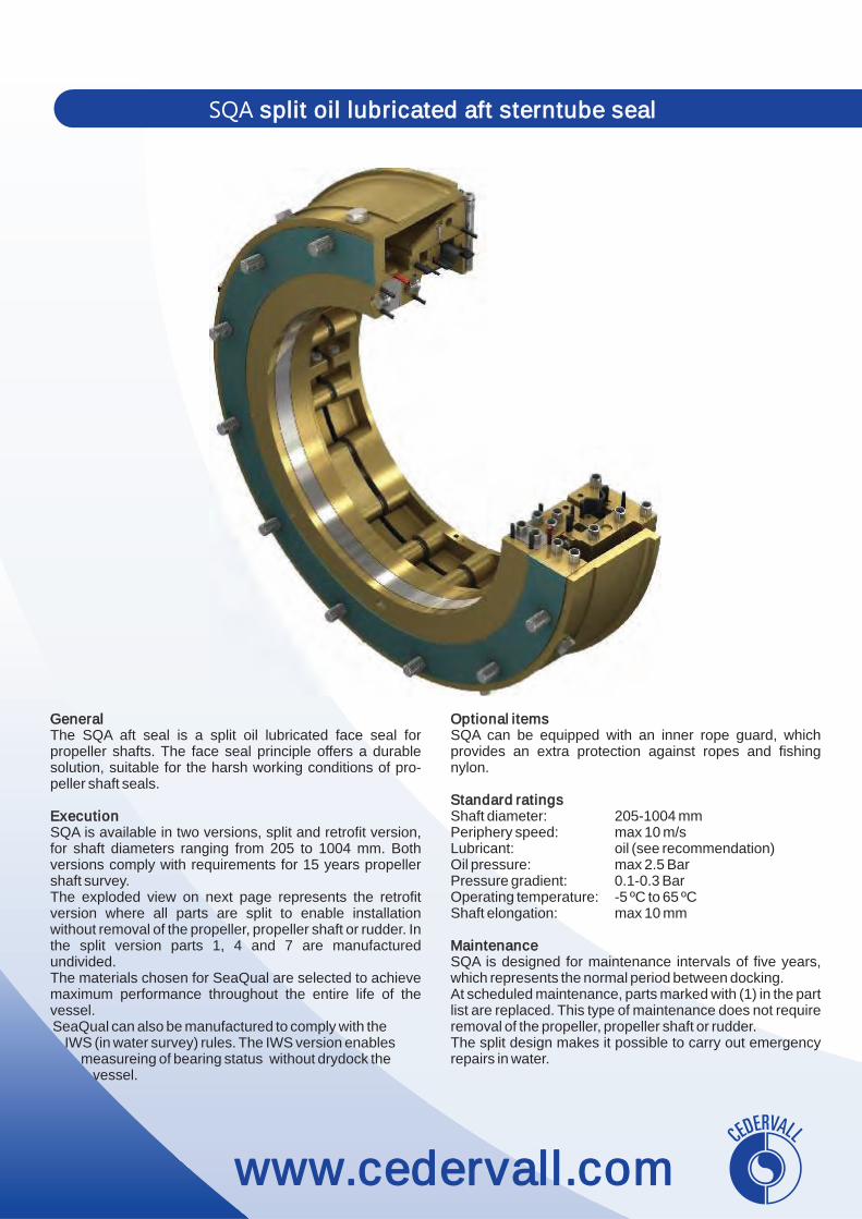
www.cedervall.com
GeneralThe SQA aft seal is a split oil lubricated face seal forpropeller shafts. The face seal principle offers a durablesolution, suitable for the harsh working conditions of pro-peller shaft seals.
ExecutionSQA is available in two versions, split and retrofit version,for shaft diameters ranging from 205 to 1004 mm. Bothversions comply with requirements for 15 years propellershaft survey.The exploded view on next page represents the retrofitversion where all parts are split to enable installationwithout removal of the propeller, propeller shaft or rudder. Inthe split version parts 1, 4 and 7 are manufacturedundivided.The materials chosen for SeaQual are selected to achievemaximum performance throughout the entire life of thevessel.SeaQual can also be manufactured to comply with the
IWS (in water survey) rules. The IWS version enablesmeasureing of bearing status without drydock the
vessel.
Optional itemsSQA can be equipped with an inner rope guard, whichprovides an extra protection against ropes and fishingnylon.
Standard ratingsShaft diameter: 205-1004 mmPeriphery speed: max 10 m/sLubricant: oil (see recommendation)Oil pressure: max 2.5 BarPressure gradient: 0.1-0.3 BarOperating temperature: -5 ºC to 65 ºCShaft elongation: max 10 mm
MaintenanceSQA is designed for maintenance intervals of five years,which represents the normal period between docking.At scheduled maintenance, parts marked with (1) in the partlist are replaced. This type of maintenance does not requireremoval of the propeller, propeller shaft or rudder.The split design makes it possible to carry out emergencyrepairs in water.
SQA split oil lubricated aft sterntube seal
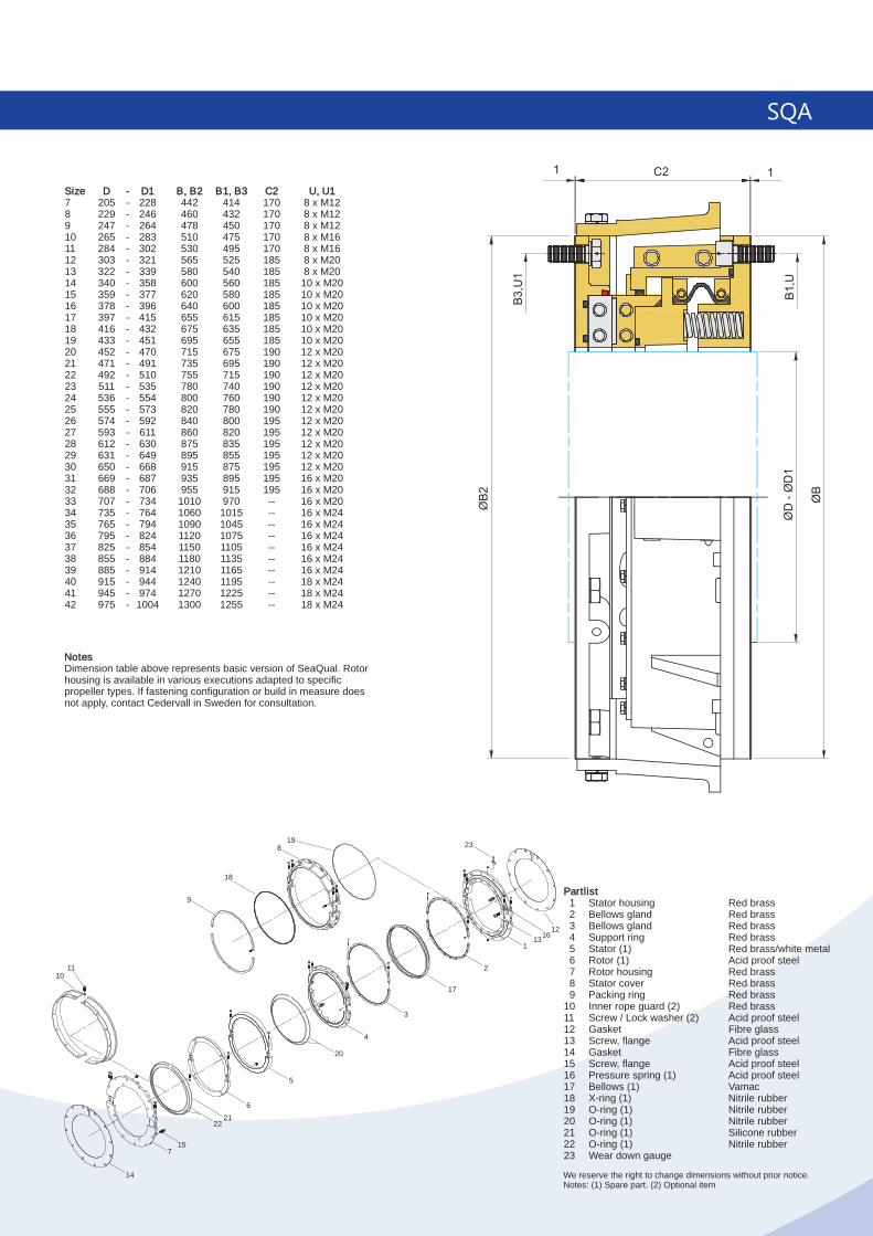
Partlist 1 Stator housing Red brass 2 Bellows gland Red brass 3 Bellows gland Red brass 4 Support ring Red brass 5 Stator (1) Red brass/white metal 6 Rotor (1) Acid proof steel 7 Rotor housing Red brass 8 Stator cover Red brass 9 Packing ring Red brass10 Inner rope guard (2) Red brass11 Screw / Lock washer (2) Acid proof steel12 Gasket Fibre glass13 Screw, flange Acid proof steel14 Gasket Fibre glass15 Screw, flange Acid proof steel16 Pressure spring (1) Acid proof steel17 Bellows (1) Vamac18 X-ring (1) Nitrile rubber19 O-ring (1) Nitrile rubber20 O-ring (1) Nitrile rubber21 O-ring (1) Silicone rubber22 O-ring (1) Nitrile rubber23 Wear down gauge
113
12
2
17
3
4
20
5
6
2122
7
14
15
10
9
18
8 2319
16
11
NotesDimension table above represents basic version of SeaQual. Rotor housing is available in various executions adapted to specific propeller types. If fastening configuration or build in measure does not apply, contact Cedervall in Sweden for consultation.
SQA
We reserve the right to change dimensions without prior notice.Notes: (1) Spare part. (2) Optional item
Size D - D1 B, B2 B1, B3 C2 U, U17 205 - 228 442 414 170 8 x M128 229 - 246 460 432 170 8 x M129 247 - 264 478 450 170 8 x M1210 265 - 283 510 475 170 8 x M1611 284 - 302 530 495 170 8 x M1612 303 - 321 565 525 185 8 x M2013 322 - 339 580 540 185 8 x M2014 340 - 358 600 560 185 10 x M2015 359 - 377 620 580 185 10 x M2016 378 - 396 640 600 185 10 x M2017 397 - 415 655 615 185 10 x M2018 416 - 432 675 635 185 10 x M2019 433 - 451 695 655 185 10 x M2020 452 - 470 715 675 190 12 x M2021 471 - 491 735 695 190 12 x M2022 492 - 510 755 715 190 12 x M2023 511 - 535 780 740 190 12 x M2024 536 - 554 800 760 190 12 x M2025 555 - 573 820 780 190 12 x M2026 574 - 592 840 800 195 12 x M2027 593 - 611 860 820 195 12 x M2028 612 - 630 875 835 195 12 x M2029 631 - 649 895 855 195 12 x M2030 650 - 668 915 875 195 12 x M2031 669 - 687 935 895 195 16 x M2032 688 - 706 955 915 195 16 x M2033 707 - 734 1010 970 -- 16 x M2034 735 - 764 1060 1015 -- 16 x M2435 765 - 794 1090 1045 -- 16 x M2436 795 - 824 1120 1075 -- 16 x M2437 825 - 854 1150 1105 -- 16 x M2438 855 - 884 1180 1135 -- 16 x M2439 885 - 914 1210 1165 -- 16 x M2440 915 - 944 1240 1195 -- 18 x M2441 945 - 974 1270 1225 -- 18 x M2442 975 - 1004 1300 1255 -- 18 x M24
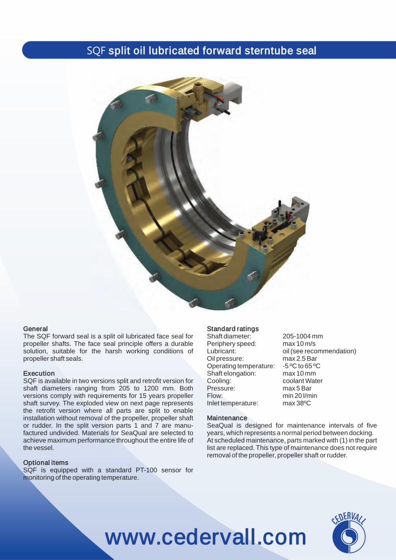
www.cedervall.com
SQF split oil lubricated forward sterntube seal
GeneralThe SQF forward seal is a split oil lubricated face seal forpropeller shafts. The face seal principle offers a durablesolution, suitable for the harsh working conditions ofpropeller shaft seals.
ExecutionSQF is available in two versions split and retrofit version forshaft diameters ranging from 205 to 1200 mm. Bothversions comply with requirements for 15 years propellershaft survey. The exploded view on next page representsthe retrofit version where all parts are split to enableinstallation without removal of the propeller, propeller shaftor rudder. In the split version parts 1 and 7 are manu-factured undivided. Materials for SeaQual are selected toachieve maximum performance throughout the entire life ofthe vessel.
Optional itemsSQF is equipped with a standard PT-100 sensor formonitoring of the operating temperature.
Standard ratingsShaft diameter: 205-1004 mmPeriphery speed: max 10 m/sLubricant: oil (see recommendation)Oil pressure: max 2.5 BarOperating temperature: -5 ºC to 65 ºCShaft elongation: max 10 mmCooling: coolant WaterPressure: max 5 BarFlow: min 20 l/minInlet temperature: max 38ºC
MaintenanceSeaQual is designed for maintenance intervals of fiveyears, which represents a normal period between docking.At scheduled maintenance, parts marked with (1) in the partlist are replaced. This type of maintenance does not requireremoval of the propeller, propeller shaft or rudder.
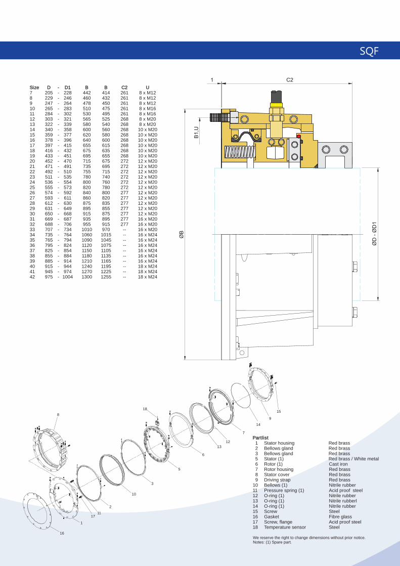
Partlist 1 Stator housing Red brass 2 Bellows gland Red brass 3 Bellows gland Red brass 5 Stator (1) Red brass / White metal 6 Rotor (1) Cast iron 7 Rotor housing Red brass 8 Stator cover Red brass 9 Driving strap Red brass10 Bellows (1) Nitrile rubber11 Pressure spring (1) Acid proof steel12 O-ring (1) Nitrile rubber13 O-ring (1) Nitrile rubberl14 O-ring (1) Nitrile rubber15 Screw Steel16 Gasket Fibre glass17 Screw, flange Acid proof steel18 Temperature sensor Steel
14
13
7
6
5
18
3
10
211
12
8
1
16
17
9
15
SQF
We reserve the right to change dimensions without prior notice.Notes: (1) Spare part.
Size D - D1 B B C2 U7 205 - 228 442 414 261 8 x M128 229 - 246 460 432 261 8 x M129 247 - 264 478 450 261 8 x M1210 265 - 283 510 475 261 8 x M1611 284 - 302 530 495 261 8 x M1612 303 - 321 565 525 268 8 x M2013 322 - 339 580 540 268 8 x M2014 340 - 358 600 560 268 10 x M2015 359 - 377 620 580 268 10 x M2016 378 - 396 640 600 268 10 x M2017 397 - 415 655 615 268 10 x M2018 416 - 432 675 635 268 10 x M2019 433 - 451 695 655 268 10 x M2020 452 - 470 715 675 272 12 x M2021 471 - 491 735 695 272 12 x M2022 492 - 510 755 715 272 12 x M2023 511 - 535 780 740 272 12 x M2024 536 - 554 800 760 272 12 x M2025 555 - 573 820 780 272 12 x M2026 574 - 592 840 800 277 12 x M2027 593 - 611 860 820 277 12 x M2028 612 - 630 875 835 277 12 x M2029 631 - 649 895 855 277 12 x M2030 650 - 668 915 875 277 12 x M2031 669 - 687 935 895 277 16 x M2032 688 - 706 955 915 277 16 x M2033 707 - 734 1010 970 -- 16 x M2034 735 - 764 1060 1015 -- 16 x M2435 765 - 794 1090 1045 -- 16 x M2436 795 - 824 1120 1075 -- 16 x M2437 825 - 854 1150 1105 -- 16 x M2438 855 - 884 1180 1135 -- 16 x M2439 885 - 914 1210 1165 -- 16 x M2440 915 - 944 1240 1195 -- 18 x M2441 945 - 974 1270 1225 -- 18 x M2442 975 - 1004 1300 1255 -- 18 x M24

Where bulkhead openings for
shafts have to be sealed to pro-
tect adjoining spaces against
flooding, the Centrax bulkhead
seal offers the optimum solution.
An axially split housing made of
aluminium is mounted on the
bulkhead opening.
Two garter springs and a seg-
mented thrust ring ensure
proper contact of the sealing
faces on the shaft and on the
housing sides.
Radial and axial shaft move-
ments are taken up by the Cen-
trax bulkhead seal without any
problem. There is practically no
wear owing to the very good
self-lubricating property of the
carbon rings. Aside from the
standard design shown, special
designs with greater radial and/or
angular movement are available.
The Centrax bulkhead seal is
a well proven product, in ser-
vice with merchant and naval
shipping.
46 CENTRAXSeal for Bulkhead Openings
Size Shaft-øD D1 D2 D3 E L L1 L2
60 50- 60 130 175 200
70 61- 70 140 185 210
80 71- 80 150 195 220 8 x M8 62 13
90 81- 90 160 205 230
100 91-100 170 215 240
120 101 - 120 210 262 290
140 121 - 140 230 282 310
160 141 - 160 250 302 330 8 x M12 65 6 15
180 161 - 180 270 322 350
200 181 - 200 290 342 370
220 201 - 220 325 390 430
240 221 - 240 345 410 450
260 241 - 260 365 430 470
280 261 - 280 385 450 490 12 x M16 79 20
300 281 - 300 405 470 510
320 301 - 320 425 490 530
340 321 - 340 445 510 550
360 341 - 360 480 560 610
380 361 - 380 500 580 630
400 381 - 400 520 600 650
420 401 - 420 540 620 670 12 x M20 86 23
440 421 - 440 560 640 690
460 441 - 460 580 660 710
480 461 - 480 600 680 730
500 481 - 500 620 700 750
520 501 - 520 640 725 775
540 521 - 540 660 745 795
560 541 - 560 680 765 815
580 561 - 580 700 785 835 16 x M20 93 8 27
600 581 - 600 720 805 855
620 601 - 620 740 825 875
640 621 - 640 760 845 895
660 641 - 660 790 885 945
680 661 - 680 810 905 965
700 681 - 700 830 925 985
720 701 - 720 850 945 1005
740 721 - 740 870 965 1025 16 x M24 103 33
760 741 - 760 890 985 1045
780 761 - 780 910 1005 1065
800 781 - 800 930 1025 1085

segmentos final 2.dtb.txt
DT BEAM version 1.0 ********************************************************************** Datos Obtenidos con el sofware ********************************************************************** Comments: ========= cargas por segmentos con unidades de elasticidad y densidad corregidas el apoyo de la helice esta a 1/3 del cojinete Units: ====== System = User Defined Length = mm Force = kN Deflection = mm Rotation = rad Span Properties: ================ Length = [mm] Area = [mm^2] Inertia = [mm^4] Elasticity = [kN/mm^2] Density = [kN/mm^3] Number of beam spans = 6 Span Length Area Inertia Elasticity Density 1 674 109955.74 2256841622.5 206 0.0000000785 2 8926 98017.69 1825579491.0 206 0.0000000785 3 6520 98017.69 1825579491.0 206 0.0000000785 880 273240.02 12709076478. 206 0.0000000785 1000 98017.69 1825579491.0 206 0.0000000785 4 7265 98017.69 1825579491.0 206 0.0000000785 5 1000 70921.45 1015063312.5 206 0.0000000785 770 202868.35 7163788454.2 206 0.0000000785 3665 70921.45 1015063312.5 206 0.0000000785 6 6699 70921.45 1015063312.5 206 0.0000000785 Support Properties: =================== kx = ky = [kN/mm] kz = [kN*mm/rad] Rotation = [rad] Sup Type Fix Kx Ky Kz Rotation 1 Free 2 Pinned xy 3 Pinned xy 4 Pinned xy
Página 1

segmentos final 2.dtb.txt 5 Pinned xy 6 Pinned xy 7 Fixed xyz Apply span self weight to the following spans: ============================================== All spans Concentrated Point Loads on Spans: ================================== P = [kN] or [kN*mm] a = [mm] Span P a Dir 1 71 0 -Y ********************************************************************** RESULTS OF ANALYSIS ********************************************************************** Force = [kN] or [kN*mm] Displacement = [mm] or [rad] Location = [mm]
SUPPORT JOINT REACTIONS (in direction of rotated joint axes) =================================================================== JOINT X-REACTION Y-REACTION Z-MOMENT 1 0.00000 0.00000 0.00000 2 0.00000 110.91106 0.00000 3 0.00000 69.50400 0.00000 4 0.00000 73.28191 0.00000 5 0.00000 46.35127 0.00000 6 0.00000 34.22748 0.00000 7 0.00000 19.38856 -22474.40501
MEMBER INTERNAL FORCES (at even intervals along span length) =================================================================== SPAN 1 AXIAL SHEAR MOMENT 0 0.00000 0.00000 0.00000 1 0.00000 -71.58176 -4805.00547 2 0.00000 -72.16353 -9649.22190 3 0.00000 -72.74529 -14532.64927 4 0.00000 -73.32706 -19455.28759
Página 2
segmentos final 2.dtb.txt 5 0.00000 -73.90882 -24417.13686 6 0.00000 -74.49059 -29418.19709 7 0.00000 -75.07235 -34458.46826 8 0.00000 -75.65412 -39537.95037 9 0.00000 -76.23588 -44656.64344 10 0.00000 -76.81765 -49814.54746 SPAN 2 0 0.00000 34.09341 -49814.54746 1 0.00000 27.22540 -22447.96484 2 0.00000 20.35739 -1211.76913 3 0.00000 13.48937 13894.03967 4 0.00000 6.62136 22869.46156 5 0.00000 -0.24665 25714.49656 6 0.00000 -7.11466 22429.14464 7 0.00000 -13.98267 13013.40582 8 0.00000 -20.85068 -2532.71991 9 0.00000 -27.71869 -24209.23255 10 0.00000 -34.58671 -52016.13209 SPAN 3 0 0.00000 34.91729 -52016.13209 1 0.00000 28.45401 -25400.18492 2 0.00000 21.99072 -4213.39839 3 0.00000 15.52744 11544.22749 4 0.00000 9.06415 21872.69273 5 0.00000 2.60086 26771.99734 6 0.00000 -3.86242 26242.14129 7 0.00000 -10.32571 20283.12461 8 0.00000 -19.53999 8619.84823 9 0.00000 -35.35664 -15185.00582 10 0.00000 -41.81993 -47599.16561 SPAN 4 0 0.00000 31.46198 -47599.16561 1 0.00000 25.87201 -26772.59524 2 0.00000 20.28203 -10007.14052 3 0.00000 14.69206 2697.19855 4 0.00000 9.10209
Página 3
segmentos final 2.dtb.txt11340.42197 5 0.00000 3.51211 15922.52974 6 0.00000 -2.07786 16443.52186 7 0.00000 -7.66783 12903.39833 8 0.00000 -13.25781 5302.15915 9 0.00000 -18.84778 -6360.19568 10 0.00000 -24.43775 -22083.66616 SPAN 5 0 0.00000 21.91352 -22083.66616 1 0.00000 18.88767 -10995.94151 2 0.00000 14.96070 -1591.96335 3 0.00000 6.30537 4187.09028 4 0.00000 1.83461 6107.25536 5 0.00000 -1.19124 6282.09019 6 0.00000 -4.21709 4812.37775 7 0.00000 -7.24293 1698.11805 8 0.00000 -10.26878 -3060.68892 9 0.00000 -13.29462 -9464.04316 10 0.00000 -16.32047 -17511.94465 SPAN 6 0 0.00000 17.90701 -17511.94465 1 0.00000 14.17745 -6765.25485 2 0.00000 10.44789 1483.00477 3 0.00000 6.71834 7232.83420 4 0.00000 2.98878 10484.23345 5 0.00000 -0.74078 11237.20251 6 0.00000 -4.47033 9491.74138 7 0.00000 -8.19989 5247.85006 8 0.00000 -11.92945 -1494.47144 9 0.00000 -15.65900 -10735.22313 10 0.00000 -19.38856 -22474.40501
SUPPORT JOINT DISPLACEMENTS (in direction of rotated joint axes) =================================================================== JOINT X-DISPLACEMENT Y-DISPLACEMENT Z-ROTATION 1 0.000000000 -0.011760939
Página 4
segmentos final 2.dtb.txt0.000029249 2 0.000000000 0.000000000 -0.000006386 3 0.000000000 0.000000000 -0.000002323 4 0.000000000 0.000000000 0.000050724 5 0.000000000 0.000000000 0.000031429 6 0.000000000 0.000000000 -0.000026497 7 0.000000000 0.000000000 0.000000000
MEMBER DISPLACEMENTS (at even intervals along span length) =================================================================== SPAN 1 X-DISPLACEMENT Y-DISPLACEMENT Z-ROTATION 0 0.000000000 -0.011760939 0.000029249 1 0.000000000 -0.009797365 0.000028901 2 0.000000000 -0.007880775 0.000027854 3 0.000000000 -0.006058501 0.000026101 4 0.000000000 -0.004378262 0.000023638 5 0.000000000 -0.002888158 0.000020459 6 0.000000000 -0.001636673 0.000016557 7 0.000000000 -0.000672673 0.000011927 8 0.000000000 -0.000045408 0.000006564 9 0.000000000 0.000195488 0.000000461 10 0.000000000 0.000000000 -0.000006386 SPAN 2 0 0.000000000 0.000000000 -0.000006386 1 0.000000000 -0.048264505 -0.000090931 2 0.000000000 -0.145169233 -0.000117797 3 0.000000000 -0.245723508 -0.000101534 4 0.000000000 -0.317924398 -0.000056692 5 0.000000000 -0.342756712 0.000002177 6 0.000000000 -0.314193003 0.000060524 7 0.000000000 -0.239193568 0.000103798 8 0.000000000 -0.137706444 0.000117449 9 0.000000000 -0.042667413 0.000086925 10 0.000000000 0.000000000 -0.000002323 SPAN 3 0 0.000000000 0.000000000 -0.000002323
Página 5
segmentos final 2.dtb.txt 1 0.000000000 -0.042001163 -0.000087772 2 0.000000000 -0.132508283 -0.000119834 3 0.000000000 -0.231769662 -0.000110636 4 0.000000000 -0.310220061 -0.000072305 5 0.000000000 -0.348480701 -0.000016968 6 0.000000000 -0.337359265 0.000043250 7 0.000000000 -0.277849894 0.000096221 8 0.000000000 -0.181637084 0.000125018 9 0.000000000 -0.076701179 0.000119831 10 0.000000000 0.000000000 0.000050724 SPAN 4 0 0.000000000 0.000000000 0.000050724 1 0.000000000 0.008557758 -0.000020459 2 0.000000000 -0.020934002 -0.000055331 3 0.000000000 -0.064945458 -0.000061738 4 0.000000000 -0.105646448 -0.000047526 5 0.000000000 -0.130906462 -0.000020538 6 0.000000000 -0.134294647 0.000011378 7 0.000000000 -0.115079807 0.000040379 8 0.000000000 -0.078230400 0.000058618 9 0.000000000 -0.034414541 0.000058249 10 0.000000000 0.000000000 0.000031429 SPAN 5 0 0.000000000 0.000000000 0.000031429 1 0.000000000 0.004190511 -0.000011205 2 0.000000000 -0.007307584 -0.000026355 3 0.000000000 -0.021558606 -0.000025732 4 0.000000000 -0.033238021 -0.000014509 5 0.000000000 -0.036671875 0.000001949 6 0.000000000 -0.031424848 0.000016723 7 0.000000000 -0.019573150 0.000025540 8 0.000000000 -0.005516182 0.000024126 9 0.000000000 0.004023463 0.000008205 10 0.000000000 0.000000000 -0.000026497 SPAN 6 0 0.000000000 0.000000000
Página 6
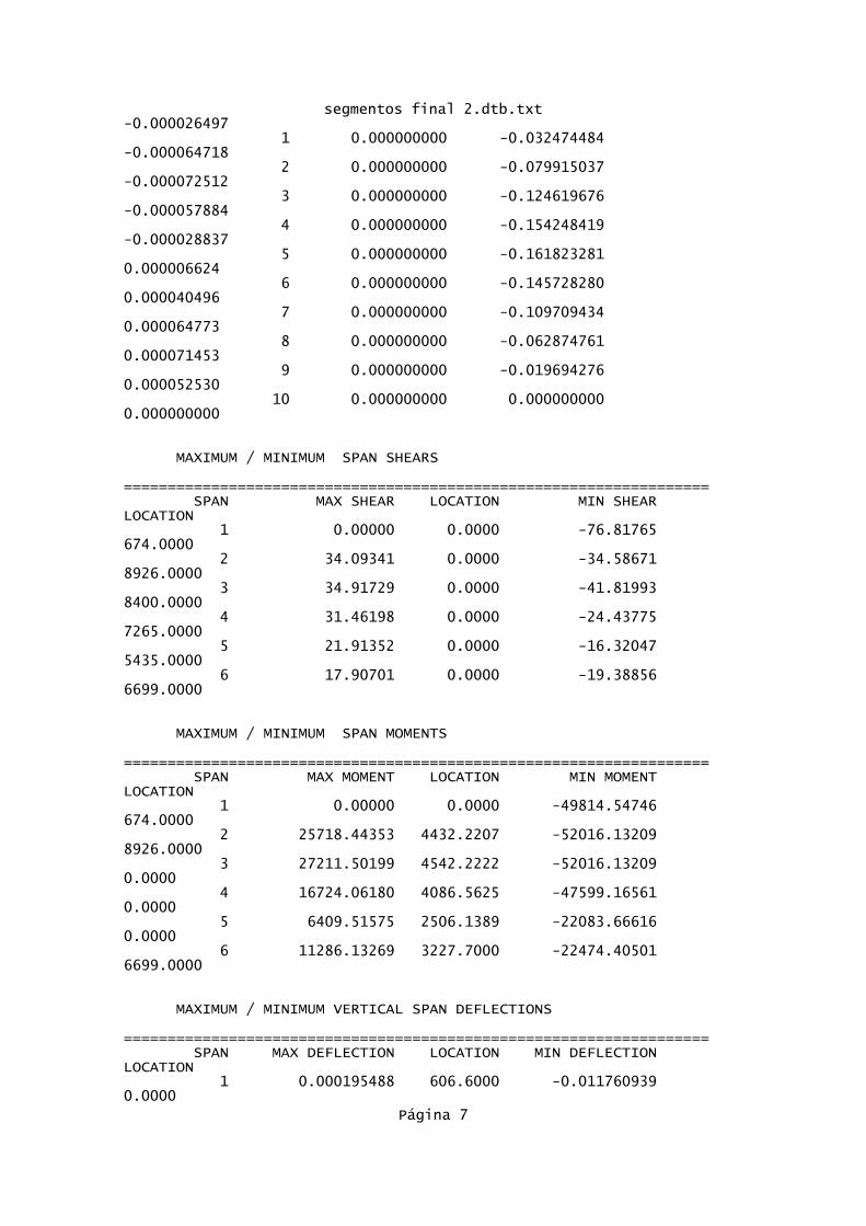
segmentos final 2.dtb.txt-0.000026497 1 0.000000000 -0.032474484 -0.000064718 2 0.000000000 -0.079915037 -0.000072512 3 0.000000000 -0.124619676 -0.000057884 4 0.000000000 -0.154248419 -0.000028837 5 0.000000000 -0.161823281 0.000006624 6 0.000000000 -0.145728280 0.000040496 7 0.000000000 -0.109709434 0.000064773 8 0.000000000 -0.062874761 0.000071453 9 0.000000000 -0.019694276 0.000052530 10 0.000000000 0.000000000 0.000000000
MAXIMUM / MINIMUM SPAN SHEARS =================================================================== SPAN MAX SHEAR LOCATION MIN SHEAR LOCATION 1 0.00000 0.0000 -76.81765 674.0000 2 34.09341 0.0000 -34.58671 8926.0000 3 34.91729 0.0000 -41.81993 8400.0000 4 31.46198 0.0000 -24.43775 7265.0000 5 21.91352 0.0000 -16.32047 5435.0000 6 17.90701 0.0000 -19.38856 6699.0000
MAXIMUM / MINIMUM SPAN MOMENTS =================================================================== SPAN MAX MOMENT LOCATION MIN MOMENT LOCATION 1 0.00000 0.0000 -49814.54746 674.0000 2 25718.44353 4432.2207 -52016.13209 8926.0000 3 27211.50199 4542.2222 -52016.13209 0.0000 4 16724.06180 4086.5625 -47599.16561 0.0000 5 6409.51575 2506.1389 -22083.66616 0.0000 6 11286.13269 3227.7000 -22474.40501 6699.0000
MAXIMUM / MINIMUM VERTICAL SPAN DEFLECTIONS =================================================================== SPAN MAX DEFLECTION LOCATION MIN DEFLECTION LOCATION 1 0.000195488 606.6000 -0.011760939 0.0000
Página 7
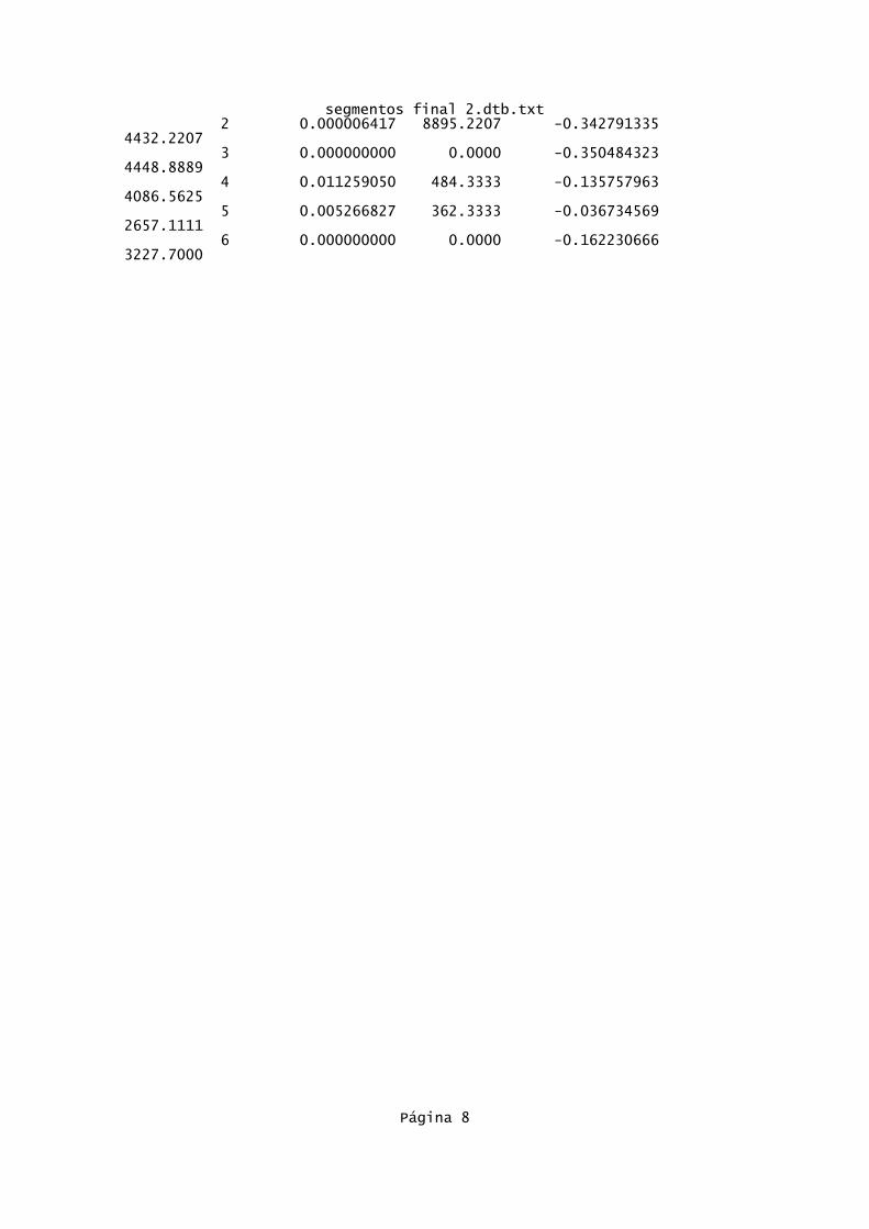
segmentos final 2.dtb.txt 2 0.000006417 8895.2207 -0.342791335 4432.2207 3 0.000000000 0.0000 -0.350484323 4448.8889 4 0.011259050 484.3333 -0.135757963 4086.5625 5 0.005266827 362.3333 -0.036734569 2657.1111 6 0.000000000 0.0000 -0.162230666 3227.7000
Página 8