projecte o tesina d’especialitat - pàgina inicial de ... · projecte o tesina d’especialitat...
TRANSCRIPT

PROJECTE O TESINA D’ESPECIALITAT
Títol
Analysis of the performance of SWASH in harbour domains
Autor/a
Joan Alabart Llinàs
Tutor/a
Agustín Sánchez-Arcilla Conejo
Gerbrant Van Vledder
Departament
Enginyeria Hidràulica, Marítima i Ambiental
Intensificació
Enginyeria Marítima
Data
Octubre 2013

ANALYSIS OF THE PERFORMANCE
OF SWASH IN HARBOUR DOMAINS
Treball Final de Carrera - Tesina
Enginyeria de Camins, Canals i Ports
Octubre 2013
Autor: Joan Alabart Llinàs
Tutors: Agustín Sánchez-Arcilla Conejo
Gerbrant Van Vledder
Technische Universiteit Delft
Faculteit Civiele Techniek en
Geowetenschappen
Department of Fluid Mechanics
Universitat Politècnica de Catalunya
Escola Tècnica Superior d’Enginyers de
Camins, Canals i Ports de Barcelona
Departament d’Enginyeria Hidràulica,
Marítima i Ambiental

Joan Alabart Llinàs 3
ABSTRACT PRESENTED IN THE 3RD IAHR EUROPE CONGRESS, 2014 IN
PORTO
ANALYSIS OF THE PERFORMANCE OF SWASH IN HARBOUR DOMAINS
JOAN ALABART(1), AGUSTÍN SÁNCHEZ-ARCILLA(2) & GERBRANT VAN VLEDDER(3)
(1) ETSECCPB and TU DELFT, [email protected] (2) [email protected] (3) [email protected]
Wave penetration inside harbours has been one the main issues that port planners and engineers have had to deal with in recent years. Wave conditions inside harbours trigger vessel movements, create dynamic loads on port structures and condition harbour exploitation and safety. For this reason in the recent past maritime and port engineers have developed a set of semi-empirical criteria and physical modelling tools to design the layout of breakwaters and other protection structures. Nevertheless, with the development of computers and numerical methods, several models have tried to simulate the propagation of waves inside such restricted domains, affected by multiple competing processes such as diffraction, partial reflection, etc. It is in this framework where SWASH (Simulating WAves till SHore), a model developed by TU Delft, is expected to perform realistic and accurate simulations well beyond the performance limits of other state of the art codes.
SWASH solves directly the momentum conservation laws and can deal with dyke geometry and even porosity. It is very suited for simulating non-hydrostatic, free-surface flows, including long-wave generation and short wave propagation. Because of that we shall here evaluate how such a model can simulate the propagation of various types of waves in real harbour cases. The Port of Blanes, located in the Catalan coast with wave measurements available, was chosen as our test case. The wave climate recorded offshore the harbour entrance was introduced as model boundary condition, together with features of the harbour structures. The output from the model was then compared to the actual measurements inside the Port.
The results show that SWASH can be indeed a rather useful tool for harbour engineering, providing realistic and accurate results. Furthermore, the way the model accounts for porous structures can be considered to be quite flexible and realistic.
Finally some conclusions and recommendations for further work in this topic have been drawn and will be presented in the paper. This will set the basis for further development of this numerical tool that could become the cornerstone of port layout planning in the coming years.
Figure. Layout of the Blanes
harbour in the Spanish
Mediterranean coast showing
the HRMS wave map during
storm conditions and the
main measurement point
inside the port domain that
has been used for the
assessment of the model
performance.
X coordinate (m)
Y c
oord
inat
e (m
)
Port of Blanes, HRMS map
4.828 4.829 4.83 4.831 4.832 4.833 4.834 4.835 4.836 4.837 4.838
x 105
4.6133
4.6134
4.6135
4.6136
4.6137
4.6138
4.6139
4.614
4.6141
x 106 HRMS (m)
0
0.5
1
1.5
Buoy Port
Joan Alabart Llinàs 4
SUMMARY
TITLE: ANALYSIS OF THE PERFORMANCE OF SWASH IN HARBOUR DOMAINS
AUTHOR: JOAN ALABART LLINAS
SUPERVISORS: AGUSTÍN SÁNCHEZ-ARCILLA CONEJO / GERBRANT VAN VLEDDER
Wave penetration inside harbours has been one the main issues that port planners and engineers have had to deal with in recent years. Wave conditions inside harbours trigger vessel movements; create dynamic loads on port structures and condition harbour exploitation and safety. For this reason in the recent past maritime and port engineers have developed a set of semi-empirical criteria and physical modelling tools to design the layout of breakwaters and other protection structures. Nevertheless, with the development of computers and numerical methods, several models have tried to simulate the propagation of waves inside such restricted domains, affected by multiple competing processes such as diffraction, partial reflection, etc. It is in this framework where SWASH (Simulating WAves till SHore), a model developed by TU Delft, is expected to perform realistic and accurate simulations well beyond the performance limits of other state of the art codes.
SWASH solves directly the momentum conservation laws and can deal with dyke geometry and even porosity. It is very suited for simulating non-hydrostatic, free-surface flows, including long-wave generation and short wave propagation. Because of that we shall here evaluate how such a model can simulate the propagation of various types of waves in real harbour cases. The Port of Blanes, located in the Catalan coast with wave measurements available, was chosen as our test case.
Previous to the performance of the simulation of the case study, several 1D and 2D simulations were undergone to get acquaint with the model. Furthermore, an exhaustive analysis of the response of SWASH when using porous layers was included. The reason for it was double. On the one hand, to see how the model accounted for porous layers such as dykes and breakwaters. On the other hand, to try to solve the stability problems that the inclusion of those layers may produce. A certain setting when it comes to the numerical discretization of the equations was found to be stable and provide reliable results and used afterwards in the case study of the Port of Blanes.
To perform the simulation of the Port of Blanes real case, initially a wave approach with SWAN was performed as the wave data was too far from the entrance of the port. To do so the bathymetry of the surroundings of the port was needed. The output of these simulations was inputted later on in SWASH to do the final stage of the simulation within the port. To do the simulation, an accurate bathymetry of the actual port during the year were the measurements were done was necessary, and a data treatment was done to include the new structures to the out of date bathymetry that could be provided.
These simulations accounted for the port structures as porous layers that emulated the partial reflection and transmission phenomena, diffraction and refraction that are present in port domains. The output from the model was then compared to the actual measurements inside the port and a comparison was made.
The results show that SWASH can be indeed a rather useful tool for harbour engineering, providing realistic and accurate results. Furthermore, the way the model accounts for porous structures can be considered to be quite flexible and realistic.
Finally some conclusions and recommendations for further work in this topic have been drawn. This will set the basis for further development of this numerical tool that could become the cornerstone of port layout planning in the coming years.

Joan Alabart Llinàs 5
RESUMEN
TÍTULO: ANALYSIS OF THE PERFORMANCE OF SWASH IN HARBOUR DOMAINS
AUTOR: JOAN ALABART LLINAS
TUTORES: AGUSTÍN SÁNCHEZ-ARCILLA CONEJO / GERBRANT VAN VLEDDER
La penetración de oleaje en puertos ha sido uno de los principales problemas que los planificadores de puertos e ingenieros han tenido que solucionar en los últimos años. Las condiciones de oleaje en puertos inducen movimientos en las embarcaciones, crean cargas dinámicas en las estructuras portuarias y condicionan la seguridad de la explotación portuaria. Por esta razón en el pasado reciente, los ingenieros marítimos y portuarios desarrollaron un séquito de criterios semiempíricos y reglas de modelización para diseñar las estructuras de protección. Sin embargo, con el desarrollo de los ordenadores y los métodos numéricos, diversos modelos han intentado simular la propagación del oleaje en estos dominios restrictivos afectados por múltiples procesos superpuestos tales como difracción, reflexión parcial, etc. Es en este marco donde SWASH (Simulating WAves till SHore), modelo desarrollado en TU Delft, se prevé que será capaz de realizar simulaciones mucho más realistas y precisas que otros modelos actualmente disponibles.
SWASH resuelve directamente las ecuaciones de conservación del momento y puede incorporar la geometría de los diques y su porosidad. Es idóneo para simular flujos no-hidrostáticos, con superficie libre, incluyendo la generación de olas largas y propagación de olas cortas. Por eso debemos evaluar cómo este modelo puede simular varios tipos de oleaje en puertos reales. El Puerto de Blanes, localizado en la costa catalana que tiene mediciones disponibles, fue elegido como caso de estudio.
Previo a la realización de las simulaciones del caso de estudio, diversas simulaciones en 1D y 2D se realizaron para familiarizarse con el modelo. Además se realizó un análisis exhaustivo de la respuesta de SWASH ante la inclusión de capas porosas. La primera razón fue para ver como el modelo tomaba en cuenta las capas porosas tales como diques y rompeolas; la segunda razón para solucionar los problemas de inestabilidad derivados de la inclusión de dichas capas. Con ello se encontró una cierta discretización numérica de las ecuaciones que era estable y proporcionaba resultados realistas y que fue usada en el caso del Puerto de Blanes.
Para realizar la simulación del Puerto de Blanes, inicialmente se propagó el oleaje con SWAN hacia la costa ya que la boya de la que se disponían datos estaba demasiado lejos de la entrada del puerto. Para ello se necesitó la batimetría de los alrededores del puerto. Los resultados de estas simulaciones se pusieron como datos de partida en SWASH para realizar la última fase de la propagación. Para realizar estas simulaciones, una batimetría precisa del puerto durante el año donde se tomaron las medidas era necesaria por lo que un tratamiento de los datos fue realizado para incluir las estructuras portuarias nuevas a la batimetría disponible que no estaba actualizada.
Estas simulaciones tuvieron en cuenta las estructuras portuarias como capas porosas que emulaban la reflexión y transmisión parciales, la difracción y la refracción que son presentes en estos dominios. Los resultados del modelo se compararon con las mediciones reales dentro del puerto.
Los resultados muestran que SWASH es una herramienta muy útil para la ingeniería portuaria ya que da resultados realistas y precisos. Además, la forma como incluye las capas porosas es flexible y realista.
Finalmente se aportaron conclusiones y recomendaciones para futuros trabajos estableciendo las bases para futuros desarrollos de esta herramienta numérica que podría convertirse en la piedra angular del planeamiento portuario en los años venideros.

Joan Alabart Llinàs 6
ACKNOWLEDGEMENTS
First of all, I would like to thank my supervisor from the UPC Prof. Agustín Sánchez-Arcilla Conejo because he was the one that suggested this topic for the thesis, provided relevant information and acted as the link between the UPC and TU Delft.
Secondly, I would also like to thank my supervisor from TU Delft Prof. Gerbrant Van Vledder because he was the main responsible of the success of this thesis guiding my through it, providing essential information and knowledge and giving me the chance to contact people alien to the university that were interested on this topic.
I would also like to thank Prof. Marcel Zijlema because he helped me to become acquaint with SWASH and provided useful information to solve the issues I encountered.
I would also like to mention and thank the interest of the company Witteveen Bos to collaborate in this project.
Ultimately, I would like to thank my fellow exchange students Víctor Martínez Pes with whom I had interesting discussions about SWASH, and Víctor Chavarrías Borrás for being always the person with whom I have learned more and whose help has been priceless during all my studies.
At last I want to thank my parents for giving their unconditional support during all my studies no matter how things went.
Joan Alabart Llinàs
Delft, June 2013
Joan Alabart Llinàs 7
TABLE OF CONTENTS
CHAPTER 1: GENERAL INFORMATION .................................................................................... 11
1.1. INTRODUCTION ........................................................................................................... 11
1.2. OBJECTIVES .................................................................................................................. 12
1.3. PROBLEM APPROACH .................................................................................................. 12
1.4. RELEVANCE OF THE STUDY.......................................................................................... 13
CHAPTER 2: BACKGROUND KNOWLEDGE .............................................................................. 14
2.1. SURFACE GRAVITY WAVES .......................................................................................... 14
2.2. LINEAR WAVE THEORY ................................................................................................ 15
2.3. PROPAGATION OF WAVES .......................................................................................... 18
2.3.1. SHOALING ................................................................................................................ 19
2.3.2. REFRACTION ............................................................................................................ 20
2.3.3. REFLECTION AND TRANSMISSION ........................................................................... 22
2.3.4. DIFFRACTION ........................................................................................................... 23
2.3.5. WAVE BREAKING ..................................................................................................... 25
2.3.6. NON-LINEAR EFFECTS .............................................................................................. 26
2.4. WAVE ANALYSIS .......................................................................................................... 28
2.4.1. RAYLEIGH DISTRIBUTION ......................................................................................... 28
2.4.2. SPECTRAL ANALYSIS ................................................................................................ 29
2.4.3. DIRECTIONAL SPECTRUM ........................................................................................ 31
2.4.4. IDEALIZED SPECTRA ................................................................................................. 32
CHAPTER 3: WAVE PROPAGATION MODELLING.................................................................... 33
3.1. BACKGROUND ............................................................................................................. 33
3.2. MODELS AVAILABLE .................................................................................................... 34
3.3. PHASE AVERAGED AND PHASE SOLVING MODELS ..................................................... 35
3.4. SWASH ......................................................................................................................... 36
CHAPTER 4: POROUS STRUCTURES ........................................................................................ 40
4.1. INTRODUCTION ........................................................................................................... 40
4.2. BACKGROUND ON POROUS STRUCTURES .................................................................. 40
4.3. POROSITY IN SWASH ................................................................................................... 42
4.4. SIMPLIFIED 1D CASES ANALYSIS .................................................................................. 43
4.5. STABILITY OF THE SIMULATION WITH POROUS STRUCTURES .................................... 46
Joan Alabart Llinàs 8
CHAPTER 5: REAL CASE OF THE PORT OF BLANES ................................................................. 51
5.1. INTRODUCTION ........................................................................................................... 51
5.2. WAVE CLIMATE ........................................................................................................... 52
5.2.1. NORMAL WAVE CLIMATE ANALYSIS ....................................................................... 52
5.2.2. EXTREME WAVE CLIMATE ANALYSIS ....................................................................... 54
5.2.3. NORMAL WAVE CLIMATE REGISTER YEAR 2011 ..................................................... 55
5.2.4. EXTREME WAVE CLIMATE ANALYSIS YEAR 2011 .................................................... 58
5.3. BATHYMETRY ADAPTATION AND PREPARATION ........................................................ 59
5.4. SWAN WAVE APPROACH ............................................................................................ 63
5.5. SWASH WAVE PROPAGATION WITHIN THE PORT ...................................................... 65
5.6. COMPARISON OF THE RESULTS WITH THE MEASUREMENTS ..................................... 70
CHAPTER 6: CONCLUSIONS AND RECOMMENDATIONS ........................................................ 74
6.1. CONCLUSIONS ............................................................................................................. 74
6.2. RECOMMENDATIONS .................................................................................................. 74
CHAPTER 7: REFERENCES ........................................................................................................ 77
ANNEX 1 ……………………………………………………………………………………..………………………………..……….79
ANNEX 2 ……………………………………………………………………………………..………………………………..……….91
ANNEX 3 ……………………………………………………………………………………..………………………………..…….103

Joan Alabart Llinàs 9
LIST OF FIGURES
Figure 1. Surface gravity waves classification (Kinsman, 1984). ................................................................ 14
Figure 2. Orbital motion representation (Wikipedia). ................................................................................ 17
Figure 3. Shoaling scheme Source: The COMET Program. .......................................................................... 19
Figure 4. Shoaling coefficient variation with dimensionless depth (Fenton, 2010). ................................... 20
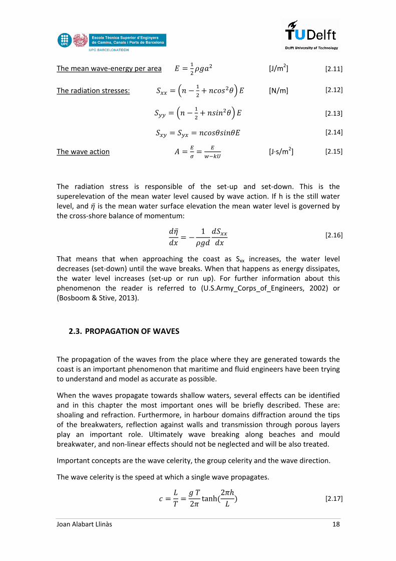
Figure 5. Refraction scheme Source: The COMET Program. ....................................................................... 21
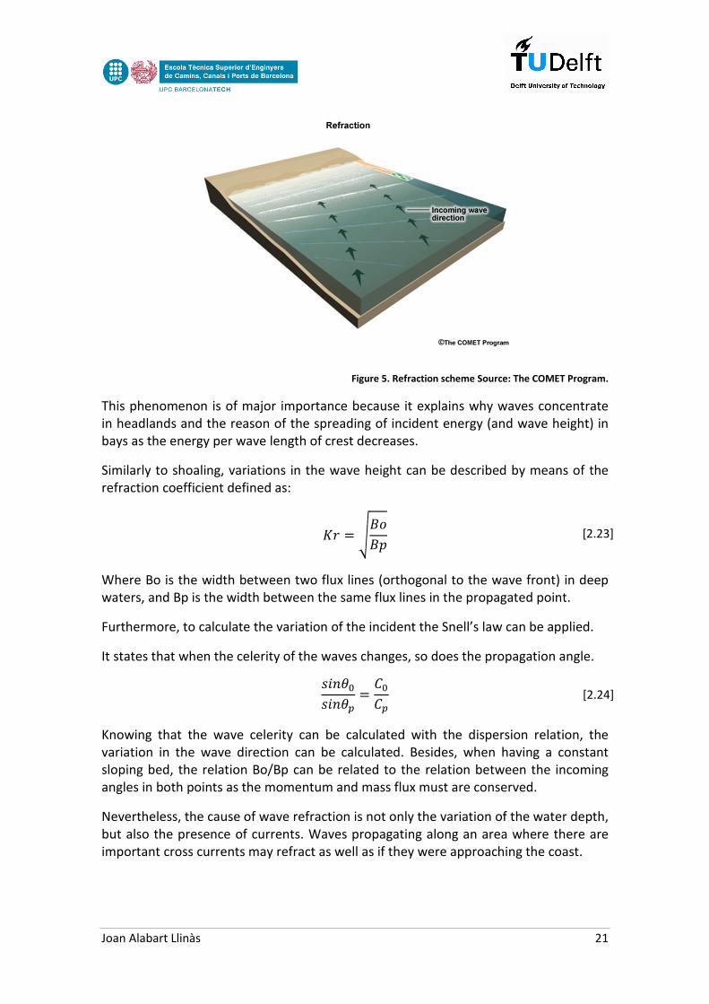
Figure 6. Combination of wave reflection and refraction scheme (Anthoni, 2000). ................................... 22
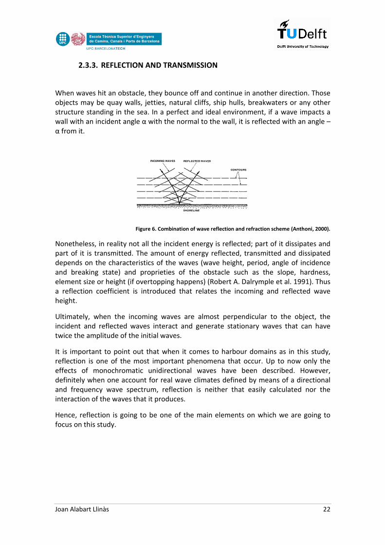
Figure 7. Diffraction scheme around a breakwater (R.Boshek, 2009). ....................................................... 23
Figure 8. Sketch for Sommerfeld Solution (Daemrich & Kohlhase, 2011) ................................................... 24
Figure 9. Wave skewness sketch. Source Coastal Dynamics I slights. ........................................................ 26
Figure 10. Wave asymmetry sketch as a sum of two harmonics dephased. Source Coastal Dynamics I
slights. ........................................................................................................................................................ 27
Figure 11. HRMS map for n=0 (left) and n=0.1 (right). ............................................................................... 44
Figure 12. HRMS map for n=0.5 (left) and n=0.7 (right). ............................................................................ 44
Figure 13. Evolution of T and R for a wave of T=10s, Hs=0.05m, θ=90º, h=10m, d50=0.025m. .................. 45
Figure 14. Evolution of T and R for a wave of T=10s, Hs=0.05m, θ=90º, h=10m, P=0.5............................. 45
Figure 15. Simulation with dx=4m and a structure of 4m width. ............................................................... 46
Figure 16. Simulation A with dx=4 (above) and dx=2m (below). ................................................................ 47
Figure 17. Simulation A with sloping side structure. Dx=4m. Monochromatic waves. ............................... 48
Figure 18. Simulation B. Regular waves (above) and irregular waves (below). ......................................... 48
Figure 19. Modified A simulation with new setting and height structures of 99m. ................................... 50
Figure 20. Plan view of the Port of Blanes during year 2013. Source Google Earth. .................................. 51
Figure 21. Location of the buoy (Buoy Argoss). Source Google Maps. ....................................................... 52
Figure 22. Wave rose 20year record. Source Argoss database. ................................................................. 53
Figure 23. Hm0 density distribution. Source Argoss database. .................................................................. 53
Figure 24. Extract from ROM 03.91 page 34. ............................................................................................. 54
Figure 25. Extreme wave climate linear regression. ................................................................................... 55
Figure 26. Location of the buoy with the records of year 2011. 41º 38.81’N - 2º 48.93’ E......................... 56
Figure 27. Wave rose of the data of year 2011. Source Generalitat de Catalunya database. ................... 56
Figure 28. Hs during the year 2011. Source Generalitat de Catalunya database ....................................... 57
Figure 29. Spectral T-1,1 wave period distribution. Source Generalitat de Catalunya database ................. 57
Figure 30. Extreme wave climate linear regression during year 2011 ........................................................ 58
Figure 31. Wave rose of the storms during 2011 (values in cm). ............................................................... 59
Figure 32. Scatter plot of the data provided from the old bathymetry ...................................................... 60
Figure 33. Plan view of the domain included in the old bathymetry .......................................................... 60
Figure 34. Old bathymetry adapted. The colours indicate the water depth (left). ..................................... 61
Figure 35. New bathymetry adapted from the old one. The colours indicate the water depth (right). ..... 61
Figure 36. Aerial view of the adapted bathymetry ..................................................................................... 61
Figure 37. Bathymetry in the surroundings of Blanes. Source Admiralty Charts database. ....................... 62
Figure 38. Approximated plan view of the simulation grids. SWAN in green and SWASH in yellow. ......... 63
Figure 39. Wind roses near Blanes. January (left) and December (right). Source: Puertos del Estado
database ..................................................................................................................................................... 64
Figure 40. Hsig output map from the simulation of the 16/12/2011 at 13h with SWAN ........................... 65
Figure 41. Simulation of Blanes without porous layers. Structures are bottom variations. ....................... 66
Figure 42. Porosity file. The porosity is n=0.01 for the port structures and 1 in the rest ............................ 67
Figure 43. Smoothed bathymetry using n=1.000.000. ............................................................................... 67

Joan Alabart Llinàs 10
Figure 44. HRMS map from the Port of Blanes. Upper figure with the colours going from 0 to 2m. Lower
figure with the colours going from 0 to 1m for more accuracy within the port. ........................................ 68
Figure 45. Hrms map from the Port of Blanes. Upper figure with the colours going from 0 to 2m. Lower
figure with the colours going from 0 to 1m for more accuracy within the port. ........................................ 69
Figure 46. Location of the buoy inside the port of Blanes in the frame of the old port. Source ICC. .......... 70
LIST OF TABLES
Table 1. Gravity waves, causes and periods (Fenton, 2010). ...................................................................... 15
Table 2. Comparison between SWAN and SWASH. .................................................................................... 36
Table 3. Summary of the 1D cases without changing the discretization settings. ..................................... 49
Table 4. Wave height interpolation for increasing retour periods.............................................................. 55
Table 5. Comparison between the real measurements and the results of the simulation. ........................ 72

Joan Alabart Llinàs 11
CHAPTER 1: GENERAL INFORMATION
1.1. INTRODUCTION
Since the ancient civilizations, harbours have played a major role in the development of society. First of all, their function was only to keep safe the fishing boats that provided a primary food source. Later on, when societies developed, they enabled the diffusion of culture and knowledge by means of commerce and transport. Moreover, until the invention of flight and the improvement of road and rail transport, for many coastal cities, ports represented the only exterior gate.
Nowadays, the function of ports has changed slightly. Via them, goods travel all over the world as it is the cheapest mode of freight transport, and the cleanest in terms of energy efficiency. However, when it comes to passengers, only ferries for short distances and the growing market of leisure cruisers have an important position. Nevertheless, fishing activities are still important even though fishery ports tend to be segregated from commercial ports as the mentality, the requirements and the location are quite different (Ligteringen & Velsink, 2012).
Nonetheless, the layout of actual harbours has not many resemblances to the disposition of the elements in the earlier ports. In our modern society, the design of a port is done according to multiple factors that range from hydraulic and fluid mechanics, to economic analysis, passing through transport chains, logistics, structural design, risk assessment, environmental assessments and many other factors.
Despite this, it must be born in mind that on top of them the goal of the infrastructure is to provide a basin where vessels can operate safely the most time as possible.
That is the reason why maritime engineers have been studying the behaviour of waves, how they propagate towards the coast, which phenomena occur and how those movements affect the transports of sediments along the shore line, the movements and safety of the ships and operations in harbour basins and many other applications.
In order to provide the optimum design of a port, several empirical guidelines are available and have been used until the development of computers. However, at present days with the development of numerical methods, more accurate models try to reproduce the complex reality that those early studies and guides simplified.
Is within this framework where SWASH, the model developed by TU Delft, appears. Before it this university had developed other models like WAVEWATCH III or SWAN which have their own scope of application but failed to reproduce the effects that occur in places with rapidly varying proprieties. Besides, as it is the case in harbour domains where nonlinear theory is mandatory and the effects of diffraction and reflection play a major role, SWASH tried to improve several existing models that could

Joan Alabart Llinàs 12
be applied in the same circumstances developed by universities, companies and other organizations alien to TU Delft.
Thus, SWASH being a more complex model than SWAN (the previous one released by TU Delft), is thought to be able to reproduce satisfactorily the propagation of waves inside ports and hence, become an important tool in port planning and design.
1.2. OBJECTIVES
The main objective of this thesis is to analyse the performance of SWASH in harbour domains by comparing it with real data. Furthermore a compilation of the different available models, their features and drawbacks is also provided by paying special attention to SWASH. Ultimately, it is also a goal of this work to provide some recommendations for further work and the development of further versions of this model.
1.3. PROBLEM APPROACH
To test the behaviour of SWASH inside ports, the Port of Blanes will be used as a real case with the data provided by the UPC.
First of all, some background information will be provided both referring to the theory of wave propagation and modelling. Afterwards some simplified cases will be explained to describe the methodology followed by SWASH to account for the porous structures, the issues that may arise and the best way to cope with them.
Then the real case of the Port of Blanes will be used to check the performance of SWASH and outline the issues that this model still has. To do so, real data outside the port will be used and compared to data collected inside the port. Initially an approximation of the waves to the shoreline will be carried on with SWAN. Then the output will be inputted in SWASH to simulate the wave propagation within the port and the surroundings.
Finally the results of this simulation will be compared to the real measurements and some recommendations for further work in the topic will be drawn.

Joan Alabart Llinàs 13
1.4. RELEVANCE OF THE STUDY
The propagation of waves inside harbours has been studied for a long time and can be treated from two perspectives.
On the one hand we have the physical models that try to emulate the real conditions (or at least the most important features) in a scaled basin or flume. Nonetheless, the drawbacks that this methodology has are that the physical models are very expensive and require a lot of time and changes in the layout of the port require a new physical model.
On the other hand, with the development of computers and numerical methods, the reality can be simulated by solving the differential equations that explain the physics. Those equations (e.g. Navier-Stokes equations), were impossible to be solved except for very simplified cases where several hypothesis were made. Nowadays, with the development of the finite element and finite differences methods, they can be solved with a great accuracy in a relatively short time but still doing some assumptions and simplifications.
With this thesis, the performance of SWASH in harbour domains will be tested as it may be a valuable tool to simulate wave propagation which can be very useful in day-to-day port planning and designing.
Furthermore, an important characteristic of SWASH is that it is free software available in the TU DELFT webpage. Therefore, it is more accessible and likely to be widespread than other similar models that are not free to the public.
Ultimately, although SWASH is still in an early phase and there are few bugs to be fixed, further versions will improve this tool and add features that are not considered yet.

Joan Alabart Llinàs 14
CHAPTER 2: BACKGROUND KNOWLEDGE
In this chapter an overview of the most important physical processes that occur in the propagation of waves will be done. In addition, some important concepts that are going to be treated during the thesis will be introduced.
2.1. SURFACE GRAVITY WAVES
Surface gravity waves refer to all kind of waves that can be in general encountered in open water. Those waves can be generated by different phenomena, and the forces that dampen and counteract them can also vary. One of the most common ways of characterizing them is by their frequency of occurrence. This means the amount of consecutive crests or troughs per second. If the energy is plotted against the frequency Figure 1 will be obtained.
Figure 1. Surface gravity waves classification (Kinsman, 1984).
It can be seen that there is a peak of energy at around 10-20s of period. These waves correspond to wind generated waves that in general can be classified as either sea if they are being worked on by the wind, or swell if they are travelling and are far away from where they were generated.
Nevertheless, not all the waves have their origin in the wind. For instance, there are long period waves like astronomical tides that occur independently whether there is wind or not with wave lengths of hundreds of kilometres and periods of several hours that can travel long distances without losing almost any energy. Moreover, even less frequent are tsunamis whose trigger is an earthquake and whose effects are totally different to those of sea or swell waves.

Joan Alabart Llinàs 15
The following classification (Table 1) is quite common and gives an idea of the kind of waves actually present at the sea, their causes and their periods.
Phenomenon Cause Period
Wind wave (sea state) Wind shear ‹ 15s
Swell wave (swell state) Wind wave ‹ 30s
Surf beat Wave group 1-5 min
Seiche Wind variation 2-40 min
Harbour resonance Surf beat, tsunami 2-40 min
Tsunami Earthquake 5-60 min
Tide Gravitational attraction 12 or 24 h
Storm surge Wind stress and atm pressure 1-30 d
Table 1. Gravity waves, causes and periods (Fenton, 2010).
Usually sea states correspond to multidirectional and irregular waves while in swell states waves are more regular. In this thesis only these two first kinds of waves will be considered, but in port design all of them play important roles (e.g. seiches for wave resonance within ports or storm surges to design the protection structures) and must be analysed carefully.
2.2. LINEAR WAVE THEORY
The Airy wave theory (or linear wave theory) describes the propagation of gravity waves on the surface of a homogeneous fluid in a linear way (neglecting the advective terms). The main assumptions are that the fluid layer has a uniform depth, the fluid flow is irrotational, incompressible and inviscid.
This linear theory, which is the most basic one, is quite accurate when the assumptions made are realistic. This means that it is more accurate in deep waters where the ratio between the wave amplitude and the water depth is rather small in contrast with shallow waters where wave breaking, non-hydrostatic pressure, non-linear effects such as wave skewness and asymmetry, or run-up due to the radiation stress occur and are important.
The linearity or non-linearity of a long surface gravity wave can be explained with a dimensionless parameter called Ursell number.
Joan Alabart Llinàs 16
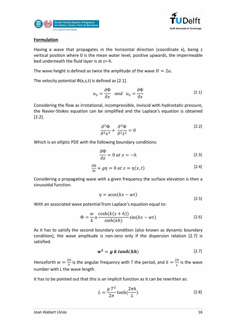
Formulation
Having a wave that propagates in the horizontal direction (coordinate x), being z vertical position where 0 is the mean water level, positive upwards, the impermeable bed underneath the fluid layer is at z=-h.
The wave height is defined as twice the amplitude of the wave � � 2�.
The velocity potential Ф(x,z,t) is defined as [2.1].
�� � �� ���� � ���
Considering the flow as irrotational, incompressible, inviscid with hydrostatic pressure, the Navier-Stokes equation can be simplified and the Laplace’s equation is obtained [2.2]. ��Ф��� � ��Ф���� � 0
Which is an elliptic PDE with the following boundary conditions: ��� � 0��� � ��
��� � �� � 0��� � ��, �� Considering a propagating wave with a given frequency the surface elevation is then a sinusoidal function. � � acos� � !��
With an associated wave potential from Laplace’s equation equal to:
Ф � ! � cosh� �� � ���sinh� �� sin� � !�� As it has to satisfy the second boundary condition (also known as dynamic boundary condition), the wave amplitude is non-zero only if the dispersion relation [2.7] is satisfied. %& � '()*+,�(,� Henceforth ! � �-. is the angular frequency with T the period, and � �-/ is the wave
number with L the wave length.
It has to be pointed out that this is an implicit function as it can be rewritten as:
0 � �1�22 tanh�22�0 �
[2.1]
[2.2]
[2.4]
[2.3]
[2.5]
[2.6]
[2.7]
[2.8]

Joan Alabart Llinàs 17
At this point depending upon the relation between h and L three domains can be distinguished:
- Deep waters: in this case the depth is much bigger than the wave length, thus knowing that the hyperbolic tangent being is an asymptotic function to 1, the relation is written as:
0 � � 1�
22
- Intermediate waters: in this case no simplification can be done and the
equation must be solved via iterative methods such as Newton’s method.
- Shallow waters: in this case when waves are approaching the coast, the depth becomes much smaller than the wave length. Thus using the first term of Taylor’s polynomial for the hyperbolic tangent, the relation is simplified to:
0� � � � 1�
Another interesting feature from the linear wave theory is that underneath the surface the fluid motion is orbital. This can be shown in the following figure.
Figure 2. Orbital motion representation (Wikipedia).
From it, Airy explained that the orbital motion is more reduced the closer a particle is from the bottom. The velocity field and the disturbance pressure field (relative to hydrostatic) die off exponentially with depth. At the same time he explained that being far enough from the sea bed the bottom friction has a negligible effect, therefore this motion is roughly circular whereas the closer to the impervious layer the more elliptical it becomes. From the velocity potential equation [2.1] and [2.6] the horizontal and vertical velocity components can be derived.
Ultimately, other second order wave properties can be described by this theory. The most important of them being:
[2.10]
[2.9]
Joan Alabart Llinàs 18
The mean wave-energy per area 4 � 5�6��� [J/m2]
The radiation stresses: 7�� � 8� � 5�� �9:;�<=4 [N/m]
7>> � 8� � 5�� �;?��<=4
7�> � 7>� � �9:;<;?�<4
The wave action @ � AB � ACDEF [J·s/m2]
The radiation stress is responsible of the set-up and set-down. This is the superelevation of the mean water level caused by wave action. If h is the still water level, and �̅ is the mean water surface elevation the mean water level is governed by the cross-shore balance of momentum: ��̅� � � 16�� �7���
That means that when approaching the coast as Sxx increases, the water level decreases (set-down) until the wave breaks. When that happens as energy dissipates, the water level increases (set-up or run up). For further information about this phenomenon the reader is referred to (U.S.Army_Corps_of_Engineers, 2002) or (Bosboom & Stive, 2013).
2.3. PROPAGATION OF WAVES
The propagation of the waves from the place where they are generated towards the coast is an important phenomenon that maritime and fluid engineers have been trying to understand and model as accurate as possible.
When the waves propagate towards shallow waters, several effects can be identified and in this chapter the most important ones will be briefly described. These are: shoaling and refraction. Furthermore, in harbour domains diffraction around the tips of the breakwaters, reflection against walls and transmission through porous layers play an important role. Ultimately wave breaking along beaches and mould breakwater, and non-linear effects should not be neglected and will be also treated.
Important concepts are the wave celerity, the group celerity and the wave direction.
The wave celerity is the speed at which a single wave propagates.
9 � 01 � �122 tanh�22�0 �
[2.12]
[2.11]
[2.13]
[2.14]
[2.15]
[2.16]
[2.17]

Joan Alabart Llinàs 19
Nevertheless, as explained before monochromatic and unidirectional waves are unlikely to occur in the reality. Therefore, another concept is introduced that is the group celerity. This can be understood as the speed at which the wave energy travels.
9I � �!� � J2 K1 � 2 �;?���2 ��L
2.3.1. SHOALING
Shoaling is the increase in the wave height when waves travel towards shallower waters. The reason for this is that when the water depth decreases, so does the group celerity. Then as the energy flux has to remain constant, the energy density must increase. Besides, while the frequency remains constant (the period too), the wavelength must decrease.
Figure 3. Shoaling scheme Source: The COMET Program.
The shoaling process can be described by means of the shoaling coefficient. This relates the wave height at deep waters and the wave height at the propagated point. It is defined as follows [2.19] and comes from the conservation of the energy flux.
�M � �N ∗ P; � �N ∗ QRISRIT
The group celerity can be obtained deriving w (the angular frequency) from the dispersion relation.
Doing so and rearranging the terms the following compact expression for the shoaling coefficient can be found.
PU � 2V�sinh�2V� � V�1 � cosh�2V����2V � sinh�2V���
[2.19]
[2.18]
[2.20]

Joan Alabart Llinàs 20
Where V is by definition:
�W�� � �X�� � � �E��
5W �W�� � 5X �X�� � 5E �E��
For further details the reader is referred to (Walkley, 1999).
When representing the shoaling coefficient against the depth in a graph, in can be seen that in intermediate waters Ks<1. That means that the wave height is reduced (the minimum is 0.91 at d/λ0≈0.15) (Fenton, 2010). However, when waves approach shallow waters it rapidly increases and tends to infinite for a depth tending to 0. Obviously this never happens in reality because apart from shoaling other processes like wave breaking that limits the wave height occur.
Figure 4. Shoaling coefficient variation with dimensionless depth (Fenton, 2010).
2.3.2. REFRACTION
Refraction is the phenomenon for which wave energy tends to bend when waves approach the shoreline. It is a complex effect but it is due to the bottom friction or currents that reduce the velocity of the waves.
As explained before, when the water depth decreases so does the speed of the waves. Therefore, if a wave is approaching the coast at a certain angle (angle between the wave front and the constant depth lines (e.g. a constant sloping beach)), the points which are closer to the coast will suffer a higher decrease in the group velocity than the ones that are deeper. As a consequence, the wave will bend and the incidence angle will be reduced.
[2.21]
[2.22]
Joan Alabart Llinàs 21
Figure 5. Refraction scheme Source: The COMET Program.
This phenomenon is of major importance because it explains why waves concentrate in headlands and the reason of the spreading of incident energy (and wave height) in bays as the energy per wave length of crest decreases.
Similarly to shoaling, variations in the wave height can be described by means of the refraction coefficient defined as:
PY � Z[:[\
Where Bo is the width between two flux lines (orthogonal to the wave front) in deep waters, and Bp is the width between the same flux lines in the propagated point.
Furthermore, to calculate the variation of the incident the Snell’s law can be applied.
It states that when the celerity of the waves changes, so does the propagation angle. ;?�<];?�<M � J]JM
Knowing that the wave celerity can be calculated with the dispersion relation, the variation in the wave direction can be calculated. Besides, when having a constant sloping bed, the relation Bo/Bp can be related to the relation between the incoming angles in both points as the momentum and mass flux must are conserved.
Nevertheless, the cause of wave refraction is not only the variation of the water depth, but also the presence of currents. Waves propagating along an area where there are important cross currents may refract as well as if they were approaching the coast.
[2.24]
[2.23]
Joan Alabart Llinàs 22
2.3.3. REFLECTION AND TRANSMISSION
When waves hit an obstacle, they bounce off and continue in another direction. Those objects may be quay walls, jetties, natural cliffs, ship hulls, breakwaters or any other structure standing in the sea. In a perfect and ideal environment, if a wave impacts a wall with an incident angle α with the normal to the wall, it is reflected with an angle –α from it.
Figure 6. Combination of wave reflection and refraction scheme (Anthoni, 2000).
Nonetheless, in reality not all the incident energy is reflected; part of it dissipates and part of it is transmitted. The amount of energy reflected, transmitted and dissipated depends on the characteristics of the waves (wave height, period, angle of incidence and breaking state) and proprieties of the obstacle such as the slope, hardness, element size or height (if overtopping happens) (Robert A. Dalrymple et al. 1991). Thus a reflection coefficient is introduced that relates the incoming and reflected wave height.
Ultimately, when the incoming waves are almost perpendicular to the object, the incident and reflected waves interact and generate stationary waves that can have twice the amplitude of the initial waves.
It is important to point out that when it comes to harbour domains as in this study, reflection is one of the most important phenomena that occur. Up to now only the effects of monochromatic unidirectional waves have been described. However, definitely when one account for real wave climates defined by means of a directional and frequency wave spectrum, reflection is neither that easily calculated nor the interaction of the waves that it produces.
Hence, reflection is going to be one of the main elements on which we are going to focus on this study.
Joan Alabart Llinàs 23
TRANSMISSION
When waves hit a porous structure like a breakwater, part of the energy is transmitted through it. The amount of energy transmitted depends on the characteristics of the wave and the porosity, grain size roughness and height of the structure as overtopping may occur (i.e. groins). Long period waves such as tidal or swell waves are more easily transmitted than high frequency waves, which are either dissipated or reflected against the structure. A small study on the reproduction of this effect by SWASH will be carried on in Chapter 4.
In harbour domains it is important to know how much energy is transmitted as it may affect operations inside the port. Moreover, this likelihood of low frequency waves to be transmitted may be the trigger of resonance problems inside the basins that usually end up in catastrophic effects.
2.3.4. DIFFRACTION
When waves propagate through an obstacle, they tend to bend to the “shadow area”. This means that they do not follow a straight line. Furthermore, what happens is that because of the transversal gradient of energy (wave height), there is an horizontal transfer of energy from the points with the higher wave height to those ones in the shadow areas.
Figure 7. Diffraction scheme around a breakwater (R.Boshek, 2009).
Diffracted wave height in the shadow zone can be calculated by means of the modified Sommerfeld’s solution (Penney & Price, 1952). This is given by: ^�Y, <� � _�`�aDbEcdNU�eDef� � _�`g�aDbEcdNU�eDef� With ` � 2QEc- sin�eDef� �`g � 2QEc- sin 8ehef� = _�`� � 5hb� i aDb-�j/�BDl ��
[2.26]
[2.25]

Joan Alabart Llinàs 24
Figure 8. Sketch for Sommerfeld Solution (Daemrich & Kohlhase, 2011)
The two terms of the equation represent the fraction of diffracted and reflected wave energy for totally reflective structures. With only partially reflective obstacles (like breakwaters) the second term must be reduced.
Nevertheless, as one usually encounters irregular sea waves, diffraction must be computed by the introduction of the directional wave spectrum:
�Pm�noo � p 1q]r r 7�_, <�Pm�estuesvw
l] �_, <��<�_x].z
With �Pm�noo � diffractioncoefficientofrandomseawaves P_��_, <� � diffractioncoefficientofregularwaveswithfandθ
Further information in the directional wave spectrum will be provided in section 2.4.
As it happened with reflection, diffraction is another major phenomenon in port domains. The presence of breakwaters, groins, jetties or other structures may produce waves to diffract towards sheltered areas that were wanted to be protected. However, when waves diffract, the energy is spread along a huge area which means that diffracted waves have a smaller height than the incident ones. In preliminary studies or when numerical methods were still not as developed as in present time, approximated solutions can be used to calculate the effect of breakwaters. Those solutions are represented in graphs where knowing the gap or kind of breakwaters, the depth, distance from the tip to the point of interest in the shadow zone, direction of the incident waves and angle between the breakwater and the tip-point line, one can obtain the approximated solution for monochromatic unidirectional waves.
However, for complex geometries and more realistic wave climates numerical phase solving methods must be applied as will be explained in Chapter 3.
[2.27]

Joan Alabart Llinàs 25
2.3.5. WAVE BREAKING
As it has been argued before, waves when propagating towards the coast will increase their height until infinity due to shoaling in absence of a physical limit to the steepness of waves. Nevertheless, when the particle velocity exceeds the velocity of the wave crest, the former becomes instable. This occurs for a crest angle of about 120º. Miche (Miche, 1944) expressed the limiting wave steepness based on Stokes wave theory and obtained the following relation between the wave height and the length of the waves at breaking point.
K�0L��� � 0.142tanh� ��
On the one hand, in deep water this reduces to 1/7. When the steepness exceeds this limit wave breaking occurs (white caping) and a part of the energy is dissipated. This phenomenon is included in models such as SWAN.
On the other hand, in shallow water this criterion can be reduced to the following relation.
� � ���� � 0.88
Where � is the breaker index.
Using solitary wave theory which is a non-linear wave theory valid for shallow waters this value is 0.78 though.
Nonetheless, when it comes to irregular waves, as the wave breaking starts with the maximum wave height and not the significant wave height. The breaker index is then: Hs/h =0.4-0.5.
Ultimately it must be pointed out that those results where only valid for a flat bottom. When it is sloping, the slope plays an important role. The Irribarren parameter is defined as the ratio between the slope of the bottom and the wave steepness and is an indicator of the type of wave breaking. Moreover, when waves brake it seems that they need time, therefore, the steeper the slope the highest de breaker index reaching values up to 1.2. In addition when waves break they generate a layer of air-water mixture which moves in a landward direction in the upper parts over the water column. This is the so-called surface roller and acts as a temporary storage of energy. In Chapter 3 an insight on how does SWASH account for wave breaking will be given.
[2.28]
[2.29]
Joan Alabart Llinàs 26
2.3.6. NON-LINEAR EFFECTS
As explained in the beginning of this chapter, linear wave theory is only valid when the wave amplitude is much smaller than the water depth. In such a situation the advective (non-linear) term can be neglected and the sinusoidal wave solution achieved. Furthermore in linear wave theory the boundary conditions are applied to the mean water surface z=0 instead of the instantaneous water surface �.
However, when approaching the coast, this assumption becomes less and less realistic and non-linear effects start playing a role. These non-linear effects can be wrap up in two phenomena. Wave skewness and wave asymmetry.
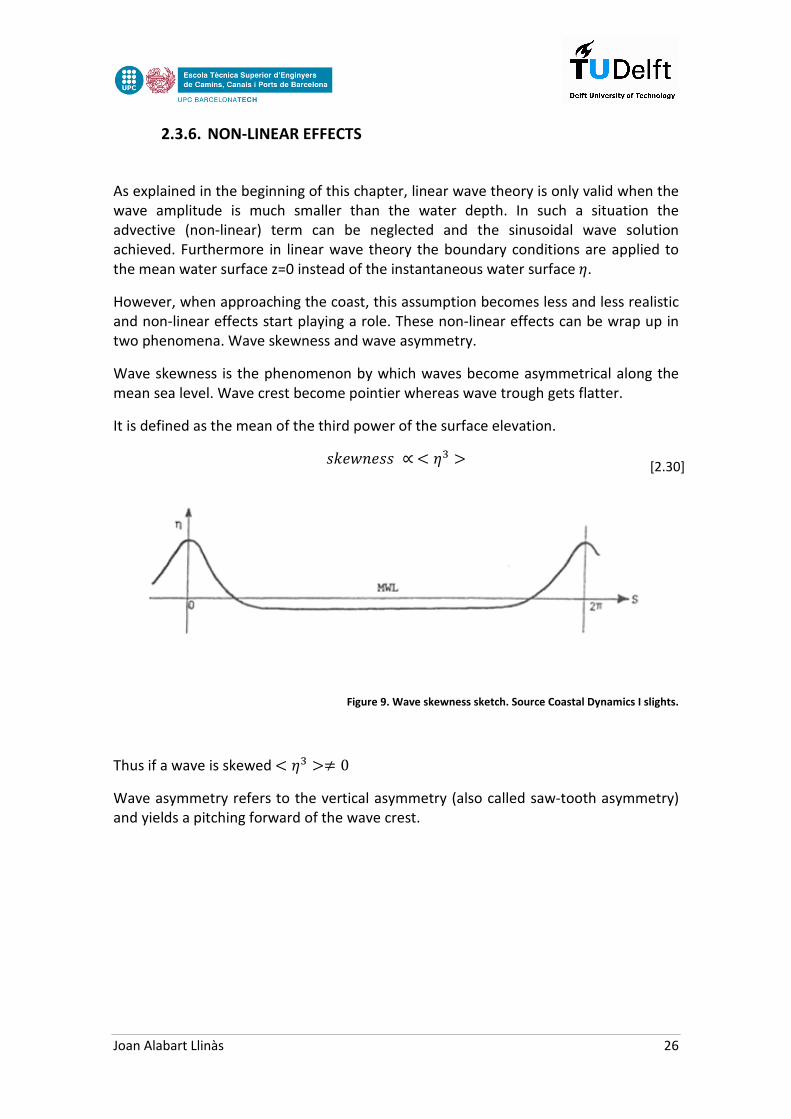
Wave skewness is the phenomenon by which waves become asymmetrical along the mean sea level. Wave crest become pointier whereas wave trough gets flatter.
It is defined as the mean of the third power of the surface elevation. ; a!�a;; ∝� �� �
Figure 9. Wave skewness sketch. Source Coastal Dynamics I slights.
Thus if a wave is skewed � �� �� 0
Wave asymmetry refers to the vertical asymmetry (also called saw-tooth asymmetry) and yields a pitching forward of the wave crest.
[2.30]

Joan Alabart Llinàs 27
Figure 10. Wave asymmetry sketch as a sum of two harmonics dephased. Source Coastal Dynamics I slights.
The reason for this asymmetry is that the crest in shallow water moves faster than the trough.
For non-linear wave theories, the free surface boundary conditions have to be applied at the free surface �. The issue is that � is unknown. There are several non-linear theories that have been developed so far (Bosboom & Stive, 2013).
Stokes series expansion. This methodology uses the results from the linear wave theory by adding more harmonic terms to the solution. Each new term has a lower period and these terms can be out of phase. Therefore the solution looks like: � � �59:;7 � ��9:;27 � ��9:;37…
By dephasing the different harmonics wave asymmetry is achieved as was shown in figure 10. However, this theory does not converge in shallow water if the Ursell number is too large.
Stream function theory: Is similar to the Stokes theory also adding higher harmonics to the linear solution.
Cnoidal wave theory: This theory is applicable in shallow water and solutions are given in terms of elliptic integrals of the first kind. In deep water it is equal to the linear wave theory whereas in shallow water it resembles the Solitary wave theory that is a single wave without a trough.
Boussinesq models: Are an expansion of the shallow water equations. They describe non-linear waves, with non-hydrostatic pressure and include frequency dispersion. Since the equations can still be integrated over the vertical they are computationally efficient.
[2.31]
Joan Alabart Llinàs 28
2.4. WAVE ANALYSIS
Until now waves have been treated as if they were always monochromatic and unidirectional. However, in reality those waves seldom exists, and a statistical analysis is required to be able to know the wave climate and work with the most relevant parameters.
Usually buoys register by means of a pressure sensor or other devices the water surface elevation. To know the wave heights a zero crossing analysis must be done. With an event with N waves, a wave height that represents this wave climate is required. This is done by using the maximum wave height Hmax or the significant wave height H1/3. The second one is obtained by ordering the waves and doing the mean of the highest 1/3.
The same can be done by using the p first waves (highest) and obtaining then Hp. It is important to note that H1 is the mean wave.
Another important value is the root-mean-square wave height for a group of waves HRMS. This can be calculated as follows:
���� � �1���b��b�5
Also important is the variance σ2 of the waves which is related to the wave energy. It can be shown that assuming small amplitudes compared to the wave length, the kinetic and potential energy are the same and thus the total energy per unit area of the waves can be defined as: 4 � 6�`�
2.4.1. RAYLEIGH DISTRIBUTION
As a simplification, it can be assumed that the sea surface is composed of a sum of a large number of sinusoids. If those functions have a similar frequency (narrow-banded sea) it can be demonstrated that the cumulative probability function of the wave height follows a Rayleigh distribution (Dean & Dalrymple, 1984). That means that:
��� � � ¡ � �� � aDK ¢ ¢£¤¥Lj
[2.32]
[2.33]
[2.34]
Joan Alabart Llinàs 29
Being n=pN it can be rewritten as:
� � ����Z¦� 1\
From what the mean wave height is: �§ � 0.886 ∗ ����
2.4.2. SPECTRAL ANALYSIS
Another important way of analysing the wave climate is by means of the wave spectrum. That means analysing the frequency domain instead of the time records. This is achieved using the Fourier transforms.
���� � ��© cos�22_©� � ª©��©�5
The sea surface (a continuous function) can be written as a sum of sinusoidal functions with different frequencies, phases and amplitudes. The terms �© indicate how much each sinusoidal function contributes (is the projection) whereas ª© determines de phases. Those coefficients can be calculated by solving certain integrals (Dean & Dalrymple, 1984) and it can be done by computer using the FFT (Fast Fourier Transform) algorithm which yields both parameters. This is an extremely efficient algorithm to calculate the Fourier coefficients for an input time series record. It is important to point out, that the minimum frequency is related to the length of the time series which should be around 15-20 mins and the maximum frequency that is related to the sampling frequency.
_�b© � 5.« _��� � 5�∆� With it, it can be plotted in a graph the amplitude spectrum (�©;_©�. However, it is
even more interesting to plot �wj�∆o that gives the variance density spectrum. The graph
variance density vs frequency is extremely important and it can be proved that the area below this graph is equal to the variance of the signal and, therefore, related to the wave energy with a factor6�.
Moreover, the statistic moments can be defined as:
mn�r fn∞0 E�f�df
Being f the frequency, and E(f) the variance density spectrum.
[2.37]
[2.36]
[2.35]
[2.39]
[2.38]

Joan Alabart Llinàs 30
Defining the bandwidth parameter as [2.40] that gives information on how narrow is the spectrum.
° � Z±1 � q��q]q²³
The main wave parameters can be found.
Assuming that the wave heights follow a Rayleigh distribution, it can be proved that the significant wave height is:
�5 �⁄ � ��] � 4Zq] ±1 � °�2 ³ ≅ 4¶q]
In reality this relation has a factor of 3.8 instead of 4 (Bosboom & Stive, 2013).
Furthermore, a relation between HRMS and Hs can be drawn: �; � √2 ∗ ����
The average wave period then is related to the 2 first spectral moments as:
1̧ � q]q5
The mean zero crossing period is related to the 0 and 2nd spectral moments. This period overweighs the high frequency components with lower energy density as it includes a high order moment.
1̧ � Zq]q�
Tav: This period overweights the values of the low frequency components where the energy density is higher. It is better to use this mean period than the previous one.
1�¹ � ZqD5q5
[2.41]
[2.40]
[2.42]
[2.43]
[2.44]
[2.45]
Joan Alabart Llinàs 31
2.4.3. DIRECTIONAL SPECTRUM
Nevertheless, in reality the waves are not coming always from the same direction. To account for this the concept of directional spectrum is introduced. This new spectrum is defined as follows: 4�_, <� � 4�_� ∗ ºo�<�
This means that for each frequency a function ºo�<� distributes this frequency along
the different wave directions. This function is defined as:
º�<� � 12 »12 ��¼�© cos��<� � ½© sin��<�¾l©�5 ¿
However according to buoy measurements only the lowest 4 initial Fourier terms are known (a1, b1, a2, b1). Furthermore, this spectrum is not always positive, it can achieve negative values. For this reason it is more commonly used the cosine power distribution. This cosine power can be either simple with two parameters:
º�<� � @9:;�U�eDÀf� � Where s is the one-sided directional spread and ª] is the mean wave direction. Or it can be more complex including 4 parameters:
º�<� � @59:;�U5 8e�= � @�9:;�U��eDÀf� � Both those two spectra have skewness equal to 0.
A relation between the four Fourier coefficients and the most significant parameters referring to the distribution was done by (Kuik, Vledder, & Holthuijsen, 1988). To summarize the main points of that paper, they defined the linear moments of º�<� and related them to the standar deviation, the skewness and the kurtosis. In addition, they defined the circular moments and related them to the 4 Fourier parameters (a1, b1, a2, b1). They performed a series of analysis to check which combinations of parameters fitted better the measurements. For further information the reader is addressed to (Kuik et al., 1988) that gives a comprehensive explanation of the topic.
[2.46]
[2.47]
[2.48]
[2.49]
Joan Alabart Llinàs 32
2.4.4. IDEALIZED SPECTRA
It is often useful to define idealized wave spectra which broadly represent the characteristics of real wave energy spectra.
Some commonly used spectra are the Bretschneider or ITTC which is a two parameter spectrum, the JONSWAP (JOint North Sea WAve Project) for coastal waters where the fetch is limited based in the ITTC, the DNV spectrum and the Pierson Moskowitz.
In SWASH some of them can be used to input the wave conditions and in this thesis the JONSWAP directional spectrum will be used as the fetch in the Mediterranean Sea is quite limited. In this spectrum the required inputs are the peak period, the significant wave height, the mean wave direction, the wave directional spreading and the period at which the spectrum is repeated.

Joan Alabart Llinàs 33
[3.1]
[3.2]
CHAPTER 3: WAVE PROPAGATION MODELLING
3.1. BACKGROUND
In this chapter an overview of the different models that exist to simulate the propagation and generation of waves will be provided. The starting point is the Navier-Stokes equation that can explain most of the problems that relate to fluid mechanics. This equation arises from the application of Newton’s second law: conservation of momentum, and from the assumption that the fluid stress is the sum of a diffusing viscous term and a pressure term.
6 KºÁº�L � 6 K�Á�� � Á ∙ ÃÁL � �Ã\ � à ∙ Ä � Å
On the left hand side the total derivative relates to the acceleration that is equal to the local derivative plus the convective derivate. On the right hand side there are the pressure term, the deviatoric stress tensor and the external body forces (per unit of volume).
This equation is the most general equation relevant to all fluid mechanics problems. However, as until now no exact solution has been found for it, some hypotheses have to be made in order to simplify the problem.
On the basis of certain assumptions related to the stress tensor, equation [3.1] can be rewritten in the following form for compressible, stokesian fluids:
6 K�Á�� � Á ∙ ÃÁL � �Ã\ � μÃ�Á � �1
3 Ç � ǹ�Ã�à ∙ Á� � Å
µ is de dynamic viscosity and µv is the volumetric viscosity.
If the fluid is incompressible (or if the compressibility is too small to have a significant effect) µv=0 and à ∙ Á= 0 from the continuity (mass) equation.
Making several assumptions concerning stationary flow, incompressible, irrotational, hydrostatic pressure, the Laplace equation that describes the linear theory explained in Chapter 2 is found.
Nonetheless, the hypothesis that the pressure is hydrostatic may be realistic in deep waters, but when waves approach shallow waters and the effects of wave skewness, wave breaking, run up and currents appear, a non-hydrostatic term has to be taken into account.
Moreover, to describe the propagation of waves through water, the shallow water equations are used. They are the simplest form of the equations of motion that can be used to describe the horizontal structure of an atmosphere and the response of an
Joan Alabart Llinàs 34
incompressible fluid when it is subjected to gravitational and rotational accelerations (Randall, 2006).
However, those equations do not have yet an exact solution, and numerical methods are used to approximate them. At the same time, as many assumptions are made to simplify the governing equations, each numerical model uses a certain type of equations that are only applicable in certain cases. This is the reason why there are several different models as each one has its own scope of applicability.
3.2. MODELS AVAILABLE
This section will discuss the main features of the most common models available at present. First of all, there are spectral wind-wave equation models for wave propagation in open water where the main processes are wind input, shoaling and refraction. Moreover parabolic mild-slope equation models try to simulate wave propagation over large coastal areas with negligible reflection. Besides, when it comes to harbour domains there are models that focus on wave agitation and harbour resonance using the Helmholtz equation, elliptical mild-slope models in water of varying depth, and Boussinesq models for nonlinear wave refraction-diffraction in shallow water (Nwogu & Demirbilek, 2001).
Examples of models are STWAVE as a spectral wind wave model, CGWAVE as a mild-slope model or BOUSS-2D as a Boussinesq model. All of them have been developed by the U.S. Army Corps of Engineers.
Another important model that is widely used is PHAROS that calculates the solution of the elliptic mild-slope equation formulated by Berkhoff (1972). This equation governs linear wave propagation over a mildly sloping bathymetry, with no restrictions upon the water depth (Deltares systems).
However, TU Delft has been developing its own models; each one with its own range of applicability.
On the one hand it can be found WAVEWATCH III (Tolman 1997, 1999a, 2009) as a third generation model that solves the random phase spectral action density balance equation and whose applications are mainly for ocean waves (deep waters).
Furthermore another widespread model that has been developed by this university is SWAN (Simulating WAves Nearshore) that is based on the wave action balance equation with sources and sinks. It is a phase average model whose applications are mainly in shallow waters with slowly varying wave environments.
Ultimately, one can find SWASH (Simulating WAves till SHore), that has also been developed by TU Delft, as a phase solving model that uses as its governing equations the nonlinear shallow water equations including non-hydrostatic pressure (Zijlema &

Joan Alabart Llinàs 35
Stelling, 2008). Its applicability as explained in this document is for shallow water domains with rapidly varying environments.
3.3. PHASE AVERAGED AND PHASE SOLVING MODELS
An important categorization of wave models is the one done by Battjes (Battjes, 1994) when referring to the approach followed to represent the wave field. A distinction can be made between phase average models (e.g. SWAN) and phase solving models (e.g. SWASH).
Phase average models operate in the frequency domain and are based on the energy or action balance equations by adding the required physical processes using other numerical techniques (Booij, Ris, & Holthuijsen, 1999). They can be of a Lagrangian nature or Eulerian nature as SWAN.
On the one hand, the Lagrangian models propagate the waves from deep water to the shore by transporting the wave energy along a wave (Cavaleri & Malanotte-Rizzioli, 1981; Collins, 1972). However, they are numerically inefficient when non-linear effects appear. On the other hand, Eulerian models formulate the wave evolution on a grid. They do not determine the exact location of the sea surface elevation and the results correspond with a picture of the wave field averaged characteristics (Guzmán, 2011).
Phase solving models on contrary operate in the time domain. Hence, they calculate the position of the sea surface elevation field for each time step during the period required. In those models the results (outputs) are a set of pictures of the surface elevation fields for each time step. However, they require post processing to obtain important parameters as wave heights and periods (Guzmán, 2011). There are four types of phase solving models related to the equation they solve: Boundary Integral, Boussinesq, Mild Slope Equation and Non-Linear Shallow Water equation (NLSW henceforth) like SWASH.
In domains where local wave properties vary strongly in distances smaller or similar to the wave length, it is better to use phase solving models. Phase average models are more adequate in slowly varying environments with weak variations of the wave properties within a wavelength scale, allowing the wave field to be considered quasi-uniform.
An important issue of phase average models is that they are not able to reproduce reliably simulations neither of diffraction nor reflection nor other non-linear effects. On the other hand, phase solving models do not include wind effects on wave transformation.
Nonetheless, the main drawback of phase solving models is that they are much more expensive computationally than phase average as they describe the sea surface in time and space. This is the reason why they are applied in small domains or where they are

Joan Alabart Llinàs 36
strictly needed as in harbour basins or around breakwaters, groins or other coastal structures.
Model SWAN SWASH
Developer TU DELFT TU DELFT
Version 40.91 1.20
Type Phase average Phase solving
Equations Action balance Non-linear shallow water equations
Applicability Slowly varying environments Rapidly varying environments
Advantages Fast – Broadly tested Accurate
Drawbacks Bad diffraction and reflection
Works in the spectral domain
Time consuming
Small domains
Early stage
Table 2. Comparison between SWAN and SWASH.
3.4. SWASH
SWASH is a general-purpose numerical tool for simulating non-hydrostatic, free surface, rotational flows. It provides a general basis for describing complex changes in rapidly varied flows and wave transformations in coastal waters. This recently released model is developed in the TU Delft and has an open source available in the “sourceforge” webpage and is still in developing process. The current version is 1.20.
SWASH is a phase resolving model, which makes it suitable for rapidly changing conditions within the scale of the wave length.
GOVERNING EQUATIONS
As explained before, SWASH is based on the Non-Linear Shallow Water equations including a non-hydrostatic pressure term. These hyperbolic equations can be obtained from the Navier-Stokes equation for an incompressible and inviscid fluid with constant density 6] and are the following:

Joan Alabart Llinàs 37
[3.4]
[3.3]
[3.5]
��� � �C� � 0
���� � ���� � �!��� � �6] ��� � 16] �� � 0 �!�� � ��!� � �!��� � 16] �� � 0
Where ��, �, ��and !�, �, �� are the mean velocity components in the horizontal X and vertical Z directions; g is the gravity acceleration and �, �, �� is the non-hydrostatic pressure. It is important to point out that the pressure is separated between the hydrostatic component ��� � �� and non-hydrostatic component q. Finally � is the free surface position.
This system of equations has four boundary conditions (Zijlema & Stelling, 2008).
- Free surface with pressure É| �Ë � 0 as no wind is assumed.
- Bottom without bottom friction and with normal velocity imposed through the
kinematic condition !| �Dm � �� �m��.
- At the offshore boundary usually the water level is specified and q=0 is assumed, as a consequence the wave enters as a shallow water wave. To avoid mismatches in the deep water wave amplitude it is imposed the depth-averaged velocityÌ � �!� �⁄ .
- The moving shoreline is the last boundary condition and it has a numerical treatment with an algorithm that defines wet and dry points being the threshold 0.1m below the bottom.
Finally in order to calculate the water surface elevation the continuity equation is integrated over the water depth. Using the kinematic condition at the free surface !| �Ë � ��/�� � ���/� gives the following free-surface equation: ���� � �Í�� � 0,Í � Ì� � r ���Ë
Dm
For further details it is recommended to review Zijlema and Steeling (2008 and 2003).
With those equations, all the physics are contained in the equations and thus no approximations should be done nor added as source or sink terms as it usually happened with phase-average models.
Nevertheless, the drawback of those equations is that it is not possible to input energy as wind, as it is done in wave generation models like WAVEWATCH III or SWAN.
Momentum
conservation
equations
Mass conservation
equation
Joan Alabart Llinàs 38
[3.6]
MAIN FEATURES
SWASH is based on an explicit, second order finite difference method for staggered grids reason for what mass and momentum are strictly conserved at discrete level.
When it comes to the time integration, as it uses an explicit method (it can be run in implicit mode for 1D though) it may have stability problems. To avoid them, the Courant-Friedrichs-Lewi condition (more known as Courant number) has to be satisfied.
This condition is given by the following inequation in 2D domains (Nwogu & Demirbilek, 2001).
J� � ZÎJ�∆�� K 1∆� � 1∆Ï�LÐ � 1
Where C is the phase speed, and ∆�, ∆, ∆Ï the time and spatial discretizations.
However it is recommended to keep the Courant number within the range 0.5 to 0.7 in order to prevent instabilities coming from non-linear phenomena.
Furthermore, SWASH accounts for this by introducing a time step control that doubles or halves the ∆� for each time step depending upon this number.
Another important feature of this model is that it can be run either in depth-averaged mode or multi-layered mode. In the latter mode the computational grid is divided into a fixed number of vertical terrain-following layers. Thus, instead of increasing the frequency dispersion by increasing the order of derivatives of the dependent variables like Boussinesq-type models (e.g. BOUSS 2D), SWASH accounts for it by increasing the number of vertical layers. Moreover it contains at most second order spatial derivatives.
SWASH allows for the following physical phenomena.
- Propagation, frequency dispersion, shoaling, refraction and diffraction. - Nonlinear wave-wave interaction. - Wave run-up and run-down and wave breaking - Moving shoreline. - Bottom friction. - Partial reflection and transmission. - Wave-induced currents and wave-current interaction. - Vertical turbulent mixing. - Subgrid turbulence. - Mass and momentum conservation. - Rapidly varied flows.

Joan Alabart Llinàs 39
All those phenomena can be simulated with different schemes. For instance to account for bottom friction, the user can chose between the formulations of Manning, Chezy or Nikuradse.
SWASH LIMITATIONS
However, the current version of SWASH (1.20) does account neither for wind effects on wave transformation nor for hotstarting as SWAN does. Furthermore, as SWASH is based in a finite difference scheme, by now it is not possible to use unstructured meshes and only regular or curvilinear ones are permitted.

Joan Alabart Llinàs 40
[4.1]
[4.2]
CHAPTER 4: POROUS STRUCTURES
4.1. INTRODUCTION
In harbour domains one of the most important features that can be found are porous structures such as groins, mould breakwaters, submerged structures or even quay walls. All those structures have an effect in the wave propagation. They can reflect the energy, transmit it or dissipate it even though most of the times the result is a combination of these three effects. Previous models such as SWAN accounted for those structures simply inputting a reflection and transmission coefficients that could be frequency dependant. The reason for it is that as they worked in the frequency domain by solving the wave action equations it was straightforward to transmit energy or reflect it in that way. It must be pointed out that this approach has some important lacks as in reality the frequency is not the only factor that determines how much energy is transmitted/reflected. Other parameters such as wave height, porosity, size of the porous elements or even wave direction play important roles when determining these coefficients.
However, SWASH as it works with the water surface elevation and the flow velocities has a totally different approach to account for the porous structures as will be explained in the following sections.
4.2. BACKGROUND ON POROUS STRUCTURES
This section will provide an overview of the actual state of the art when it comes to porous structure treatment.
First of all, the filter velocity will be defined. It is the actual pore velocity averaged over the pores. This is the ratio between the volumes of pores over the total volume multiplied by the flow velocity.
�o � �� � ÑÒÑÓ �
Using this filter velocity, Forchheimer modified the Darcy equation by adding a quadratic term (Mellink, 2012). Ô � ��o � ½�o|�o| In this equation I is the hydraulic gradient and a and b are the laminar and turbulent coefficients.

Joan Alabart Llinàs 41
[4.3]
[4.4]
[4.5]
[4.6]
[4.7]
[4.8]
The linear term is associated to the laminar flow while the non-linear term corresponds to the turbulent part of the flow.
By derivating the Forchheimer formula from the Navier Stokes Equation the following relation can be found:
Ô � ª �1 � ����� Õ��©z]� �o � Ö �1 � ���� 1��©z] �o�
The constants ª and Ö have to be experimentally determined and are only applicable for a certain flow regime.
If the flow is non-stationary an additional coefficient should be added to account for the effect of inertia (Polubarinova-Kocina, 1962). This yields to the next relation:
Ô � ��o � ½�o� � 9 ��o��
Nevertheless, (Van Gent, 1992) concluded that the parameters of the stationary formula are not equal for the non-stationary equation. He split the Ö term in a stationary and non-stationary term Ö�� which he related to the KC number.
Ö�� � Ö K1 � 7.5PJL
With
PJ � Ì 1M��©z]
The Keulegan-Carpenter (KC) number determines how stationary is the flow and represents the magnitude of the convective acceleration term over the local acceleration term (Mellink, 2012).
When it comes to the inertia term, very little is known and there are several formulations for it.
On the one hand, (Burcharth & Andersen, 1995) derived the following equation:
9 � 1 � J� 5D©©�
With J� � 1.5 � 12�1 � �� It is important to mention that this relationship was obtained from a limited amount of experiments.
An alternative formulation was derived by (Van Gent, 1992).
Joan Alabart Llinàs 42
[4.10]
[4.9]
[4.11]
[4.12]
9 � 1 � � 5D©©��
However, as (Mellink, 2012) explains, the inertia term when compared to the laminar and the turbulent terms is almost negligible. Thus it is usually not taken into account.
For further details in the different theoretical formulations for porous flow the reader is referred to (Mellink, 2012) who gives a detailed overview on all the formulations.
4.3. POROSITY IN SWASH
The porosity is accounted in SWASH by including the Forchheimer relation in the porous momentum equation by means of two extra terms fl and ft. With it every grid cell has a porosity that goes from n=0 (impervious layer e.g a wall) until n=1 (pure water).
The governing momentum equation is then
1� ���� � 1�� ���� �⋯� _Ú� � _��|�| � 0 Being:
_Ú � ªA �1 � ����� Õ�� , _� � Ö 1 � ��� 1� It is important to point out that the laminar coefficient is not exactly the one explained before. The following correction must be made: ª � ªA��1 � ��
The default values in SWASH for those coefficients are α] = 1000 and β] � 2.8.
However, as (Mellink, 2012) concludes, these coefficients should be calibrated if enough information is known provided that according to his study SWASH tends to underestimate reflection while overestimates transmission. Nonetheless, in this thesis as the amount of information is limited and not accurate enough, these coefficients will not be modified.

Joan Alabart Llinàs 43
In conclusion the mechanism that SWASH uses to account for the porosity is the inclusion of two additional dissipative terms in the momentum equation. These terms are dependent upon the following characteristics:
- Porosity (inputted in SWASH). - Grain size (inputted in SWASH). - Flow velocity (this depends on many other wave factors such as the period,
wave length, amplitude or water depth).
Furthermore, nowadays in SWASH the porous layers can only be defined in the X and Y directions, this means without variation in depth for a same location. Besides, only a single value of the ª and Ö coefficients for all the grid points can be inputted. Moreover, these added dissipation terms are only present in the horizontal momentum equation and should be added in the vertical momentum equation as well.
4.4. SIMPLIFIED 1D CASES ANALYSIS
In order to have a feeling and check how does SWASH account for porous structures, several simple cases have been simulated to try to relate the reflection and transmission coefficients when changing parameters either from the structure itself (porosity and grain size) or from the incoming waves.
The layout of the initial cases is a 300x300m domain, with a porous structure of 2m width located at 200m from the boundary condition that propagates the waves. The depth is constant and equal to 10m. The waves are unidirectional and monochromatic with a period of 10s, a wave height of 0.05m and a propagation direction perpendicular to the boundary and to the breakwater. With it the wave length is roughly 92m. The porosity is 1 in the entire domain except in the breakwater where it depends on the case. The grain size has been taken as 0.025m. In these cases both friction and viscosity are neglected. The grid size is 2m and the initial time step 2ms. The computational time is 3 minutes and the output is a HRMS map of the domain during the last 100s of computation. To calculate the reflected wave height the incoming wave height has been subtracted from the maximum standing wave height in the reflection zone. This method is quite simple and reasonably accurate though is a rough estimation. The transmitted wave height has been calculated doing the mean of the wave height in the transmitted zone. It is important to realize that some reflection may occur against the northern boundary producing a small error in this coefficient. Still this reflection is small and for the purpose of this analysis is not taken into account though a small overestimation of the transmission coefficient may be expected.

Joan Alabart Llinàs 44
HRMS MAP
199 199.5 200 200.5 201 201.5 202 202.5 203
0
50
100
150
200
250
300 0
0.01
0.02
0.03
0.04
0.05
0.06
0.07
0.08
0.09
0.1HRMS MAP
199 199.5 200 200.5 201 201.5 202 202.5 203
0
50
100
150
200
250
300 0
0.01
0.02
0.03
0.04
0.05
0.06
0.07
0.08
0.09
0.1
The results for porosity n=0, n=0.1, n=0.5 and n=0.7 are shown in the next figure. The results from the other simulations can be found in Annex 3.
From the previous results it can be seen that, as expected, the transmission increases when increasing the porosity. The tendency in this particular case is shown in the next graph where the porosity has taken values of 0 - 0.1 - 0.3 - 0.5 - 0.7 - 0.9 - 1.
HRMS MAP
199 199.5 200 200.5 201 201.5 202 202.5 203
0
50
100
150
200
250
300 0
0.01
0.02
0.03
0.04
0.05
0.06
0.07
0.08
0.09
0.1HRMS MAP
199 199.5 200 200.5 201 201.5 202 202.5 203
0
50
100
150
200
250
300 0
0.01
0.02
0.03
0.04
0.05
0.06
0.07
0.08
0.09
0.1
Figure 11. HRMS map for n=0 (left) and n=0.1 (right).
Figure 12. HRMS map for n=0.5 (left) and n=0.7 (right).
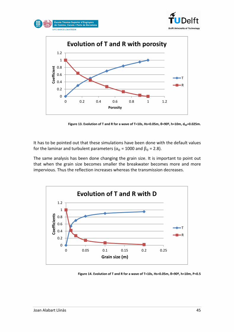
Joan Alabart Llinàs 45
Figure 13. Evolution of T and R for a wave of T=10s, Hs=0.05m, θ=90º, h=10m, d50=0.025m.
It has to be pointed out that these simulations have been done with the default values for the laminar and turbulent parameters (α] = 1000 and β] = 2.8).
The same analysis has been done changing the grain size. It is important to point out that when the grain size becomes smaller the breakwater becomes more and more impervious. Thus the reflection increases whereas the transmission decreases.
Figure 14. Evolution of T and R for a wave of T=10s, Hs=0.05m, θ=90º, h=10m, P=0.5
0
0.2
0.4
0.6
0.8
1
1.2
0 0.2 0.4 0.6 0.8 1 1.2
Co
eff
icie
nt
Porosity
Evolution of T and R with porosity
T
R
0
0.2
0.4
0.6
0.8
1
1.2
0 0.05 0.1 0.15 0.2 0.25
Co
effi
cien
ts
Grain size (m)
Evolution of T and R with D
T
R
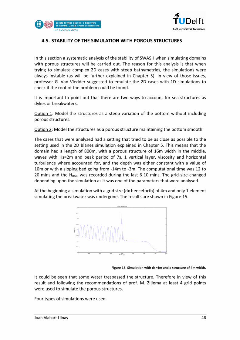
Joan Alabart Llinàs 46
4.5. STABILITY OF THE SIMULATION WITH POROUS STRUCTURES
In this section a systematic analysis of the stability of SWASH when simulating domains with porous structures will be carried out. The reason for this analysis is that when trying to simulate complex 2D cases with steep bathymetries, the simulations were always instable (as will be further explained in Chapter 5). In view of those issues, professor G. Van Vledder suggested to emulate the 2D cases with 1D simulations to check if the root of the problem could be found.
It is important to point out that there are two ways to account for sea structures as dykes or breakwaters.
Option 1: Model the structures as a steep variation of the bottom without including porous structures.
Option 2: Model the structures as a porous structure maintaining the bottom smooth.
The cases that were analyzed had a setting that tried to be as close as possible to the setting used in the 2D Blanes simulation explained in Chapter 5. This means that the domain had a length of 800m, with a porous structure of 16m width in the middle, waves with Hs=2m and peak period of 7s, 1 vertical layer, viscosity and horizontal turbulence where accounted for, and the depth was either constant with a value of 10m or with a sloping bed going from -14m to -3m. The computational time was 12 to 20 mins and the HRMS was recorded during the last 6-10 mins. The grid size changed depending upon the simulation as it was one of the parameters that were analysed.
At the beginning a simulation with a grid size (dx henceforth) of 4m and only 1 element simulating the breakwater was undergone. The results are shown in Figure 15.
Figure 15. Simulation with dx=4m and a structure of 4m width.
It could be seen that some water trespassed the structure. Therefore in view of this result and following the recommendations of prof. M. Zijlema at least 4 grid points were used to simulate the porous structures.
Four types of simulations were used.
0 100 200 300 400 500 600 700 8000
0.5
1
1.5
2
2.5
3
3.5
4
Position (m)
HR
MS
(m
)
HRMS last 10 mins

Joan Alabart Llinàs 47
Simulation A: Structure in the bottom file; depth constant.
Simulation B: Structure as a porous layer; depth constant.
Simulation C: Structure as a porous layer; sloping bed.
Simulation D: Structure in the bottom file; sloping bed.
At the beginning the height of the structures (in simulations A and D) was set to +5m above MSL because the maximum standing wave that could be expected would have had a height of 4m and thus no overtopping should happen.
However, in simulation A the results for dx=4m and dx=2m were the following:
Figure 16. Simulation A with dx=4 (above) and dx=2m (below).
It could be seen that the simulations were not realistic at all and for dx=2m overtopping occurred. Moreover, the simulations with dx=1m and dx=0.5m were instable.
A simulation with a sloping bed structure was carried out. The slopes of the breakwater were set to 1H 2V. The results were the following:
0 100 200 300 400 500 600 700 800-10
-8
-6
-4
-2
0
2
4
6
Position (m)
HR
MS
(m
)
HRMS last 10 mins
0 100 200 300 400 500 600 700 800-10
-8
-6
-4
-2
0
2
4
6
8
10
Position (m)
HR
MS
(m
)
HRMS last 10 mins

Joan Alabart Llinàs 48
Figure 17. Simulation A with sloping side structure. Dx=4m. Monochromatic waves.
The results were the same for the 4 sizes of the grid. Therefore the conclusion was that the steeper the bed, the more instable the simulation became.
Further simulations were carried on with the settings from A but with irregular waves, the results were quite the same. The thinner the grid, the more instable it becomes. Annex 3 contains all the figures and Annex 1 the input files.
The next step was to use porous structures instead of a variation on the bed to simulate the structures. Simulations B and C did this and showed the following results for regular and irregular waves far all the grid sizes:
Figure 18. Simulation B. Regular waves (above) and irregular waves (below).
0 100 200 300 400 500 600 700 800-10
-5
0
5
Position (m)
HR
MS
(m
)
HRMS last 10 mins
0 100 200 300 400 500 600 700 8000
0.5
1
1.5
2
2.5
Position (m)
HR
MS
(m
)
HRMS during the last 10 mins
0 100 200 300 400 500 600 700 8000
0.5
1
1.5
2
2.5
3
3.5
4
Position (m)
HR
MS
(m
)
HRMS during the last 10 mins

Joan Alabart Llinàs 49
Therefore, with porous structures the simulation was always stable and it yielded realistic results.
The results from simulation D can be found in Annex 3.
The results are summarized in the following table:
Case Structure BED PROFILE Dx=4m Dx=2m Dx=1m Dx=0.5m
A1 BOTTOM FLAT
B1 POROUS LAYER FLAT
C1 POROUS LAYER SLOPING
D1 BOTTOM SLOPING
Table 3. Summary of the 1D cases without changing the discretization settings.
Green: STABLE
Yellow: STABLE MONOCHROMATIC WAVES BUT INSTABLE WITH IRREGULAR WAVES
Red: INSTABLE
However, the problems with the steep bottom features and the instabilities with 2D simulations when using porous structures were not solved yet. After a series of trial and error simulations changing the numerical settings for the discretization of the equations, the amount of vertical layers, the inclusion of vertical porosity and other parameters, it was found that if the discretization was set to a first order upwind scheme for the u/v momentum equation, the w-momentum equation and the discretization of the water depth in velocity points, the simulation not only turned out to be stable, but also provided extremely realistic results.
This setting is:
DISCRET UPW UMOM H FIR
DISCRET UPW WMOM H FIR
DISCRET CORRDEP FIR

Joan Alabart Llinàs 50
The results from simulation A with this setting and an increase of the height of the structures to +99m to avoid overtopping were for all the grid sizes then:
Figure 19. Modified A simulation with new setting and height structures of 99m.
Therefore it seemed that with this modification in the discretization schemes the 1D simulations were stable and realistic no matter how you modelled the structures. Thus this setting seems to be the cornerstone for the stability of the 2D simulations as will be explained in Chapter 5.
0 100 200 300 400 500 600 700 800-10
-8
-6
-4
-2
0
2
4
Distance (m)
HR
MS
(m
)
HRMS during the last 10 mins

Joan Alabart Llinàs 51
CHAPTER 5: REAL CASE OF THE PORT OF BLANES
5.1. INTRODUCTION
The Port of Blanes is going to be the real case analysed in this thesis and used to check the performance of SWASH in a real environment. This port has been chosen because this thesis is the result of a project carried on between the UPC and TU Delft. Thus it was agreed that the former would provide the wave climate and port information whereas the latter would provide the software. In addition the author of this thesis is quite familiar with Blanes and its port.
This small harbour is located in the Catalan Coast 70km north from Barcelona. Its principal activities are fishery and nautical leisure and it underwent an expansion that finished in June 2012. It can be seen that the new layout consist basically of 3 basins where small fishing boats and medium sized yachts are moored. Inside the harbour there is a beach that acts as a damping region and landing for the smaller boats. The entrance is oriented towards the west with no appreciable approach channel as the dimensions of the ships are reduced. The protection structures are an outer dyke and a breakwater with some mound protection towards the entrance, and a small counter dike located in shallower waters. The overall dimensions of the port are roughly 500x500m2.
Figure 20. Plan view of the Port of Blanes during year 2013. Source Google Earth.
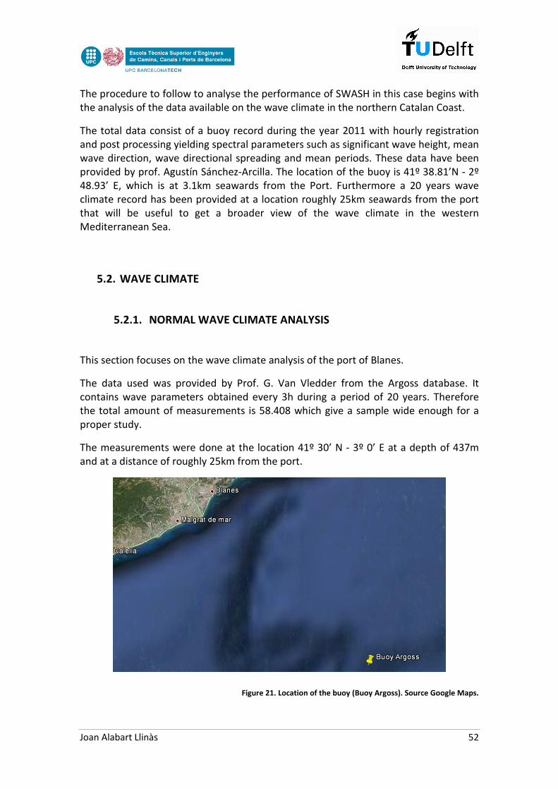
Joan Alabart Llinàs 52
The procedure to follow to analyse the performance of SWASH in this case begins with the analysis of the data available on the wave climate in the northern Catalan Coast.
The total data consist of a buoy record during the year 2011 with hourly registration and post processing yielding spectral parameters such as significant wave height, mean wave direction, wave directional spreading and mean periods. These data have been provided by prof. Agustín Sánchez-Arcilla. The location of the buoy is 41º 38.81’N - 2º 48.93’ E, which is at 3.1km seawards from the Port. Furthermore a 20 years wave climate record has been provided at a location roughly 25km seawards from the port that will be useful to get a broader view of the wave climate in the western Mediterranean Sea.
5.2. WAVE CLIMATE
5.2.1. NORMAL WAVE CLIMATE ANALYSIS
This section focuses on the wave climate analysis of the port of Blanes.
The data used was provided by Prof. G. Van Vledder from the Argoss database. It contains wave parameters obtained every 3h during a period of 20 years. Therefore the total amount of measurements is 58.408 which give a sample wide enough for a proper study.
The measurements were done at the location 41º 30’ N - 3º 0’ E at a depth of 437m and at a distance of roughly 25km from the port.
Figure 21. Location of the buoy (Buoy Argoss). Source Google Maps.
Joan Alabart Llinàs 53
The first step to analyse the wave climate consisted of the creation of the wave rose during this 20 years period. This was done using the WIND_ROSE.mat script (see Annex 2). The results shown in Figure 22 give per each wind direction (each sector) the probability of occurrence for each wave height.
From the previous figure it can be seen that in deep waters the dominant wave directions are from the NE and SW. However it is from the east where the higher waves come from. These eastern storms are of great importance in the north catalan coast and receive the name of “Llevantades”.
The second important parameter when it comes to the wave climate is the significant wave height distribution (Hm0 as it comes from spectral data). This is shown in the following figure:
Figure 23. Hm0 density distribution. Source Argoss database.
0
0.1
0.2
0.3
0.4
0.5
0.5
0
1.0
0
1.5
0
2.0
0
2.5
0
3.0
0
3.5
0
4.0
0
4.5
0
5.0
0
5.5
0
6.0
0
6.5
0
7.0
0
7.5
0
f(x)
Hs (m)
Hm0 density distribution
Figure 22. Wave rose 20year record. Source Argoss database.
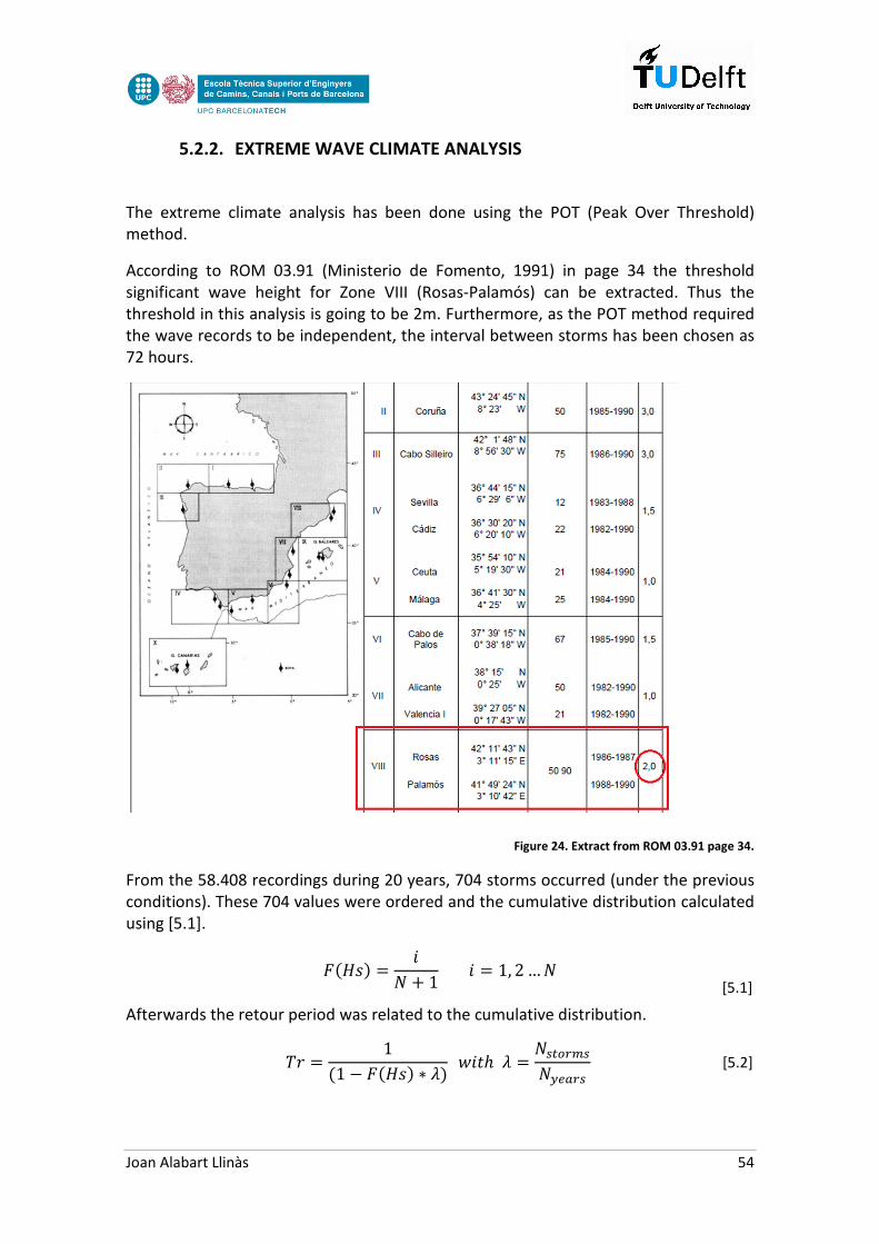
Joan Alabart Llinàs 54
[5.2]
[5.1]
5.2.2. EXTREME WAVE CLIMATE ANALYSIS
The extreme climate analysis has been done using the POT (Peak Over Threshold) method.
According to ROM 03.91 (Ministerio de Fomento, 1991) in page 34 the threshold significant wave height for Zone VIII (Rosas-Palamós) can be extracted. Thus the threshold in this analysis is going to be 2m. Furthermore, as the POT method required the wave records to be independent, the interval between storms has been chosen as 72 hours.
Figure 24. Extract from ROM 03.91 page 34.
From the 58.408 recordings during 20 years, 704 storms occurred (under the previous conditions). These 704 values were ordered and the cumulative distribution calculated using [5.1].
^��;� � ?� � 1 ? � 1, 2…�
Afterwards the retour period was related to the cumulative distribution.
1Y � 1�1 � ^��;� ∗ Ý� !?��Ý � �U�Nc�U�>n�cU
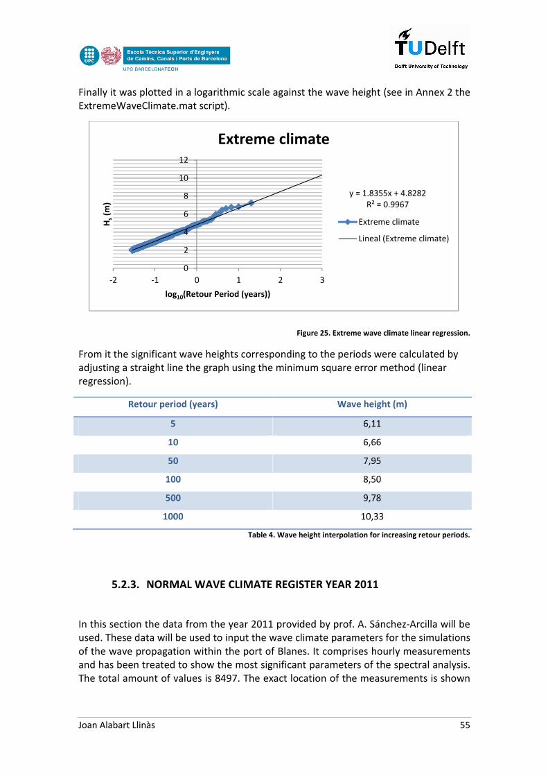
Joan Alabart Llinàs 55
Finally it was plotted in a logarithmic scale against the wave height (see in Annex 2 the ExtremeWaveClimate.mat script).
Figure 25. Extreme wave climate linear regression.
From it the significant wave heights corresponding to the periods were calculated by adjusting a straight line the graph using the minimum square error method (linear regression).
Retour period (years) Wave height (m)
5 6,11
10 6,66
50 7,95
100 8,50
500 9,78
1000 10,33
Table 4. Wave height interpolation for increasing retour periods.
5.2.3. NORMAL WAVE CLIMATE REGISTER YEAR 2011
In this section the data from the year 2011 provided by prof. A. Sánchez-Arcilla will be used. These data will be used to input the wave climate parameters for the simulations of the wave propagation within the port of Blanes. It comprises hourly measurements and has been treated to show the most significant parameters of the spectral analysis. The total amount of values is 8497. The exact location of the measurements is shown
y = 1.8355x + 4.8282R² = 0.9967
0
2
4
6
8
10
12
-2 -1 0 1 2 3
Hs
(m)
log10(Retour Period (years))
Extreme climate
Extreme climate
Lineal (Extreme climate)
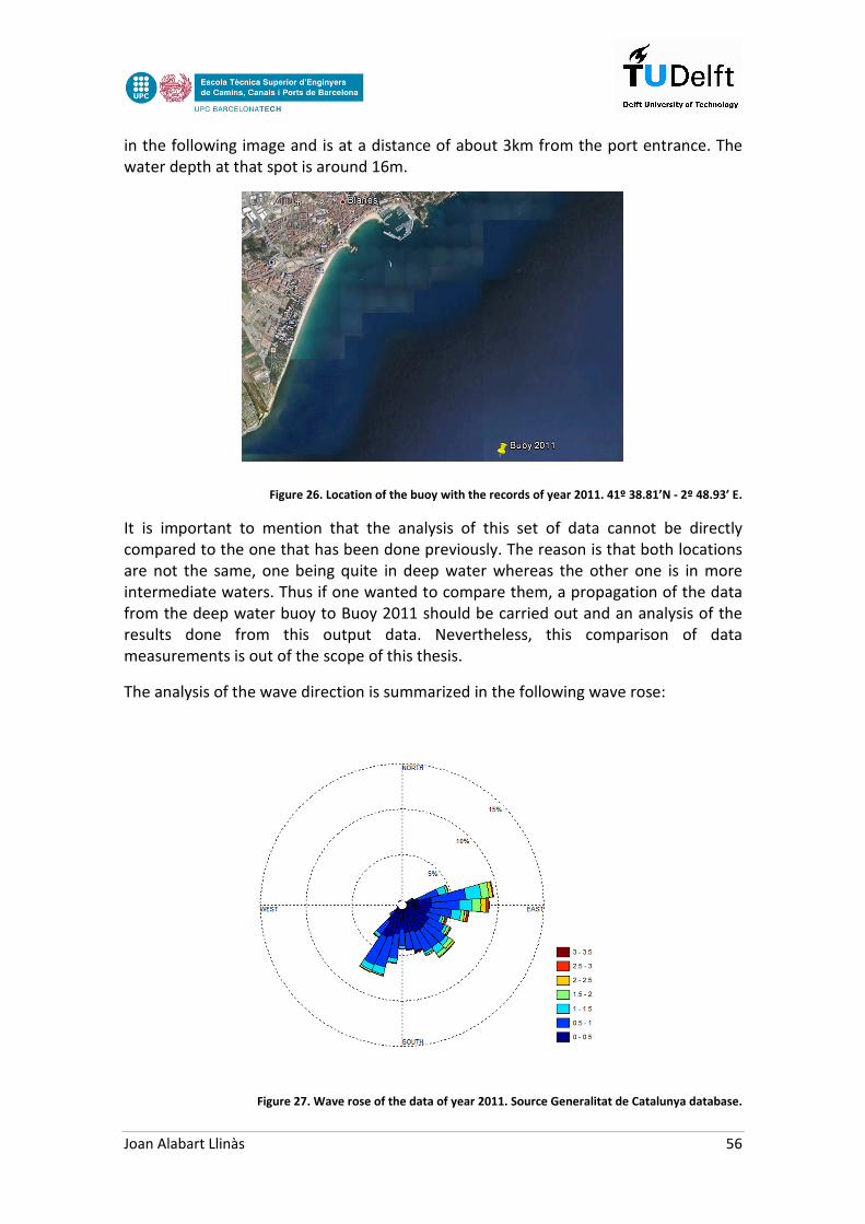
Joan Alabart Llinàs 56
in the following image and is at a distance of about 3km from the port entrance. The water depth at that spot is around 16m.
Figure 26. Location of the buoy with the records of year 2011. 41º 38.81’N - 2º 48.93’ E.
It is important to mention that the analysis of this set of data cannot be directly compared to the one that has been done previously. The reason is that both locations are not the same, one being quite in deep water whereas the other one is in more intermediate waters. Thus if one wanted to compare them, a propagation of the data from the deep water buoy to Buoy 2011 should be carried out and an analysis of the results done from this output data. Nevertheless, this comparison of data measurements is out of the scope of this thesis.
The analysis of the wave direction is summarized in the following wave rose:
Figure 27. Wave rose of the data of year 2011. Source Generalitat de Catalunya database.
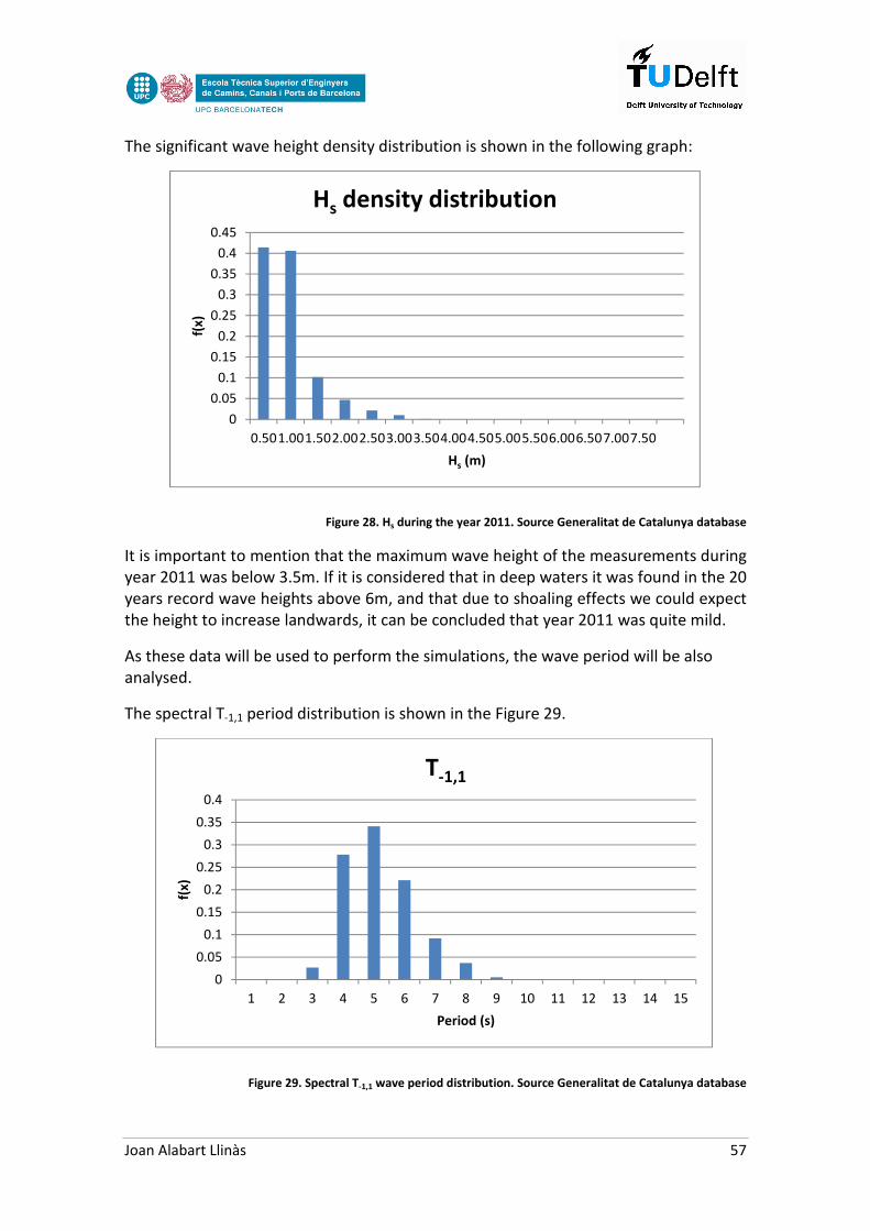
Joan Alabart Llinàs 57
The significant wave height density distribution is shown in the following graph:
Figure 28. Hs during the year 2011. Source Generalitat de Catalunya database
It is important to mention that the maximum wave height of the measurements during year 2011 was below 3.5m. If it is considered that in deep waters it was found in the 20 years record wave heights above 6m, and that due to shoaling effects we could expect the height to increase landwards, it can be concluded that year 2011 was quite mild.
As these data will be used to perform the simulations, the wave period will be also analysed.
The spectral T-1,1 period distribution is shown in the Figure 29.
Figure 29. Spectral T-1,1 wave period distribution. Source Generalitat de Catalunya database
0
0.05
0.1
0.15
0.2
0.25
0.3
0.35
0.4
0.45
0.501.001.502.002.503.003.504.004.505.005.506.006.507.007.50
f(x)
Hs (m)
Hs density distribution
0
0.05
0.1
0.15
0.2
0.25
0.3
0.35
0.4
1 2 3 4 5 6 7 8 9 10 11 12 13 14 15
f(x)
Period (s)
T-1,1
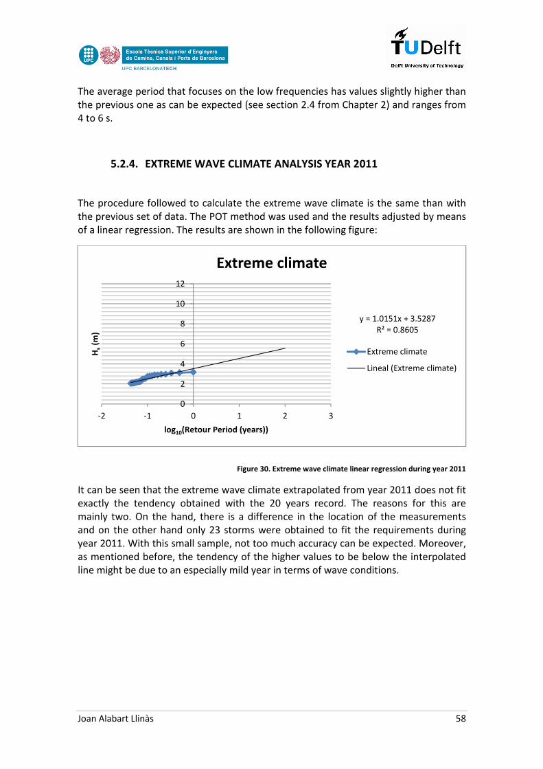
Joan Alabart Llinàs 58
The average period that focuses on the low frequencies has values slightly higher than the previous one as can be expected (see section 2.4 from Chapter 2) and ranges from 4 to 6 s.
5.2.4. EXTREME WAVE CLIMATE ANALYSIS YEAR 2011
The procedure followed to calculate the extreme wave climate is the same than with the previous set of data. The POT method was used and the results adjusted by means of a linear regression. The results are shown in the following figure:
Figure 30. Extreme wave climate linear regression during year 2011
It can be seen that the extreme wave climate extrapolated from year 2011 does not fit exactly the tendency obtained with the 20 years record. The reasons for this are mainly two. On the hand, there is a difference in the location of the measurements and on the other hand only 23 storms were obtained to fit the requirements during year 2011. With this small sample, not too much accuracy can be expected. Moreover, as mentioned before, the tendency of the higher values to be below the interpolated line might be due to an especially mild year in terms of wave conditions.
y = 1.0151x + 3.5287R² = 0.8605
0
2
4
6
8
10
12
-2 -1 0 1 2 3
Hs
(m)
log10(Retour Period (years))
Extreme climate
Extreme climate
Lineal (Extreme climate)
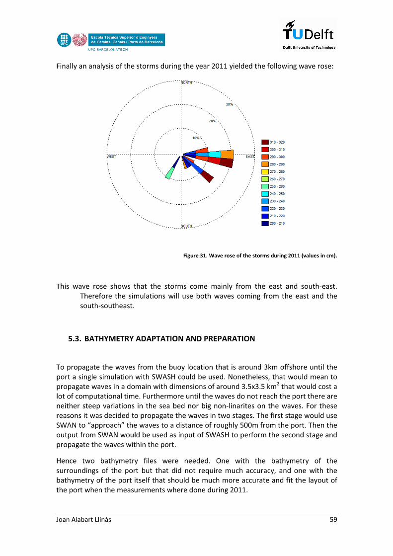
Joan Alabart Llinàs 59
Finally an analysis of the storms during the year 2011 yielded the following wave rose:
Figure 31. Wave rose of the storms during 2011 (values in cm).
This wave rose shows that the storms come mainly from the east and south-east. Therefore the simulations will use both waves coming from the east and the south-southeast.
5.3. BATHYMETRY ADAPTATION AND PREPARATION
To propagate the waves from the buoy location that is around 3km offshore until the port a single simulation with SWASH could be used. Nonetheless, that would mean to propagate waves in a domain with dimensions of around 3.5x3.5 km2 that would cost a lot of computational time. Furthermore until the waves do not reach the port there are neither steep variations in the sea bed nor big non-linarites on the waves. For these reasons it was decided to propagate the waves in two stages. The first stage would use SWAN to “approach” the waves to a distance of roughly 500m from the port. Then the output from SWAN would be used as input of SWASH to perform the second stage and propagate the waves within the port.
Hence two bathymetry files were needed. One with the bathymetry of the surroundings of the port but that did not require much accuracy, and one with the bathymetry of the port itself that should be much more accurate and fit the layout of the port when the measurements where done during 2011.

Joan Alabart Llinàs 60
Even though prof. A. Sánchez-Arcilla tried to provide the bathymetry of the new layout of the port, it was not possible and the bathymetry that was provided corresponded to the old layout. This was an issue because the measurements from year 2011 were done when the port was already expanded and therefore there was a mismatch on the bathymetries. The bathymetry that was provided is shown in Figure 32.
Figure 32. Scatter plot of the data provided from the old bathymetry
That corresponded to the location shown in this plan view of the port.
Figure 33. Plan view of the domain included in the old bathymetry
Two further complications could be observed. On the one hand the data was provided as a set of XUTM-YUTM-Depth coordinates instead of a matrix. On the other hand, the axes that were used when collecting the data were not North-East. Therefore the axes needed to be turned, and a matrix with the water depth from a dx=dy=1m grid created interpolating from the closer values from the provided bathymetry.

Joan Alabart Llinàs 61
100 200 300 400 500 600 700
100
200
300
400
500
600
700
800 0
2
4
6
8
10
12
This was done and yielded the image on figure 33 for a domain of 700x800 m2, the outer breakwater had already been removed.
The next step was to include the new structures. This was done by defining polygons with Matlab. There was a mismatch between the coordinates provided with the old bathymetry and the coordinates extracted from the Cartographic Institute of Catalonia. Thus a shift was done to fit them. Moreover, the mould breakwater was modelled as a 1V 1H sloping structure and the result was:
Figure 34. Old bathymetry adapted. The colours indicate the water depth (left).
Figure 35. New bathymetry adapted from the old one. The colours indicate the water depth (right).
Further improvements in the accuracy of the bathymetry could be carried out but it was seen that rather than modelling the structures as variations in the bottom file, including them as porous structures yielded a much more reliable result. In the end 300m were added at both sides of the port to include wide porous layers to dissipate the waves.
When it comes to the bathymetry in the surroundings of the port to be inputted in SWAN, prof. G. Van Vledder provided data obtained from the Admiralty Charts database. This data base includes charts with different grades of accuracy and reliability. For this reason a routine was used to go over all the different available charts in the surroundings of the port of Blanes, and obtain the most accurate bathymetry.
Figure 36. Aerial view of the adapted bathymetry

Joan Alabart Llinàs 62
This bathymetry was obtained for a domain ranging from 2.75º to 2.85º E and from 41.6º to 41.7º N with an accuracy of 0.0005º in both directions. That is a grid size of dx=42m and dy=56m. The bathymetry file is shown in the following figure where a submarine canyon can be seen in the lower right corner with water depths higher than 500m.
Figure 37. Bathymetry in the surroundings of Blanes. Source Admiralty Charts database.
20 40 60 80 100 120 140 160 180 200
20
40
60
80
100
120
140
160
180
200
0
20
40
60
80
100
120
140
160
180
200
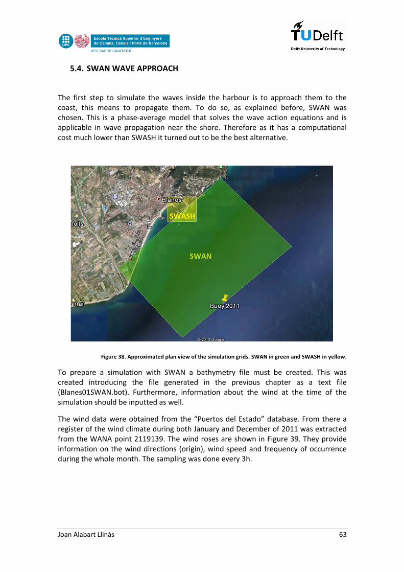
Joan Alabart Llinàs 63
5.4. SWAN WAVE APPROACH
The first step to simulate the waves inside the harbour is to approach them to the coast, this means to propagate them. To do so, as explained before, SWAN was chosen. This is a phase-average model that solves the wave action equations and is applicable in wave propagation near the shore. Therefore as it has a computational cost much lower than SWASH it turned out to be the best alternative.
Figure 38. Approximated plan view of the simulation grids. SWAN in green and SWASH in yellow.
To prepare a simulation with SWAN a bathymetry file must be created. This was created introducing the file generated in the previous chapter as a text file (Blanes01SWAN.bot). Furthermore, information about the wind at the time of the simulation should be inputted as well.
The wind data were obtained from the “Puertos del Estado” database. From there a register of the wind climate during both January and December of 2011 was extracted from the WANA point 2119139. The wind roses are shown in Figure 39. They provide information on the wind directions (origin), wind speed and frequency of occurrence during the whole month. The sampling was done every 3h.

Joan Alabart Llinàs 64
In addition as the storms that wanted to be simulated were a storm from the 16th of December that came from the south-west and a storm from the 28th of January coming from the East, the wind data for these specific days was also extracted from the database.
These values were: for the storm of the 16th of December wind speeds of Vx=12.4m/s and Vy=8.4m/s. For the storm of the 28th of January Vx=-15m/s and Vy=0m/s where the X axis points to the East and the Y axis to the North.
The computational grid had dimensions of 5000x3000 m2 and a spacing of 10m in each direction; in addition it was tilted 46º to be as parallel as possible to the coast. The waves were propagated from 41°38'45.19"N 2°48'54.00"E (the offshore buoy) to 41°40'9.73"N 2°47'52.29"E (were the SWASH simulation would start later).
The wave climate was inputted using a JONSWAP spectrum with the peak period and the dispersion in degrees. The computational time was 1h and the initial time step 0.1s though SWAN adapts it while running the computation depending upon the Courant number. The input files can be found in Annex 1 with all the other input parameters that were considered such as wave breaking, friction, triads and other features.
The first simulation that was done was the simulation of the 16th of December of 2011 at 13h.
The wave input for this simulation was: Hm0=2.54m; Tp=7.1s; θ=58º (from the East counter-clockwise) and a dispersion of 18º (see file Blanes01SWAN.swn in Annex 1). The result is shown in the following graph where the significant wave height is plotted.
Figure 39. Wind roses near Blanes. January (left) and December (right). Source: Puertos del Estado database

Joan Alabart Llinàs 65
Figure 40. Hsig output map from the simulation of the 16/12/2011 at 13h with SWAN
It can be seen that SWAN has some problems with diffraction and some reflection is occurring along the shoreline. Anyway the results at the chosen location were quite realistic and were:
Depth = 16.34m; Hs = 1.58m; Tp = 7.06s; Dspr = 13.53º and θ = 80º.
5.5. SWASH WAVE PROPAGATION WITHIN THE PORT
The second step consisted on the actual simulation with SWASH inputting the results obtained with this simulation with SWAN (see file Blanes01SWASH.sws in Annex 1).
Two options were considered for this simulation.
On the one hand, the port structures could be simulated as variations of the bottom and thus no porosity files would be needed. On the other hand, the bottom could be smoothed, and the structures inputted in the porosity file.
The first option was considered and tested with a grid size of 4m. The results are shown in Figure 41.
50 100 150 200 250 300 350 400 450 500
50
100
150
200
250
300
0.5
1
1.5
2
2.5
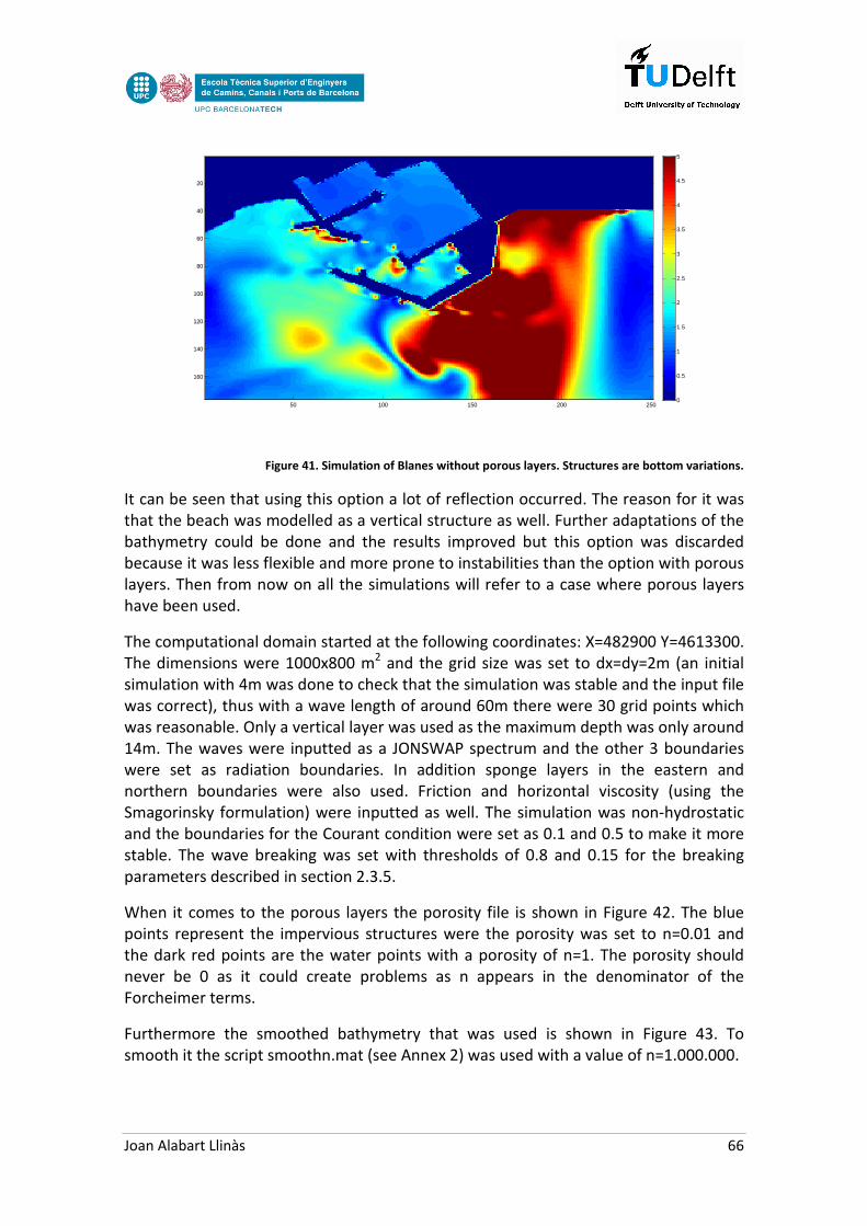
Joan Alabart Llinàs 66
Figure 41. Simulation of Blanes without porous layers. Structures are bottom variations.
It can be seen that using this option a lot of reflection occurred. The reason for it was that the beach was modelled as a vertical structure as well. Further adaptations of the bathymetry could be done and the results improved but this option was discarded because it was less flexible and more prone to instabilities than the option with porous layers. Then from now on all the simulations will refer to a case where porous layers have been used.
The computational domain started at the following coordinates: X=482900 Y=4613300. The dimensions were 1000x800 m2 and the grid size was set to dx=dy=2m (an initial simulation with 4m was done to check that the simulation was stable and the input file was correct), thus with a wave length of around 60m there were 30 grid points which was reasonable. Only a vertical layer was used as the maximum depth was only around 14m. The waves were inputted as a JONSWAP spectrum and the other 3 boundaries were set as radiation boundaries. In addition sponge layers in the eastern and northern boundaries were also used. Friction and horizontal viscosity (using the Smagorinsky formulation) were inputted as well. The simulation was non-hydrostatic and the boundaries for the Courant condition were set as 0.1 and 0.5 to make it more stable. The wave breaking was set with thresholds of 0.8 and 0.15 for the breaking parameters described in section 2.3.5.
When it comes to the porous layers the porosity file is shown in Figure 42. The blue points represent the impervious structures were the porosity was set to n=0.01 and the dark red points are the water points with a porosity of n=1. The porosity should never be 0 as it could create problems as n appears in the denominator of the Forcheimer terms.
Furthermore the smoothed bathymetry that was used is shown in Figure 43. To smooth it the script smoothn.mat (see Annex 2) was used with a value of n=1.000.000.
50 100 150 200 250
20
40
60
80
100
120
140
160
0
0.5
1
1.5
2
2.5
3
3.5
4
4.5
5

Joan Alabart Llinàs 67
Figure 42. Porosity file. The porosity is n=0.01 for the port structures and 1 in the rest
Figure 43. Smoothed bathymetry using n=1.000.000.
Finally, the upwind first order discretization was used for the momentum equations (i.e. UMOM and WMOM) and the correction in the velocity points equation (i.e. CORRDEP) to make it stable as was explained in Chapter 4.
The simulation time was 20 minutes and the HRMS output map was created during the last 10 minutes of simulation. With this setting the simulation took 4h 15min with a normal laptop. If the accuracy were to be improved to dx=dy=1m or several vertical layers were used, it is recommendable to use a cluster with several processors and run SWASH in the parallel mode.
100 200 300 400 500 600 700 800 900 1000
100
200
300
400
500
600
700
800 0.1
0.2
0.3
0.4
0.5
0.6
0.7
0.8
0.9
1
100 200 300 400 500 600 700
100
200
300
400
500
600
700
800 0
2
4
6
8
10
12

Joan Alabart Llinàs 68
50 100 150 200 250 300 350 400 450 500
50
100
150
200
250
300
350
400 0
0.2
0.4
0.6
0.8
1
1.2
1.4
1.6
1.8
2
50 100 150 200 250 300 350 400 450 500
50
100
150
200
250
300
350
400 0
0.1
0.2
0.3
0.4
0.5
0.6
0.7
0.8
0.9
1
The HRMS output map is shown in Figure 44. In the first graph the waves range from +2m (red) to 0m (dark blue). In the second graph the range is from +1m to 0m to be able to visualize better the penetration of the waves inside the port.
It can be seen that the results are realistic. First of all, a standing wave pattern can be observed in front of the breakwaters. The reason for it is that they have been modelled as almost impervious structures. In addition it can be seen that the two “beaches” and sponge layers located next to the port do dissipate the waves correctly. Furthermore, it can be seen that waves enter the port due to diffraction and spread along the different basins. A certain standing wave pattern can be seen also inside the port because of the reflection against the inner structures even though as the waves are irregular is quite smoothed and not steady as the waves are irregular.
The other set of cases that wanted to be analysed were the storms coming from the east occurring mainly during January 2011. The first case that was simulated was the storm from the 28th of January of 2011 at 01h that had a wave record in the offshore buoy of Hs=2.78m; Tp=6.6s, θ=158º (from the east counter-clockwise) and dispersion
Figure 44. HRMS map from the Port of Blanes. Upper figure with the colours going from 0 to 2m. Lower figure with the colours going from 0 to 1m for more accuracy within the port.

Joan Alabart Llinàs 69
100 200 300 400 500 600
50
100
150
200
250
300
350
400 0
0.2
0.4
0.6
0.8
1
1.2
1.4
1.6
1.8
2
100 200 300 400 500 600
50
100
150
200
250
300
350
400 0
0.1
0.2
0.3
0.4
0.5
0.6
0.7
0.8
0.9
1
of 33º. The output of the simulation Blanes02SWAN.swn (see Annex 3) yielded the following parameters that were inputted in the SWASH simulation: Hs=2.32m; Tp=6.63s; θ=150º and dispersion of 26.4º. The computational grid was set similarly to the case with the waves coming from the south with the only difference that the domain was increased 200m in the left boundary to include a sponge layer that could dissipate the waves reaching the western boundary. The results are shown in Figure 45.
It can be seen that the wave penetration inside the harbour is much smaller than with the waves coming from the south. This makes sense as the majority of the storms come from the east, south-east, therefore the entrance to the port faces the west to minimize the wave penetration inside the port. A standing wave pattern can be seen inside the port and in the surroundings because of the reflection of the waves against the structures. Further simulations with similar cases will be explained in the following section from this chapter.
Figure 45. Hrms map from the Port of Blanes. Upper figure with the colours going from 0 to 2m. Lower figure with the colours going from 0 to 1m for more accuracy within the port.

Joan Alabart Llinàs 70
5.6. COMPARISON OF THE RESULTS WITH THE MEASUREMENTS
The final step consisted in the comparison of the results obtained with the real data measured inside the port. This verification was done with two sets of storms. On the one hand, the storm from the 16th of December was used and different hours with slightly different wave climates were inputted in the model to see the different results with small variations in the parameters. On the other hand, the storm of the 28th of January was also used and the same process done.
The buoy inside the port is located in the following place:
Figure 46. Location of the buoy inside the port of Blanes in the frame of the old port. Source ICC.
Nonetheless, it is important to point out that even though the ultimate goal of the thesis was to do this verification and see how accurate SWASH was in harbour domains, some things must be outlined before analysing the results.
- First of all, although the data outside the port is accurate, the location of the measurements inside the port is not utterly known. As a standing wave pattern was seen inside the port, slightly variations of the location of the gauge may create great discrepancies in the results.
- Secondly, SWASH has not been the only model used. If there are some errors, they may be due to either the approach with SWAN or the propagation with SWASH.
- Ultimately, to ensure a stable simulation with SWASH some simplifications have been done. In addition the data available was not accurate enough and therefore some adaptations and assumptions were applied.
Bearing all this in mind, the results between the model and the actual measurements were compared. To overcome the inaccuracy of the buoy inside the port, it was decided to do a mean of the values around the supposed location of the measurements.
The first set of cases corresponded to the records from December 2011 with waves coming from the south and south-west.
Joan Alabart Llinàs 71
Case B011: corresponds to the case that has already been explained from the 16th of December 2011 at 13h.
Case B012: this case corresponds to the 16th of December 2011 at 16h and thus is the same storm than the previous case. The input data for SWAN was: Hs=2.05m; Tp=7.7s; Dispersion= 22º and θ=68º (from the east counter-clockwise). Once the SWAN simulation was done (see results in Annex 3), the input parameters for SWASH were Hs=1.48m; Tp=7.76s, Dispersion=16.5º and θ=87.6º.
Case B013: this case corresponds to the 17th of December 2011 at 03h where the input data for SWAN was: Hs=1.59m; Tp=10s; Dispersion=40º and θ=66º. From it, after the SWAN simulation, the input results for the SWASH simulation were: Hs=1.13m; Tp=10s; Disp=21.6º and θ=169.2º.
The second set of cases correspond to the storms coming from the east during the storm of the 28th and 29th of January 2011.
Case B02: this case corresponds to the storm that occurred the 28th of January 2011 at 01h, the input data for the SWAN simulation were: Hs=2.78m; Tp=6.6s, Disp=33º and θ=158º (the same orientation than the previous ones). The output data of SWAN and thus input parameters for SWASH were: Hs=2.32m; Tp=6.63s; Disp=23.4º and θ=120º.
Case B021: this case corresponds to the storm that occurred the 29th of January 2011 at 20h; this case has been chosen as it has a more extreme orientation (eastwards) of the waves, and a longer period. Then, the input data for the SWAN simulation were: Hs=2.06m; Tp=10s; Disp=23º and θ=197º (the same orientation than the previous ones). The output data of SWAN and thus input parameters for SWASH were: Hs=1.61m; Tp=10s; Disp=16.5º and θ=168.3º.
Case B022: this case corresponds to the storm that occurred the 28th of January 2011 at 21h, this case has been chosen because the wave height is quite high and so is the wave dispersion. Then, the input data for the SWAN simulation were: Hs=2.23m; Tp=10s; Disp=37º and θ=170º (the same orientation than the previous ones). The output data of SWAN and thus input parameters for SWASH were: Hs=1.96m; Tp=10s; Disp=16.5º and θ=168.3º.
The SWASH files for all the results can be found in Annex 1.
To compare the real measurements inside the port during the corresponding days in 2011 and the results of the simulation, an average of the HRMS in the points surrounding the location of the buoy was done, an area of 20x20m2 was considered. Afterwards the HRMS was converted into Hs by using the relations explained in Chapter 2. The comparison between the simulated values and the real data is summarized in the following table:

Joan Alabart Llinàs 72
CASE
HRMS
(SWASH)
Hs
(SWASH) Hs (buoy)
Absolut
error
Relative
error
(cm) (cm) (cm) (cm) (%)
Blanes011 24.54 34.71 42.78 -8.07 18.86
Blanes012 32.39 45.81 34.77 11.04 31.75
Blanes013 19.88 28.11 51.84 -23.73 45.78
Blanes02 13.95 19.72 21.66 -1.94 8.96
Blanes021 2.37 3.35 15.44 -12.09 78.30
Blanes022 8.23 11.64 17.25 -5.61 32.52
Table 5. Comparison between the real measurements and the results of the simulation.
This results show that there are some discrepancies between the predicted results and the actual measured wave heights. These variations can be due to many factors the most important of which can be classified as errors in the data, errors in the simulation with SWAN and errors in the simulation with SWASH.
- The location of the buoy is not exact. As a standing wave pattern occurs in front of the quay where the buoy is located, by doing the mean of the near values to this location an important error may be included. In case the gauge was located in the nodes of the standing wave, by doing the mean the results would have been overestimated. If the buoy was actually in the antinode an underestimation would occur.
- The SWAN simulation can have produced inaccurate results that may be due either to the limitations of the model itself when modelling diffraction and to the simulation that was done doing some simplifications. The most important simplifications that were done by using SWASH were first of all the bathymetry that, even though was obtained from a reliable source, was not accurate enough. In addition the boundary conditions acting as wave generators in some cases could be another source of errors. Also the orientation of the grid in some cases were it did not match the wave direction could have been another source of error.
- The simulation with SWASH was done by simplifying the reality to make it feasible to be simulated. This simplification included the suppression of the topography in the surroundings of the port that was substituted for dissipative beaches, the consideration of the port structures as impervious layers without accounting for the mound breakwater. In addition the small beach for landing of small boats that was located within the port was somehow suppressed. It is important to mention as well that the bathymetry was obtained adapting the old bathymetry and ultimately smoothed to help improve the stability of the simulation. Furthermore when the wave climate was too eastwards oriented the computational domain was not totally appropriate as only the southern boundary acted as a generator of waves. In such a case diffraction towards
Joan Alabart Llinàs 73
shadow areas may have diminished considerably the energy that actually entered the port.
All these factors may have produced errors in the simulation and therefore the comparison between the real measurement and the output data of the simulation should not be taken too much into account. Measures to improve further simulations, recommendations and conclusions will be drawn in Chapter 6.
Joan Alabart Llinàs 74
CHAPTER 6: CONCLUSIONS AND RECOMMENDATIONS
In this chapter the results of this thesis will be analysed by pointing out and explaining the recommendations for further work on this field and the conclusions that can be drawn from the initial question of the thesis that was:
- Is SWASH a useful tool to simulate the propagation of waves in harbour domains?
6.1. CONCLUSIONS
The main conclusion of this thesis is that SWASH is indeed an extremely valuable tool to simulate the propagation of waves in port domains. The reason for it is that it is capable of simulating almost all the phenomena that occur in shallow waters with environments where the properties vary rapidly. It generates realistic results and even though in this thesis it has not been totally possible to prove so, the author is confident that the results are accurate as well if the data inputted is accurate enough. However, as this model is still in the early phases of development it still has some bugs and limitations. Nonetheless, with the actual version 1.20 it has been proved that this model is capable of dealing with complex two-dimensional cases yielding realistic results.
6.2. RECOMMENDATIONS
This section will focus on all the ideas that have arisen while developing this thesis that could help in the future to spread this model and to become the cornerstone of harbour design when it comes to wave agitation within the ports.
Recommendations for the developers of the model: The first suggestion is to make SWASH more user-friendly. The reason for this is that it takes time to learn how to use it unless the user is acquaint with previous models such as SWAN. Thus the implementation of an interphase were the user could input easily the different settings and parameters would definitely help to spread the model. Furthermore, nowadays a post processing of the results using other tools like Matlab is necessary. The implementation of a version where the plots of the required output parameters were done if requested by the user would also help to make it more user-friendly.
Secondly when it comes to the model itself it still has some lacks. The first one is that the input data in the boundary condition is the same for all the boundary condition. This means that although the water depth is different the inputted waves have the
Joan Alabart Llinàs 75
same characteristics. This may not be a problem in a perfect case where the waves travel perpendicular to a boundary condition and the slope of the bottom is gradual but in reality this seldom happens. This can be clearly seen in case Blanes021 (see results in Annex 3) where the waves came with a sharp angle with the boundary condition but due to this problem the eastern boundary was not used as a generator of waves as it would lead to unrealistic results.
Another important factor to improve in SWASH is the way it models breakwaters. Nowadays the input parameters are the structure height, the porosity and the grain size apart from the Forchheimer α and β parameters. These parameters are the same for each layer in the same spot and thus it is not possible to model properly a mould breakwater as SWASH calculates a mean value of the porosity depending on the height of the structure, the porosity and the water depth and applies this value in all the layers. A suggestion to overcome this problem could be to input the values of the parameters for each layer, or in case the height of the structure was less than the water depth, to consider different values for the different layers. This is in essence to use different input parameters for the different layers. In addition to this, the Forchheimer dissipative terms should also be included in the vertical momentum equation as (Mellink, 2012) suggested. With this a sloping porous structure would be reproduced in a more realistic way.
Recommendations for the validation of the model with a real case: To be able to validate the model and calibrate the parameters it is suggested to obtain accurate data of a port, with measurements in certain and utterly known spots. This mainly concerns to the procurement of an accurate bathymetry, accurate measurements near the port (where it is not necessary to use SWAN to approximate the waves) and accurate measurements inside the port.
Recommendations for the application of SWASH in harbour domains: To use SWASH in harbour domains it is suggested to use the first order discretization scheme that has been explained in this thesis to ensure the stability of the model. In addition to model the harbour structures the use of porous layers seems the best option as it is more flexible and stable than steep changes of the bathymetry. It is also suggested to start simple and obtain sea level maps every 1s or so and create short movies after the simulations to see how SWASH is performing and if there is something wrong be able to detect it. In case everything looks al right add features until the simulation is as close as possible to the reality. For real wave climates it is suggested to start with a grid size of 4m, see that the simulation is stable and the results realistic and then decrease the grid size to 2 or 1m depending on the accuracy required and the computational power available. In the boundaries where the waves leave the domain it is suggested to include sponge layers of at least 200-300m width (depending upon the wave direction and waves characteristics) to dissipate them. It is also recommendable to keep in mind what is the goal of the simulation. This means that if
Joan Alabart Llinàs 76
the objective is to assess the downtime inside a port, the features of the coast outside the port, as long as they do not affect the propagation of the waves inside the port, do not need a great accuracy as the results would be the same in the desired domain. Furthermore when it comes to the assessment of the navigability of the approach channels, SWASH does not yet provide the instant wave direction. Nevertheless, outputting the instant water velocities and accelerations the wave direction can be obtained.

Joan Alabart Llinàs 77
CHAPTER 7: REFERENCES
[1] Anthoni, J. F. (2000). Oceanography: waves. Theory and principles of waves, how they work and what causes them.
[2] Battjes. (1994). Shallow Water Wave Modelling. Paper presented at the International
Symposium: Waves Physical and Numerical Modeling, University of bristish Columbia, Vancouver.
[3] Booij, N., Ris, R. C., & Holthuijsen, L. H. (1999). A third-generation wave model for coastal
regions 1. Model description and validation. J. Geophys. Res., 104(C4), 7649-7666. doi: 10.1029/98jc02622
[4] Bosboom, J., & Stive, M. J. F. (2013). Coastal Dynamics I. Delft University of Technology.
[5] Burcharth, H. F., & Andersen, O. K. (1995). On the one-dimensional steady and unsteady
porous flow equations. Coastal Engineering, 24(3-4), 233-257. [6] Cavaleri, L., & Malanotte-Rizzioli, P. (1981). Wind wave prediction in shallow water: Theory
and applications. J. Geophysics. [7] Collins, J. I. (1972). Prediction of shallow wate spectra. J. Geophysics. [8] Daemrich, K.-F., & Kohlhase, S. (2011). INFLUENCE OF BREAKWATER-REFLECTION ON
DIFFRACTION.
[9] Dean, R. G., & Dalrymple, R. A. (1984). Water Wave Mechanics for Engineers and Scientist
(Vol. 2).
[10] Fenton, J. (2010). Coastal and Ocean Engineering. TU Wien, Institut für Wasserbau und
Ingenieurhydrologie.
[11] Guzmán, C. (2011). Impact of access channel geometry on wave penetration in harbours.
TU Delft. [12] Kinsman. (1984). Surface gravity waves scheme.
[13] Kuik, A. J., Vledder, G. V., & Holthuijsen, L. H. (1988). A Method for the Routine Analysis of
Pitch-and-Roll Buoy Wave Data. Journal of Physical Oceanography. [14] Ligteringen, H., & Velsink, H. (2012). Ports and Terminals. Delft: VSSD.

Joan Alabart Llinàs 78
[15] Mellink, B. (2012). Numerical and experimental research of wave interaction with a porous
breakwater. TU Delft. [16] Miche, R. (1944). Mouvement ondulatoires de la mer en profondeur contante ou
decroissante Annales des Ponts et Chaussees. [17] Ministerio de Fomento, G. d. E. (1991). ROM 0.3-91 Recomendación para Oleaje y Atlas de
Clima Marítimo en Litoral español.
[18] Nwogu, O. G., & Demirbilek, Z. (2001). BOUSS-2D: A Boussinesq Wave Model for Coastal
Regions and Harbors: US Army Corps of Engineers.
[19] Penney, W. G., & Price, A. T. (1952). Part I. The Diffraction Theory of Sea Waves and the
Shelter Afforded by Breakwaters. Philosophical Transactions of the Royal Society of
London. Series A, Mathematical and Physical Sciences, 244(882), 236-253. doi: 10.1098/rsta.1952.0003
[20] Polubarinova-Kocina, P. J. (1962). Theory of ground water movement. Princeton, NJ: Univ.
Pr.
[21] R.Boshek, M. (2009). Reflection and Diffraction Around Breakwaters. TU Delft, Delft. [22] Randall, D. A. (2006). The Shallow Water Equations. Retrieved from [23] U.S.Army_Corps_of_Engineers. (2002). The Coastal Engineering Manual, Document EM
1110-2-1100, U.S. Army Corps of Engineers (Vol. volume 2). Washington, D.C.: U.S. Army Corps of Engineers.
[24] Van Gent, M. R. A. (1992). Formulae to describe porous flow (C. E. a. Geosciences, Trans.)
Communications on hydraulic and geotechnical engineering, No. 1992-02.
[25] Walkley, M. A. (1999). A Numerical Method for Extended Boussinesq Shallow-Water Wave
Equations. The University of Leeds School of Computer Studies. [26] Wikipedia. from http://en.wikipedia.org/wiki/Airy_wave_theory
[27] Zijlema, M., & Stelling, G. S. (2008). Efficient computation of surf zone waves using
nonlinear shallow water equations with non-hydrostatic pressure. Coastal Engineering,
55.