maestrÍa en valuaciÓn ... - infonavit.janium.net · mayor solidez a su opinión de valor, ... 3.1...
TRANSCRIPT
i< ITC #"«<„*., „i 4 ; » , *í> I» « ¡ " " f e •SCÍÍWloaUít is«^|.?í»*^«í«>\v i.tr ¿isle's I * '•*» £*»»&ífiKíI¡JíS
IN5TITUT0 TECNOLÓGICO DE LA CONSTRUCCIÓN
DELEGACIÓN JALISCO
ESTUDIOS CON RECONOCIMIENTO DE VALIDEZ OFICIAL POR PARTE DE LA SECRETARIA DE EDUCACACIÓN PÚBLICA CONFORME AL
ACUERDO RVOE SEP N° 2003368 DE FECHA DE DICIEMBRE DEL 2003
MAESTRÍA EN VALUACIÓN INMOBILIARIA E INDUSTRIAL
"APLICACIÓN DEL MODELO HEDÓNICO EN VALUACIÓN COMERCIAL"
TESIS QUE PRESENTA PARA OBTENER EL GRADO DE MAESTRO EN VALUACIÓN INMOBILIARIA E INDUSTRIAL
ARQUITECTO FRANCISCO JAVIER ACOSTA CARBAJAL
ASESOR
MVI ARQUITECTO JUAN MANUEL BRAVO ARMEJO
GUADALAJARA, JALISCO, JULIO DEL 2008
V>BV>\CATO^\AS Este trabajo de tesis quiero dedicarlo y
ofrecerlo primero que nada a Dios por permitirme la
oportunidad de superarme a través del conocimiento.
A mi Madre, por su ejemplo diario de amor, esfuerzo
constancia y tenacidad, y por alentarme siempre a
superarme y a salir adelante.
A mi Padre, que me ha hecho mucha falta, que por
desgracia se nos adelanto en el camino, pero que nunca ha
dejado de estar al lado mío disfrutando esta maestría.
A mi Teresita compañera en esta aventura y de mi vida.
A mis niños Francisco, Javier y Luis, regalos que Dios que
me dio, espero que en un futuro les sirva de ejemplo.
A mis hermanitas Julieth y Lupita, a mis hermanos
Enrique y Saúl, por su apoyo total, por su amor y
compañerismo.
A Don Raúl y Techi por su compañía, su apoyo y su
confianza.
APLICACIÓN DEL MODELO HBV>ÓN\CO EN VALUACIÓN
AGRADECIMIENTOS Agradezco a todas los maestros, personas e
instituciones que tan amablemente me apoyaron
durante la maestría, as\ como en la realización de este
trabajo, muy en especial a:
M.V.I. ARQ. Juan Manuel Bravo Armejo
M. EN ECONOMÍA Irán Chávez Lagos
M. C. Porfirio Gutiérrez González
C. P. Javier Mathías Medina
ARQ. Luis Rodolfo Ochoa Ramírez
Instituto Tecnológico de la Construcción
Universidad ITESO
APLICACIÓN X>BL MODELO KEDÓNICO 6N VALUACIÓN
(.-INTRODUCCIÓN
La ciudad de Guadalajara desde sus inicios
siempre ha presentado como una de sus
características principales su gran vocación comercial;
ya que al ser un punto estratégico dentro de la
geografía del país, ha permitido el tránsito e
intercambio de mercancías de distintas índoles.
Esta vocación natural que tiene la ciudad le ha
agregado un dinamismo único en la comercialización de
sus bienes, productos y servicios que no se pueden
encontrar en otras ciudades de nuestro país, y que en
el ámbito inmobiliario se manifiesta en la gran oferta,
demanda y variedad de productos o viviendas que se
pueden negociar.
De esta manera el trabajo del Valuador toma una
mayor complicación comparada con la que se
encontraría en un mercado más uniforme y
estandarizado que el de la ciudad de Guadalajara.
Atendiendo a esta inquietud y buscando
alternativas que permitan que el valuador obtenga
herramientas y habilidades para obtener una mayor
aproximación al valor ideal de un bien, se f i jo la tarea
de buscar distintas opciones o metodologías para
lograr este objetivo; descubriendo un método
econométrico que está tomando auge en algunos países
latinoamericanos que se conoce como "Precios
Hedónicos".
6 N ÜEL MODELO HECÓNICO EN VALUACIÓN
Este método, que algunos especialistas
atribuyen al economista Zvi Sriliches y otros a
Sherwin Rosen, plantea como postulado que el valor de
un bien se obtiene a través del valor de sus atributos.
Este concepto que aunque a primera vista
sostiene el mismo principio que se utiliza en los
modelos tradicionales de valuación, permite agregar
atributos o características que poseen los bienes y que
en muchas ocasiones es difícil cuantif¡car en un avalúo
convencional; tales como ubicación frente a un parque,
mejor orientación, mejor proyecto arquitectónico,
calidad de zona urbana, etc.
El análisis de estas características particulares
de cada bien inmueble podría permitir al valuador
identificar y asignar un valor justificado que le daría
mayor solidez a su opinión de valor, y le permitiría
visualizar un panorama mayor en un mercado tan
heterogéneo y dinámico como el de esta ciudad.
APLICACIÓN DEUMODeLO HEE>ÓNICO BN VALUACIÓN
ÍNWce IV.- CALCULO DEL PRECIO HEDÓNICO
5.1.-Segundo paso o cálculo del precio hedónico
INTRODUCCIÓN V.- REALIZACIÓN DE AVALÚOS COMERCIALES
I.- MARCO TEÓRICO VI.- COMPARACIÓN DE RESULTADOS
I I . - ANTECEDENTES
2.1 historia de Jardines del Bosque
V I I . - CONCLUSIONES Y RECOMENDACIONES
VIII.- BIBLIOGRAFÍA
I I I . - OFERTA DE VIVIENDA EN JARDINES DEL
BOSQUE IX.- ANEXOS
3.1 Descripción y definición de las características
analizadas
3.2 Primer paso en la aplicación del modelo hedónico.
APLICACIÓN DEL MODELO HEDÓNICO EN VALUACIÓN
I . -MARCO TEÓRICO
H**$&$4to. :>. ....
*.. * > • * * • * • • , * « < * > . • * * • * *
. '—V .* .í
3** ^ t ^ "
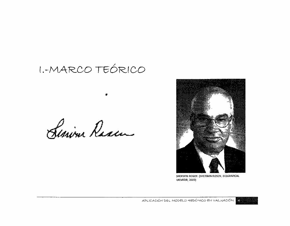
SHERWIN ROSEN (SHERWIN ROSEN, BI0GRAF1CAI MEMOIR, 2003)
APLICACIÓN t>EL MODELO H6I5ÓNICO EN VALUACIÓN

MARCO T8ÓRICO
Es difícil establecer con certeza cuál de los
distintos autores fue el creador del término
"hedónico" en la economía, algunos mencionan a Andrew
Court, como el primero en utilizar este término en el
año de 1939, aunque también se menciona que fue el
economista lituano Zvi Griliches1 el creador de este
modelo; pero debemos aclarar que la siguiente tesis
está basada en la propuesta realizada por el
economista americano Sherwin Rosen que planteó un
modelo de aplicación para los precios hedónicos.
Rosen publico un artículo en "The University of
Chicago Press" en el año de 1974, con el nombre de
1 ("Price Indexes and Quality Change. Stuides in New Methods of Measurement, 1971)
"Hedonic Prices and Implicit Markets: Product
Diferentiation in Pure Competition"2. En este
documento Rosen plantea como principio básico que los
bienes pueden ser valuados por sus atributos o
características.
Es decir, los precios hedónicos son definidos
como los precios implícitos de los atributos, en donde
cada una de las características propias del bien posee
una parte del valor total del mismo, y son revelados a
través de la observación de un grupo específico de
características y de los precios asignados a cada una
de ellas.
Propone como técnica básica el realizar dos
etapas, la primera consiste en aplicar un análisis de
2 (SHERWIN, 1974)
4CIÓN DEL MODELO HEDÓNICO EN VALUACIÓN K f tBi¡iJ¡B8
regresión múltiple del precio de un bien en
relación de cada uno de sus atributos; se calcula la
derivada parcial del precio del bien con respecto a
cada atributo y el resultado se puede interpretar como
un precio marginal implícito. La segunda etapa consiste
en utilizar estos precios implícitos para estimar el
valor del bien en base a las demandas de los atributos.
La teoría de los precios hedónicos esta
formulada como un problema económico de equilibrio
espacial3, en donde los precios implícitos guían tanto al
comprador como al productor en la toma de decisiones.
("A Spatial Equilibrium Model of the Livestock-Feed Economy in the United States", 1953)
Rosen plantea que metodológicamente hablando
se ha demostrado que el conceptual izar un problema de
diferenciación de un producto en base a unas cuantas
características implícitas en vez de una comparación
con bienes genéricos comparables, permite acercar
este análisis a la teoría de la igualación de las
diferencias, también planteada por Rosen y a la
economía de equilibrio espacial.
La teoría de igualación de las diferencias
reconoce que las diferencias básicas pueden ser
requeridas para ecualizar las alternativas atractivas
como las no atractivas de un grupo de estudio.4
Econométricamente los precios implícitos son
estimados por una regresión lineal en donde se analiza
4 ("On the theory of equalizing differences; Increasing abundances of types of workers may increase their earnings", 2001)
JC-ACIÓN DELMOEsELO HBV>ÓNICO EN VALUACIÓN
la relación existente entre una constante "Y" con una
variable independiente "X", pero en el modelo hedónico
se utilizan una cantidad V de variables
independientes o características medibles y objetivas
del bien. De este modo se plantea como una descripción
de equilibrio competitivo en un plano de varias
dimensiones definidas por estas variables
independientes.
Cada una de estas variables es representada por
un vector de coordenadas Z= (Zi, Z2, ... Zn), en donde
el bien es completamente descrito por valores
numéricos de Z y ofrecen a los compradores distintos
paquetes de características.
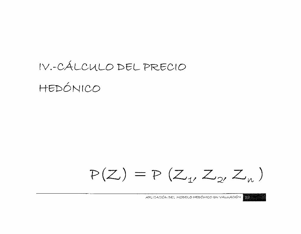
Debido a que el precio del bien se calcula en
base a sus características, se expresa de la siguiente
forma P(Z)= P(Zi, Z2, ...Zn), en donde P(Z) representa
el precio hedónico, P el precio del bien y Zi, Z2, hasta
Zn, representan cada una de las características
analizadas.
La manera de calcular este modelo es a través
de una regresión lineal múltiple en donde se obtiene
una formula expresada de la siguiente forma:
P(Z) = Zi ai +Z2 a2+ Znan+C
1
En donde P(Z) representa el precio hedónico, Zi,
Z n representan cada característica y an representan
cada uno de los "pesos específicos" obtenidos en la
regresión para cada una de las características
investigadas y C representa una constante.
APLICACIÓN P 6 L MODELO HBDONICP ZN VALUACIÓN
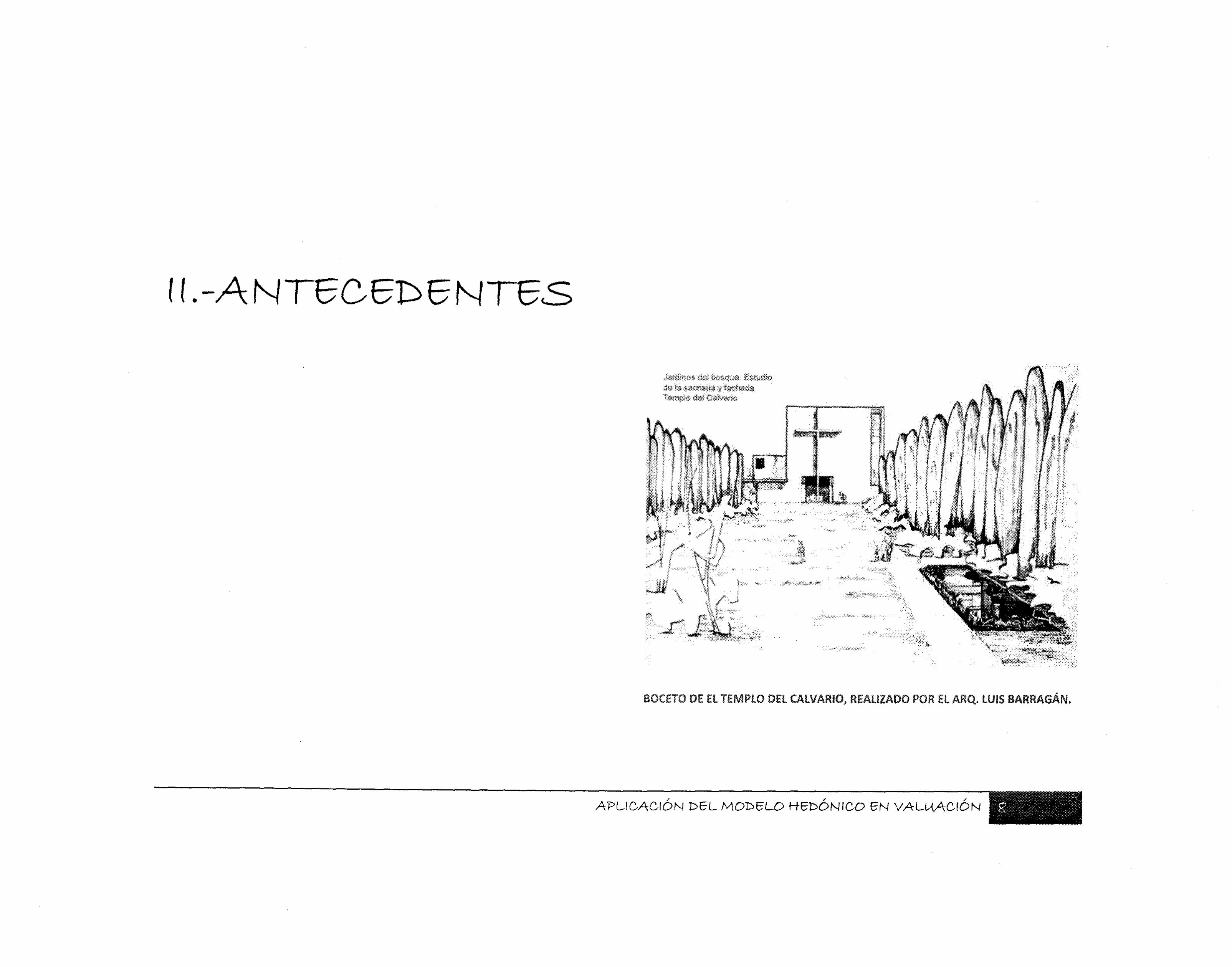
U.-ANTBCS&ENTes,
APLICACIÓN D 6 L MODELO HEDONICO £N VALUACIÓN

Para poner en práctica el modelo hedónico es
necesario recabar información acerca de los bienes
sobre los cuales se busca realizar el estudio.
Para esta tesis se decidió seleccionar una zona
bien determinada en la ciudad de Guadalajara que se
denomina fraccionamiento Jardines del Bosque, ya que
por su mismo desarrollo y ubicación posee diferentes
tipologías de predios y de fincas dentro de un mismo
entorno urbano; además de estar dividida y delimitada
por cinco de las principales avenidas de la ciudad.
*
Esta recolección de datos se inicio en el mes de
enero del 2008 a través de la visita directa a fincas en
proceso de venta para observar las características
consideradas en este estudio.
Cabe mencionar que la información obtenida
representa valores de venta, mas no de operación, ya
que por razones obvias, este valor está sujeto al trato
directo y final entre comprador y vendedor. También
se considero que la información recabada tiene una
validez de un año, en lo referente al precio de venta.
CACIÓN DEL MOtsELO HBX>ÓN\CO EN VALUACIÓN

2 .1 . -H - ISTOR. IA T>B J A R J M N & S t > 6 L
El fraccionamiento Jardines del Bosque fue
construido sobre lo que antes se conocía como el
bosque de Sta. Eduwiges en su primera sección en el
año de 1956, bajo el proyecto del Arq. Luis Barragán.
En este proyecto el arquitecto buscó integrar la
naturaleza del bosque original con el fraccionamiento
al dotar de camellones sus avenidas, sus parques y sus
paseos arbolados.
Con motivo de este proyecto Luis Barragán
mencionó, "Que no nos inquiete modificar la naturaleza
en su condición silvestre si el talento humano tiene la
virtud de poder embellecerla mas y, sobre todo darle
una utilidad para nosotros"5
El fraccionamiento actualmente se divide según
el comité de vecinos y el Ayuntamiento de Guadalajara
en tres secciones definidas como "Sección Centro",
delimitada por las calles de firmamento hacia el
poniente, las avenidas Niños Héroes e Inglaterra al
norte, la Calzada Lázaro Cárdenas hacia el sur y la de
la Av. Mariano Otero hacia el sur6. La "Sección Norte"
quedo delimitada por las Avenida Inglaterra al norte,
la Avenida López Mateos al poniente, la Avenida Niños
5 ("JARDINES DEL BOSQUE" BARRAGAN Y EL HABITAT 1955-2005) 6 ("JARDINES DEL BOSQUE" BARRAGAN Y EL HABITAT 1955-2005, 2005)
ÓN t>EL MOt>ELO HEDÓNICO EN VALUACIÓN HHfl
Héroes al sur y por la Avenida Arcos al oriente7. La
"Sección Sur" o también conocida como "Parque de las
Estrellas" fue la última en urbanizarse en el
fraccionamiento y está delimitada por las Avenidas
Lázaro Cárdenas, Mariano Otero, Las Rosas y
Tonantzin8
El fraccionamiento está asentado sobre una
superficie urbana de 1130,000 m2 aproximadamente
con un inventario aproximado de 6,000 árboles y
115,000 m2 de áreas publicas.9
Debido a su excelente ubicación, a la movilidad
que le otorga tal cantidad de avenidas y a su
7 ("JARDINES DEL BOSQUE" BARRAGAN Y EL HABITAT 1955-2005, 2005) 8 ("JARDINES DEL BOSQUE" BARRAGAN Y EL HABITAT 1955-2005, 2005) 9 ("JARDINES DEL BOSQUE" BARRAGAN Y EL HABITAT 1955-2005, 2005)
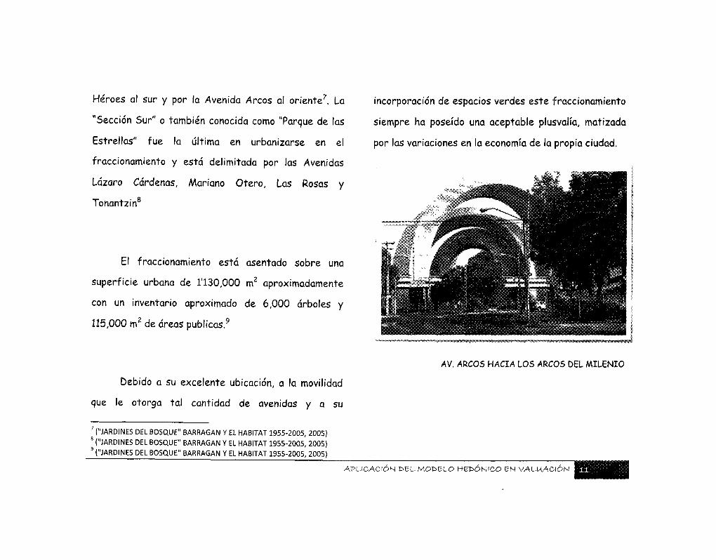
incorporación de espacios verdes este fraccionamiento
siempre ha poseído una aceptable plusvalía, matizada
por las variaciones en la economía de la propia ciudad.
AV. ARCOS HACIA LOS ARCOS DEL MILENIO
¡CACION ÜELMOÜEUO HBt>ON\CO 5N VALUACIÓN
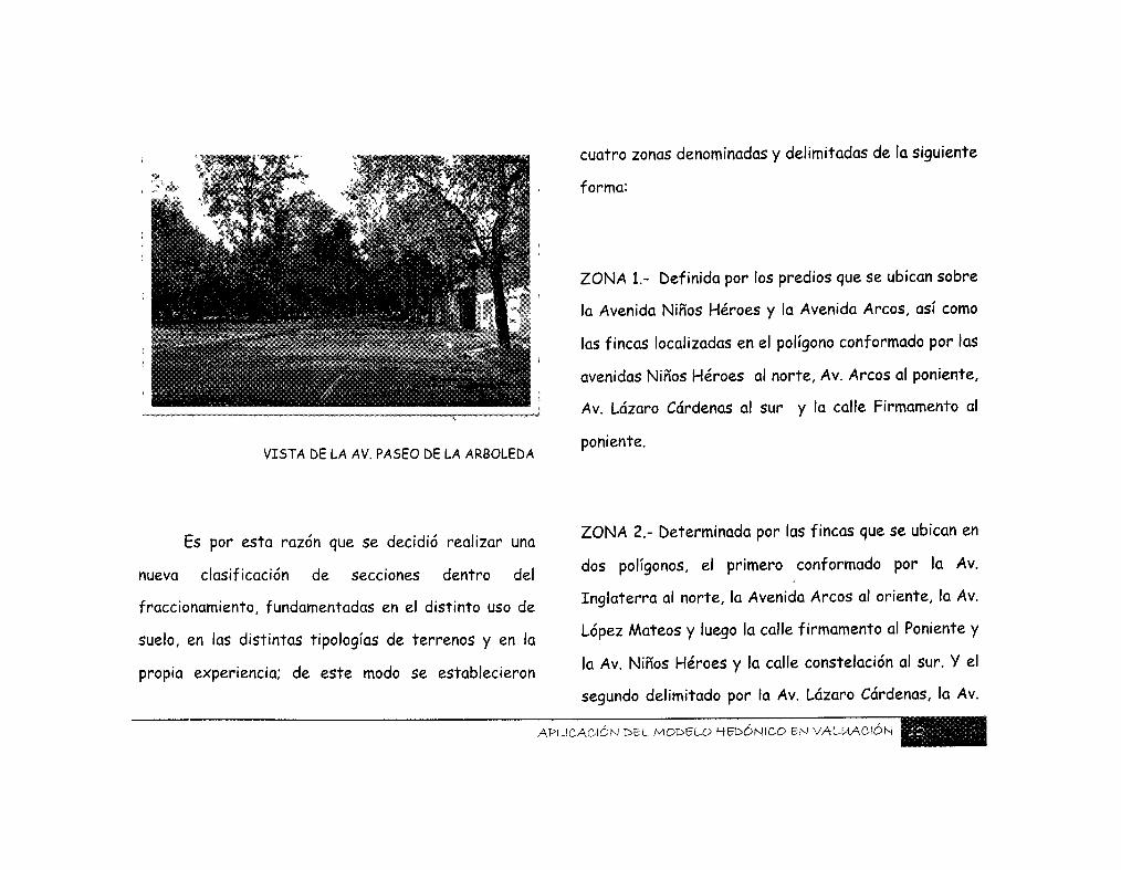
VISTA DE LA AV. PASEO DE LA ARBOLEDA
Es por esta razón que se decidió realizar una
nueva clasificación de secciones dentro del
fraccionamiento, fundamentadas en el distinto uso de
suelo, en las distintas tipologías de terrenos y en la
propia experiencia; de este modo se establecieron
cuatro zonas denominadas y delimitadas de la siguiente
forma:
ZONA 1.- Definida por los predios que se ubican sobre
la Avenida Niños Héroes y la Avenida Arcos, así como
las fincas localizadas en el polígono conformado por las
avenidas Niños Héroes al norte, Av. Arcos al poniente,
Av. Lázaro Cárdenas al sur y la calle Firmamento al
poniente.
ZONA 2.- Determinada por las fincas que se ubican en
dos polígonos, el primero conformado por la Av.
Inglaterra al norte, la Avenida Arcos al oriente, la Av.
López Mateos y luego la calle firmamento al Poniente y
la Av. Niños Héroes y la calle constelación al sur. Y el
segundo delimitado por la Av. Lázaro Cárdenas, la Av.
LIGACIÓN DEL MODELO HEDÓNICO EN VALUACIÓN
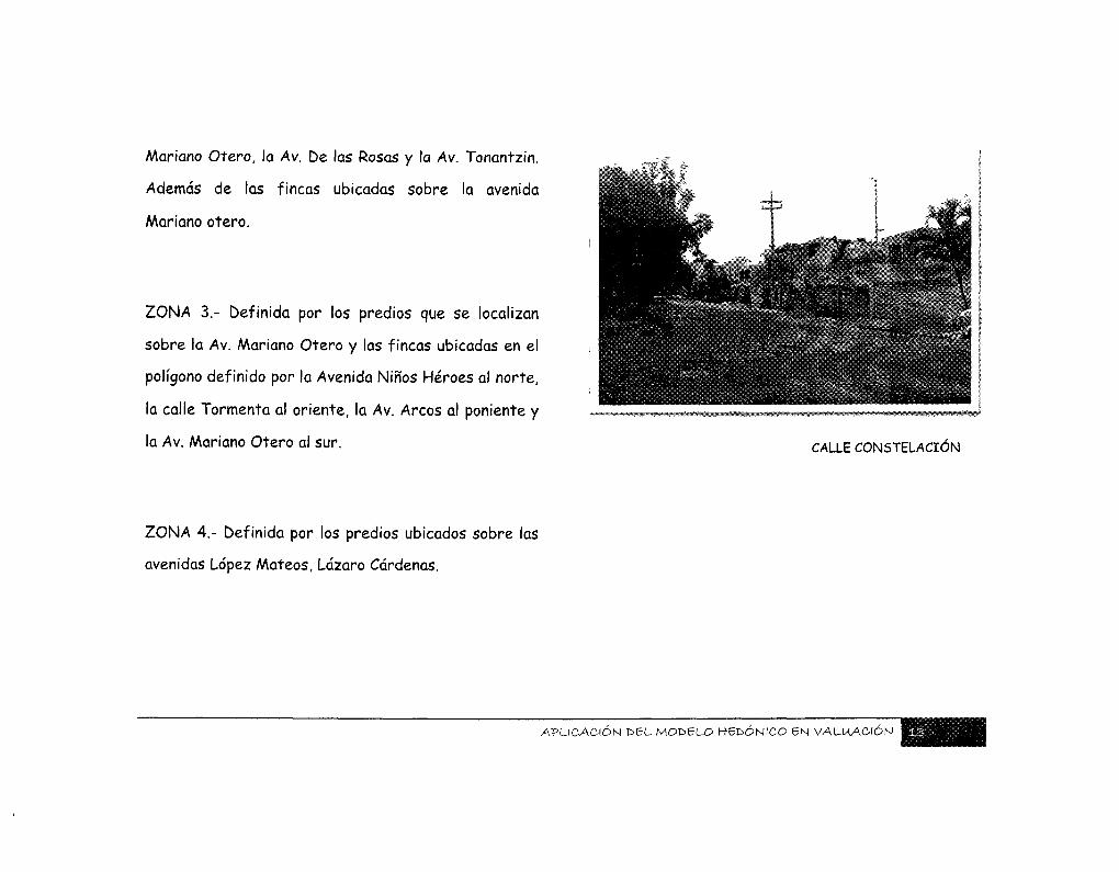
Mariano Otero, la Av. De las Rosas y la Av. Tonantzin.
Además de las fincas ubicadas sobre la avenida
Mariano otero.
ZONA 3.- Definida por los predios que se localizan
sobre la Av. Mariano Otero y las fincas ubicadas en el
polígono definido por la Avenida Niños Héroes al norte,
la calle Tormenta al oriente, la Av. Arcos al poniente y
la Av. Mariano Otero al sur.
ZONA 4.- Definida por los predios ubicados sobre las
avenidas López Mateos, Lázaro Cárdenas.
CALLE CONSTELACIÓN
APLICACIÓN &ELMOt>eLO HecÓNICO BN VALUACIÓN
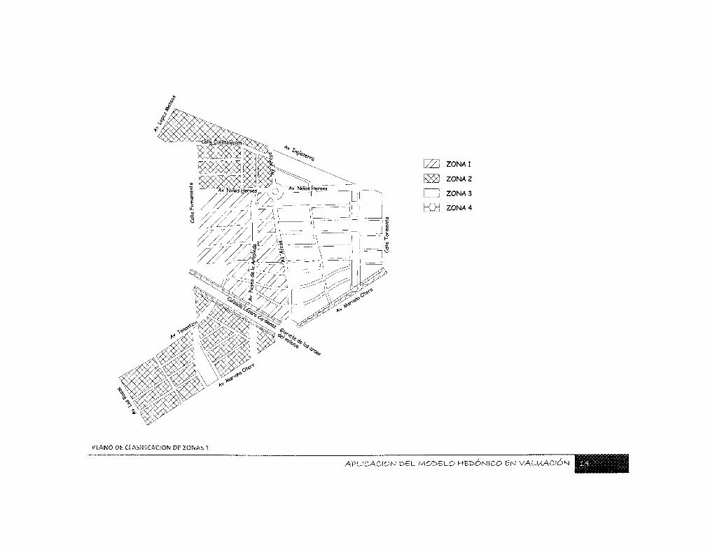
[771 Z0NA1
KSHI ZONA 2
I i ZONA 3
RTj ZONA 4
PLANO Dfc CI AS1FÍCACION DF ZOfMAS 1
A P L I C A C I Ó N D E L M O D E L O H E D O N I C O E N V A L U A C I Ó N feS^aaáL*

I I t . -OFERTA t>B V IVIENDA EN
APLICACIÓN UELMOtsELO H£r>ONICO EN VALUACIÓN

3.±.-T>BFlN\C\ON y
INSCRIPCIÓN t>B L A S
CAT^ACTB-RÁSTl CAS
ANAU2LAV>AS
Esta nueva zonificación se utilizó como uno de
las características observadas dentro de la regresión,
además de las que a continuación se definen.
PRECIO.- Definido como el valor de venta del
inmueble sin considerar descuentos ni negociaciones.
TERRENO.- Cantidad total de metros cuadrados
de terreno que posee el bien.
METROS CUADRADOS DE CONSTRUCCIÓN.-
Considerando todas las áreas techadas de manera
permanente que posea el edificio, incluyendo terrazas,
cuartos de servicio, cochera, etc. Sin importar
clasificaciones ni tipologías.
NÚMERO DE NIVELES.- cuantifica todos los
niveles que posee el inmueble observado.
CACIÓN t>6L MODELO HBHÓNIOO BN VALUACIÓN WM

NÚMERO DE ESPACIOS HABITABLES.- Sala,
comedor, cocina, cocheras techadas, recibidor,
terrazas, recamaras, bibliotecas, cuartos de servicio,
bodegas, etc. Los únicos espacios que en este caso no
son considerados son los baños, ya que estos se
clasifican aparte. En caso de que cualquiera de los
espacios anteriores tenga una superficie mayor a 25
m , como las salas o las terrazas, se podrían considerar
como un espacio mas y se tendría que cuantif icar.
1= predio ubicado en esquina
2=predio no ubicado en esquina
ZONA.- Aquí se asignan el valor de acuerdo a la
ubicación que tenga la finca en relación con el / -
fraccionamiento y que fue descrito en la pagina
anterior.
FRENTE.- La cantidad de metros lineales que
tiene el terreno en su frente a la calle.
NÚMERO DE BAÑOS.- Total de baños que
tenga la propiedad considerando aquellos que solo
tengan lavamanos y w.c. como 0.5 de un baño. EDAD.- Años estimados de vida total que tiene
la casa, sin considerar reparaciones y remodelaciones.
UBICACIÓN CON RESPECTO A MANZANA-
En este caso solo se consideran dos valores:
APLICACIÓN t>BLMOV>£L-0 HBl>ONtCO BN VALUACIÓN
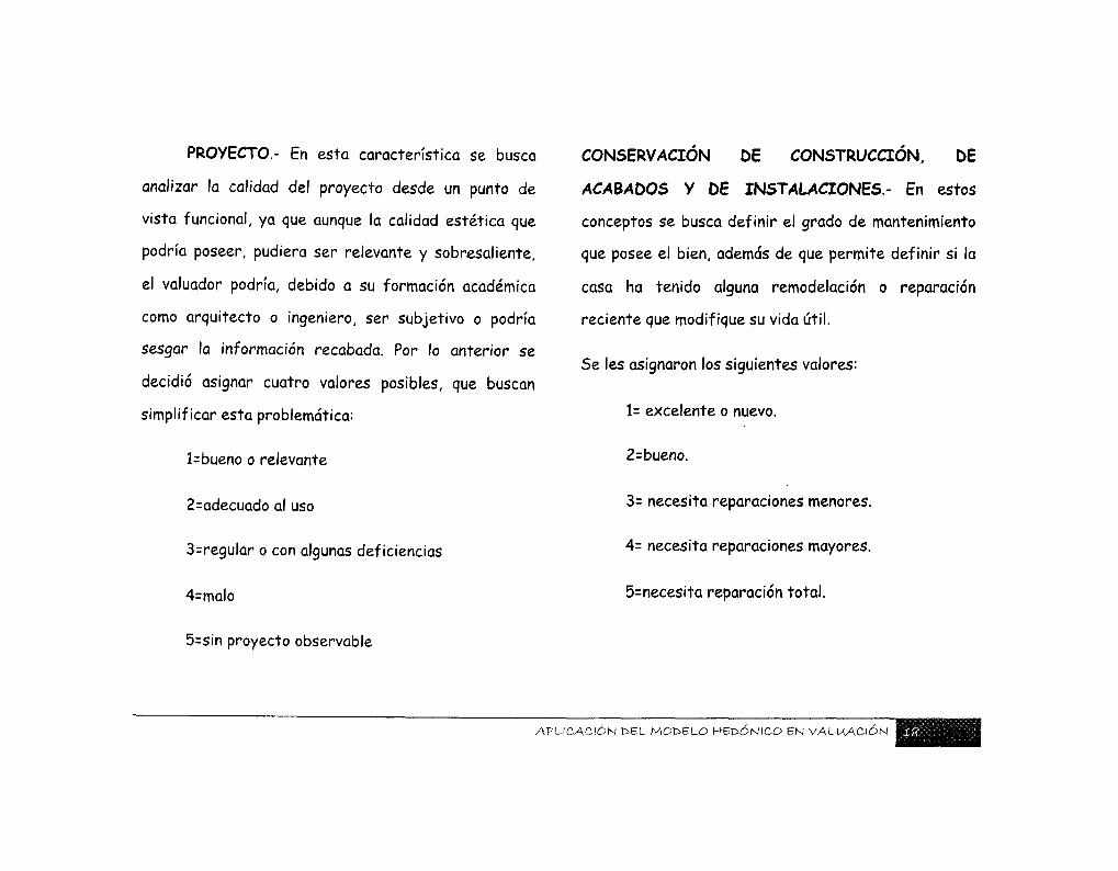
PROYECTO.- En esta característica se busca
analizar la calidad del proyecto desde un punto de
vista funcional, ya que aunque la calidad estética que
podría poseer, pudiera ser relevante y sobresaliente,
el valuador podría, debido a su formación académica
como arquitecto o ingeniero, ser subjetivo o podría
sesgar la información recabada. Por lo anterior se
decidió asignar cuatro valores posibles, que buscan
simplificar esta problemática:
1=bueno o relevante
2=adecuado al uso
3=regular o con algunas deficiencias
4=malo
5=s¡n proyecto observable
CONSERVACIÓN DE CONSTRUCCIÓN. DE
ACABAbOS Y DE INSTALACIONES.- En estos
conceptos se busca definir el grado de mantenimiento
que posee el bien, además de que permite definir si la
casa ha tenido alguna remodelación o reparación
reciente que modifique su vida útil.
Se les asignaron los siguientes valores:
1= excelente o nuevo.
2=bueno.
3= necesita reparaciones menores.
4= necesita reparaciones mayores.
5=necesita reparación total.
CACIÓN t>5L MOISELO HEDÓNICO EN VALUACIÓN
3.2 PRIMER, V>ASO BN LA
APLICACIÓN T>BU M O T I L O
HBV>ÓN\CO
Una vez definidas cuales características son las
que se van a considerar en este estudio y la manera de
cuantificarlas, se procedió a realizar la investigación
de mercado de las fincas en venta en esta zona. El
proceso seguido fue en un primer paso realizar una
llamada telefónica para conocer la información básica,
pero en una segunda etapa fue necesario el realizar
una visita física para poder apreciar correctamente las
características buscadas en este estudio.
Para el proceso de captura se recomienda la
utilización de una hoja de cálculo, para formar una
base de datos que permitan posteriormente
introducirla a algún programa especializado para
calcular la regresión múltiple.
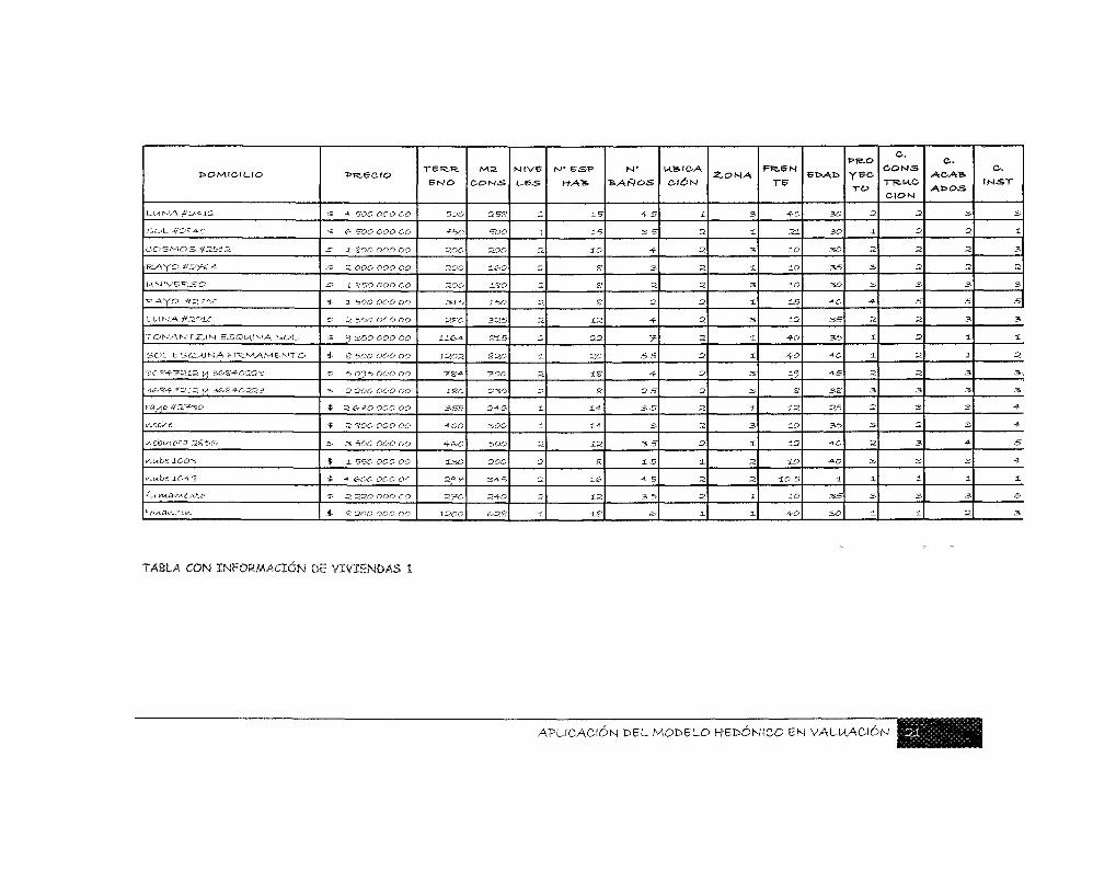
Los datos obtenidos se representan en la
siguiente tabla 1:
LIGACIÓN DELMODELO Het>ONICO BN VALUACIÓN
D O M I C I L I O
L U N A P34-1Z
S O L # 2 f 1 f
C O S M O S -¡É253 2
R Í A y o #2 "^ lT 4
uiMive^-so
P A y O # 2 / ' s í T
L U N A ¡ « 2 5 1 0
T O N A N T i l N E S S W N A S O L -
S O L E S K H I N A F I R M A M E N T O
3 0 « ^ T ^ i a H 3 6 S 4 0 2 3 3
¿ í ^ ? 4 ^ 2 - 1 2 w á ¿ ? 4 0 2 2 3
KCÍL-jD ^ / 2 " ^ 3 0
¡Acoche
í^ebiAiosa zZ5fr
kvwbe 1 0 0 3
i^-ube l o - ? -i
•*L^m.í* flA£l<\.tr
^PlA.atA.^LK.
T»T5.ecio
* 4 5 0 0 O f O OO
* <=- 500 ooo oo
4 x ' í o o í r ^ o o o
4 2; ooo ooo oo
4 -i ? 5 0 o o o o o
^ x <?oo ooo oo
# Z 500 OC O OO
£ 9 3 5 0 o o o oo
* g 5 0 0 OOO OO
4 5 0 5 5 OOO OO
4 a 2 0 0 0 0 0 0 0
* 2 & ^ O OOO OO
$ 3 SOO OOO OO
4 3 5 0 0 0 0 0 00
4 x 5 :5» 0 0 0 00
$ 4 6 0 f ) 0 0 0 c
f 2 2 2 0 0 0 0 co
4 <? 2 0 0 0 0 0 00
6 N O
5 0 0
* 5 0
ZOO
ZOO
zoo
3 1 «>
ZPO
X X & 4
1 2 0 2
T S 4
XJ?O
3 5 5
•f-OO
4 & 0
1 3 0
2^-51
2 5 * 0
X 2 0 0
M 2
O O N S
25??
5 0 0
2 0 0
i & O
xgo
X 5 0
3 2 5
S X 5
S 2 0
TOO
2 3 0
2 4 5
3 0 0
5 D O
2 0 0
34- <5
2 4 0
& 2 2
N i v e L 6 S
2
1
2
2
2
2
2
2
X
2
2
X
1
2
2
2
2
X
H-AÍS.
1 5
X 5
5 0
ff S?
S
X 2
2 2
2 D
X g
s
1 - 4
X 4
X 2
g
i &
1 2
I S
& A Ñ O S
4 5
3 5
4
3
2
2
4
7
5 5
•+ 2 5
3 5
3
3 5
X 5
4 5
3 5
&
M.B-IOA C IÓN
X
2
2
2
2
2
2
2
2
2
2
2
2
2
X
2
2
X
.2,0 NA
3
X
3
X
3
X
3
X
X
3
3
X
3
X
2
2
X
X
F»5.eN -re
4 - 5
2 X
X O
X O
X O
1 5
1 2
-to
+ 0
19
g
X 2
Í O
1 2
X O
XO 5
X O
4 0
S t » A B
3 0
3 0
3 0
3 5
3 0
+ 0
3 5
3 5
+0
• 4 5
3 g
2 5
3 5
+ 0
4 0
1
3 5
S O
P R O
T O
2
X
2
3
3
4
2
1
1
2
3
2
3
2
3
1
3
X
a, O O N S -TR.M.O W O N
2
2
2
2
3
5
2
2
2
2
3
3
2
3
3
X
3
X
O.
A l a o s
3
2
2
2
3
5
3
X
X
3
3
3
3
4
3
X
3
2
I N S T
3
1
3
2
3
5
3
X
2
3 Í
3
4
4
5 '
4
1
5
3
TABLA CON INFORMACIÓN DE VIVIENDAS 1
APLICACIÓN DEL-MODELO HEDÓNICO EN VALUACIÓN
IV . -CÁLCULO T>BU P l^eCIO
tf&frÓ NI CO
T \'¿~~>) T ^.¿-./-f, ¿~~IQ/ -¿—'¡A )
APLICACIÓN t>EL MODELO H-EDONICO 5N VALUACIÓN
4 .1 . - S E ^ K N P O PASO O
CÁUCU.LO r>6L p r e c i o
Una vez obtenida la información anterior el paso
siguiente consiste en aplicar la regresión múltiple, la
cual es un método por medio del cual se relaciona una
variable dependiente que está relacionada con una o
más variables independientes, el objetivo es medir los
cambios que producen las variables independientes (x)
en la variable dependiente (y).
En nuestro caso la variable dependiente es el
precio de venta del inmueble y nuestras variables
independientes son cada una de las características
observadas en los bienes.
La regresión nos arroja, como ya se menciono
anteriormente, los pesos específicos que posee cada
una de las variables independientes más un dato f i jo
que podríamos considerar como una constante; esto se
podría expresar de la siguiente manera-
P(Z)= Zj ai +Z2 a2+ Zn an +C
En donde P(Z) representa el precio hedónico, Zi,
Zn representan cada característica y a„ representan
cada uno de los "pesos específicos" obtenidos en la
regresión para cada una de las características
investigadas y C representa a la constante.
Debemos mencionar que debido a que el objetivo
de esta regresión es la de estimar el valor de nuestra
variable dependiente (precio de venta), entonces
nuestro modelo de estudio será considerado como
modelo con fines predictivos.
^ClÓN DELMODELO HZV>ÓN\CO BN VALUACIÓN E H H f H
Para entender en que consiste nuestro modelo
de regresión, as\ como para interpretar correctamente
los resultados obtenidos, debemos relacionar dos
conceptos; el coeficiente de correlación r, que mide la
relación lineal entre las variables y el análisis de la
varianza. El coeficiente de correlación se eleva al
cuadrado para obtener el coeficiente de determinación
r* y al multiplicarlo por 100 se obtiene el porcentaje
de la varianza de la variable dependiente que queda
explicada por el modelo de regresión.
Al calcular r2 los valores obtenidos deberán
oscilar entre cero y uno, en donde cero significa que
hay poca proporcionalidad entre la variable
dependiente (y) con las variables dependientes (x), y
en caso contrario cuando el valor se acerca a uno, se
considera que existe una gran proporcionalidad entre
las variables.
Este modelo necesita ser validado, para comprobar si es el más adecuado, y para las regresiones lineales se utiliza la técnica denominada como el método de los mínimos cuadrados.
Este método consiste en calcular la suma de las distancias al cuadrado entre los puntos reales y los puntos definidos por la recta estimada a partir de las variables introducidas en el modelo, de forma que la mejor estimación será la que minimice estas distancias.10
Así mismo se obtiene el grado de
"significatividad de F" o también conocido como "P
value", el cual deberá ser menor que .05 para
considerar que hay correlación entre las variables.
Una vez revisado todo el modelo y habiendo
checado que tanto los valores de r2 como el de
significatividad de F estén dentro de los parámetros,
debemos revisar que también cada una de las
(PELAEZ, 2006)
6 N DEL MODELO H-EDÓNICO EN VALUACIÓN
características observadas sea significativa para el
modelo, por lo tanto se necesita observar que cumplan
con el parámetro de la signif icatividad de f.
De no ser así, entonces es necesario realizar una
revisión del modelo hasta encontrar cuales de las
características observadas poseen una mayor
correlación.
Dado que el objetivo de esta tesis es la de
implementar un mecanismo de fácil aplicación para un
arquitecto o ingeniero que se dedique a la valuación, se
decidió no desarrollar toda esta regresión, ni la
revisión de el modelo de forma manual, si no a través
de la utilización de un programa especializado en
estadística, pero de fácil manejo como es el caso del el
programa "Statgraphics" de la compañía "Statical
Graphics Corp", de tal modo a continuación se presenta
el análisis de nuestro modelo propuesto.
Como nota adicional se debe mencionar que en un
principio se busco utilizar un programa de hoja de
cálculo para realizar la regresión, pero al no ser un
programa especializado no fue practico ya que no se
pudo realizar la revisión completa del modelo.
Aún asi en la sección de anexos se encuentra el
proceso para implementarlo en el programa Excel de
Microsoft.
-ICACIÓN DEL MODELO HEDÓNICO EN VALUACIÓN
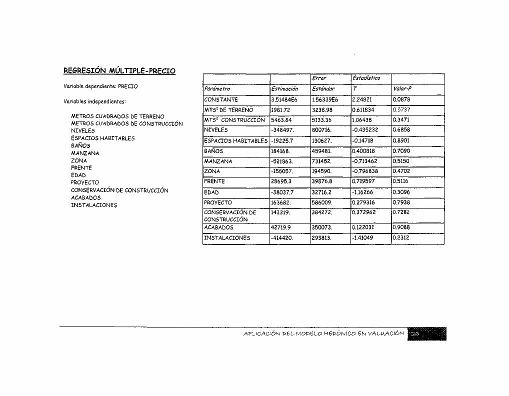
REGRESIÓN MÚLTIPLE-PRECIO
Variable dependiente: PRECIO
Variables independientes:
METROS CUADRADOS DE TERRENO METROS CUADRADOS DE CONSTRUCCIÓN NIVELES ESPACIOS HABITABLES BAÑOS MANZANA ZONA FRENTE EDAD PROYECTO CONSERVACIÓN DE CONSTRUCCIÓN ACABADOS INSTALACIONES
Parámetro
CONSTANTE
MTS2 DE TERRENO
MTS2 CONSTRUCCIÓN
NIVELES
ESPACIOS HABITABLES
BAÑOS
MANZANA
ZONA
FRENTE
EDAD
PROYECTO
CONSERVACIÓN DE CONSTRUCCIÓN
ACABADOS
INSTALACIONES
Estimación
3.51484E6
1981.72
5463.84
-348497.
-19225.7
184168.
-521863.
-155057.
28695.3
-38037.7
163682.
143319.
42719.9
-414420.
Error
Estándar
1.56339E6
3238.98
5133.36
800716.
130627.
459481.
731452.
194590.
39876.8
32716.2
586009.
384272.
350073.
293813.
Estadístico
T
2.24821
0.611834
1.06438
-0.435232
-0.14718
0.400818
-0.713462
-0.796838
0.719597
-1.16266
0.279316
0.372962
0.122031
-1.41049
Valor-P
0.0878
0.5737
0.3471
0.6858
0.8901
0.7090
0.5150
0.4702
0.5116
0.3096
0.7938
0.7281
0.9088
0.2312
APLICACIÓN E>6L MODELO HEDONICO 6N VALUACIÓN
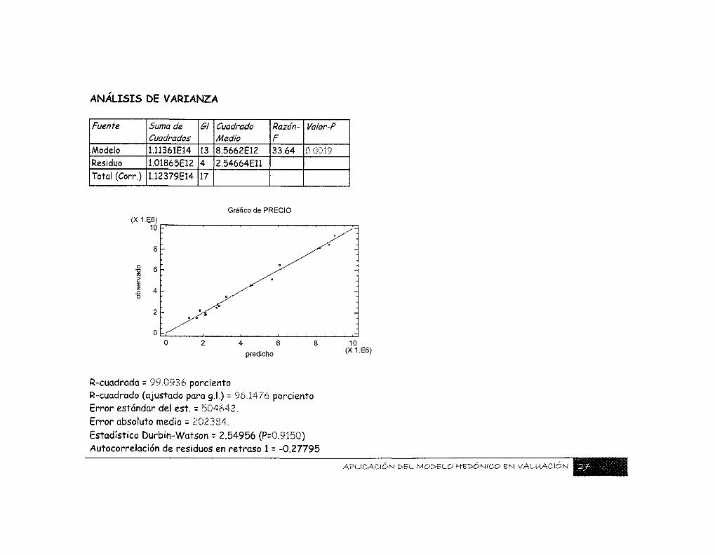
ANÁLISIS DE VARIANZA
Fuente
Modelo Residuo Total (Corr.)
Suma de Cuadrados 1.11361E14
1.01865E12 1.12379E14
61
13 4 17
Cuadrado Medio 8.5662E12 2.54664E11
Razón-F 33.64
Valor-P
0,0019
Gráfico de PRECIO (X1.E6)
10 F
<¡> w
JO O
predicho 10
(X1.E6)
R-cuadrada = 99.0936 porciento R-cuadrado (ajustado para g.l.) = 96.1476 porciento Error estándar del est. = 504642. Error absoluto medio = 202384. Estadístico Durbin-Watson = 2.54956 (P=0.9150) Autocorrelación de residuos en retraso 1 = -0.27795
APLICACIÓN t>EL MODELO Het>ONICO EN VALUACIÓN
De acuerdo a los datos anteriores observamos lo siguiente:
1) La r2 del modelo explica el 99.0936% de la variabilidad en PRECIO (variable dependiente)
2) Puesto que el valor de significatividad encontrado de .0019 cumple con ser menor a .005 existe una relación significativa entre las variables con un nivel de confianza del 95%.
3) Que ninguna de nuestras variables dependientes fueron estadísticamente significativas en lo individual ya que ninguna cumple con el modelo, ya que su valor de significatividad o de p-value es mayor a .005.
Debido a lo anterior es necesario re-calcular nuestro modelo ya que de acuerdo al proceso seguido en toda regresión debemos encontrar el modelo más significativo estadísticamente.
APLICACIÓN MLMODELO HBV>ÓN\CO EN VALUACIÓN V • ^ . " f f i i *
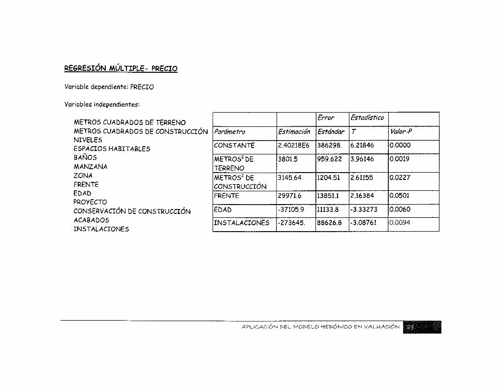
REGRESIÓN MÚLTIPLE- PRECIO
Variable dependiente: PRECIO
Variables independientes:
METROS CUADRADOS DE TERRENO
METROS CUADRADOS DE CONSTRUCCIÓN NIVELES ESPACIOS HABITABLES BAÑOS MANZANA ZONA FRENTE EDAD PROYECTO CONSERVACIÓN DE CONSTRUCCIÓN ACABADOS INSTALACIONES
Parámetro
CONSTANTE
METROS2 DE TERRENO METROS2 DE CONSTRUCCIÓN FRENTE
EDAD
INSTALACIONES
Estimación
2.40218E6
3801.5
3145.64
29971.6
-37105.9
-273645.
Error
Estándar
386298.
959.622
1204.51
13851.1
11133.8
88626.8
Estadístico
T
6.21846
3.96146
2.61155
2.16384
-3.33273
-3.08761
Valor-P
0.0000
0.0019
0.0227
0.0501
0.0060
0.0094
APLICACIÓN DEL MODELO H+EDONICO EN VALUACIÓN
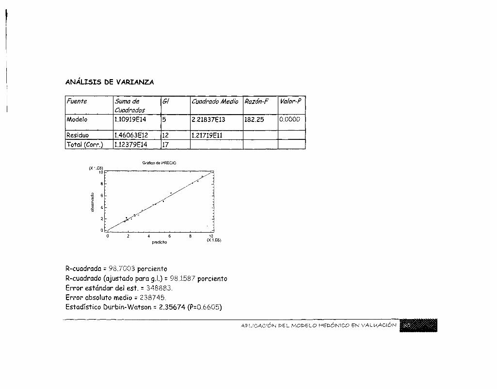
ANÁLISIS DE VARIANZA
Fuente
Modelo
Residuo Total (Corr.)
Suma de Cuadrados 1.10919E14
1.46063E12 1.12379E14
Gl
5
12 17
Cuadrado Medio
2.21837E13
1.21719E11
Razón-F
182.25
Valor-P
0,0000
Gráfico de PRECIO (X1.E6)
1 n ,-r- — , , , . , -
predicho < X 1 E 6 )
R-cuadrada = 98.7003 porciento R-cuadrado (ajustado para g.l.) = 98.1587 porciento Error estándar del est. = 348883. Error absoluto medio = 238745, Estadístico Durbin-Watson = 2.35674 (P=0.6605)
APLICACIÓN E>EL hAOT>BLO HBX^ÓNICO EN VALUACIÓN ¡111
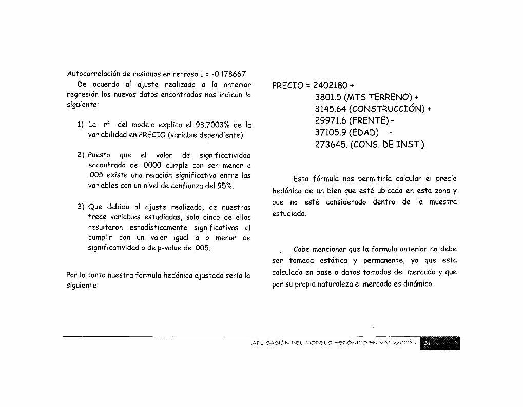
Autocorrelación de residuos en retraso 1 = -0.178667 De acuerdo al ajuste realizado a la anterior
regresión los nuevos datos encontrados nos indican lo siguiente:
1) La r2 del modelo explica el 98.7003% de la variabilidad en PRECIO (variable dependiente)
2) Puesto que el valor de significatividad encontrado de .0000 cumple con ser menor a .005 existe una relación significativa entre las variables con un nivel de confianza del 95%.
3) Que debido al ajuste realizado, de nuestras trece variables estudiadas, solo cinco de ellas resultaron estadísticamente significativas al cumplir con un valor igual a o menor de significatividad o de p-value de .005.
Por lo tanto nuestra formula hedónica ajustada sería la siguiente:
PRECIO = 2402180 + 3801.5 (MTS TERRENO) + 3145.64 (CONSTRUCCIÓN) + 29971.6 (FRENTE) -37105.9 (EDAD) -273645. (CONS. DE INST.)
Esta fórmula nos permitiría calcular el precio
hedónico de un bien que esté ubicado en esta zona y
que no esté considerado dentro de la muestra
estudiada.
Cabe mencionar que la formula anterior no debe
ser tomada estática y permanente, ya que esta
calculada en base a datos tomados del mercado y que
por su propia naturaleza el mercado es dinámico.
9N t>ei_ MOt>5LO H e t Ó N I C O EN VALUACIÓN
En el caso específico de la zona de estudio de
esta tesis se podría considerar que debido al estado
de nuestra economía y a que no se proyectan acciones
urbanísticas que modifiquen significativamente la
traza urbana de esta colonia ni a su percepción
comercial, la vigencia de nuestra base de datos seria
de un año.
APLICACIÓN V>BL MODELO HEDÓNICO SN VALUACIÓN
/ /
V.- REALIZACIÓN Ü6 A V A L A O S
COMERCIA LES
APLICACIÓN DEL MODELO H+EDONICO BN VALUACIÓN

Para tratar de mantener un enfoque objetivo en
esta tesis, se determinó que los avalúos que se
utilizarían para comprobar el modelo antes descrito,
deberían de ser realizados por un valuador
independiente.
Por esta razón se le solicito al Arq. Juan Manuel
Bravo Armejo que nos facilitara algunos avalúos que él
hubiera realizado en esta zona en un tiempo reciente.
Cabe mencionar que por solicitud del arquitecto,
algunos datos fueron omitidos por privacidad de la
información de sus clientes, de manera que a
continuación se presentan los extractos de los mismos
con la información más relevante.
Debemos aclarar que algunos de estos avalúos
fueron realizados en el 2007, pero se considero
utilizarlos manifestando previamente esta
condicionante.
Además se debe aclarar que la opinión de valor
manifestada en estos avalúos puede variar de la
obtenida a través del modelo hedónico, debido
principalmente a los métodos seguidos para obtener
ese valor.
Ya que mientras el modelo hedónico manifiesta
el valor de mercado "puro" en base a determinadas
características observadas; los modelos tradicionales
de valuación dependen en un gran porcentaje de la
experiencia y capacidad del propio valuador, y de la
aplicación de distintas metodologías sujetas a
interpretaciones y por lo tanto no objetivas en un
término amplio.
ÓN DEL. MOE>eL0 HBt>ÓNICO EN VALUACIÓN
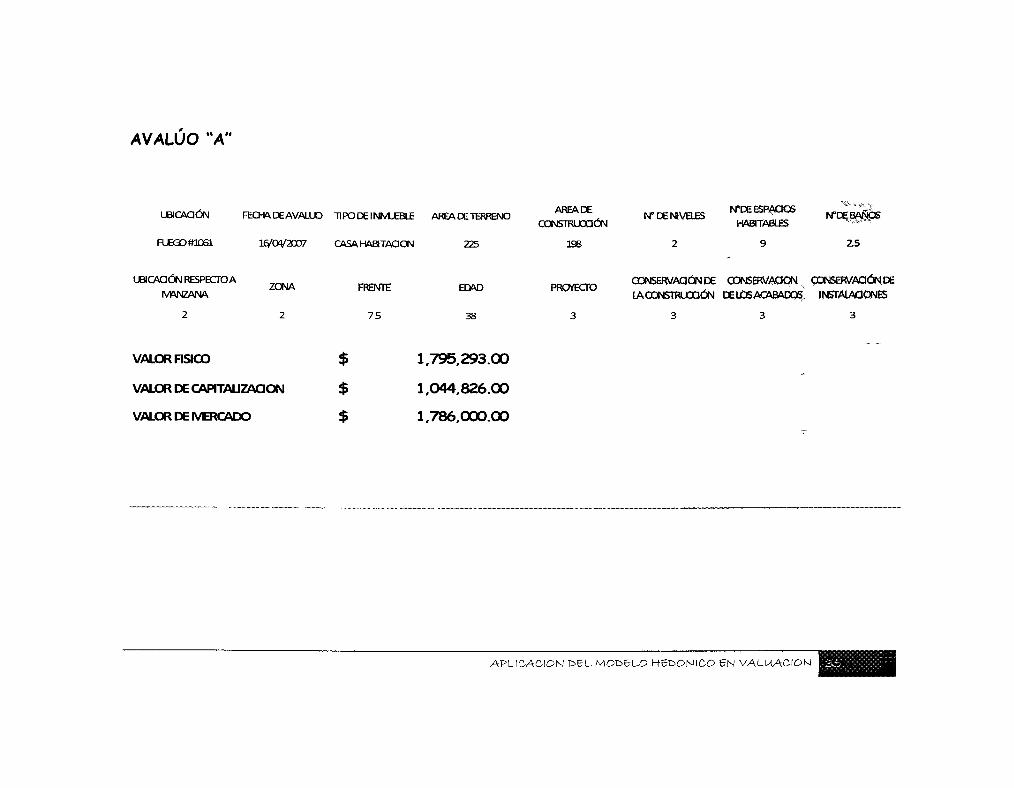
AVALÚO "A"
UHCACJÓN
FUEGO #1061
UBICACIÓN RESPECTOA
MANZANA
FECHA DE AVALUÓ TIFO DE INMUEBLE AREA DETERRENO
l#Oy20O7 CASAHABITAaON 225
ZONA
VALOR FÍSICO $
VALOR DE CAPITALIZACIÓN $
VALOR DE IVERCADO $
FRENTE
7 5
EDAD
38
1.795,293.00
1,044,826.00
1,786,000.00
AREA DE
CONSTRUCaÓN
198
PROYECTO
N" DE NIVELES
2
N"DE ESPACIOS HABITABLES
Z5
CONSERVAaÓNDE CONSERVACIÓN N CONSEWAGtáNDE
LACONSTRUXJON D£10SACAB(VD0¿ INSTALAaONES
APLICACIÓN DEL MODELO H5E>ONICO EN VALUACIÓN

AVALUÓ "B'
NOCHE #2442
UBICACIÓN RESPECTOA
ÍVANZANA
FECHADEAVAUÚO TIPODEINMJEBIE AREA DETERRENO
16/04/2007 CASAI-WBITAaÓN 680
ZONA
VALOR FISCO
VALOR DE CAPITALIZACIÓN
VALOR DE MERCADO
$
$
FRENTE
25
EDAD
32
5,886,540.00
S I N DATO
5,903,000.00
AREA DE
CONSTRUXIÓN
743.5
PROYECTO
N°JDE NIVELES
3
N T E ESPACIOS
HABITAJ3LES
26
N"DEBAÑ0Sx
5.5
CONSERVACIÓN DE CONSERVAaON CONSERVACIÓN DE
LACONSTRUaaÓN DEIOSACABADOS U^TAtApQNES
APLICACIÓN DEL MODELO KEÜONICO EN VALUACIÓN

AVALÚO "C
IBICACIÓN FECHA DE AVALÚO 71PODEINMJEBIE AREA DETERRENO
NEBUOSA#2856 16/04/2007 CASA HABITAQÓN 600
AREA DE
CONSTRUCTION
470
N* DE NIVELES N°D£ ESPACIOS
- HABITABLES-
18
WDE BAÑOS
ilk*
55
UBICACIÓN RESPECTDA
IVANZANA ZONA
VALOR FÍSICO
VALOR DE CAPITALIZACIÓN
VALOR DE IVERCADO
$
$
$
FRENTE
15
EDAD
35
3,909.301.00
2,199.043.00
3.299,000.00
PROYECTO CONSERVAPÓNDE , GONSJRVAOON , CONSERVAaÓfel DE
LACONSTRUGCtÓN DE LOS ACABADOS^ INSTALACIÓN©^
A P L I C A C I Ó N E>6L M O C Ó L O H E D O N I C O E N V A L U A C I Ó N
COMPARACIÓN T>£ R .5S(ALTADOS
APLICACIÓN D E L M O D 5 L O HBV.ÓNIOO EN VALUACIÓN
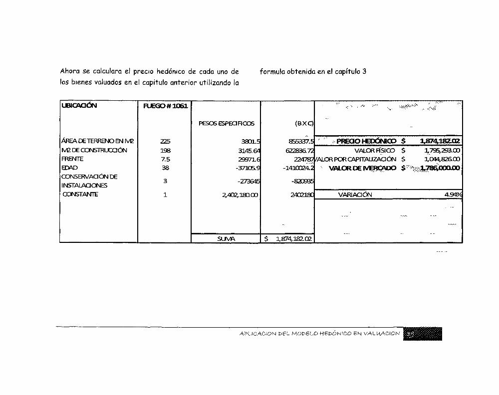
Ahora se calculara el precio hedónico de cada uno de
los bienes valuados en el capitulo anterior utilizando la
formula obtenida en el capítulo 3
UBICACIÓN
ÁREA DE "TERRENO EN M2
IVE DE CONSTRUCCIÓN
FRENTE
EDAD
CONSERVACIÓN DE
INSTALAaONES
CONSTANTE
FUEGO # 1 0 6 1
225
198
7.5
38
3
1
PESOS ESPEa FIGOS
3801.5
3145.64 299716
-37105.9
-273645
2,402,180.00
SUVA
( B X Q
855337.5
62283672 224787
-1430024.2
-820935
240218C
$ 0,874,182.02
PREOO HEDÓNICO $ 1,874,182.02
VALOR FÍSICO $ :U795,293.00
/ALORPORCAPITAUZAOÓN $ 3,044,82600
*- VALOR DE IVERCADO $ ^ í j & 7 S & 0 0 a 0 a
VAFüAaÓN 4.949Í
—
APLICACIÓN E>gL MODELO HBV>ON\CO BN VALUACIÓN
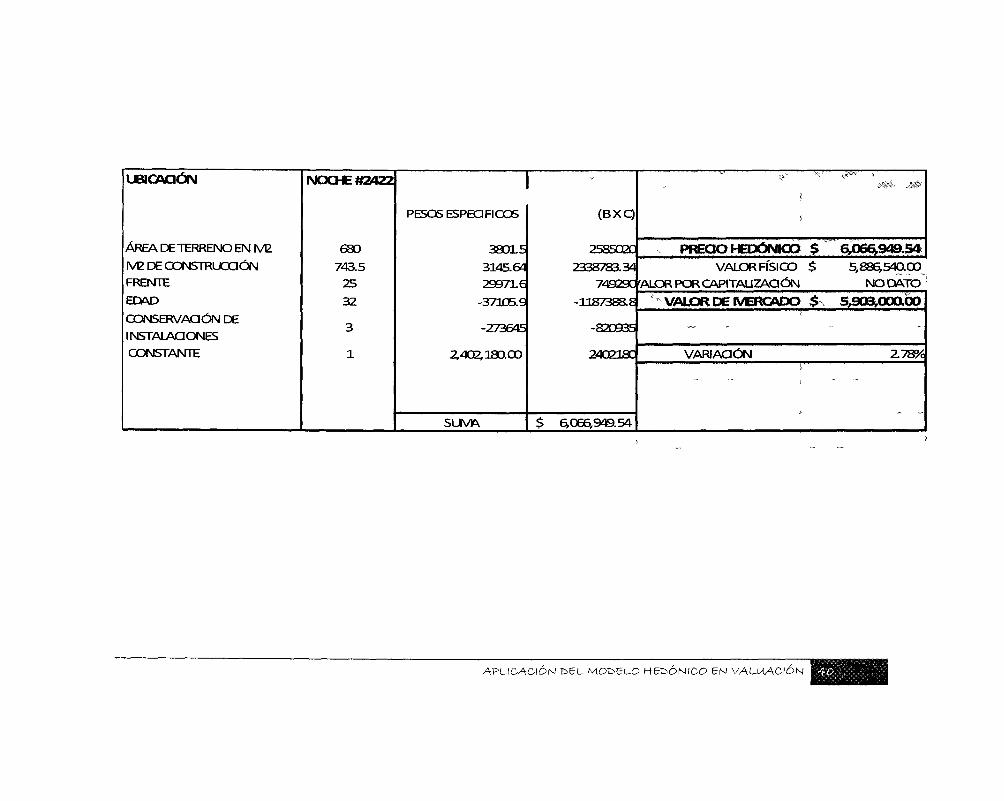
UBICACIÓN
ÁREA DE TERRENO EN M2
M2 DE ODNSmUGaÓN FRENTE
EDAD
CONSERVACIÓN DE
INSTALACIONES CONSTANTE
NOCHE #2422
680
743.5 25
32
3
1
PESOS ESPEO FIGOS
38015
3145.64 299716
-37105.9
-273645
2,402,180.00
SUVA
( B X Q
258502C
2338783.34 74929C
-U87388.8
-820935
24021SC
$ 6,066,949.54
I
í
PRECIO HEDÓNICO $
VALOR FÍSICO $ 'ALOR POR CAPITAUZAOÓN
VALOR DE IVERCADO $
VARIAOÓN
4W ' a '
6,066,949.54
5,886,54Q00 NO DATO
5,903,000.C»
Z789Í
. .
APLICACIÓN DEL MODELO KEDONICO EN VALUACIÓN
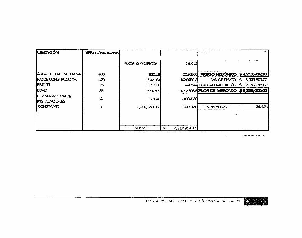
UBICACIÓN
ÁREA DE TERRENO EN M2
M2 DE CONSTRUGa ÓN
FRENTE
EDAD
CONSERVACIÓN DE INSTALACIONES CONSTANTE
NEBULOSA #2856
600
470 35
35
4
1
PESOS ESPEO FIGOS
38015
3145.64 299716
-37105.S
-273645
2,402,180.00
SUVA
1 ( B X Q
2280900
1478450.8
449574
-1298706.5
-1094580
24021BC
$ 4,217,818.30
w *# v \ ^
PRCaOHEDÓNICO $4 ,217,81R30
VALOR FÍSICO $ 3,909,30100
PORCAPITAUZAOÓN $ 2,159,043.00
ALOR DE MERCADO $3,259,00a0O
VARIAOÓN 29.42%
*
APLICACIÓN t>EL MODELO HEDÓNICO EN VALUACIÓN E
Al analizar los anteriores ejemplos podemos
obtener las siguientes conclusiones:
a) Como el mismo Rosen sostiene en su teoría de la
igualación de las diferencias11, es necesario que
al comparar distintos elementos encontremos
las diferencias que nos permitan diferenciar las
similitudes.
b) En el tercer caso la diferencia entre el valor
hedónico con el obtenido a través del avalúo es
de un 29.4% lo cual es significativo y nos
permite aventurar al afirmar que esta
diferencia tan marcada está relacionada con los
comparables y con los factores utilizados en la
homologación, ya que al observar el avalúo
encontramos que se manejaron factores iguales
para fincas ubicadas en zonas diferentes dentro
de la misma colonia.
(Cartwright, 2001)
c) En los dos primeros casos la diferencia fue
mínima ya que fue menor al 5%, aunque como se
menciono anteriormente, los valores del avalúo
fueron obtenidos en el 2007 y se tendría que
ajusfar la depreciación y comprobar los
comparables, aunque en este sentido podemos
afirmar que el mercado de viviendas en esta
zona ha mantenido desde el año anterior una
tendencia uniforme en el valor de sus fincas.
N t>ELMOE>EUO KeDÓNICO EN VALUACIÓN ¡ é M M t & ü f e
Vil .- CONCLUSIONES y
^ C O M E N T A C I O N E S
APLICACIÓN DEL MODELO HEDÓNICO EN VALUACIÓN
El modelo de los precios hedónicos es un método
que logra explicar de una manera más completa cuales
son las condiciones de mercado de determinado
producto, pudiendo incluso aplicarse tanto a la
vivienda, como en el caso de esta tesis, como a
productos tan distintos y diferentes como los autos,
las computadoras, y cualquier producto en general que
despierte un interés en poseerlo.
Este modelo apenas comienza a aplicarse en
nuestro país, aunque ya se hace con bastante
regularidad en algunos de Europa, asi como en países
de centro y sud-América, por lo tanto será normal que
cause confusión y desconfianza provocadas por el
desconocimiento del mismo.
La tarea de todo profesional es la constante
actualización de su conocimiento que le permita
desarrollar su trabajo de una manera más eficaz y
satisfactoria para él y para sus clientes, por lo tanto
es necesario mantener una actitud abierta ante nuevo
conocimiento, aunque este ponga en entredicho algunos
de los conceptos aprendidos con anterioridad.
Aplicaciones y modelos como el que se describe
en este trabajo se convierten en útiles herramientas
para el valuador, as\ como parámetros dentro de los
cuales pueda ubicar y comparar los valores obtenidos a
través de otras metodologías.
Además de lo anterior, es necesario mencionar
que uno de los objetivos de este trabajo fue, el
presentar la información de una manera lo más clara y
sencilla posible, para sea comprensible para cualquier
profesional de la valuación que le interese ampliar su
conocimiento.
¿>N t>EL MODELO HECÓNICO BN VALUACIÓN MEE

El método hedónico plantea algunas
problemáticas para ¡mplementarlo y estas tienen que
ver con la información, la cual es la principal
problemática de cualquier actividad intelectual del
hombre; ya que para poder calcular y encontrar las
coincidencias donde se encuentran las distintas
características que poseen los bienes, es necesario que
nuestra información sea lo más pura, objetiva y clara
posible.
Por esta razón en esta tesis se busco que las
características analizadas de los bienes fueran fáciles
de determinar a\ realizar una inspección de cualquier
finca, ya que aunque partían de una apreciación
subjetiva de este investigador al postularlas, se
buscaba que no estuvieran sujetas a una interpretación
subjetiva al momento de observarlas; lo cual
contaminaría la información.
Además de que si nuestra base de datos
contenía información verídica y clara, entonces
permitiría la aplicación correcta de este modelo.
Debemos mencionar también que a pesar de que
en un principio se consideraron trece características,
que según nuestro criterio, afectaban el valor de los
bienes; una vez ajustada la regresión de acuerdo a su
propia metodología, encontramos que no todas eran
estadísticamente relevantes.
Esto en un principio podría pensarse que
contradice el postulado principal de la teoría de los
precios hedónicos, pero es todo lo contrario, ya que al
aplicar esta metodología se elimina lo subjetivo de la
determinación de las características a analizar ya que
la regresión arroja solo las que son estadísticamente
relevantes al modelo en lo general.
De esta manera permite que el valuador obtenga
una herramienta sustentada, matemática y objetiva,
¿N DEL MOCÓLO HBVÓNICO EN VALUACIÓN te^MI^M
que le permita obtener un parámetro para comparar el
valor obtenido contra el calculado a través de los
métodos tradicionales de valuación; los cuales en la
mayoría de los casos están impregnados de una gran
subjetividad, tanto en el método como en el factor
humano que los calcula.
APLICACIÓN t>BL MODELO HB&ÓNICO EN VALUACIÓN 1 1

VIII.- B IBLIOGRAFÍA
APLICACIÓN DEL MODELO HEDONICO BN VALUACIÓN
"A Spatial Equilibrium Model of the Livestock-Feed Economy in the United States" [Publicación periódica] / aut. Fox K. A.. - [s.l.]:
Econometrica, 1953.
"JARDINES DEL BOSQUE" BARRAGAN Y EL HABITAT 1955-2005
[Conferencia] / aut. GOMEZ SUSTAITA GUILLERMO, TOMAS DE
HIJAR ÓRNELAS, ILDEFONSO LOZA MÁRQUEZ. - GUADALAJARA,
JALISCO : H. AYUNTAMIENTO DE GUADALAJARA, 2005.
"MODELOS DE REGRESIÓN: LINEAL SIMPLE Y REGRESIÓN
LOGÍSTICA" [En línea] / aut. PELAEZ IRENE MORAL//
http://www.seden.org/files/14-CAP%2014.pdf. - 2006.
"On the theory of equalizing differences; Increasing abundances of
types of workers may increase their earnings" [Publicación
periódica] / aut. Cartwright Edward and Myrna Wooders / /
Economics Bulletin, Vol 4, N°4 pp. 1-10. - 2001.
"Price Indexes and Quality Change. Stuides in New Methods of
Measurement [Publicación periódica] / aut. Griliches Zvi. -
Cambridge Massachusetts: Harvard University Press,, 1971.
ESTADÍSITCA Y ECONOMETRÍA [Libro] / aut. DOMINICK SALVATORE
DERRICK REAGLE. - MADRID : MCGRAW-HILL/ INTERAMERICANA DE
ESPAÑA, S.A.U, 2004.
GACETA MUNICIPAL [Libro] / aut. GUADALAJARA AYUNTAMIENTO
DE. - GUADALAJARA : AYUNTAMIENTO DE GUADALAJARA, 2004. -
Vol. ADF.
HEDONIC PRICES AN IMPLICIT MARKETS: PRODUCT
DIFFERENTIATION IN PURE COMPETITION [Publicación periódica] /
aut. SHERWIN ROSEN. - CHICAGO : THE JOURNAL OF POLITICAL
ECONOMY, 1974. - Vol. 82.
HEDONIC PRICES AND IMPLICIT MARKETS: PRODUCT
DIFFERENTIATION IN PURE COMPETITION [Publicación periódica] /
aut. ROSEN SHERWIN. - CHICAGO : THE JOURNAL OF POLITICAL
ECONOMY, 1974. - Vol. 82 N" 1.
INTRODUCCIÓN A LA ECNOMETRÍA [Libro] / aut. FRANCISCO TRÍVEZ
BIELSA. - MADRID : EDICIONES PIRÁMIDE, 2004.
INTRODUCCIÓN A LA ECONOMETRÍA [Libro] / aut. PETER
KENNEDY. - MÉXICO, D.F.: FONDO DE CULTURA ECONÓMICA, 1997.
SHERWIN ROSEN, BIOGRAFICAL MEMOIR [Publicación periódica] /
aut. LAZEAR EDWARD P.. - Washington, D.C : The National
Academic Press, 2003. - Vol. 83.
6 N V>BL- MODELO H-ECÓNICO EN VALUACIÓN «¿¿y
\X.- ANBXOS
APLICACIÓN DELMOt -ELO H€V>ÓN\CD 5N VALUACIÓN
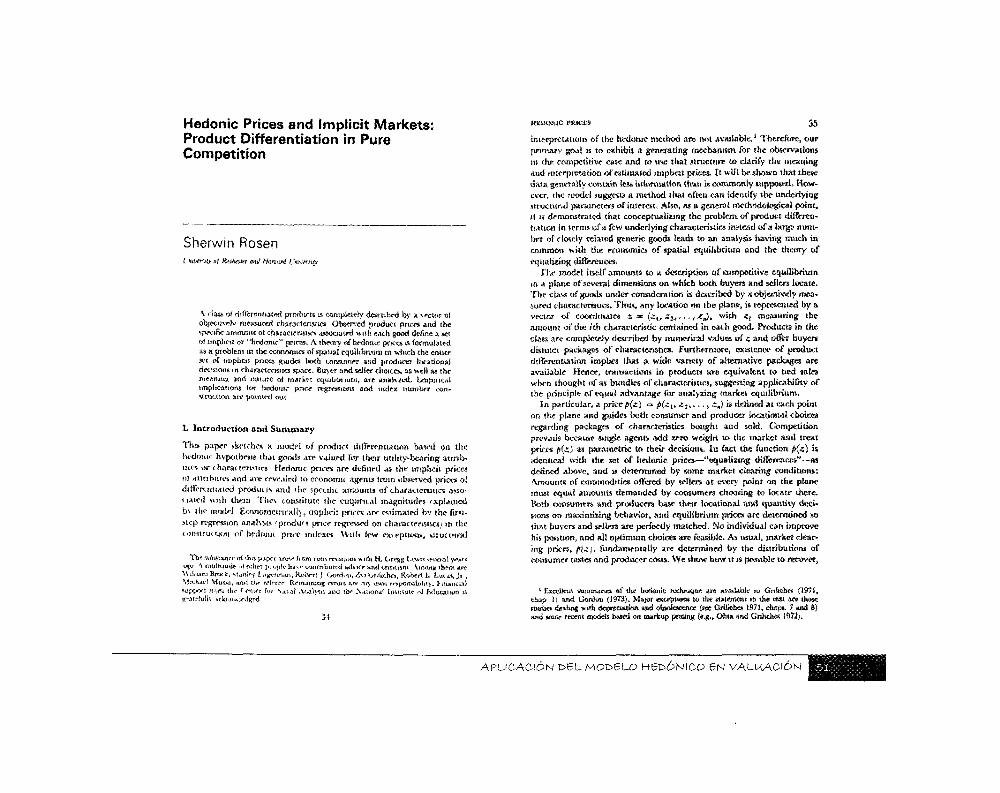
A continuación se presentan, algunos documentos que se consideran importantes como complemento de esta tesis, en primer lugar se agrega el documento original en donde Sherwin Rosen plantea el modelo de los precios hedónicos.
Este documento no es fácil poder encontrarlo ya que fue publicado a manera de artículo, por lo que me permito compartirlo habiendo pagado los derechos correspondientes a la página de internet donde pude localizarlo.
Después de este artículo se presenta una guía para poder implementar la regresión múltiple eñ el programa Excel de Microsoft, para aquellas personas que prefieran utilizar este programa, la guía termina hasta el punto donde se calcula la primera regresión, aunque no se explica la manera de ajustar este modelo para encontrar el que mejor explique la regresión de manera estadística.
APLICACIÓN t>EL MODELO HEDÓNICO EN VALUACIÓN ¡ H i
Hedonic Prices and Implicit Markets: Product Differentiation in Pure Competition
Sherwin Rosen t wwiti s-'f Hteteit** mil Hmwd I'msmty
\ class oí dílteremuíed produrts is completely described by a sector oí obfecitvclv measured rharaeieratics Observed product prices and the specific amounts of charactensifcs associated with each good define a set oi implicit or "hedonir*1 prices. A theory of hedome prices is formulated as a problem in she economics of spatial equilibrium m which the enure set of implicit pnces stades txith consumer ana producer locations! decisions m characteristics space. Buyer ami seller choices, ais well as the meittumi and nature oí market equilibrium, are analvüctt. Lmoiticaí implications tor hedonic pnce regressions and index number construction are pointed out
I. Introduction and Summary
This paper sketches a model of product differentiation bated on the hedonic hypothesis that goods are valued for their utility-bearing aunb» utes oe i ttarai (crones Hedonic pnces arc defined AS the implicit prices oi attributes and are revealed to economic agents irora observed prices oí differentiated produce ¡«id the specific amounts oi" characteristics asso-< lilted Huh ihern Tliev constitute the empirical magnitudes rxplamed b\ the model EconometnraHy, implicit pnces are estimated bv the lim-sicp regression analysis ! produt t price regressed on characteristics; lis the «(instruction of bedotiK price indexes With lew exiepitom, stiuitttral
Tb? subclause oí íhts nappi-aru^ fmm iomcnatiiitrnwith H, {.«relíg l-e1*** *ev£raí y*Mfs I M \ riiuitfiUiip oí elhei juitpii- Iwve (xinfniiut d «duo and criticism \m<mii them arc Hilli-oii BriKk, Stanley tngrmUn.Roltm j Gorclim, ¿'A Ijcitsches, Robert h Lu<,lS,Jt , Mi«K,icl Mys*&, and th<- fri<-r<f Renaming errors &re f«> own rrsp«míl;»l¡l>. rinaitciaE supt*ift iitjm the ( e'ltcr luí N.o tJ .V.aly3is And th .NaMots.it immitU' oi r*tltiCimt«s ts -atcfuUs ifkiiO Irditrii
SI
HEBOMG PRICKS 35
interpretations of the hedonic method are not available.* Therefore, oar primary goal is to exhibit a generating mechanism for the observations, in the competitive ease and to trie that structure to clarify the meaning ami mtprpretatfcift of estimated implicit prices. It will bestow» that these daw generally contain kffl ¡«formation than is commonly supposed. However, the model suggests a method that often can identify the underlying structural parameters of interest. Also, as a general methodological point, it is demonstrated that conceptualizing the problem of product diflrren-iiation in terms of a few underlying characteristics «titead of a large number of closely related generic goods leads to an analysis having much in common with the economics of spatial equilibrium and the theory of equalising different»».
The model itself amounts to a description of competitive equilibrium in a plane of several dimensions on which both buyers and sellers locate, 'lite class of goods under consideration is described by n objectively measured characteristics. Thus, any location on the plane, is represented by a vector of coordinates % s* (zt, £ 2 i — , ^J» with £t measuring the amount of the «tit characteristic contained in sw.ii good. Products in the class arc completely described by numerical values of s and offer buyers distmct packages of charaetertstjcs. Furthermore, existence of product differentiation traphes lhat a wide vartety of alternative packages are available Hence, transactions in products are equivalent to Bed «ales when thought of as bundles of characteristics, suggesting applicability of the principle of equal advantage for analysing market equilibrium.
In particular, a pricep(z) •» ¿>í¿t, z¡,..,, ¿J is defined at each point on the plane and guides both consumer and producer Ideational choices regarding package* of characteristics bought and sold. Competition prevails because smglc agents add aser» weight to the market and treat price» ¿(«5 as parametric to their decisions. In fact the function fife) is identical with the set of licdonie prices—"equaltaag differences"—as defined above, and »s determined by some market clearing conditions: Amounts of commodities offered by sellers at every point on the plane must equal amounts demanded by consumers choosing to locate there. Both consumers and produce» base t t e r location»! and quantity decisions on raaximfeing behavior, and equilibrium prices are determined so that buyers and ¡tellers are perfectly matched. No individual can improve his position, and all optimum choice» are feasible. As usual, market clearing prices, p{z¡, fundamentally are determined by the distributions of consumer tastes and producer costs. We show how it is possible to recover,
1 Excellent soiamancs of the h«efoitk ntehmqtie are available m Grtiicfees {if?l, ckan 1} and Cotdm (1973). M*y»r enceptKifts to the statement m the tea» tire uWse studie» dealing with tkprectati#ft and obsolescence (see Crilkhea IS?!, chaf*. 7 and 8) and some recent models based on markup pneinf (e.g,, Obta and Gniiches 19?^.
APLICACIÓN E>EL MODELO K^DÓNICO EN VALUACIÓN IMNMMHHMMHBMMHMi

36 joi'KNAi. or rounoAt. KOONOMV
tir identify, «¡me of the parameter-, of these underlying distributions by a suitable transformation of the observations
An « i Iv contribution to Chi* problem of quality variation and the theory of consumer behavior has been made by Houthakker (1952) His analysis is drug-led to take account of the fact that consumera purchase truly negligible fraction' of all goods available to them without having to deal with a myriad of corner notations required by conventional theory. That virtue of Houthakker'" treatment is preserved in the present model. More recently Becker (1963;, Lancaster (1966}, and Muth (1966) have extended Houthakker's methods to more explicit consideration of utility-bearing characteristics. Again, the emphasis is on consumer behavior and properties of market equilibrium have not been worked out, a gap we hope to fill, in part, here. The spirit of the» recent contributions is that consumen are also producers. Goods do not possess final consumption attributes but rather are purchased as inputs into self-production function* for ultimate characteristics. Consumers act as their own "middlemen," so to speak, in contrast, the model presented below interposes a market between buyers and sellers. Producers themselves tailor their goods to embody final characteristics desired by customers and receive returns for serving economic functions as intermediaries. These returns arise from economies of specialized production achieved by specialization and division of labor through market transactions not available outside nrganigrd markets with sell-production.
Section ¡J discusses individual choices in the market and the nature of market equilibrium. Some simple examples of analytic solutions for general equilibrium are given in Section III . Section IV presents an empiric»! method for identifying the underlying structure from the observations, while Section V applies the model to price index number construction in the presence of legislated restrictions. To highlight essential features, the simplest possible specifications arc chosen throughout. As A further appeal to intuition, use is made of geometrical constructions wherever possible.
II, Market Equilibrium
Consider markets for a class of commodities that are described by n attributes or characteristics, z — {«,, « „ . . . , «,). The components of z are objectively- measured in the. sense that all consumers' perceptions or readings of the amount of character-stir-, embodied in each good arc identical, though ol course consumers may differ in their subjective valuations of alternative packages. The terms "product," "model," "brand," and "design" are used interchangeably to designate comraodtties of given quality or specification. It is assumed that a sufficiently large number ol differentiated products arc available so that choice among various com-
instKweKt mtcm 37 binatiotu of « is continuous for all practical purposes. That is, there is a "spectrum of products'* among which choices can be made. As will be apparent, this assumption represents an enormous simplifieadon of the problem. It is obviously better approximated in some mat kets than others, and there is no need to belabor its realism. * To avoid complications of capita! theory, possibilities lor resale of used items in secondhand markets are ignored, either by assuming that secondhand markets do not exist, or alternatively» that goods represent pure corauiuptJoB,
Each product has a quoted market price and i$ a t o associated with a fixed value of the vector s, m that products markets implicitly reveal a function p(z} — M*t> •*•>*«) relating prices and eiiaracieristic-i. This function is the buyer's (and seller*») equivalent of a hedonic price regression, obtained from shopping around and comparing price* of brands with different characteristics. It gives the mtmmum price of any package of characteristics. Iftwo brands offer the same bundle, but sell for different prices, consumers only consider the less expensive one, and the identity of idlers is irrelevant to their purchase decisions. Adopt the convention of measuring each *, so that they all may be treated as "goods" (i.e., so that consumers place positive rather than negative marginal valuations on them) in the neighborhood of their minimum technically feasible amounts. Then firms can alter their products and increase * only by use of additional resources, and />(*, , . . . , *„} must be increasing in all it» arguments. Assume p{z) possesses continuous second derivatives. Since a major goal of the analysis is to present a picture of how p(z] is determined, it is inappropriate to place too many restrictions on it at the outset. However, note that there is no reason for it to be linear as is typically the case. The reason is that the differentiated products are sold in separate, though of course highly interrelated, markets. This point is spelled out in some detail below.
A buyer can force p(z) to be linear if certain types of arbitrage activities are allowed. Let xm *>, and ze be particular values of the vector e. (i) Suppose --. - (!/<)«„ and#{«e) < (l/i)r-M> where t is a scalar and I > I, Then l units o f » model offering z, yield the same amount of characteristics as a model offering st, but at iejs cost, ruling out transactions in convex portions of p{%)* (ii) Suppose za < zk < z<. and p{z^ > ¿/>(*-) + (1 - í'ipíZf), where 0 < & < 1 and *• is defined by «t ~ & . + (1 - S}zt. Then characteristics in amount of«{could be achieved by purchasing í units of a model containing «„ and (i *- S) units of a model containing ge at lower cost than by direct purchase of a brand containing «s, and products in concave portions of p{z) would be uneconomical. Arbitrage is assumed impossible in what follows (at this point
1 This as-umpu-m was íhsí emptily***! fey I~ M. Court (1SHI) and alkws the use of ma-ginai analysts rather tbaa the prof*rftiti*ni"'g *tte!ho& required by La-tot-ter*- (1366) forrttttiautm. FoUmvinff the general rute, it is not svithowt its costa, however {see below).
APLICACIÓN DEL MODELO HEDÓNICO EN VALUACIÓN
3B JOtRNAJ. OJ? PUUTICAÍ, E.GOK0MY
vn* depart from Laneasíer f!966j) on the Assumption of indivisibility. Tins amounts to an assumption that packages cannot be united. For example, m terms of one rharaeterísíie, two 6-foot e«ir*t aro not equivalent tn orse 12 íeet in length, since the> cannot be dnven simuhajimssly fea^e [íji; while a i2-foot ear for Haifa year and a 6*foot car for the other half is not the same as 9 feet all year round (caw Ju]}» Similarly, assume sellers can ROÍ repackage exisítng producís in th*v manner or do not Had it economical to do so, as might «oí be the «use with perfect rental markets *md zero transaction? and reawmbly costs..
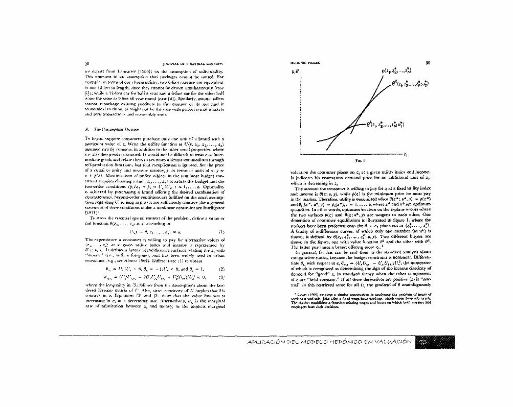
.4. Táe Consnmpttm. Deanm
To begin, mppme consumers parchase, only one «nit of a brand wtth a particular value of &. Write the utility function as V(x, £ ¡ , zZf* • ->**} assumed strif tK roncavr, in addition io the other tmial properties* where x i« ¿'I oíÍHT good* ionsurned, it would not 1«° dülicuít to treat <£ as intermedia t** goods and relate them to yet mon* ultimate commodit**-» through self-pnw'ueiion functions, bul that complication is ignored. Si-t the price tax equal M* imify and measure mcome,y, in term* of tmits cti * : / ** x 4- p(,i). Maximtzatto» of utility subject to (He nonlinear budget «on* stramt require choosing x and ' ¿ , , , , . , 4«i to sattsiv the budget and the hrst*order conditions tyt¿zt «•» & « t',jV„ t m. i , . , , , » , Qpum&Hty t* achieved by purchasing a brand ofTenng the desired combination of characteristics. Second-order conditions are fulfilled on the usual assumptions regarding U, so long %&p{z) h not sutiksentiy concave ;for a general statement of the» conditions under a nonlinear constraint see fntriligator [1971]'
To stre^ the es*entw,l spatial context of the problem, define a value *r bd function #(•?$> . . . , - : „ ; a, JF) according to
The expenditure a consumer is willing to pay for alternative values of ÍSj , . , . ; » ; at a given utility index and income h represented by 0(z; s,.^ It deanes a famüy of indifference surfaces relating the ¿t With •'money** V\ e.. With v foregone), and has been -widely used in urban economics (eg , see Alonso 1%-}). Differentiate ¡1) to obtam
K m ?rz¿£'* > °> K » ™ 3 í ¿ * < ^ an£l ^ * *. (2)
where the inequality in /3j follows from the assumptions about the bor~ drred Hessian matrix of f.' Also, •strict concavity of ¿7 imphe? that Oís concave m -e. Equations Í2) and (3Ni show that the value function is increa*i»g in cf at a decreasing rate. AHemativeiy, $tt h the marginal rate of substitution lietween zt and money, or the implicit marginal
p,6 pi! ) ,Z s ; , . . , ,2n)
É í{2„4 Z¡|}UÍ>
valuation the «onsumo- píaco on «¡ a< a given utiiity index and income. It mdi«tes his reservation demand price for an additi»nai unit of <* which is «iccreastng in «,
The armwnt the coiiíamer » wiiling «o pay for l at a fixed utility index and inwme is 0{z; *,}), while JJ(«) B the minimum price he must pay in the market. Therefore» utility is «naxinássed when <?{«*; «*, j ) •« p{z*) andfi„(«*; «*,>'} «M** )» ' ** •>•• •« B,*h«e«*ai»d<»»Ji«i9ptitmim <|Wii«tities. In other words, optimum ideation on the apiane oec«rs where the two surfaces j>{e) and 0{z; s*,j) are tangent to each other, Q»e dimension of consitmer e<juiiii,ri«»a it ¡ilustra»! in figure I, where the surfaces haw teen projected onto the S> - et plane cut at U*,,,.»i*), A family of indifference curves, of which only one member (at **) » sh«Kvn, is defined by í ( ¿„ «J,. » , «J; s»^). Two different buyer» are shown in the figure,, one with value function 8* and the other with OK The latter purchases a brand oílcríng more £t> *
In general, far less can be >aid than in the standard analysis alxwt • oiMf»r»tl« statics, because the budget constraint is nonlinear. Differ», tiate 0tf with respect to a, 0tt, — {UJU„t - UHUa)jU¡, the numerator oí which is recognised as determining the sign of the income elasticity of demand for "good" zt in standard theory when the other components of j are "held constant." If ail these derivatives »re positive (t, is "normal" in this reMrietcd sense for all»}, the gradient of 0 unambiguously
3 Ixwa tVM®) empkrt* & similar c«nstmcli«n sil aaalyjonf die profeiem of isouet of work m ü tied sale. Jot» oifer & íixtá wzgfr'Sxmr jsaefesge, wtUel* varies iixnn j ^ i izt ji>fc, Tfe# msrfeei «establwHes a fanedo!, njlaíiíif wages ítiiá íteurs m wt*kfe t»3tli vvwfeets s»*i employers hme úucit edsáom.
APLICACIÓN DEL MODELO HEDONICO EN VALUACIÓN
4<> JOURKAi, OF POUTICAl, ROONOMS
inorases as a increases. Additional income always increases maximum attainable utility. Hence iffi(z) is convex and sufficiently regular every-where, we might expect higher income eoasumers to purchase greatei amounts of all characteristics. Only in that ease would it be true thai larger income leads to an unambiguous increase in the overall "quality' consumed, and differentiated products' markets would tend to t i strati lied by income. However, in genera! there is no compelling reason whs overall quality sftould always increase with income, Some component! may increase and others decrease (cf. Upscy and Rosenbluth 1971). B< that as it may, a clear consequence of the model it that the» arc natura tendencies toward market «¡¡¡mentation, in the sense that consumers wilt similar value function* purchase ptndutts with similar specification». Thisr » well-known result of spatial equilibrium models. In fact, the alxwc spec! fkat» >n is very similar m spirit to Tiebou ('» (1956) analysis of the implicit market for neighborhoods, local public goods being the "characteristics' in this case. He obtained the result that neighborhoods tend to be seg menleti by distinct income and taste groups (also, see Kllicfewn 1971) That result holds true for other differentiated products too.
Allowing a parameterútation of taste» across consumer», the utility function may lie written {?(*,, * , , . . . , * „ ; «), where a is a parametci that differs from person to person. Equilibrium value functions depent on both j> and a. A joint distribution Junction F(j, a) is given in thi population at large, and equilibrium of all consumers is characterised bt a family of value functions whose envelope is the market hedonic or ira plicit price function.
The model is easily expanded to include several quantities, so long a consumen are restricted to purchasing only one model. Foltowint Houthakker (1932!, the utility function becomes l/(x¡, et,..., z„ m) where m a die number of units consumed of a model with characteristics i The constraint n j> = x + mp(s), and necessary conditions become
Mi ~ - ~p(i)U, + Um m Q, (4 em
?C _ . . -mp,{z¡Ut + U,t m 0. (5'
The value function is still defined as the amount a consumer is willing t< pay lor z at a fixed utility index but now with the proviso that m is optiiti ally chosen. That is, 0ij> „..., ¿J is defined by eliminating m from
K w UiJ — mff, 4 , , . . . , g„ st)
¡I lit = (I
Again, 0lt is proportional to U.JU,, The logic underlying figure I remain intact, and it can just as well serve for this case. However, seeond-ordei
HSDONK! MtlCBS V conditions are now more complex. For example, convexity of p(s) i» no longer suliieiertt lor a maximum as it was in the case where M was restricted to be unity. Also, it is necessary to employ stronger assumptions than those used abúvv if the. value function 0 is to be concave.
Note there is no question of monopsony involved here. Consumers act wmpetittvely in spite of the fact that marginal cost ofqualíty, fifa), is not necessarily constant—it is mcreaáag in figure I—because as many units as desired of any brand can be purchased without affecting prices. The function p{s) is die same for ail buyers and independent of w,
B. The PntáíctÍM Dtcóim
Having set up the formal apparatus above, we give a symmetrical and consequently brief account of producers' Ideational decisions. What package of characteristics is to tie assembled? Let M(e) denote the number of units produced by a firm of designs offering specification & The discussion is limited to the case of nonjoint production, in which each production establishment within the firm specializes in one design, and there are no cost spiliovers from plant to plant. Thus a "firm" is an arbitrary collection of atomistic production establishments» each one acting independently of the others. Analytical difficulties arising from true joint production are noted in passing.
Total costs in an establishment ¡art C(MX z; $ , derived from mmirow-ing factor costs subject «o a joint production function constraint relating M, z, and factors of production. The shift parameter fi reflects underlying variables in the cost mimtnmrtien problem, namely» factor prices and production function parameters. Assume C is convex with C{0, *} «• 0 and CH and C„ > 0, '¡There are no production indivisibilities, and marginal costs of producing more units of a model of given design are positive and increasing. Similarly, marginal costs of increasing each component of the design are also positive and nonxtereasing, (Ordinarily, there will be some technological constrain» that Hiatt the set of feasible location» on the plane.) Each plant maximitcs profit n «• Mp(z) — C(M, zt , . . .».£„) by choosing M and z optimally, where unit revenue on design «is given by the implicit price function for characteristics, i»(<).4
* <>«r mafeííiíy to tr«at j<«nt production «otitóviaíty yet simply stems fmm the spec» mtm^d-mmmadxttm assamptiaíi, tf & fmttt; number fsay $) ©f packages is available, it would be stnugtw&erwaril fiarmauy t» speciiy a sfcsKtoaW &-c¡a»potMí»t multiple prothie* c«*t faiictittn ibr the firm, aod proceed an that basis. In tfreprescat case, tmm «stgage ta jomt jíTOductídií <«Uy bsdaras iaey own «ttaí»Síthiae«ts sj»eeíalizií in dtñermt aaefeage*. ¡However, geaitiae Joint ístísdaetíG» remitiré» cost de|W«<íe«ei«s berwee» production UBÍKS within the ürm; the arm must choose a fuKC&Kt M{z) 4amtMtt% a« entire "product tirte" «acied ia die market, lite entire fwiicfebn M{z) is an argumeat in each i>laat costs and lf»tai costs "m tsm are the Htm tor íattfgíal) «ver all príiéwaíc*» <sst»blishJ»cnt costs. A c«mi ete tr«atn*cat requires usr of ftmetionsll wwiysis «ad is heysin u»c se*^e of this paper.
APLICACIÓN DEL MODELO r+EDONICO 6N VALUACIÓN
4¿ JOURNAL OF POLITICAH. ECONOMY
Again, firms are competitors and not monopolists even though marginal costs of attributes/>,(£} a ir not necessarily constant because alt establishment* olixrve the same pnces and cannot affect then» by their individual production decisions; ¡i{z 1 is independent of M,
Optimal choice of M and z requires
PÁs) = C,¿M, z„...,s,)¡M, i - l , . . . , « (6)
!>{.z) - C„(M, * „ . . . , Í , ) . (?)
At the optimum design, marginal revenue from addition»! attributes equals their marginal cost of production per unit sold. Furthermore, quantities are produced up to the point where unit revenue p'i) equals marginal production cost, evaluated at the optimum bundle of eharac-tei ¡sties. As above, convexity of C does not assure second-order conditions due io nonlinear»)' o(p{s), and some stronger conditions, assumed to be satisfied in what follows, are required {see Intriligator 1971).
Symmetrical!} with the treatment of demand, define an offer function $(i , £„; it, (J) indicating unit prices (per model) the firm is willing to accept on various designs at constant profit when quantities produced of each model are optimally chosen. A family of production '"indifference" surfaces is defined by ¿. Then <¿>( „ . . . , « . ; it, fi) is found by eliminating ,1/ from
R ~ M4> - CM, zi,,.,, *.) {8}
and
CU(M, zu...,ij - $. (9)
and solving for tp in terms of.;, it, and fi. Differentiate (8) and (9) to obtain <¡>,t = Ct¡!M > ¡t and 0 . = I/A/ > 0.
The marginal reservation supply price for attribute i at constant profit, assumed increasing in z,. is <£,_. Asjain convexity of C does not always guarantee 4>,,,, > 0. Since «4 is the oiler price the seller is willing to accept on design z at profit level jt. while p{s) is the maximum price obtainable for those models in the market, profit is maxirabrcd by an equivalent maxiimwitton of the offer price subject to the constraint fi = $. Thus maximum profit and optimum, design satisfy /»,(>*) *
<¡>.,J.z*,...,4;n*,0), for i * l,...,n, and fi(c*) = 4U* 4; H*. fi'.. Producer equilibrium is characKroed by tangency between a profit-characteristics indifference surface and the market charactcristies-impltctt price surface.
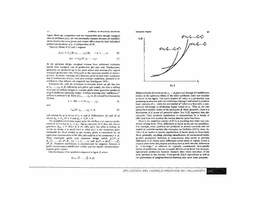
One dimension of the solution is depicted in figure 2, where
¿ ( i , , 4 . • • •, •=»*; n> fi)
HEDOfilO PRICKS +3
P«2».4 «¡»
Fu», i
defines a family ofcurves on t lsei , - $ plane cut through the indifference surface at the optimum values of the other attributes. Only one member is shown in the figure. '1 he curve labeled $* refers to a production unit possessing production una cost conditions making it well suited to produce lesser amounts or*,, while the, one labeled <¡>z refers to a firm with a comparative advantage at producing higher values of « , . That is, the two plants have distinct values of the parameter fi. More generally, there is a distribution of fi across ail potential sellers. Let G(fi) represent that distribution. Then producer equilibrium is characiertwd by a family of offer functions that envelop the market hedonic price functions.
What is the empirical content of fl? It is anything that shifts cost conditions among firms. Thus, differences in factor prices are one possibility. For example, many products are produced in several countries and ace traded on national markets (for examples, see Griiiches 11971], chap. 5). There is no reason to assume equalization of factor prices in these cases. More generally, anything allowing identification of conventional multi-product production functions in cross-section data serves to provoke differences in p. Factor price differences aero» states or regions within a country often serve this purpose and do so here as well. Second, differences in "technology," as reflected by typically unmeasured, firm-specific factors of production, also act as supply shifters across firms. For example, agrtcuitural production function research often treats education of the farm operator in this manner. Hrett-specific R&D expenditure as well as the phenomena of progress-funciion-iearnittg also serve these purposes.
APLICACIÓN DEL MODELO HrEDÓNICO F=N VALUACIÓN
P.<r> f^,4
^djt4....4iij*)
44 JOVRNAt. OF POUTICAl, ECONOMY
C. What Di> lltdenk Prices Ahmt
An answer to the question is an immediate application oí the above analysis Superimpose figure 2 onto figure I, in equilibrium, a buyer and seller ate perfectly matched when their respective value and offer functions "kiss" each other, with the common gradient at that point given by the gtudient of the market clearing implicit price (unction fi'z). Therefore, observations p{z) represent a joint envelope ofa family of value function» and another family of offer functions. An envelope functkijt by itself reveals nothing about the underlying members that generate it; and they in torn constitute the generating structure of the observations. Some qualifications arc necessary however, (a) Suppose there is no variance in fi and ail firm» are identical. Then the family of offer functions degenerates to a single surface, and p(z) must be everywhere identical with a unique offer (unction. Price differences between various packages are exactly equalizing among .sellers because offer functions are constructed at constant profit, A variety of packages appear on products markets to satisfy differences in preferences among consumers, and the situation prnisls because no firm finds it advantageous to alter the quality content of its products, (b) Suppose sellers differ, but buyers are identical. Then the faintly of value functions collapses to a single function uñé is identical with the hedonic price function. Observed price differences are exactiv equalizing across buyers, and p{z) identifies the structure of demand.
HI. Existence of Market Equil ibrium
Analysis of consumer and producer decisions has proceeded on the assumption of market equilibrium. This section demonstrates some details of equilibrium pri< e and quantity determination. Market quantity demanded for products with characteristics z is (^{z'h and Q'(z) is market quantity supplied with those attributes. It is necessary to find a function ¡>{z i such that Q"[z "i — Q",l) for all z, when buyers and sellers act in the manner descrilied above. The fundamental difficulty posed by this problem is that Q*{z) and Q'iz) depend on the entire function p(z). For example, suppose quantities demanded and supplied at a particular location do not match at prevailing prices. The effect ofa change in price at that point is not confined to models with those particular characteristics but induces substitutions and location»! changes everywhere on the plane. A very general treatment of the problem is found in Court (1ÍH1), and our discussion is devoted to some examples, lítese examples have been rhosen for their simplicity but illuminate the problem and illustrate most of the basic issues. Jn contrast to the test of the paper, discussion is specialized to the case where goods are described by exactly one attribute (i.e., « m 1). Therefore i , represents an unambiguous
HKDON-tC PRK3S 45 measure of "quality." When n = I, the location surface degenerate! to a line rather than a plane, and producís are unequivocally ranked by their z content,
A. Shm-Run Efxéibriim
Consider a short-run equilibrium m which firms have geared up for the quality (z,j of goods they can produce and are only capable of varying quantities. The horizon is sufficiently »hort so that new ««try is precluded, and the distribution of firms by quality is given as an initial condition. The market reveals an implicit price function p(zt], and each firm determines the quantity it supplies to the market according to condition (7/. Market supply in a small interval dzl near quality Zj is found b> weighting firm supply by the quality distribution function. Consumers differ in Kistes and income, but all determine optimal quality and quantity as in ,'4/ and {"}]. Market demand near any quality « , is found by using the conditions of consumer equilibrium to transform the distribution of tastes attd income into a distribution of qualities demanded and weighting individual quantities demanded by the resulting distribution of qualities. Finally, setting demand equal to supply yields a differential equation in p and i , that must be satisfied by market equilibrium, subject to some hounditr) conditions.
To be specific, assume that 0'(A', .*} = {al'l\M%z\ for all firms. Also, suppose firms are uniformly distributed by the characteristic z,: fizydz, = *<fc, for £,, s 2, S z,„ where k is a confitan! and «,, and ,;,, arc cxogenously determined upper and lower limits of the product line. Apply equation (7) to obtain firm supply: A/{«,) «• # /«? , since qualities cannot be varied by assumption. Therefore,
9"U,)<b:, = g^WizJiUi = t(i/«)¿(*l3.'.ííJ<fe,. (10)
Assume a fixed number of consumers in the population and that only i a te unit per customer of the optimal model is purchased. Consumers have the same income, and utility is linear i» x and *,, with the marginal rate of substitution, p, varying from person to person- Maximize (/{*, zt) = * + IK, subject toj> = * +/*(*,). Each consumer purchases a brand for which ip¡iz¡ =» jt>'{i|} = p- In this case the value functions of figure ! are straight lines with a different slope, p, for each person. The marginal condition charatierizes consumer choice so long as p" > 0, wfueh will be shown to be true. Suppose p is distributed uniformly, j'tp)4p *> Up for p, ¿ p £ p„ where b is a constant and n, and p, are, respectively, the largest and smallest marginal rates of substitution in the population. Use the marginal condition f «« p to transform f(p)dp into
APLICACIÓN DEL MODELO HBt>ÓN\CO EN VALUACIÓN
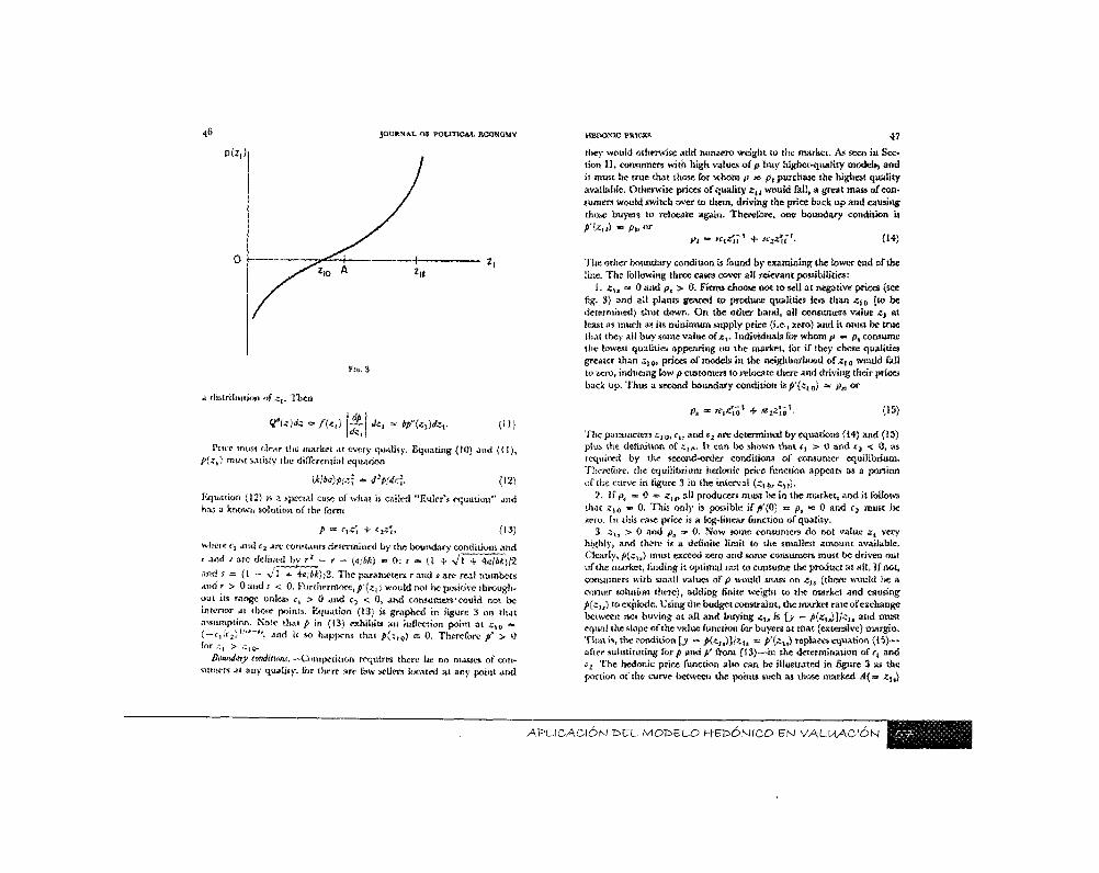
4*» jotsRNAi. o r p o t r neAi . RCOHQMY
Píí | )
0
Fía. %
A distribution of ¿ j . Then
Q'U'li/z = / (* , ) p i (fe, = */fe)<fe,, (11)
Puce musí clear the inarket at every quality. Equating (10) and ( II) , p(,zt) must satisfy the differential equation
{k}ia)ptz\ » ¿^¡dtl (12)
Equation (121 a a special case of what is called "Euler's equation" and has a known solution of the form
p - < • , < + ÍJÍ*,» (13)
wlteie f, and <, are constants determined by the boundary conditions, arid r and t are < i e f i n t^¡_byj^_- ' - (ajik) « 0: r — {I + </l + 4a/M|/2 and Í -» |1 - v t * 4<¡,'M)i2, The parameters r and #are real numbers Amir > Oandi < 0. Furthermore,/>'(«,) would not lie positive throughout its range unless e, > 0 and c, < 0, and consumers* could not be interior at those points. Equation (13) is graphed in figure 3 oil that assumption. Note that p in (13) exhibit» an inflection point at <,„ m {-fi 'rV,""-", and it «> happens that jS(-«o) s 0. Therefore p" > 0 for.;, > J ) S .
Bmuuiittjf tmiitwiu. -Competition requires there be no masses of consumers at any quality, for there are few sellers located at any point and
HEÍJONJO PRICKS 47
they would otherwise aád nomtero weight to the market. As seen in Section II , consumers with high values of p buy higher-quality model») and it must be true that those for whom p m pt purchase the highest quality available. Otherwise prices of quality z¡, would fail, a great ma» of consumers would switch over to them, driving the price back up and causing those buyers to relocate again. Therefore, <mt boundary condition is p'(z„) - p i ,«r
/>< - ««¿¡i" + «*«"«'• <•*)
The other boundary «mditKm is found by examining the lower end of the tine. The following three asm cover ail relevant possibilities:
1. je„ = 0 and p, > 0. Firms choose not to sell at negative prices (see fig. 35 and all plants geared to produce qualities less titan zia (to be determined) shut down. On the other hand, all consumer» value e, at least as much a» its minimum supply price (i.e., ¡tero) and it must be true that they- all buy some value of«,. Individuals for whom p -m pt consume the lowest qualities appearing on the market, for if they chose qualities greater than i 1 0 , prices of models in the neighborhood of xt¡, would fall to ztro, inducing low p customers to relocate there and driving their prices back up. Thus a second boundary condition tep'(etll) •> j»„ or
ft-«t«sól +*i-í>¡1- C«3)
The parameters zia, c„ and <f2 «ire determined by equations (14) and (iS) plus, the definition of ! t i . It can be shown that et > 0 and ¿2 < 0, as required by the second-order conditions of consumer equilibrium. Therefore, the equilibrium Itcdomc price function appears as a portion of the curve in figure 3 in the interval (z, & tif).
'i. 1 f pt m 0 • g, t, all producers must be in the market, and it follows that z%a m 0. This only is possible if ¡>'{0) *» pt •» 0 and r , must be r.ero. In this case price is a log-linear function of quality.
3. zu > 0 and p s =• 0. Now some consumers do not value * , very highly, arid there is a definite limit to the smallest amount available. Clearly, fi{zix} must exceed ssero and some consumers must !>e driven out of the market, finding it optimal not to consume the product at all. If not, consumers with small values of p would mass on 4 ^ (there would be a corner solution there), adding finite weight «» the market and causing plzi,) to explode. Using the budget constraint, the market rate of exchange between not (raving at all and buying z%, is fj> — p(ZtJ]l<t, and must equal the slope of the value function for buyers at that {extensive) margin. That is, the condition \j — pifitMl^u ** ¿'fo») replaces equation (15)— after substituting for js and p" from (13)—in the determination of c, and c2 The hedonic price function also can be illustrated in %ure 3 as the portion of the curve between the points such as those marked ¿1(= ¿ u )
APLICACIÓN DEL MODELO l-ret>ÓNfCO 6N VALUACIÓN • • • • • H i
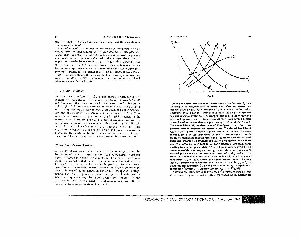
a/> JOt R V t t , OF POt STICAJ. ECONOMY
mil i , ( \<?un f¡ ¿ml <, l i ne lire corra t signs and the. sctond-oreter conditions are lulblkd
A second i\pc of shor! run rquiubtmm amid IK considcied in which cxmins- linns o n -tlttr qualities as well as quantities of their products When theif is a distribution «I etwt ftinttiuns it is ntcrysarv to proceed imlotfoush to lilt treatment ol demand in ihe example above Ioi example, <KH misfht he described t» (a 2 \2zl with / variing across liru s I ht n / 2 — « , / /f is used to itanslorm the distribution of / into a distiihulton ut <jtnl»tti s supplied 1 ht resulting distribution wti^hts firm quammes supplied in ¡he d( lennmaiioti oi nuiktl supply at am quality \ iittlt cvperirnetiUtion ssill show that thr differential equation resulting from seitmi? QJ ¿, « Q'(z% is nonlmeai in most eases, and dosed solutions -in nol ahvass feasible
B I<<¡¿ Run ¡ qintib) urn
I irms inav s,m qualities at Hill and also construct establishments oi optimum M/r \ o entrv rcstr» tiom tiupl) ihr al«< nee «f profit (r* = 01 and lone; tun offer price lor rath firm must satisfv 4>(¿ fi> m
I \l s ft \1 Plants are constructed to produce models ¡>l qualil) e at it uumum cost Hcrwe scale economies arc exhausted under romjwu timi -ind tlie optimum production unit occurs where ( If 5 ft is ¡meat in 1/ vanmoiis uf quantity hung arhieved bs changes m tiie numbci oi establishments l e t A 4 ¡i leprrscnt minimum average cmt ol *fru oxsiablisbimtii o! optimum sue I7ic>i L..M x ft =• Wt z, fi in tlit Umg run Ilitrcfore t> = ft ; p and p • = k i flj is the equiliht urn londuton (or maximum profu and jdtc 1 i« 1 oiupictclv determined bv supph «1 h\ the mvelopr «f the family h<i, fi) with icsptit t<t // Goiciaii/alton to 1» characteristics is obvious in this cast
IV. An Identification Problem
Section III demnnstiatcd that complete solutions (or p 1 and the distiibmiroi of qualities ttaded sometimes can be obtained >! sufficient 1 pruri strut tuic ts 111 posed <m the problem However it is not aissuss fmssible 10 pit» ted m that nunner In gent.nl tin differential equation dc fining / ; is nunhniar and it mas not be possibh to ¡md dosed solu-mm'. Moreosu a gnat chai o) structure must be imposed loreurmplc, tiie distributiun »(income follows no simple lass throughout us rang! niikinsr 11 dilfkuh lo >poih tin problem rnmplt tsh f-inaih pattul-diilerentni equations must lie solved who» their is more than one diaiai ttrisfii Í his station sketches in alternative ^nú morí iffiueiit inoctdur? based on the unalvfis of'sertion II
MBDOSaC! ÍKICES 4 9
fto.4
As shown above, derivatives of » consumer's value function, 6,,, are proportional to marginal ratra of substitution They arc reservation-demand prices for additional amounis of <ef at a constant utility index ITicrefore (0tl(z)} are the inverses of a set of ordinary compensated demand functions lor the i(*s The marginal cost of x, to the consumer n jM*)» a<"' opUnt»! * is determined svhere marginal costs equal marginal «dues One dimension of these marginal concepts is illustrated in figure 4 The curves labeled 0¿ are derivatives of 0* m figure I and reflect compensated demand functions for various buyers The dashed hoe labeled Piiz) »s the common marginal cost confronting all buyers Consumer choice is sjiven by the intersection of demand and marginal cost ft should be emphasized that the functions 0H(s) see compensated demand prices (real income held constant) and ma only be derived once equilibrium is determined, as m Section II For example, a new equilibrium resulting from an exogenous shift in p wouU not als»avs be gjs'cn bv die intersection of the new marginal a » » , ^ {t), and the initial compensated demand pnce fimuions. An exception occurs svfaen 9„. =» 0 and the family of surfaces <*{«, »), such as depicted m figure t, are all parallel to each other 0„„ - 0 is equivalent to constant marginal unitty of money and fl,( w unique and independent of a only in that case If i9„, ft 0, the shape and location of the 0{t functions are determined by the equilibrium conditions of Section H> tangenry between p{t¡ and 0'(z, a*)
A similar procedure applies to arms 0,t is the reservation supply pnee of incremental z¡ and reflects a profit-compensated supply function for
APLICACIÓN DEL MODELO H-5DÓNICO BN VALUACIÓN
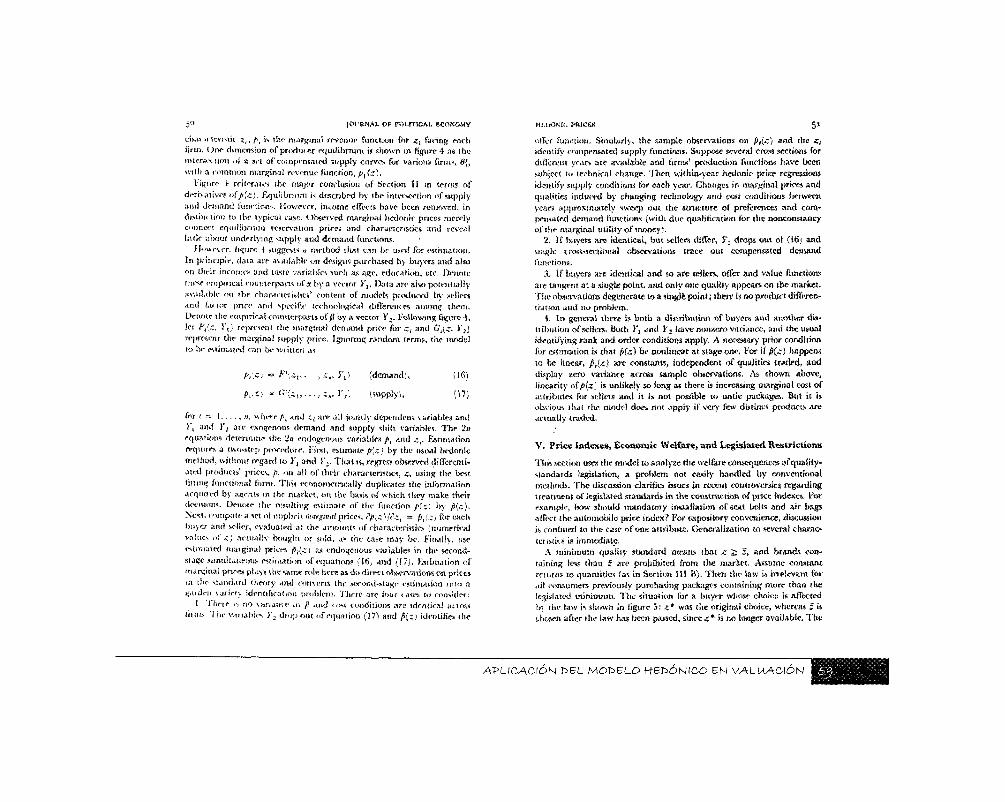
5 o J0< 'RNAl. OF r O L m C A L ECONOMY
chat.Kíei'istie ¿,, / ¡ ( is the marginal rrtcmif function for ¿¡ facing each fino. One dimension oí pnxitnor equilibrium is shown m figure 4 as the intersection ol a irt of compensated supply curves for various firms, 0>, with a common margina! revenue function, /),fa¡.
figure 1- reiterate? ti» major conclusion of Section II in terras of dcrhativos of/(c) . Equlibrnim is described by the inter>ccti»n of supply and dnnand functions. However, income effects have been removed, in distim tion to the typical case. Observed marginal hedonir prices merely connect equilibrium reservation prices and characteristics and reveal bitie about underlying supply and demand functions.
However, injure • suggest? « method that can iw used for estimation. In piinriple, data arc available on designs purchased by buyers and also on their income* and taste variables such as age. education, etc Denote these t-mpmcal counterparts of at by a vector F ( , Data are also potentially available on the characteristics' content of models produced 1A- sellers and fat tor price ami specific technological tlifferctKCs among them. Denote the empirical counterparts of/i by a vector Y¡. Following figure 4, let f',(c, }'¡) represent the marginal demand price for c, and C ((c }',) represent the marginal supply price. Ignoring random terms, the model to be rstiinatrd am be written as
p,\ii = i ? ' ; c ) , . , £„. >'j V (demand), ¡16)
p„Z! - ' í ' í c , , . . . , . : , , )*/, ¡supply), (17)
for i - 1 , n, uJierc pt ami •¡ af(. ¿J] jointly dependent sariables and > i and Y¡ are exogenous demand and supply shut variables. The 2» equation* determine the in endogenous variables j>t and z,. Estimation requites a tuo-siep procedure. First, estimate p[.z> by the usual hrdonic method, without regard to ¥t and I',, That»s, regress observed differentiated products* prices, />, on all of their characteristics, s, using the best littmg functional form. This econometrieally duplicates the information acquired by agents m rhr market, on the basis of which they make their decisions. Denote the resulting estimate of the function p(*; by p(z). Nest, compute a set ol implicit mvgimil prices. <£;.£'./At, = /?,(.; j for each buyer and seller, evaluaied at the amounts of characteristics (numerical values of" 4; aetuallv bought or sold. ,i« the case may be. Finally, « e estimated marginal prices p,(¿ i as endogenous variables in the second-stage simultaneous estimation of equation? (16,. and (I7j. Estimation of" marginal prires plays the same role here as do direct observations on prices in the standard theory and convert» the second-stage estimation into a gatdeti sarirty identification problem. There are four rases to rounder.*
I Theic is no varíame in fi and <mt conditions are identical actos* lit ins ' Ihr variables J", diopout of equation (17) and />(:) identifies the
MLUONK. I»RJCKS 5*
offer function. Similarly, the sample observations on p,(-"l and 'he z, identify compensated supply functions. Suppose several cross sections ibr difieren! years are available and firms' production functions have been subject to technical change. 'liten within-year hedonir price regressions identify supply conditions for each year. Changes in marginal prices and qualities induced by changing technology and cost conditions between years approximately sweep out the structure of preferences and compensated demand functions (with dw qualification for the noneortstaiicy of the marginal utility of money!.
2. If buyers arc identical, but sellers differ, i*( drops out of (18; and single cross-sectional observation* trace out compensated demand functions.
3, If buyers are identical and so arc sellers, offer and value functions are tangent at a single point, atsri only one quality appears on the market. The observations degenerate to a «ingle point; there is no product differentiation and no problem.
1 In general there is both a distribution of buyers and another distribution of sellers, Both K, and fz have nonzero variance, and the usual identifying rank and order conditions apply. A necessary prior condition for estimation is that p(¿) be nonlinear at stage one. For tí j>i¿) happen* to be linear, p¡{¿) are constants, independent of qualities traded, and display «ero variance across sample observations. A* shown above, linearity of fi(z] is unlikely so long as there is increasing marginal cost of attributes fur sellos ami it is not possible to untie packages. But it is obvious that the model does not apply if very few distinct products are actually traded.
V. Price Indexes, Economic Welfare, a nd Legislated Restrictions*
This section uses the model to analyze the welfare consequent» ofquality-slandards legislation, a problem Hot easily handled by conventional methods. The discussion clarifies issues in recent controversies regarding treatment of legislated standards in the construction of price traie&cs. For example, how should mandatory Installation of seat bete and air bags affect the automobile price index? For expository convenience, discussion is confined to the case of oac attribute. Generalization to several charas-tet¡stirs is immediate.
A minimum quality standard mams that i i i , and brands containing less than I are prohibited from the market. Assume constant returns to quantities fas in Section III It), Then the law is irrelevant for ail consumers previously purchasing packages containing more than the legislated minimum. The situation for a buyer whose choice is affected In the law is shown in figure 5: z* was the original choice, whereas i is chosen after the law has been passed, since z* is no longer available. The
APLICACIÓN t>BL MODELO r-fEDÓNICO EN VALUACIÓN
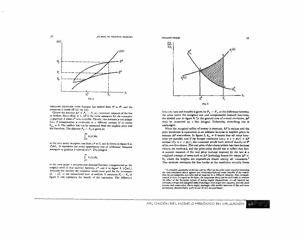
5" JOURNAL OF POLITICAL ECONOMY
minimum attainable value function has shifted fro»» 9' to #*, and the consumer is worse off (see ec¡. {2]),
Choose the distance &P » P: - Px « a monetary measure of the Joss in welfare. Since d6,'Sy •» 1, AP is the bribe necessary for the consumer to purchase 2 when z* was available. Clearly, this measure is not unique (i.e., if compensation is evaluated at A different ¿meant of <r) unless SJ(, w 0. The welfare loss ran be estimated from the implicit price and bid functions. The distance P2 — P0 is given by
Jrt ítt*)*.
or the are.» under marginal COM front e* to 1, and is shown in «¡jure 6 as ¿,«*2, it represents (he social opportunity cost of additional resources necessary to produce i instead ate*. The integral
or the area under a compensated demand function (compensated at the original level of real income) between «* and f in figure 6 («fotf,) mrasures the amount the consumer would have paid for the increment <z, - £*) at the unrestricted level of welfare. It measures Pt - />„ in figure 5 and represents the benefit of the restriction. The difference
HEDaiaC »Ric» 53
it PM)
9Zi
fts.6
between costs and benefits is given by /*j — Pit or the difference between the areas under the marginal coit and compensated demand functions, the shaded area in figure 6. in the general case of several attributes, &f must be measured by a line integral. Otherwise, everything else is unchanged.
When the marginal utility of taortey is constant, AJf is, unique and the price restriction is equivalent to an additive increase in implicit prices in amount AP everywhere. In figure 5, $„ •» 0 means that all value ftmc-lions are parallel» and if the budget constraint was j» m x + p(z) -f &P instead of;» » x + p(z), the consumer would have arrived exactly at S* of his own free choice. The real price of the characteristic h » risen because dicaces are restricted, and the price index should rise to reflect that fact. A natural measure of the real price increase imposed by the law is a weighted average of terms such as &P (mciudmg buyers for whetm AP m 0), where the weights are expenditure shares among ail consumers.* This measure overstates the lost insofar as the restriction actually forces
5 A complete assessment of the law aftd its effect OM the price index requires balancing the costs calculated above against a»y ejuemaiity-itídoced «acial benefits of the restriction. In our judgment, seat hells am! air hags arc in a different category than emissam-control devices. In tegard to the latter, the apparatus above can be used easily to analyze the effect oí the European system of (axing engase displacement. An ad valorem tax mercase* average and marginal easts of packages with larger liter capacity, and the usual ~m<xmc and substitution effects apph/: packages tvtth smaller amounts of tiss and complementary characteristics {such as sue of ear) arc purrhascd.
APLICACIÓN PELMOMLO HBHÓNfCO EN VALUACIÓN ¡JÉMJilli MmUSmUmm
•>\ jot RNAI iW pcmm M foosovry
some < onsuim rs <omplu< h out of the galeae good1» marker since thev IM *pc thr full loss 4/J \Ko( ^tand^rd mdex rtumbtr probíftm a«M whm the marginal utihtv of mone\ i> not constant
\ Í. Conclusions
I lm papa h is dtatvn out the ol*sm mon d tunscqtK rtces of the cmwti uu ni impl¡< it nujkets íot th u^utrnucsemljodied m ddterentntcd pioduct^ When good* cm be ti caled a*, tied packages* of characteristics, observed market p n m ire ateo comparable on those terras fh< «onorau content of thí relit tonyhip hetueen observed prices and olrserved characteristics buosriíA f ídítu ontt pi tu. ddTVrtwts iruo»g Í*OÍKK a i r reef ignited as cqtuh/m*r <bff< ««(<'* for the iltrinitívc packages (ho embody Here, H (hew here T price differences gen» riilv are equalizing onh on the marten and not on Üu ¿\frage i l<na, estimated htdonu pna-charaaemtfis JunctiMits ispjcallv idermK nmhir demmd nor *uppfv lis iact th >se ohvtn -mom are díscnlxrd bv i jomí-envelope function and uñíiot by thomeh*** idcntifv. the strut.ture of (omumer pretcrenctjs and prodtiur icchn logics that generate them
I In iornnl « idly^ tv lomphciuü b^ íhc Iscf that budget comttamts are mmlmear Comcquunh it iv not surpnvmg that jat w<*ik« r theorems than «su*»] apph Hnvvtver, a fea-iblc <ronom<tnr procedure U/t esti mating the underlying generating structure has been derived through tht Use oí derivative írattóiormabom When constraints are nonhmir, murgimil prices serve the same role as average pnces do m the linear easc finally» the tsMiitiai fcp&nal context of (hi problem meam that <tuU*tuuuou and íwnmr eíTeus must l>e more cardutlv distinguished lhan mini Indtcd, hen is i majar practical mvUntí, where compfrtsattd d emitid and supph íunctions become the relevant iund&nterjial concqHs Ihtic compensated functions i t? estimated h) thx tumom&tnc method (mé measuieí* of consumer arid producer surplus can be derived directly from thtm He am tópate that the ixtste conceptual framework outlined tbove wiii Imc i vtrutv of apphí ííiuns to rtimv pnuical problems involving tquthbrmnt m * rovs S<*-UOR dat^
i !¡e an IKMS has been -amplified b \ aMummajdíviSiíhditv in production» i^en*i-ih/dtiO! In*, to ¡moiporate nonronvexttHs, and dts<oniinutues nnnt fesult When ru»ncon\ewtws ire not small relative to the market, if is obuou* that onh iwiatcd locations on the characteristics sudacc will in tilltd In o t b r words suth a generah/ation wtil n^turaUv ttirorporite th< <i*e r»| monopfihstsc compt ttuon, and observed "distance" hn terms of ehaiatttnsucsO Íx.Lwecn difTercntiated products will be endogenous.lv deti rrnmed Í he methods emploved above do not earrv through beca i we teitam nonnwr^uiai dt colons tuu*t f*e analyzed, and f*tr more sophist i ( ited techmemes are reqiured
HFDOMG PRtCFS 55 References
Monzo, WdhAin Lúcatmn and Land U&? Cambridge, Ma^ Harvard Uaiy lh$%&t
mA Becker, Gary S **A Theory of the Allocation of Time " Ecm J 75 (September
|%3( 493-517, Court, ljam$ M '^treprenteunal aííd Consumer i>mitrid fhecmes far Cem-
moduy Spectra" EewamttMu % «o 1 (April 1941) 135-62, no 2 (July-Octobrr i*HJ5 241 ^7
Eíheksorí Bevan * Jurisdictional Fragmentation a«d Residciittal Choice" A£L8 61 iMa^ 1971) 334 39
tíordow Robert J 4 l^ic Measurement of Durable Goods Prices-,f Mímosgraphed. Nat Bur hcon Res r Í973
Oniichc*, ¿\t, cd Prue itxkxei una $mlity Ch&ngt Cambridge^ Mass Harvard LÍÍÍV Prfss 1371
Houthakker H 2* Compensated Changes m Quantities »nd Qjjalmes Consumed " Ra hem Siudm \% m. % (m¿) 155-M.
ín¡trilti?ttoT, Michael D Motknmtwé Qpitm&tUw m4 famwm Tfawy Pngicwood Ciiiís NE } Prentice-Hall* 1971
Ixdncasier KcKmJ "A New Approach to Consumer Theory " J <P h 74 {April
Lewr(S»H Gregg 'Iiateres del empleador e» las horas de Trabajo del empleado" (Employer interests in emplxiyee hours of work| Cuadernos 4g heomma* Othoítc \ niv Chile, 1969
Upsev, Richard O and R^erablutb, GtdeoK A Coninbuiion to the New JDe-mand Theory A Rehabilitation of the Gi0e« Good " Camtdtm */* Ecm* 4 Mav 1971} I3I-W
Muth, Richard F i,hHo«seiidd Fraductiod and Qonaumer Demand Function* M
i^mmetrm 34 U«ly 19WS) 69»-708» ObtafMafeoto and GTiiichcs,7M "Makes and Depteciatumm the i- S faiseager
Car Market ** Mimeographed. Harvard \<m\ , 1972 Ijcbout, Charles M "^ l*ure rtteor) of tocalExpenditure" J/* J b4 {<Xtober
1956} 416 ¿4
APLICACIÓN D6LMOI>£LO f-+eC>ÓNICO BN VALUACIÓN
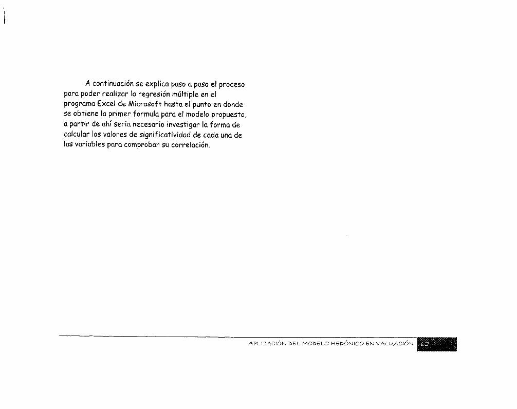
A continuación se explica paso a paso el proceso para poder realizar la regresión múltiple en el programa Excel de Microsoft hasta el punto en donde se obtiene la primer formula para el modelo propuesto, a partir de ahí seria necesario investigar la forma de calcular los valores de signif icatividad de cada una de las variables para comprobar su correlación.
CION DEL MODELO H"EE>ONICO BN VALUACIÓN
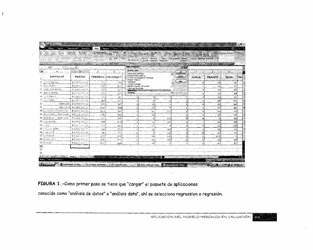
,% , & j * y» fije*
i , ¡ «-se* t Í « ; l*'",- Í
á .. . J. ~ , „ , „ . , * „„„ , ,™^, ,, J, ,> KflW-<Kl •VWtíí.»
J ^ l Z l - * -- - - • - - j •" ~ - ^ = - "áfífC- ¡-U-?*-' va -v• i^^
"•" . " ' * : k . — ™ — : -, — \ . -.:.:., ... « w a w » » ^ ' J " - - * -
r^'^faaá-.«iM».i;Mi!
I Z O N A « K 6 M T S
£
FISURA l.-Como primer paso se tiene que "cargar" el paquete de aplicaciones
conocido como "análisis de datos" o "análisis data", ahí se selecciona regression o regresión.
APLICACIÓN T>6L- MÓCELO HEDONICO BN VALUACIÓN
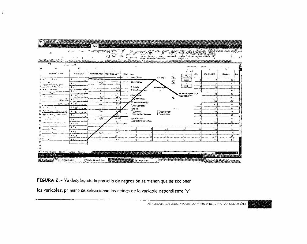
C1*-- W^^»^3^9^^ ^iiwuVKi j j ««• y
f í i iSf i í i iB
FISURA 2 . - Ya desplegada la pantalla de regresión se tienen que seleccionar
las variables, primero se seleccionan las celdas de la variable dependiente "y"
APLICACIÓN DEL MOÜELO HEDONICO EN VALUACIÓN
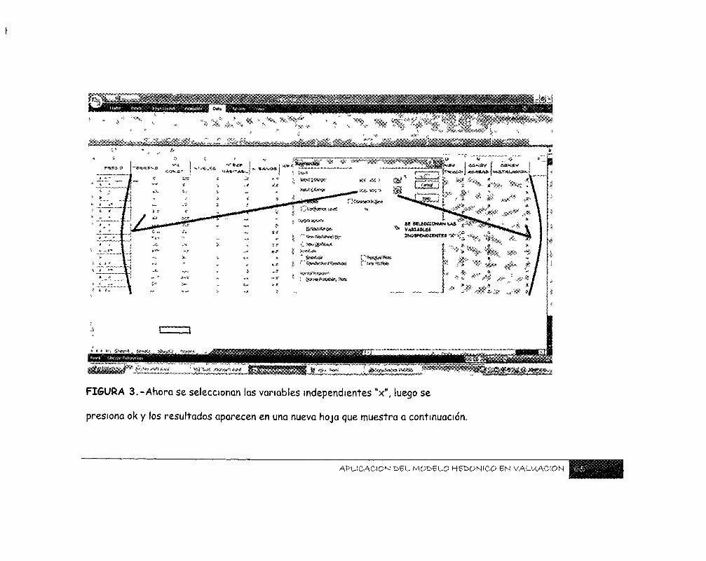
•'j ' 'tf3i*itl>**.*t0*?
>'^\ •tA&Mtá 'v¿*séfe JSawd fiiiifi V^c'i'fi'i'fJfe»..
. « « W O M W M ¡¡ * VAMMUM
í *
í P*^»s»»
í — " 1
...*..*.. y..&*gff*« frfogsl... frhefrti „
.9Ji* J*^*?? J B
FIGURA 3.-Ahora se seleccionan las variables independientes "x", luego se
presiona ok y los resultados aparecen en una nueva hoja que muestra a continuación.
APLICACIÓN DEL MODELO HBt>ONICO EN VALUACIÓN
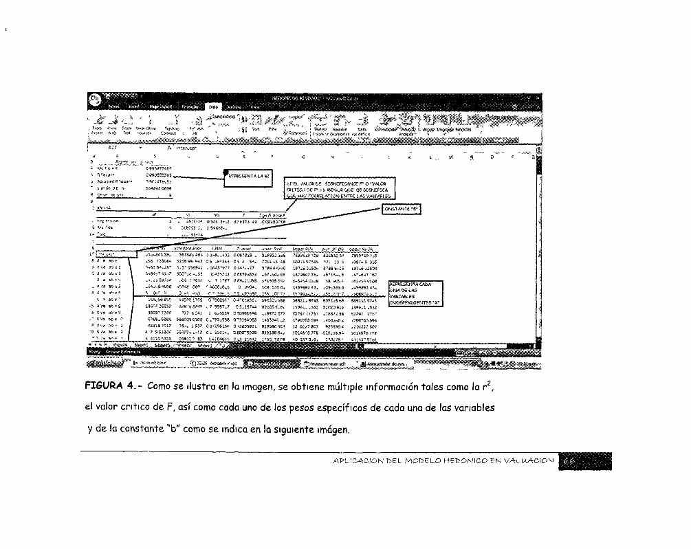
ÜC" Jt * 'JF" ":^':í j--^'^|J^^í|,,v***¡-:';
_ f «SESéNMUK 1
«STÍCO D6 P f» W * ( 8 QUE OS SESMtMM
7 Í J •gg^ w * ^
íSíeí ! » f $2% tJC&t? &5*S <>»•» §< 0 i>p&er*¿&^ DV
« SÍ 8 ac e
s x va a** e ¿
5 X ¿a as e 3
x a s i sM
*. % ¿a a$ e 5
* a see ' "
6 Sí vs a s * 9
i " *Y3 35 « r
S j»vs as i - ',
"3 v / ? a&« j
<^6384»28'"
S&33&463 S2*S t_433
v,fo5 ? S&3ÍÍ ^ i Sis'*
* 5 « £ 0SQ r-400g¿g tS
3 -*1 ¿-ÍO - T " > i ,
0$ ¿ 5**
008234834
O 0**04..
P 5 *g*>9£-
mssz isa
3**8$4»5
JW OC 7j-
7g$55i9 ? Í9
i89?4$75SÍ*
i9Ti.S 3¿5ÍÍ*
i&74&<S? ?§¿
2 M « 26852
3803 ? 73SS
CH«.$8S6
¿331*7CC7
•i 7 «¡£.5836
9*5*0 i Í5& -CMS»"»
5S8"'» gá<3<í Í . 7 9597^7
327 fi24í £ &55S9
5S6O09G3C0 C Í T 9 S Í , 5 S S
^S-* ; «37 S 572<?&ÍSfi
C5*157«
Q"&84963
0 7.2*08931
*¿M?Í 577
933550*04
&2SS3¿ S*
*<J1 Í5 i
38521**743
139***. -531
527S7 H757
2790705 594
735 5* 1» 7*3
1S7¿6 5Í504
.^ ' ' -647 "«2
^ Q g S ^ . ^ 2 ...
3 «S i l l 37¿3
1S<U«1 «-5J2
52??7 ITS'»
fc79ír08 S54
at032? 807
ÍÍJÍ467S 778
í¿teAt3&lA3
HUB**!*
FIGURA 4.« Como se ilustra en la imagen, se obtiene múltiple información tales como la r2:,
el valor critico de F, así como cada uno de los pesos específicos de cada una de las variables
y de la constante "b" como se indica en la siguiente imagen.
APLICACIÓN V>BL- M O T I L O HBDONICO BN VALUACIÓN
APLICACIÓN DEL hAOUBLO HBT>ON\CO BN VALUACIÓN