expenditure spillovers and ﬁscal interactions: empirical

e

n

es. Wethe

res-entativeundingby thetweenulations

ents for

overn-culturalce the

away

Journal of Urban Economics 59 (2006) 32–53www.elsevier.com/locate/ju

Expenditure spillovers and fiscal interactions:Empirical evidence from local governments in Spai

Albert Solé-Ollé∗

Departamento d’Hisenda Pública, Facultat de Ciències Econòmiques, Universitat de Barcelona,Avda. Diagonal, 690, Torre 4, Pl. 2a, 08034-Barcelona, Spain

Received 11 January 2005; revised 26 July 2005

Available online 1 December 2005

Abstract

The paper presents a framework for measuring spillovers resulting from local expenditure policiidentify and test for two different types of expenditure spillovers: (i) “benefit spillovers,” arising fromprovision of local public goods, and (ii) “crowding spillovers,” arising from the crowding of facilities byidents in neighboring jurisdictions. Benefit spillovers are accounted for by assuming that the represresident enjoys the consumption of a local public good in both his own community and in those surroit. Crowding spillovers are included by considering that a locality’s consumption level is influencedpopulation living in the surrounding localities. We estimate a reaction function, with interactions belocal governments occurring not only between expenditure levels, but also between neighbors’ popand expenditures. The equation is estimated using data on more than 2500 Spanish local governmthe year 1999. The results show that both types of spillovers are relevant. 2005 Elsevier Inc. All rights reserved.

Keywords:Local expenditures; Budget spillovers; Spatial econometrics

1. Introduction

Expenditure spillovers are a widespread feature of many services provided by local gments. For example, commuters use roads, public transportation, and recreation andfacilities in their working communities. Air pollution controls and sewage treatment enhanenvironmental quality of neighboring jurisdictions. Radio and TV broadcasts can be seen

* Fax: +34 3 4021813.E-mail address:[email protected].

0094-1190/$ – see front matter 2005 Elsevier Inc. All rights reserved.doi:10.1016/j.jue.2005.08.007

A. Solé-Ollé / Journal of Urban Economics 59 (2006) 32–53 33

ins inurban

feder-llovers, Arnottrs, andimalause aaking., mainlyt also

0]).ramleyrs inmpir-

dituress that

es theprob-ers inalyses

for in-e, Case

esultse Losgiventhan at

ademicvern-reforevern-

e localpapers

ded. Thernmenty to taxbetween

rlog and

betweennd Case

[33] and

from the local border. Educational and job training expenditures may lead to productivity gaworkplaces outside the community. These spillovers have played an important role in theeconomic literature on local government. Its significance is widely recognized in the fiscalalism literature, but most of the papers in this tradition simply assume the existence of spiand analyze their consequences. See, for example, Brainard and Dolbear [9], Pauly [30]and Grieson [3] and Gordon [20], for the efficiency consequences of expenditure spilloveOates [29], Boskin [8] and Conley and Dix [16] for the implications for the design of optfederal structures. The general conclusion of this strand of literature is that spillovers cdivergence between private and social benefits, and thus lead to suboptimal decision-m1

Some authors have also worried about the equity consequences of expenditure spilloversin the context of the demise of US city centers (see Ladd and Yinger [26], for example), burelating to the design of ‘needs-based’ equalization grants (Le Grand [27] and Bramley [1

However, some skepticism remains about the scale and importance of spillovers (B[10]). This may be due to the lack of empirical studies verifying the existence of spillovethe provision of local public services. Weisbrod [37] and Greene et al. [21] are classical eical studies on this topic. The former estimates the extent to which local school expenprovide benefits to other communities via the migration of educated population. He findschool expenditure is lower in states with high rates of out migration. The latter quantifimagnitude of local benefit spillovers in Washington DC, confirming the importance of thelem. Other papers include those by Bramley [10], which quantifies the magnitude of spillovrecreation services provided by English local governments, and Haughwout [23], which anexternalities between suburbs and central cities in local infrastructure policy.2

More recently, some papers have performed new tests of budget spillovers by lookingteractions between the expenditure levels of neighboring communities. See, for examplet al. [15] and Baicker [4] for an analysis of spillovers in state spending.3 However, the onlystudy of this type using local government data is the one by Murdoch et al. [28]. The rof this paper confirm the strength of interactions among local recreation spending in thAngeles metropolitan area. The lack of local expenditure interaction studies is striking,that spillovers are generally expected to be more pronounced among local governmentsthe state level. In fact, as mentioned above, one relevant policy question which fueled acinterest in expenditure spillovers was that of the organization and financing of local goments in metropolitan areas (Greene et al. [21]). The first purpose of this paper is theto fill this gap and provide empirical evidence on expenditure spillovers among local goments.

The second purpose of the paper is to be more precise about the exact nature of thservices analyzed and the type of spillover involved. The modeling strategy of previous

1 In the case of positive spillovers, social benefits are higher than private ones and the service is underprovigeneral policy prescribed for dealing with this problem is a matching grant provided by a higher layer of gove(Dalhby [17]). Other possible methods for internalizing spillovers are boundary reforms, assignment of capacitnon-residents, voluntary agreements, and the creation of a higher tier of government that enforces co-operationcommunities (Haughwout [23]).

2 There is also an independent strand of literature providing evidence on externalities in crime prevention (FuMehay [19] and Hakim et al. [22]).

3 These papers can be included within a broader strand of empirical literature analyzing strategic interactionssubnational governments (see Brueckner [12] for a survey), but most of them focus on tax interactions (Besley a[5], Brett and Pinkse [11], Buettner, [14] and Brueckner and Saavedra [13]) and welfare competition (SaavedraFiglio et al. [18]).

34 A. Solé-Ollé / Journal of Urban Economics 59 (2006) 32–53

th fromn func-rived,rs andin the

rvices.rviceseouslypirical

es ofods,bor-r theopula-

hbor’svariatesnditurehbor’salization

ctionsres anders—a onfor the

ion, wers andre anden in the

ers.of thetions,stinghereoods,g ofality. If

ainderirical

on spending interactions is to consider that the representative resident obtains utility boexpenditure in the community of residence and in the neighborhood. This allows a reactiotion for expenditure in one community vis-á-vis expenditure in other communities to be dewhich can be estimated after controlling for other variables (e.g., population, cost drivepreferences in the community itself). However, although this strategy may be appropriatecase of pure (non-rival) public goods, it may be not useful in the case of congestible seIn the case of commuting spillovers, for example, residents in one community enjoy seprovided by others (e.g., roads, parks and other recreation facilities) but they simultancrowd these facilities. This second effect has not been taken into account in previous emanalyses.

Therefore, following on from Conley and Dix [16] we shall differentiate between two typexpenditure spillovers: (i) “benefit spillovers,” arising from the provision of local public goand (ii) “crowding spillovers,” arising from the crowding of facilities by residents in neighing jurisdictions. The introduction of crowding spillovers in the model has implications fospecification of the expenditure reaction function, since the neighbor’s covariates (e.g., ption, cost drivers) should now also be included in the equation. Failure to control for neigcovariates may result in false inferences. Given that the neighbor’s expenditures and comight be correlated, the omission of these variables will result in biased estimates of expeinteraction effects. It may also be interesting in itself to ascertain the effects of the neigexternalities on local spending, as the estimates may help to design ‘needs-based’ equgrants (Bramley [10]).

In short, the paper will estimate expenditure reaction functions, searching for interabetween expenditures of neighboring governments and for interactions between expendituother neighbors’ covariates. The results will shed light on the strength and type of spillov“benefit spillovers” and “crowding spillovers.” The equation will be estimated using dattwenty eight metropolitan areas and more than 2500 Spanish local government bodiesyear 1999. The remainder of the paper is organized into four sections. In the next sectpresent the theoretical framework that allows us to account for the two types of spillovederive the empirical predictions. This is followed by a discussion of the estimation proceduthe data set used, and by a presentation of the results. Some concluding remarks are givfinal section.

2. Theoretical framework

Following on from Conley and Dix [16], we identify two main types of expenditure spillovOn the one hand, there are spillovers of local public goods, which occur when a fractionlocal public good produced in one jurisdiction is used by residents in surrounding jurisdicand is a perfect substitute for their own provision of public goods. Radio or TV broadcais a good example of this category, which we will henceforth name “benefit spillovers.” Tare also “crowding spillovers,” which are not a consequence of the provision of public gbut from the crowding of facilities by residents in neighboring jurisdictions. The crowdinmuseums and parks by commuters and other visitors is a typical example of this externthe good is congestible, both types of spillovers could appear at the same time. In the remof this section, we will develop a theoretical framework in order to differentiate the emppredictions arising from the two different types of spillovers.


ach hast

ntative

vices

ent’seforeless of

ide it.

od.second

unitywding

ors

. The.one.ed by ahowffect ofidents

analysisenters

2.1. The nature of spillovers

For illustrative purposes, we assume that communities are located on a line, so that etwo neighbors, one on each side. We henceforth denote a community withi, and its left and righneighbors withi − 1 andi + 1, respectively. The neighbors ofi − 1 will be i − 2 andi, and thoseof i + 1 will be i andi + 2, and so on, as shown in the following simple diagram:

“Benefit spillovers” are modeled by assuming that the public goods enjoyed by the represeresident ini (zi ) are the (weighted) sum of those provided by his community of residence(zi)

and by its neighbors. For the moment, we allow utility to be derived only from the serprovided by first-order neighbors (zi−1 andzi+1). Therefore

zi = zi + θ(zi−1 + zi+1), (1)

whereθ is the weight of public goods provided by neighbors in the representative residconsumption. We assume thatθ is a constant and is equal across communities. We are theranalyzing a symmetrical case, in which spillover flows are of the same magnitude regardtheir direction.4 Once this assumption is made, it is also easy to accept thatθ 1, which meansthat people tend to consume more public goods in their jurisdiction of residence than outs

With congestion, the provision technology of the public good may be represented as:

zi = z(Ei, Ni , ci), (2)

whereEi is expenditure,Ni is the number of consumers of public goods andci is a cost driver.The signs of the derivatives are clear-cut from the literature; we should expectzE > 0 andzc < 0,while zN = 0 in the case of a pure public good andzN < 0 in the case of a congested public goTo derive some of our results we use a linear provision technology, so we assume that thederivatives of this function are zero.

Let us now suppose that the residents of a community visit each neighboring commto consume its public goods as well as consuming in their own community. These “crospillovers” may be accounted for by assuming that the number of consumers ini is a (weighted)sum of the population ini (Ni) and that of its neighbors. We consider only first-order neighb(Ni−1 andNi+1). Therefore

Ni = Ni + δ(Ni−1 + Ni+1), (3)

whereδ is the weight of neighbors’ population in the number of public good consumersnumber of consumers in the neighboring localities (Ni−1 andNi+1) is computed in a similar wayAs with θ , we assume thatδ is a constant, is equal across communities and is lower thanThis means that the congestion introduced by a non-resident is lower than the one causresident. The parametersθ andδ need not be equal (although the empirical evidence might sthat they are indeed equal). We introduce these two parameters in order to analyze the etwo different sources of externalities. These are “benefit spillovers,” which occur when res

4 We understand that this is a simplification needed to keep the analysis tractable. However, in the empiricalwe will allow for different interaction coefficients depending on the rank of the city in the urban system (i.e. city cvs suburbs).


andand

of both

e,ulation:

xclusion

atterrs”ulation

e and

o our

) in (4).be able

b-

in one community obtain utility from the provision of public goods by other communities,“crowding spillovers,” which occur when residents in one community visit its neighborsconsume public goods therein. This specification allows for the simultaneous occurrencekinds of spillovers and also for the appearance of only one externality type.

By substituting (3) in (2) and the result in (1), we obtainzi as a function of own expenditurcosts and population, one spatial lag of expenditure and costs, and two spatial lags of pop

zi = z(Ei,Ni + δ(Ni−1 + Ni+1), ci

)+ θz

(Ei−1,Ni−1 + δ(Ni−2 + Ni), ci−1

) + θz(Ei+1,Ni+1 + δ(Ni+2 + Ni), ci+1

)= z(Ei,Ei−1,Ei+1; Ni,Ni−1,Ni+1,Ni−2,Ni+2; ci, ci−1, ci+1). (4)

The derivatives ofzi with respect each of these variables are:

∂zi

∂Ei

= zE > 0,∂zi

∂Ei−1= ∂zi

∂Ei+1= θzE 0,

∂zi

∂Ni

= zN(1+ 2θδ) < 0,∂zi

∂Ni−1= ∂zi

∂Ni+1= zN(θ + δ) 0,

∂zi

∂Ni−2= ∂zi

∂Ni+2= zNθδ 0,

∂zi

∂ci

= zC < 0,∂zi

∂ci−1= ∂zi

∂ci+1= θzC 0. (5)

There are two kinds of testable hypotheses that can be devised from these results: ehypotheses and hypotheses on the size of the coefficients of different variables:

Exclusion hypotheses. Note that expression (4) holds when both types of spillovers m(i.e., if θ > 0 andδ > 0). It is interesting to note, however, that when only “benefit spillovematter, neighbor’s expenditure and costs affect the level of services, but second-order popdoes not. That is, ifδ = 0 butθ > 0, we have:

∂zi

∂Ni−2= ∂zi

∂Ni+2= 0 and zi = z(Ei,Ei−1,Ei+1; ci, ci−1, ci+1; Ni,Ni−1,Ni+1). (6)

When only “crowding externalities” matter neither the first-order neighbor’s expenditurcosts nor the second-order population have an effect on the service level. That is, ifθ = 0 butδ > 0, we have:

∂zi

∂Ei−1= ∂zi

∂Ei+1= ∂zi

∂Ni−2= ∂zi

∂Ni+2= ∂zi

∂ci−1= ∂zi

∂ci+1= 0 and

zi = z(Ei; ci; Ni,Ni−1,Ni+1). (7)

When neither “benefit spillovers” nor “crowding externalities” are relevant we are back tbasic specification of the service level

zi = z(Ei; ci; Ni). (8)

Note that expression (8) is nested in expression (7), expression (7) is nested in (6), and (6By estimating this equation and testing simple exclusion hypotheses one may thereforeto ascertain which kind of spillover (if any) matters.

Hypotheses on the size of the coefficients. Note from (5) that the effect of a variable (in asolute value) decreases with distance, provided thatθ 1 andδ 1. That is, the effect ofEi+1


erallyecifiedsented

n

utilitybudget

d

ain the

mmu-

as

s

(Ei−1) is lower than that ofEi , the effect ofci+1 (ci−1) is lower than that ofci , the effect ofNi+2 (Ni−2) is lower than that ofNi+1 (Ni−1), and this latter effect is lower than that ofNi .Moreover,θ coincides both with the ratio between the effects ofEi+1 (Ei−1) andEi , and withthe ratio between the effects ofci+1 (ci−1) andci :

θ = ∂zi/∂Ei+1

∂zi/∂Ei

= ∂zi/∂Ei−1

∂zi/∂Ei

= θzE

zE

= ∂zi/∂ci+1

∂zi/∂ci

= ∂zi/∂ci−1

∂zi/∂ci

= θzC

zC

. (9)

And onceθ is known,δ can be calculated as follows:

δ = θλ

θ − λ, whereλ = ∂zi/∂Ni+2

∂zi/∂Ni+1= ∂zi/∂Ni−2

∂zi/∂Ni−1= zNθδ

zN(θ + δ)= θδ

θ + δ. (10)

The problem with this testing methodology is that data on the level of service is not genavailable to the researcher. A solution to this problem is to embed equation (4) in a fully spmodel of expenditure determination. As we will see in the next section, the hypotheses prein this section can also apply to this expenditure equation.

2.2. Local government expenditure

We assume that a representative resident of communityi derives utility from the consumptioof a composite private good(xi) and the public service(zi ):

V (xi, zi; bi), (11)

wherebi is a preference shifter. The problem of the local government is to maximize theof the representative resident (11) subject to the technological constraint (4) and to theidentity of the representative resident:

yi = xi + (Ei − Gi)τi, (12)

whereyi is the exogenous income of the representative resident,Gi is unconditional grants another exogenous revenues of the local government,(Ei − Gi) is tax revenues, andτi is the shareof taxes paid by this representative resident. By substituting (4) and (12) into (11), we obtindirect utility function

V (Ei,Ei−1,Ei+1; Ni,Ni−1Ni+1,Ni−2,Ni+2; ci, ci−1, ci+1; τi; yi + Gi.τi; bi). (13)

This function relates the level of utility to the expenditures on public goods made by conity i(Ei) and its first-order neighbors (Ei−1 andEi+1), to the population ofi (Ni) and variousspatial lags of this variable (Ni−1, Ni+1 andNi−2, Ni+2), to the cost variables ini (ci) and itsneighbors (ci−1 andci+1), and to the tax-share(τi), extended income(yi +Giτi) and preferenceshifters(bi) of the representative voter.

Communityi choosesEi to maximizeV , taking the expenditures made by its neighborsparametric. The F.O.C. for this problem is:

Γ = −Vxτi + V z

∂zi

∂Ei

= 0. (14)

Implicit in expression (14) is an equation relating expenditure ini to all the other variableincluded in (13):

Ei = f (Ei−1,Ei+1; Ni,Ni−1,Ni+1,Ni−2,Ni+2; ci, ci−1, ci+1; τi, yi + Giτi; bi). (15)


include

ing froma

riables.logy

g

. This)

s as)

ession

,

atterers”

k[6]):

This expression says that in the presence of spillovers, the expenditure equation shouldneighbors’ spending levels (Ei−1 andEi+1) as well as neighbors’ populations (Ni−1 andNi+1)and neighbors’ cost drivers (ci−1 and ci+1). Moreover, in the case of population (but notthe case of spending and cost variables), the equation should contain information cominmore distant (second order) neighbors (Ni−2 andNi+2). To be more precise, one must performcomparative static analysis of (14) on the testable hypothesis regarding the sign of these vaThe impact onEi of the change in one of the variables coming from the provision techno(denoted byα) is given by the following expression:

∂Ei

∂α= −∂Γ/∂α

Ω, (16)

whereΩ = ∂Γ/∂Ei is the S.O.C. and must be negative for a maximum. The sign of∂Ei/∂α

therefore depends on that of∂Γ/∂α. The expression of∂Γ/∂α is obtained by totally differencin(14):

∂Γ

∂α= −Vxzτi

∂zi

∂α+ V zz

∂zi

∂Ei

∂zi

∂α+ V z

∂2zi

∂Ei∂α. (17)

The sign of this expression is crucial for the results of the comparative static analysissign is clear-cut if we assume that the provision technologyz(·) is linear. Then expression (16reduces to:

∂Ei

∂α= −τi(∂zi/∂α)φ

Ω, (18)

where

φ = −Vxz + V zz(Vx/V z). (19)

In reaching (19), the F.O.C. in (14) is used in order to eliminate∂zi/∂Ei in (17). Note thatφ < 0 whenx is a normal good. This condition ensures that the MRS expression declinexincreases holdingz fixed, which is required forx to rise with income. The key implication of (18is that∂Ei/∂α has the sign opposite to that of∂zi/∂α. For example,Ei falls whenEi+1 (Ei−1)

rises. This result is rather intuitive: the effect ofEi+1 (Ei−1) on Ei should be negative in thcase of a positive externality, indicating “free-rider” behavior. Another implication of expre(18) is thatEi rises whenNi , Ni+1(Ni−1), Ni+2(Ni−2), ci andci+1(ci−1) rise.

Note also that, since the expression of∂Ei/∂α is that of∂zi/∂α multiplied by a factor (i.e.by −τiφ/Ω), the same hypotheses that were valid for thez(·) are equally valid forE(·):

Exclusion hypotheses.Note that expression (15) holds when both types of spillovers m(i.e., if θ > 0 andδ > 0), but comparative statics suggest that when only “benefit spillovmatter,δ = 0 and the coefficient onNi+2 will be zero. Then expression (15) becomes:

Ei = f (Ei−1,Ei+1; Ni,Ni−1,Ni+1; ci, ci−1, ci+1; τi, yi + Giτi; bi). (20)

And when only “crowding spillovers” matter,θ = 0 and then the coefficients onEi+1 (Ei−1),ci+1 (ci−1) andNi+2 (Ni−2) will be zero. The coefficient onNi+1 (Ni−1) will still be differentfrom zero. In this case, expression (15) becomes:

Ei = f (Ni,Ni+1,Ni−1; ci; τi, yi + Gi.τi; bi). (21)

Of course, if none of these types of spillovers matter, thenθ = 0 andδ = 0, and we are bacto a traditional expenditure equation, without any spatial effects (Borcheding and Deacon

Ei = f (Ni; ci; τi, yi + Gi.τi; bi). (22)


0), andthere-

e-n of the

e

eitureed fromndi-uld be

iven thewith

e(15),r”

ill

etest,

g

ith the

iveneffectse first

Note that expression (22) is nested in expression (21), expression (21) is nested in (2(20) in (15). By estimating this equation and testing simple exclusion hypotheses one mayfore be able to ascertain which kind of spillover (if any) matters.

Hypotheses on the sign and size of the coefficients. There are three different kinds of hypothses of this type that can be tested. First, there are some hypotheses that refer to the sigdifferent variables. The results in (18) show that the sign ofEi+1 (Ei−1) should always be thopposite of that ofNi+1 (Ni−1), Ni+2 (Ni−2) and ci+1 (ci−1). This result derives from twofacts: first, the effect of these variables on the level of servicez (see the derivatives in (5)) is thopposite to the one ofEi+1 (Ei−1), and second, the sign of all the variables in the expendequation is the opposite to the one in the provision technology equation (as can be check(18)). Therefore, the validity of the “spillover” model rests not only on the sign of the expeture interaction but also on the fact that the interaction with other neighbor’s variables shothe opposite to the one obtained for the expenditure.

Second, there are the hypotheses related to the relative size of the parameters. Gassumptions ofθ < 1 andδ < 1, the effect of a variable in Eqs. (15), (20) and (21) decreasesdistance. This means that the effect ofNi+2 (Ni−2) should be lower than that ofNi+1 (Ni−1)

and the effect ofci+1 (ci−1) should be lower than the effect ofci . In fact, the ratio between thdifferent lags of a variable provide information about the magnitude of the spillover. In Eq.the ratio between the effects ofci+1 (ci−1) andci provides an estimate of the “benefit spilloveparameterθ :

θ = ∂Ei/∂ci+1

∂Ei/∂ci

= ∂Ei/∂ci−1

∂Ei/∂ci

= −θzCτiφ/Ω

−zCτiφ/Ω. (23)

And onceθ has been obtained,δ can also be identified from the effects ofNi+1 (Ni−1) andNi+2 (Ni−2):

δ = θλ

θ − λ, whereλ = ∂Ei/∂Ni+2

∂Ei/∂Ni+1= ∂Ei/∂Ni−2

∂Ei/∂Ni−1= −zNθδτiφ/Ω

−zN(θ + δ)τiφ/Ω= θδ

θ + δ. (24)

Since we have assumed that bothθ andδ are lower than one, a check of this condition walso provide a reliability test of our model’s validity.

In Eq. (21), the ratio between the effects ofci+1 (ci−1) andci also provides an estimate of th“benefit spillover” parameterθ . In this case, however, there is one additional hypothesis tosince this ratio should be equal to the ratio between the effects ofNi+1 (Ni−1) andNi :

θ = ∂Ei/∂ci+1

∂Ei/∂ci

= ∂Ei/∂ci−1

∂Ei/∂ci

= zCθ

zC

= ∂Ei/∂Ni+1

∂Ei/∂Ni

= ∂Ei/∂Ni−1

∂Ei/∂Ni

= zNθ

zN

= φ. (25)

In Eq. (17), the ratio between the effects ofNi+1 andNi provides an estimate of the “crowdinexternalities” parameterδ:

δ = ∂Ei/∂Ni+1

∂Ei/∂Ni

= ∂Ei/∂Ni−1

∂Ei/∂Ni

= zNδ

zN

= δ. (26)

Third, note that the absolute size of the coefficients of the lagged variables increase wsize of the “spillover” parametersθ andδ. For example, it is clear that the coefficients ofEi+1(Ei−1) andci+1 (ci−1) grow with θ , and that the coefficients ofNi+1 (Ni−1) andNi+2 (Ni−2)

grow both withθ andδ. If one is able to break the sample of municipalities according to a grule that identifies two groups of municipalities, one more sensible than the other to theof “spillovers,” then one would expect higher coefficients for the neighbors’ variables in thgroup that in the second one.


te theolved.spondeck thearame-ey aref localxpected

tweenmulti-

we usednstead

the

nd

r

nic-ween

the mu-hedd-rms,of sev-case,

t of the

on the

The way to test our model will therefore consist of various steps. First, we will estimaequations in (15), (20), (21) and (22) and will test the different exclusion hypotheses invSecond, we will look at the sign of the different variables and check whether they correto those expected. Third, once the correct spillover model has been selected, we will chrobustness of the model with regard to the predictions on the relative magnitude of the pters, and we will obtain estimates for the two spillover parameters in order to check that thindeed lower than one. Finally, we will re-estimate our equations for several subsamples ogovernments (i.e., rural and urban, suburbs and city centers), grouped according to the erelevance of the spillover phenomenon.

3. Empirical evidence

3.1. Empirical model

The theoretically-derived equation in (15) is approximated by a linear relationship bespending and its determinants. In order to prevent problems of heteroscedasticity andcollinearity, we used per capita spending instead of total spending. For the same reason,the ratio between first- and second-order neighbors’ population and own population—iof neighbors’ population—and we substituted the tax-shareτi by the tax-priceti—computed asthe product of the tax-shareτi and 1/Ni -, including also the squared of the population inequation.5 Taking all these aspects into consideration, the estimated equation is:

ei = α1.Wei + α2.Ni + α3.N2i + α4.(KNi/Ni) + α5.(K2Ni/Ni) + α6.ci + α7.Wci

+ α8.ti + α9.yi + α10.gi .ti + α11.bi , (27)

whereei is per capita spending, Wei is first-order neighbors’ per capita spending,Ni andN2i

are the population and its squared, KNi/Ni and K2Ni/Ni are the ratios between first-order asecond-order neighbors’ population and own population,ci is a cost variable and Wci measuresfirst-order neighbors’ costs,ti is the tax-price,yi is per capita income,giti is the product of pecapita grants (gi) and the tax-price,6 andbi are preference variables.

W and K areJ × J matrices that identify which are the first-order neighbors of each muipality, with J being the number of municipalities in the sample. The only difference betmatrices W and K is that W is row standardized and K is not. This means that Wei and Wci

should be interpreted as the average of per capita spending and costs, respectively, ofnicipalities considered as first-order neighbors, while KNi is the sum (not the average) of tpopulation of the municipalities considered as first-order neighbors. K2 is a non-standardizeJ × J matrix identifying second-order neighbors’, so K2Ni is the sum of the population consiered to be second-order neighbors.7 Note that, since spending is expressed in per capita teit would have no sense to compute neighbors’ spending as a sum of per capita spendingeral municipalities. This argument does not apply to neighbors’ population since, in thistheory suggest that the magnitude of “crowding externalities” depends on the head counpopulation living in the neighborhood.

5 Note that, after this transformation, the own population coefficients do not pick only the effect of populationlevel of service (i.e., congestion effect) but also its effect on the tax bill.

6 Note that this is equivalent to multiply the overall amount of grants by the tax-share (gi ti = Giτi ).7 We delay to Section 4.2 the explanation of the way used to compute these matrices.


eviousariables.ameters

nish lo-n otherpaving,e onlyately,

fined to

differ-s morel phe-second

fectiveve, butn gov-quites. Userervicesr, tolls

itionalery few

yearinistryed inulationause of

ed fromransfers.nts andg

rcelonaof the

assigned

This slightly different specification does not alter the procedure presented in the prsection to test the exclusion hypotheses and the hypotheses regarding the sign of the vHowever, the hypotheses regarding the relationship between the size of the population parand distance cannot be tested directly, and a computation of the derivatives ofEi with respect toNi , KNi and K2Ni based on the results of (27) is needed.

3.2. Local governments in Spain

The hypotheses developed above will be tested using data on a cross-section of Spacal governments. Spanish municipalities have spending responsibilities similar to those icountries (e.g., water supply, refuse collection and treatment, street cleaning, lighting andparks and recreation, traffic control and public transportation, social services, etc.) with thexception of education, that is a responsibility of regional governments in Spain. Unfortunwe did not have access to spending data for each service, so our analysis will be conoverall spending, leaving detailed service analysis for future work.

Despite of this, we consider that Spain is a good testing ground for our theory, for threeent reasons. First, the local layer of government in Spain is highly fragmented. Spain hathan 8000 municipalities, most of them quite small. This fragmentation is not only a ruranomenon but also an urban one. For example, the metropolitan area of Barcelona (thecity of the country) has more than 100 municipalities. Second, in Spain there are not efsupra-municipal service provision bodies. Regional governments in Spain are quite actiits geographical area is much bigger than the typical urban agglomeration, metropolitaernments are absent,8 and voluntary agreements between municipalities are residual orineffective. Third, these services are financed mainly from taxes and unconditional grantcharges are also relevant, but they use to be much lower than provision costs in most s(e.g., cultural and sports facilities) or cannot be charged in others (e.g., parks). Moreoveare practically inexistent and parking charges are still below the efficient levels. Uncondgrants do not compensate municipalities for the costs created by visitors, and there are vmatching grants that could be considered as an externality-correcting device.

3.3. Data and variables

Equation (27) will be estimated using data on 2610 Spanish municipalities during the1999. The budget data comes from a survey on municipal finances undertaken by the Mof Economics. Most municipalities with a size higher than 20,000 inhabitants are includthe survey. The survey selects a representative sample for municipalities below this popthreshold. However, we had to exclude municipalities with less than 1000 inhabitants beca lack of income and tax-price data.

The dependent variable is current spending per capita. Spending has been computdata on municipal outlays, and includes data on wages and salaries, purchases and tApart from population, we also include a cost measure, personal income, tax-price, grapreference variables in the equation. The cost variable(c) has been constructed by multiplyin

8 The only remarkable attempt to build a metropolitan government occurred in the urban metropolitan area of Baduring the 80’s (known as “Corporación Metropolitana de Barcelona”), but this institution was banned by a lawregional government and its main responsibilities (water transportation and treatment, and public transportation)to two different public agencies.


bles thatlysis ofd area

frder togions ofigher-ndingon weies that50,000

al data.

Table 1Definition of the variables. Data sources and descriptive statistics

Variable Definition Data sources 1999

Mean St. Dev.

Current spending:ei Wages, supplies andcurrent transfers (outlays)

Ministry of EconomicsMunicipal database

326.602 147.948

Population:Ni Census of population National Institute of Statistics(INE)

13,540 73,358

Cost index:ci Prepared by the authorusing data on wages, landarea, immigrants,unemployed, andresponsibilities

Salary Statistics (INE),Property Assessment Office,Census data (INE), SpanishEconomic Yearbook (‘LaCaixa), and weights fromBosch and Solé-Ollé [7]

327.511 621.241

Tax-price:ti Prepared by the authorusing data on population,urban units, number ofvehicles, and tax revenues

Ministry of EconomicsMunicipal database, NationalInstitute of Statistics (INE),Property Assessment Office,Spanish Economic Yearbook(‘La Caixa)

75.028 22.425

Personal income per capita:yi Estimated personalincome per capita

Spanish Economic Yearbook(‘La Caixa),

8.363 1.782

Current grants per capita:gi × ti Current grants per capitamultiplied by tax-price

Ministry of EconomicsMunicipal database

153.602 63.390

Share old population:poi,t Population older than 65over population

National Institute of Statistics(INE)

20.272 7.194

Share young population:pyi,t Population younger than18 over population

National Institute of Statistics(INE)

15.605 3.692

Notes. Budgetary variables and income are measured in Euro; tax-price and population shares in %.

average per capita spending in the sample and a cost index, computed from a set of variaare available for our sample of municipalities and which have been used in previous analocal government costs in Spain (Solé-Ollé [34], Bosch and Solé-Ollé [7]): urbanized lanper capita (Land), wage rate in the service sector (Wage), unemployed (%Unemployed), non-EU immigrants (%Immigrants),9 and an index of service responsibilities (Responsibilities). ThevariableLand accounts for the effects of urbanization patterns on costs. The variableWageratemeasures input costs.10 The variables %Unemployedand %Immigrantsmeasure the effects odensity related to poverty and the harshness of the environment (Rothenberg [32]). In ocompute the index of service responsibilities (Responsibilities) we used information on spendinper head in the various expenditure programs for the municipalities of one of the main regthe country (Catalunya). This information comes from a special survey carried out by a htier of local government (“Diputación de Barcelona”) in order to compute the amount of spedue, respectively, to compulsory and non-compulsory responsibilities. With this informatiare able to compute the average expenditure per capita in the additional responsibilitmunicipalities are obliged by law to provide when they surpass the 5000, 20,000 and

9 The definition, statistical sources and descriptive statistics of the variables are presented in Table 1.10 Unfortunately, wage information is not available at municipal level, and has been computed using provinciGiven that labor markets are usually much bigger than municipalities this need not be a limitation.


using

lly in thepanied

ase.motor

identsdegreeunt of

ey canethingsectorrice isxes andputed

unit inles perume thatis high,ributed

notnt grantsed”) and

-

g that ourtion is50,000,

eters ofplicative:

puted byipalitiesolé-Ollé

bility, weeighbors’pact on

xes paideasure

population thresholds.11 All these variables have been aggregated into a single cost indexthe coefficients obtained by Bosch and Solé-Ollé [7] for each of them as weights.12 This proce-dure has the advantage of producing a more parsimonious equation to estimate, especiacase of benefit spillovers, since all the cost variables (if entered alone) should be accomby the corresponding first-order neighbor’s cost variables.13

The tax-price measure (ti ) aims to reflect the high degree of tax exporting in the Spanish cThe three main municipal taxes in Spain are the property tax, the business tax and thevehicle tax. In the case of the property tax, the burden of the tax falls partly on non-reswho own houses in the municipality, and partly on the owners of business property. Theof tax exporting of the business tax is even higher. In the case of companies, the full amothe tax is probably exported, and in the case of individual owners (e.g., small shops) thhardly be considered to be the median or representative voter of the municipality. Somsimilar happens with the motor vehicle tax, since the burden falls partly on the business(e.g., trucks, vans, car renting). To account for these tax-exporting possibilities, the tax-pmeasured as the ratio between the tax bill of a representative resident in those three taper capita tax revenues in the municipality. The tax bill of a representative resident is comas the sum of the property tax per urban unit divided by the average size of an urbanthe sample, and the motor vehicle tax per vehicle divided by the average number of vehiccapita in the sample. Note that the business tax does not appear in the numerator; we assthe representative resident is not a business owner. Variation in our tax-price measureranging from 0.2 to 0.8, which is due mostly to the fact that the business tax base is distvery unevenly across municipalities.14

The income variable(yi) is personal income per capita in the municipality, since we havebeen able to measure the income of the median voter. The variable that measures curreper capita received by the municipality(gi) includes the main unconditional transfer receivfrom the central government (“Participación de los Municipios en los Ingresos del Estadoother minor transfers. This variable has been multiplied by the tax-price(gi ti). We include twovariables in order to measure the resident’s preferences for public goods(bi): the shares of population older than 65 and younger than 18.

11 The increases in expenditure at these thresholds are of 6.5, 1.97 and 1.66 per cent, respectively, meaninresponsibility index takes the value of 1 if the population is lower than 5000, the value of 1.065 if the populahigher than 5000 but lower than 20,000, the value of 1.085 if the population is higher than 20,000 but lower thanand the value of 1.101 if the population is higher than 50,000.12 Bosch and Solé-Ollé [7] estimate a log-linear expenditure equation that allows for identification of the paramthese variables in the cost function. Some of the variables are measured in logs, so the cost function is multiconstant×Wage0.7

i×Responsibilitiesi ×Land0.05

i×exp(2×%Unemployedi )×exp(1.2×%Immigrantsi ). The constant

of the cost function can not be identified, so costs have to be measured in relative terms, with an index commultiplying the above expression by the population, dividing by the summation of the results across all the municof the sample, and dividing again by the population share of the municipality. See Solé-Ollé [34] and Bosch and S[7].13 However, this two-step procedure may also introduce some biases into the estimation. To check this possihave also the extended version of the model, with each cost variable entering separately and including also the nvariables. The results of both procedures are qualitatively similar, with all the cost variables having a positive imexpenditure, but the standard errors are higher in the second one. These results are available from the author.14 The measure of the tax price could be improved with information on the share of the property and vehicle taby the business sector. Unfortunately, this information is not available in our case. However, we feel that our mcaptures a considerable proportion of the variation in the tax price that can be attributed to tax exporting.


rvedordingo drop

in theeigh-

efined.ipali-s to befinition

d fromderivednel ofe dis-quation

ghbors’be de-whichquationfourth-lways

ighbors,y mo-in thege dis-and

nly oneay, and

e use

ndard-

e

ed thekm, ande author.

Finally, we included a set of fifty provincial dummies in order to account for unobseeffects common to all the municipalities belonging to the same province. However, accto the results of a Wald test, these dummies were not jointly significant and we decided tthem from the equation.

3.4. Econometric issues

In this section, we deal with the two main econometric problems that we encounterestimation of Eq. (27): the definition of neighboring municipalities and the endogeneity of nbors’ expenditure in the benefit spillovers model.

The first econometric problem concerns the way the neighbors of a municipality are dIdentification issues allow neither the inclusion of tax interactions for each pair of municties, nor of the average value of the sample. Instead, an ‘a priori’ set of interactions hadefined and tested. However, as Anselin [1] notes, there is some arbitrariness in the deof these interactions. It is wise therefore to rely, when this is possible, on insights derivethe theoretical model and on auxiliary evidence. Our model suggests that interactions arefrom expenditure spillovers. Moreover, given the nature of local public services, the chantransmission of these spillovers is the mobility of residents, which depends heavily on thtance between municipalities. The theoretical model suggests also that the expenditure eshould include first-order neighbors’ spending and costs, and first- and second-order neipopulation. It is not clear, however, how these first- and second-order neighbors shouldfined. In fact, we could have included second-order neighbors directly in Eqs. (1) and (3),define how the benefit and crowding spillovers operate. In this case, the expenditure eshould include first- and second-order neighbors’ spending and cost variables, and up toorder neighbors’ population. The conclusion is that the number of lags for the population ashould be twice the number of lags for spending and cost variables.

This suggests that we have to decide which radius defines first- and second-order neand which number of lags should be included in each of the neighbors’ definitions. Dailbility patterns in Spain may help us to take these decisions. We know, for example, thatmetropolitan area of Barcelona (the second biggest city in Spain) people travel an averatance of 18.1 km.15 Moreover, 81% of these journeys are of distances of less than 20 km92% are of distances of less than 30 km. As a result of this evidence, we decided to use olag and to define first-order neighbors as the municipalities located less than 30 km awsecond-order neighbors as the municipalities located between 30 and 60 km away.16 In order toaccount for the fact that the effect of spillovers decays with distance inside this radius, winverse distance weights. The matrices K and K2 of Eq. (27) have elementskij andk2,ij :

kij =

1/dαij if 0 < dij 30 km,

0 otherwise,and k2,ij =

1/(dij − 30)α if 30 < dij 60 km,

0 otherwise,

wheredij is the distance between municipalitiesi andj . We tried different values forα, between0 and 2, butα = 0.5 performed better than the others. These two matrices are not row sta

15 Enquesta de mobilitiat quotidiana de la Regió Metropolitana de Barcelona, 2001. This mobility includes all thdifferent modes (job, studies, shopping, etc.) and means (private and public).16 We also performed the analysis with radius of 20 and 40 km (instead of 30 and 60 km). We also performanalysis with two of first-order neighbors (15 km and 15 to 30 km) and two of second-order neighbors (30 to 4545 to 60 km). In all cases, the results were very similar to those presented in this paper and are available from th


easontheoryg in the

pend-ase isriables.

as im-ect ofne de-ncrease

n-meter,e eitherllow-se [5];era-t-order-edsion,Staigers are not

ation ineven in. How-of the

hould be

than 20,truments

ized, contrary to what is usual in the spatial econometrics literature (Anselin [1]). The rof this is that they are used only to compute neighbors’ population and, according to thethese variables should enter in the equation as the head count of the population residinneighborhood and not as the average of the population size of neighbor municipalities.

The matrix W of Eq. (27), used to compute first-order neighbor variables for per capita sing, is simply the matrix K row-standardized. The reason for row-standardization in this cthat it would have no-sense to compute the sum of several per capita spending or cost vaThat is, matrix W has elementswij computed as:

wij =

(1/dαij )/(

∑j 1/dα

ij ) if 0 < dij 30 km,

0 otherwise.Note that the use of distance-based weights in the computation of both K and W h

plications for the interpretation of the effects of spatially lagged population, since the effincreasing the number of inhabitants in the a municipality on spending done in another opends on the distance between these two municipalities. So, for example, the effect of an iin the population of a first-order neighborj and a second-order neighborl on i ’s spending canbe approximated by:

∂Ei

∂Nj

=(

−α1βej

Ni

Nj

+ α4

)1

d0.5ij

and∂Ei

∂Nl

= α51

(dij − 30)0.5,

whereβ = 1∑j 1/d0.5

ij

. (28)

The second econometric problem refers to the endogeneity of Wei in Eq. (27): expenditurein municipality i depends on expenditure inj , but expenditure inj also depends on expediture in i. In order to obtain consistent estimates of the expenditure-interaction paraa simultaneous estimation procedure is therefore required. The available procedures armaximum-likelihood (Anselin [1]) or instrumental variables. I use the latter approach, foing the practice of a number of papers in the policy-interactions literature (Besley and CaFiglio et al. [18]; Brett and Pinkse [11]; Buettner [14]; Baicker [4]). As is standard in this litture, the instruments used will be some of the determinants of neighbors’ expenditure: firsneighbors’ tax-price Wti , personal income per capita Wyi , current grants Wgiti , share of old population Wpoi , and share of young population Wpyi .

17 Since the first-order spatial lags sufficto explain a considerable portion of neighbors’ spending variation in the first-stage regres18

we decided not to use further spatial lags of these variables to prevent over-fitting bias (and Stock [36]). Moreover, the results of the Sargan test suggested that these instrumentcorrelated with the error term and are, therefore, valid.

Instrumental variable estimation has the added advantage of ensuring that the correlthe level of spending is not due to common shocks, since IV estimates are consistentthe presence of spatial error autocorrelation (as Kelejian and Prucha [25] demonstrate)ever, in the case of spatially autocorrelated error terms (i.e.,εit = λWεit + uit ), estimates are nlonger efficient. To check this possibility, I have used the Anselin and Kelejian [2] version o

17 Note that neighbor’s population and costs cannot be used as instruments since theory tells us that they sincluded as explanatory variables in the expenditure equation.18 TheF -statistics on the statistical significance of the instruments in the first-stage equation are always higherwhich exceeds the rule-of-thumb of 10 suggested by Staiger and Stock [36]. So we must conclude that our insare not weak.


doge-hndituret mod-

ulation.sophis-prove

Table 22610

re ablemost

portiond thene lowershare of

Spainppro-theossibleillover

ng mu-these

to ourecond-eaning

s. Whenof col-gh thethat thewel. Theeffect

ghbors’

if theseing theinstru-including-

Moran’s test, which is suitable for testing for spatial autocorrelation in the presence of ennous regressors. I computed this statistic using both the W and W2 weights matrices. Althougit is not possible to rule out that there is some autocorrelation in the residuals in the expeequations without spatially lagged variables, this autocorrelation disappears in the differenels that include either the spatially lagged dependent variable or the spatially lagged popThese results suggests that our IV results are both consistent and efficient and that moreticated procedures as the GMM method proposed by Kelejian and Prucha [25] will not imthem.

3.5. Results

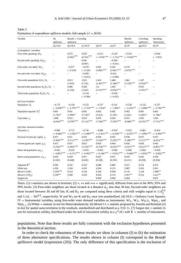
The results of the estimation of the different models are presented in Tables 2 and 3.presents the results of the estimation of different specifications with the full sample ofmunicipalities. The results of column (a) of Table 2 correspond to theNo-spilloversmodel (ex-pression (22)) and show that the different control variables introduced in the equation ato account for a sizeable proportion of local spending variation (roughly 50%). Moreover,of these variables are statistically significant and have the anticipated signs, with the proof young population being the sole exception to this rule. Local spending decreases anincreases with population. Local spending is higher as production costs increase, and ththe tax-price, the higher the personal income and transfers received, and the lower theold population. All these results are consistent with previous analyses of local spending in(Solé-Ollé [34]; and Bosch and Solé-Ollé [7]). However, it is unclear whether this is the apriate model, since the results of theMoran tests suggest that there is spatial correlation inerror terms, both with the first- and second-order neighbors’ matrices. This suggests a pomission of spatially correlated variables and the need to test whether some of our spmodels are appropriate.

The results of columns (b) to (e) correspond to theBenefit+ Crowding spilloversmodel. TheOLS results of column (b) suggest positive interactions between the spending of neighborinicipalities and a positive effect of first- and second-order neighbors’ populations, althoughlast two coefficients are not statistically significant. The effect of neighbors’ costs, contraryexpectations, is negative and not statistically significant. Things do not improve when sorder neighbors’ spending and costs and third-order populations are added (column (c)), mthat the problem does not seem to lie in the appropriate distance decay for these variablewe re-estimate by Instrumental Variables, the results greatly improve—see the resultsumn (d) and note that we still obtain statistically significant spending interactions, althousign is now negative. The results of the Sargan test at the bottom of the table suggestinstruments we have used in the estimation are valid.19 Moreover, the neighbors’ cost index nohas a positive and significant effect on spending, as suggested by our theoretical modresults of column (e) tell us that while second-order neighbors’ population does have anon spending, this is not true of second-order spending and costs, and of third-order nei

19 Given the high magnitude of the OLS bias implied by change in the sign of the interaction, we wonderedresults were driven by any of the instruments we used. To check this possibility we re-estimated by IV excludinstruments one-by-one and using a “differences-in-Sargan” statistic (Hayashi [24]) to test for the validity of eachment. This statistic has been computed as the difference of the Sargan statistics of the equations excluding andthe suspicious instrument, and is distributed as aχ2(K) with K = loss of over-identifying restrictions. All the instruments were valid and the results obtained when excluding one of them were not qualitatively different.


ndare

;

2]

.

esented

mation

on of

Table 2Estimation of expenditure spillover models: full sample (J = 2610)

Variable No

spillovers

Benefit+ Crowding

spillovers

Benefit

spillovers

Crowding

spillovers

Spending

interactions

(a) OLS (b) OLS (c) OLS (d) IV (e) IV (f) IV (g) OLS (h) IV

(i) Neighbors’ variables

First-order spending: Wei – 0.272 0.255 −0.213 −0.220 −0.224 – −0.064

(5.045)*** (4.741)*** (−2.918)∗∗∗ (−2.741)∗∗∗ (−3.018)∗∗∗ (−1.055)

Second-order spending: W2ei – – 0.041 – −0.046 – – –

(0.897) (−0.631)

First-order cost index: Wci – −0.077 −0.076 0.302 0.562 0.576 – –

(−0.354) (−0.320) (2.882)∗∗∗ (2.841)∗∗∗ (3.074)∗∗∗Second-order cost index: W2ci – – −0.000 – -0.032 – – –

(−0.013) (−0.069)

First-order population: KNi/Ni – 0.913 1.021 1.433 1.468 1.861 1.187 –

(1.632) (1.332) (2.407)∗∗∗ (2.369)∗∗ (3.150)∗∗∗ (2.054)∗∗Second-order population: K2Ni/Ni – 0.496 0.500 1.0 1.005 – 0.933 –

(1.532) (1.641) (3.147)∗∗∗ (3.056)∗∗∗ (2.501)∗∗Third-order population: K3Ni/Ni – – −0.154 – −0.058 – – –

(−0.368) (−0.621)

(ii) Cost variables

Population:Ni −0.175 −0.128 −0.125 −0.137 −0.141 −0.158 −0.132 −0.157

(−3.658)∗∗∗ (−2.707)∗∗∗ (−2.723)∗∗∗ (−1.914)∗ (−1.900)∗ (−2.214)∗∗ (−2.869)∗∗∗ (−2.706)∗∗∗Population squared:N2

i0.001 0.001 0.001 0.002 0.002 0.002 0.001 0.001

(1.745)∗ (1.899)∗ (1.745)∗ (1.621) (1.501) (1.431) (1.861)∗ (1.786)∗Cost index:ci 1.008 0.915 0.922 0.919 0.920 0.915 1.002 1.005

(6.618)∗∗∗ (5.078)∗∗∗ (5.112)∗∗∗ (7.506)∗∗∗ (7.435)∗∗∗ (6.948)∗∗∗ (6.555)∗∗∗ (7.113)∗∗∗

(iii) Voter demand variables

Tax-price:ti −0.885 −0.712 −0.736 −0.899 −0.910 −0.923 −0.801 −0.924

(−4.440)∗∗∗ (−3.392)∗∗∗ (−3.449)∗∗∗ (−6.361)∗∗∗ (−6.029)∗∗∗ (−6.655)∗∗∗ (−3.893)∗∗∗ (−4.269)∗∗∗Personal income per capita:yi 0.027 0.021 0.025 0.030 0.032 0.030 0.027 0.027

(5.439)∗∗∗ (5.111)∗∗∗ (5.239)∗∗∗ (5.529)∗∗∗ (5.505)∗∗∗ (5.489)∗∗∗ (5.517)∗∗∗ (4.023)∗∗∗Current grants per capita:gi ti 0.927 0.937 0.915 0.956 0.944 0.956 0.926 0.942

(5.516)∗∗∗ (5.495)∗∗∗ (5.333)∗∗∗ (6.754)∗∗∗ (6.632)∗∗∗ (5.637)∗∗∗ (5.617)∗∗∗ (4.967)∗∗∗Share old population:poi,t −0.061 −0.053 −0.055 −0.065 −0.066 −0.066 −0.062 −0.059

(−6.867)∗∗∗ (−6.117)∗∗∗ (−6.005)∗∗∗ (−9.144)∗∗∗ (−9.051)∗∗∗ (−9.046)∗∗∗ (−6.833)∗∗∗ (−6.002)∗∗∗Share young population:pyi,t 0.029 0.018 0.017 0.022 0.021 0.025 0.032 0.038

(0.345) (0.448) (0.465) (0.328) (0.305) (0.211) (0.258) (0.204)

AdjustedR2 0.502 0.522 0.519 0.488 0.485 0.471 0.514 0.475

White test 4.256 3.336 4.101 4.594 4.115 2.987 5.015 5.651

Moran’s I (W) 2.354∗∗∗ 0.214 0.124 0.320 0.284 0.110 1.224 1.984∗∗Moran’s I (W2) 2.100∗∗ 0.584 0.210 0.054 0.110 2.001∗∗ 0.214 2.412∗∗Sargan test – – – 0.000 0.000 0.004 – 0.021

Notes. (1) t -statistics are shown in brackets; (2)∗, ∗∗ and∗∗∗ = significantly different from zero at the 90%, 95% a99% levels. (3) First-order neighbors are those located at a distancedij less than 30 km; Second-order neighbors

those located between 30 and 60 km; K and K2 are computed using these criteria and with weights equal to 1/d0.5ij

and 1/(di − 30)0.5, respectively; W and W2 are K and K2 once row-standardized. (4) OLS= Ordinary Least SquaresIV = Instrumental variables, using first-order voter demand variables as instruments: Wτi , Wyi , Wgiτi , Wpoi,t andWpyi,t . (5) White= statistic to test for Heteroskedasticity. (6)Moran’s I = statistic proposed by Anselin and Kelejian [to test for spatial autocorrelation in the residuals, standardized and distributed as aN(0,1). (7) Sargan test= statistic totest for instrument validity, distributed under the null of instrument validity as aχ2(K) with K = number of instruments

populations. Note that these results are fully consistent with the exclusion hypotheses prin the theoretical section.

In order to check the robustness of these results we show in columns (f) to (h) the estiof three alternative specifications. The results shown in column (f) correspond to theBenefitspilloversmodel (expression (20)). The only difference of this specification is the exclusi


ptionct theferentcient

Table 3Benefit+ Crowdingspillovers:Urban vs.Non-UrbanandSuburbsvs.Centralcities

Variable Urban municipalities

(J = 1315)

Non-Urban municipalities

(J = 1295)

Suburbs

(J = 1259)

City centers

(J = 36)

(a) OLS (b) IV (c) OLS (d) IV (e) OLS (f) IV (g) OLS (h) IV

(i) Neighbors’ variables

First-order spending: Wei 0.491 −0.573 0.184 −0.151 0.540 −0.509 −0.046 −0.128

(8.756)∗∗∗ (−2.773)∗∗∗ (2.876)∗∗∗ (−1.899)∗ (9.100)∗∗∗ (−2.399)∗∗∗ (−0.044) (−0.839)

First-order cost index: Wci −0.183 0.712 0.158 0.125 −0.211 0.735 0.333 −0.284

(−0.545) (3.622)∗∗∗ (3.255)∗∗∗ (1.877)∗ (−0.613) (7.561)∗∗∗ (0.620) (−0.371)

First-order population: KNi/Ni 0.651 1.789 0.988 1.282 0.380 1.629 119.330 150.926

(1.900)∗ (2.877)∗∗∗ (1.853)∗ (2.023)∗∗ (1.436) (2.501)∗∗∗ (1.788)∗ (2.384)∗∗∗Second-order population: K2Ni/Ni 0.243 1.569 0.286 0.646 0.174 1.449 34.289 99.604

(0.735) (2.457)∗∗∗ (0.018) (1.564) (0.911) (2.143)∗∗∗ (2.631)∗∗∗ (1.794)∗

(ii) Cost variables

Population:Ni −0.203 −0.183 −0.759 −1.113 −0.478 −0.210 −0.031 −0.093

(−3.318)∗∗∗ (−1.935)∗ (−0.799) (−1.045) (−2.154)∗∗ (−1.887)∗ (−0.575) (−0520)

Population squared:N2i

0.002 0.002 0.001 0.001 0.002 0.002 0.000 0.001

(1.634) (1.512) (1.102) (0.951) (1.754)∗ (1.531) (0.241) (0.355)

Cost index:ci 1.179 1.059 0.878 0.892 1.168 1.397 1.022 1.181

(5.063)∗∗∗ (7.574)∗∗∗ (3.331)∗∗∗ (6.160)∗∗∗ (4.995)∗∗∗ (3.398)∗∗∗ (1.938)∗ (1.707)∗

(iii) Voter demand variables

Tax-price:τi −1.114 −1.113 −0.485 −0.674 −1.110 −1.115 −0.951 −0.874

(−3.189)∗∗∗ (−5.103)∗∗∗ (−1.748)∗ (−3.376)∗∗∗ (−3.178)∗∗∗ (−5.148)∗∗∗ (−2.114)∗∗ (−1.874)∗Personal income per capita:yi 0.014 0.034 0.024 0.031 0.013 0.033 0.015 0.047

(6.001)∗∗∗ (7.787)∗∗∗ (7.709)∗∗∗ (8.239)∗∗∗ (5.398)∗∗∗ (7.304)∗∗∗ (2.996)∗∗∗ (2.369)∗∗Current grants per capita:gi ti 0.792 0.978 0.957 0.912 0.794 0.984 0.785 0.954

(5.189)∗∗∗ (5.117)∗∗∗ (6.075)∗∗∗ (4.168)∗∗∗ (5.207)∗∗∗ (5.611)∗∗∗ (1.987)∗∗ (2.183)∗∗Share old population:poi,t −0.064 −0.114 −0.043 −0.048 −0.065 −0.111 −0.045 −0.033

(−5.963)∗∗∗ (−7.901)∗∗∗ (−3.046)∗∗∗ (−4.845)∗∗∗ (−5.961)∗∗∗ (−5.966)∗∗∗ (−1.422) (−1.365)

Share young population:pyi,t 0.023 0.048 0.063 0.026 0.025 0.048 0.020 0.094

(0.177) (0.268) (0.257) (1.142) (0.244) (0.256) (0.371) (0.522)

AdjustedR2 0.572 0.483 0.508 0.473 0.595 0.563 0.480 0.364

White test 5.541 5.510 4.580 4.261 5.688 5.981 5.677 5.559

Moran’s I (W) 0.412 0.335 0.455 0.235 0.745 0.555 0.449 0.620

Moran’s I (W2) 0.175 0.058 0.201 0.559 0.659 0.108 0.016 0.077

Sargan test – 0.001 – 0.000 – 0.002 – 0.000

Note. (1) See Table 2.

Table 4EstimatedBenefitandCrowdingspillovers parameters

Samples Benefitspillovers Crowdingexternalities

θ z-value δ z-value

Full sample 0.329 (4.121)∗∗∗ 0.059 (2.632)∗∗∗Urbanmunicipalities 0.675 (4.309)∗∗∗ 0.242 (2.131)∗∗Non-Urbanmunicipalities 0.141 (1.601) 0.042 (1.578)Suburbs 0.690 (3.128)∗∗∗ 0.273 (2.671)∗∗∗City centers 0 (0.551) 0.461 (1.801)∗

Notes. (1) θ computed using expression (23);δ computed using expression (24) for all the samples to the exceof City centers; for City centers, δ computed using expression (26). (2) The derivatives of spending with respedifferent variables used to computeθ andδ use sample-specific values for the estimated coefficients and for the difvariables involved. (3)z-valuesdistributed as aN(0,1) and computed as the ratio between the value of the coeffiand its standard error; standard errors computed using the formula for the variance of provided in Rao [31]. (4)∗, ∗∗ and∗∗∗ = significantly different from zero at the 90%, 95% and 99% levels.


The IVof thettle bitcludedln (d))of the

ificantexcludesoreticalarisonsed inand goticallyficientat therefore,

that the

ding ofeck therelativesign ofcond,model

tingenting the

ing inr times

f theseheyent as

pter (vi)l

the second-order neighbor’s populations. The OLS results are omitted to save space.results are similar to the previous ones (see column (d)), with the relevant coefficientssame sign and magnitude. However, the explanatory capacity of the model drops a liand thet-statistic clearly suggests that second-order neighbor’s populations cannot be exfrom the equation. The results in column (h) correspond to theCrowdingexternalities mode(expression (21)). The only differences between this specification and the full model (columis the exclusion of neighbor’s spending and costs. The results are quite similar to thosefull model, with first- and second-order neighbor’s populations having a positive and signimpact on spending. However, the results suggest that also in this case is not possible toneighbor’s spending and costs. Finally, column (h) shows the results of theSpending Interactionmodel. This specification does not correspond to any of the equations developed in the thesection. However, we have decided to show the results of this equation to allow the compof its performance with the other equations estimated, given that this is the specification uprevious studies (e.g., Case et al. [15] and Baicker [4]). We also omit here the OLS resultsdirectly to the IV ones, that show that the neighbor’s spending coefficient is no longer statissignificant, while the OLS results (not included here) showed a positive and significant coef(as in the other OLS results with neighbor’s spending included in Table 2). Note also thMoran’s I statistic suggest both first- and second-order residual spatial correlation. Thewe should conclude that theSpending Interactionsmodel is not the appropriate one.

The check on exclusion constraints presented in the previous section thus suggestscorrect model for including the effects of spillovers is theBenefit+ Crowding spilloversmodel,which accounts simultaneously for spending interactions and for the effects on local spenfirst-order neighbors’ costs and first- and second-order neighbors’ populations. We can chrobustness of the results by analyzing the additional hypothesis regarding the sign and thesize of the coefficients developed in the previous section. First, note that, as expected, thethe neighbors’ spending is negative while that of the neighbors’ cost index is positive. Sethe effect of the own cost variable is much higher than the effect of neighbors’ costs, as thesuggested. Moreover, we could use expression (28) to compute the derivatives ofEi with respectto first- and second-order neighbor’s population. Since these derivatives are, however, conon the distance, we compute them at different distances (i.e, 1, 7.5, 15 and 30 km) usmean sample values of the different variables involved.20 The values we get for∂Ei/∂Nj are20.38 (1 km), 7.44 (7.5 km), 5.26 (15 km) and 3.72 (30 km) and the value we get for∂Ei/∂Nl

at 30 km is 1.016. Note that by construction, the effect of first-order population is decreasdistance. In any case, however, the effect of first-order population at 30 km is three to fouthe effect of second-order population at this distance.

Finally, we can use expressions (23) and (24) to compute theBenefitandCrowding spilloversparameters, respectively. In this case, these parameters take the values ofθ = 0.33 andδ = 0.059and are statistically significant at the 95% level (see Table 4 for a summary of the values oparameters for different samples).21 Spillovers therefore not only seem to be relevant, but tare also sizeable. One Euro of local spending provides the same utility to a typical resid

20 The values used for the parameters of expression (28) are:α1 = 0.213 (see Table 2),β = 1/7.82 (with an averagedistance between municipalities of 10.1 km and an average number of 36 neighbors per municipality),ej = 326 (seeTable 1),Ni/Nj = 2,134,α4 = 1.433 andα5 = 1.016.21 Standard errors have been computed using the formula for the variance provided in Theorem (ii) of Chaof Rao [31], which can be expressed ass2

E= ∑

i νij (∂χ/∂ai )(∂χ/∂aj ), whereχ ≡ (θ, δ) is the vector of structuraparameters anda ≡ (∂E/∂c, ∂E/∂c+1, ∂E/∂N,∂E+1/∂N+2) is the vector of estimated coefficients.


ads toditional

odailyan ar-

-

i-. Itesalso

n the

m a cityedure,

w

ee Ta-ntshighersince5%

9 for theutificantbors’found

ional

fullr

derssarilyay bes

three Euro of neighbors’ spending, and an additional non-resident living 30 km away lethe quality of public services in the locality decreasing less than ten times less than an adresident would.

Table 3 presents the results obtained when breaking the sample intoUrban andNon-Urbanmunicipalities, and when considering theSuburbsand theCity centersseparately. There are twintuitions behind this analysis. The first intuition is that if spillovers arise because of themobility of citizens between municipalities, they should be more pronounced in large urbeas, where mobility is also more relevant. The second intuition is that in urban areas,Benefitspilloversmay be more prevalent in theSuburbs,andCrowding externalitiess may be more important inCity centers. This is becauseCity centersare much bigger thanSuburbsand play aprominent role as employment and administrative centers.City centerstherefore usually experence a net inflow of population whileSuburbsusually experience (on average) a net outflowis therefore to be expected that residents in theSuburbstend to benefit more from the servicprovided in other localities thanCity centerresidents and, at the same time, we can expectthat the services in theCity centersare more crowded by non-residents than the services iSuburbs.

To test these hypotheses, we divided our sample intoUrbanandNon-Urbanareas. In line withprevious analyses, urban municipalities were defined as those located less than 35 km frocenter with more than 100,000 inhabitants (Solé-Ollé and Viladecans [35]). Using this procwe are able to identify 36 large urban areas that contain 1259Suburbsand 36City centers. Wetherefore have 1315Non-Urbanand 1295Urban municipalities. The results of Table 3 shoimportant differences betweenUrban andNon-Urbanmunicipalities. The results for theUrbanmunicipalities (columns (a) and (b)) are similar to those presented for the full sample (sble 2), since bothBenefitandCrowdingspillovers matter. However, the size of the coefficiefor the neighbor’s variables is now bigger than before, suggesting that spillovers are of amagnitude. This intuition is confirmed by the identification of the two spillover parameters,we found thatθ = 0.67 andδ = 0.24. These coefficients are statistically significant at the 9level (see Table 4). It should be remembered that these parameters were 0.33 and 0.05full sample. The results for theNon-Urbanmunicipalities (columns (c) and (d)) are similar, bthe size of the neighbors’ coefficients is lower and some of them are not statistically sign(second-order population) or only statistically significant at the 90% level (first-order neighspending and costs). The value of the spillover coefficients is now much lower, since wethatθ = 0.14 andδ = 0.04, but these coefficients are not statistically significant at conventlevels (see Table 4). We can conclude, therefore, that spillovers are more relevant inUrban thanin Non-Urbanareas, as expected.

The results of Table 3 also show significant important differences betweenSuburbsandCitycenters. The results for theSuburbs(columns (e) and (f)) are virtually the same as for thesample ofUrban municipalities. The results for theCity centersare different. Both first-ordeneighbors’ spending and costs are not statistically significant, suggesting thatBenefit spilloversare not present, and that onlyCrowding externalitiesare relevant. The fact that second-orneighbors’ populations have a positive and statistically significant effect does not nececontradict this statement, since it may simply mean that the distance decay function mdifferent forCity centersthan forSuburbs. The identification of spillover coefficients confirmthese conclusions. For theSuburbs, we found thatθ = 0.69 andδ = 0.27 while forCity centers,


veleresultslved

lovers,

t types

ne ofvers areers are

Thesegnitude,

with

funda-nditure

models.also beoweverypothe-

acceptnce ofclusiont vari-tion ofments,s (e.g.,

by theeal withlover’suse of, in anyeen thedencective,a lower

we found thatθ = 0 andδ = 0.46.22 The coefficients are statistically significant at the 95% lefor Suburbsbut in the case ofCity centersonly theδ coefficient is statistically significant at th90% (see Table 4). These results confirm our expectations. We admit, however, that thefor City centersshould be taken with caution, given the small number of observations invoand the lower explanatory power of the expenditure equation.

4. Conclusion

The simple model sketched in this paper allowed us to test for the presence of spilconfirming that this is a relevant problem in Spain, and that this problem is more acute inUrbanareas than in the rest of the country. The model allowed us to differentiate between differenof spillovers. We showed that two different kinds of spillovers (Benefit spilloversandCrowdingexternalities) should be taken into account in this kind of analysis. Failure to account for othese types of spillovers leads false inferences being drawn, suggesting either that spillopresent when they are not or that they are not relevant when they are. Both kinds of spillovimportant in theSuburbsbut only one type (Crowding externalities) is relevant inCity centers.The model also allowed us to obtain an estimate of the size of each type of spillovers.results suggest that spillovers are not only present but also are of a considerable maespecially inUrban areas. The magnitude of the inefficiencies (and inequities) associatedthese spillovers should therefore be a concern for policy-makers.

However, we have to admit that the approach used in the paper may have at least twomental weakness that merit some further comments. First, it can be argued that the expeinteractions generated by the model may also arise as a result of alternative behavioralFor example, as Brueckner [12] points out, interactions between local governments maypredicted by the standard tax competition model (Brueckner and Saavedra [13]). Note hthat, although the model has not been designed to provide a test against other competing hses, it provides a set of predictions that must be fulfilled by the empirical results in order tothe spillover story is plausible. These hypotheses refer not only to the statistical significaspatially lagged expenditure, as in previous analyses (Case et al. [15]), but also to the inof other neighbors’ covariates, and to the sign and size of the coefficients of the differenables. Moreover, household fiscal mobility is not seen as a tight constraint on the operalocal governments in Spain. This is the result of the limited scope of Spanish local governwhich do not provide the services that cause the mobility experienced in other countrieeducation in the US).

Second, one may wonder to what extent the fiscal interactions identified are drivenoperation of matching grants, user charges, or any other fiscal instruments designed to dthe externalities, instead of being the result of the reaction of local governments to the spilproblem. But as we have argued in Section 4.2, Spanish local governments make littlemost of the instruments that use to be recommended to internalize these externalities. Andcase, if these instruments where used effectively we should observe no interactions betwfiscal choices of neighboring municipalities. Note that, instead of this, we have found eviof sizeable spillovers. If externality-correcting instruments were present but not fully effethen the estimated magnitude of the spillovers obtained in the paper should be consideredbound of its real value.

22 Given thatθ = 0, in this case we made use of expression (26) to identifyδ, using the expression∂Ei/∂Ni = (α2Ni −2α3N2

i) + ei .


hesisd in this

national

(1981)

onomic

onomic

Lessons

rnal of

litical

mics 33

ational

urnal of

nce and

e states,

Urban

nance 3

) 437–

of Eco-

) 567–

ngton,

Eco-

sis and

toregres-–121.pkins

31–547.

Therefore, although we acknowledge that further efforts to explicitly test our hypotagainst competing ones are necessary, we therefore consider that the results providepaper show some preliminary evidence in favor of our model.

References

[1] L. Anselin, Spatial Econometrics, Methods and Models, Kluwer Academic, Dordrecht, 1988.[2] L. Anselin, H. Kelejian, Testing for spatial autocorrelation in the presence of endogenous regressors, Inter

Regional Science Review 20 (1999) 153–182.[3] R. Arnott, R.E. Grieson, Optimal fiscal policy for a state or local government, Journal of Urban Economics 9

23–48.[4] K. Baicker, The spillover effects of state spending, Journal of Public Economics 89 (2–3) (2005) 529–544.[5] T. Besley, A. Case, Incumbent behaviour, vote-seeking, tax setting and yardstick competition, American Ec

Review 85 (1995) 25–45.[6] T.E. Borcherding, R.T. Deacon, The demand for the services of non federal governments, American Ec

Review 62 (1972) 891–901.[7] N. Bosch, A. Solé-Ollé, On the relationship between authority size and the costs of providing local services:

for the design of intergovernmental transfers in Spain, Public Finance Review 33 (2005) 318–342.[8] M.J. Boskin, Local government tax and product competition and the optimal provision of public goods, Jou

Political Economy (1973) 203–210.[9] W. Brainard, F.T. Dolbear, The possibility of oversupply of local ‘public’ goods, a critical note, Journal of Po

Economy 75 (1967) 86–90.[10] G. Bramley, Equalization Grants and Local Expenditure Needs, Avebury, England, 1990.[11] C. Brett, J. Pinkse, The determinants of municipal tax rates in British Columbia, Canadian Journal of Econo

(2000) 695–714.[12] J.K. Brueckner, Strategic interactions among governments; an overview of the empirical literature, Intern

Regional Science Review 26 (2) (2003) 175–188.[13] J.K. Brueckner, L.A. Saavedra, Do local governments engage in strategic property tax competition? Jo

Urban Economics 54 (2001) 203–229.[14] T. Buettner, Local business taxation and competition for capital, the choice of the tax rate, Regional Scie

Urban Economics 31 (2–3) (2001) 215–245.[15] A.C. Case, J.R. Hines, H.S. Rosen, Budget spillovers and fiscal policy interdependence, evidence from th

Journal of Public Economics 52 (1993) 285–307.[16] J. Conley, M. Dix, Optimal and equilibrium membership in clubs with the presence of spillovers, Journal of

Economics 46 (1999) 215–229.[17] B. Dalhby, Fiscal externalities and the design of intergovernmental grants, International Tax and Public Fi

(1994) 397–412.[18] D.N. Figlio, V.W. Kolpin, W.E. Reid, Do states play welfare games? Journal of Urban Economics 46 (1999

454.[19] W.S. Furlog, S.L. Mehay, Urban law enforcement in Canada, an empirical analysis, Canadian Journal

nomics 14 (1981) 44–57.[20] R.H. Gordon, An optimal taxation approach to fiscal federalism, Quarterly Journal of Economics 98 (1983

586.[21] K.V. Greene, W.B. Neenan, C.D. Scott, Fiscal Interactions in a Metropolitan Area, Lexington Books, Lexi

1977.[22] S.A. Hakim, E.S. Ovadia, J. Weinblatt, Interjurisdictional spillovers of crime and police expenditure, Land

nomics 55 (1979) 200–212.[23] A.K. Haughwout, Regional fiscal cooperation in metropolitan areas, an exploration, Journal of Policy Analy

Management 18 (1999) 579–600.[24] F. Hayashi, Econometrics, first ed., Princeton Univ. Press, Princeton, NJ, 2000.[25] H.H. Kelejian, I. Prucha, A generalised spatial two-stage lest squares procedure for estimating a spatial au

sive model with autoregressive disturbances, Journal of Real Estate Finance and Economics 17 (1998) 99[26] H.F. Ladd, J. Yinger, American Ailing Cities, Fiscal Health and the Design of Urban Policy, The Johns Ho

Univ. Press, Baltimore/London, 1989.[27] J. Le Grand, Fiscal equity and central government grants to local authorities, Economic Journal 85 (1975) 5


ditures,

olitical

2000)

conomía

egional

7) 557–

.), The

[28] J. Murdoch, M. Rahmatian, M. Thayer, A spatially autoregressive median voter model of recreation expenPublic Finance Quarterly 21 (1993) 334–350.

[29] W.E. Oates, Fiscal Federalism, Harcourt Brace Jovanovich, New York, 1972.[30] M. Pauly, Optimality, ‘public’ goods and local governments, a general theoretical analysis, Journal of P

Economy 78 (1970) 572–585.[31] C.R. Rao, Linear Statistical Inference and Its Applications, Wiley, New York, 1965.[32] J. Rothenberg, Poverty and urban public expenditures, Urban Studies 35 (1998) 1995–2019.[33] L.A. Saavedra, A model of welfare competition with evidence from AFDC, Journal of Urban Economics 47 (

248–279.[34] A. Solé-Ollé, Determinantes del gasto público local: Necesidades de gasto o capacidad fiscal? Revista de E

Aplicada 25 (2001) 115–156.[35] A. Solé-Ollé, E. Viladecans-Marsal, Central cities as engines of metropolitan area growth, Journal of R

Science 44 (2) (2004) 321–350.[36] D. Staiger, J.H. Stock, Instrumental variable regression with weak instruments, Econometrica 5 (65) (199

586.[37] B.A. Weisbrod, Geographic spillover effects and the allocation of resources to education, in: J. Margolis (Ed

Public Economy of Urban Communities, Resources for the Future, Washington, DC, 1965, pp. 33–50.

expenditure spillovers and ﬁscal interactions: empirical

Documents