ecuaciones diferenciales de primer orden. caída libre con ... · caída libre con resistencia del...
TRANSCRIPT
Ecuaciones Diferenciales de Primer
Orden. Caída Libre con Resistencia
del Aire.
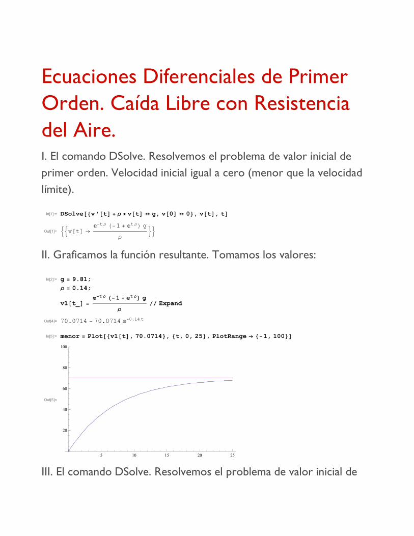
I. El comando DSolve. Resolvemos el problema de valor inicial de
primer orden. Velocidad inicial igual a cero (menor que la velocidad
límite).
In[1]:= DSolve@8v'@tD + Ρ * v@tD � g, v@0D � 0<, v@tD, tD
Out[1]= ::v@tD ®ã-t Ρ H-1 + ãt ΡL g
Ρ
>>
II. Graficamos la función resultante. Tomamos los valores:
In[2]:= g = 9.81;
Ρ = 0.14;
v1@t_D =ã-t Ρ H-1 + ãt ΡL g
�� Expand
Out[4]= 70.0714 - 70.0714 ã-0.14 t
In[5]:= menor = Plot@8v1@tD, 70.0714<, 8t, 0, 25<, PlotRange ® 8-1, 100<D
Out[5]=
5 10 15 20 25
20
40
60
80
100
III. El comando DSolve. Resolvemos el problema de valor inicial de
primer orden. Velocidad inicial mayor que la velocidad límite.

III. El comando DSolve. Resolvemos el problema de valor inicial de
primer orden. Velocidad inicial mayor que la velocidad límite.
In[6]:= Clear@v, tDDSolve@8v'@tD + Ρ * v@tD � g, v@0D � 90<, v@tD, tD
Out[7]= 99v@tD ® 70.0714 ã-0.14 t I0.284404 + 1. ã
0.14 tM==
IV. Graficamos la función resultante. Tomamos los valores:
In[8]:= v2@t_D = 70.0714 ã-0.14 t I0.284404 + ã
0.14 tM �� Expand
Out[8]= 70.0714 + 19.9286 ã-0.14 t
In[9]:= mayor = Plot@8v2@tD, 70.0714<, 8t, 0, 25<, PlotRange ® 8-1, 100<D
Out[9]=
5 10 15 20 25
20
40
60
80
100
V. Ambas gráficas:
In[10]:= Show@menor, mayorD
Out[10]=
5 10 15 20 25
20
40
60
80
100
2 Caida_Resistencia_Aire.nb

VI. El campo de direcciones asociado a la ED.
In[12]:= campo = VectorPlot@81, g - Ρ * v<, 8t, 0, 60<, 8v, 0, 80<, AspectRatio ® AutomaticD
Out[12]=
0 10 20 30 40 50 60
0
20
40
60
80
In[14]:= Show@menor, mayor, campoD
Out[14]=
5 10 15 20 25
20
40
60
80
100
Caida_Resistencia_Aire.nb 3

VII. ¿Qué es la solución general de una ED?
In[15]:= DSolve@v'@tD + Ρ * v@tD � g, v@tD, tD
Out[15]= 99v@tD ® 70.0714 + ã-0.14 t
C@1D==
In[27]:= familia = PlotAEvaluateATableA970.0714 + C * ã-0.14*t
, 70.0714=, 8C, -100, -70<EE,
8t, 0, 25<, PlotRange ® 8-1, 80<E
Out[27]=
5 10 15 20 25
20
40
60
80
VIII. ¿Qué es una solución particular de una ED?
In[64]:= datoinicial = ListPlot@885, 25.2<<, PlotStyle ® 8Red, [email protected]<D
Out[64]=
2 4 6 8 10
10
20
30
40
50
4 Caida_Resistencia_Aire.nb
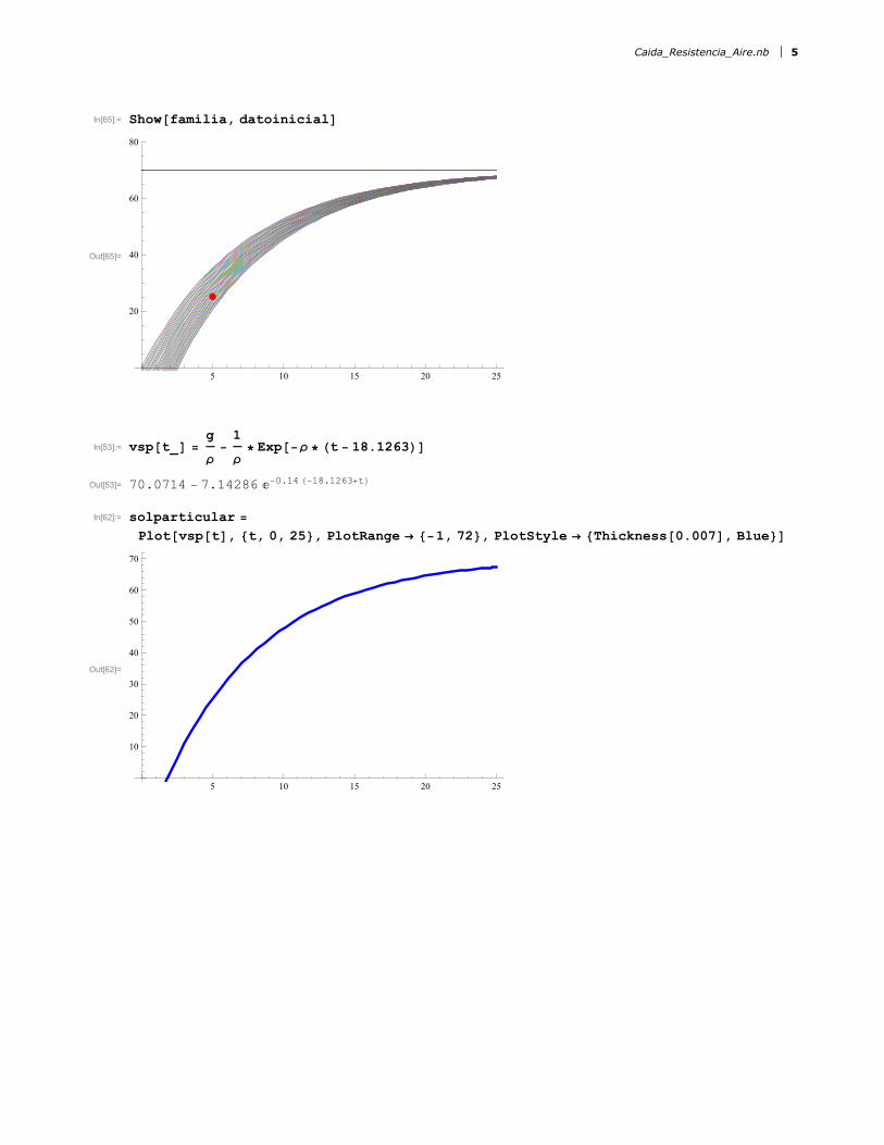
In[65]:= Show@familia, datoinicialD
Out[65]=
5 10 15 20 25
20
40
60
80
In[53]:= vsp@t_D =g
Ρ-
1
Ρ* Exp@-Ρ * Ht - 18.1263LD
Out[53]= 70.0714 - 7.14286 ã-0.14 H-18.1263+tL
In[62]:= solparticular =
Plot@vsp@tD, 8t, 0, 25<, PlotRange ® 8-1, 72<, PlotStyle ® [email protected], Blue<D
Out[62]=
5 10 15 20 25
10
20
30
40
50
60
70
Caida_Resistencia_Aire.nb 5

In[67]:= Show@familia, solparticular, datoinicialD
Out[67]=
5 10 15 20 25
20
40
60
80
6 Caida_Resistencia_Aire.nb