¿de qué estamos hechos? -...
TRANSCRIPT
¿De qué estamos hechos?Partículas e interacciones elementales
Carlos Pena
Física de Partículas Elementales y Cosmología
CRIF Acacias, Febrero 2012
Plan
Introducción: escalas de espacio y de energía en Física Fundamental.
Física Cuántica y Relatividad Especial.
Las preguntas revolucionarias.
Dirac y la Mecánica Cuántica Relativista.
Las interacciones nucleares débil y fuerte: neutrinos y mesones.
Interludio: diagramas de Feynman.
Teoría Cuántica de Campos.
Efectos cuánticos y fuerzas fundamentales.
Infinitos y Guerras.
La Edad de Plata: Electrodinámica Cuántica y leyes fundamentales.
Simetrías: la Edad de Oro.
El Camino Óctuple: Quarks.
La interacción electrodébil: corrientes neutras.
Más infinitos.
El Modelo Estándar de la Física de Partículas.

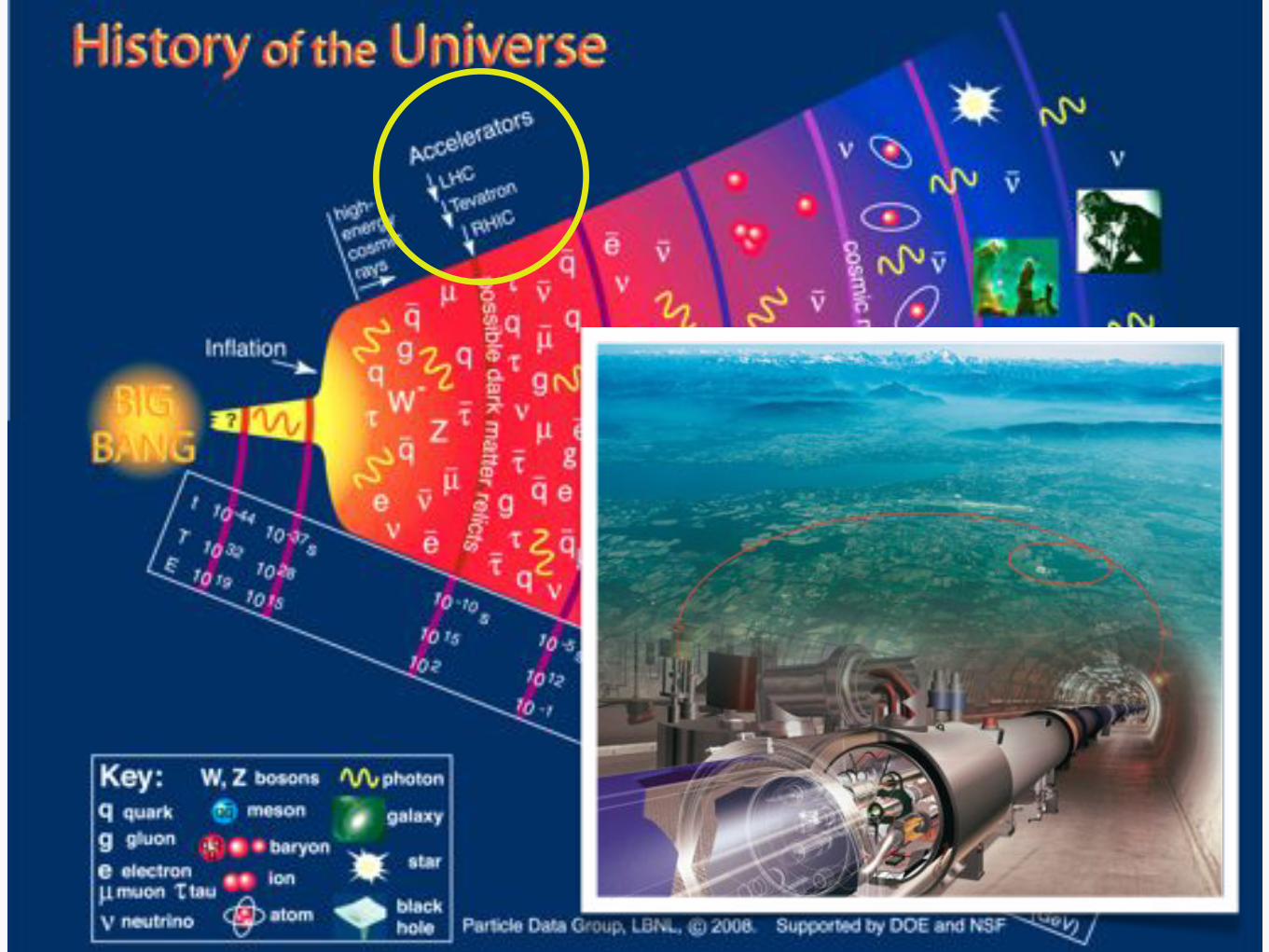
El sentido de la pregunta: escalas de longitud
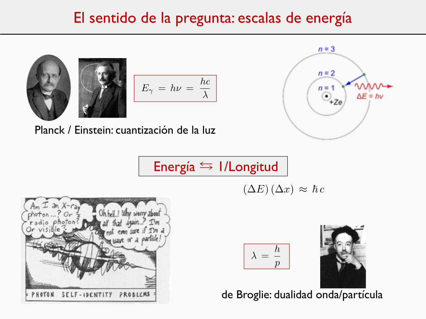
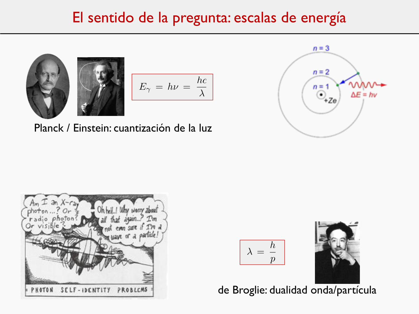
El sentido de la pregunta: escalas de energía
Planck / Einstein: cuantización de la luz
Eγ = hν =hc
λ
de Broglie: dualidad onda/partícula
λ =h
p
Energía ⇆ 1/Longitud
(∆E) (∆x) ≈ � c
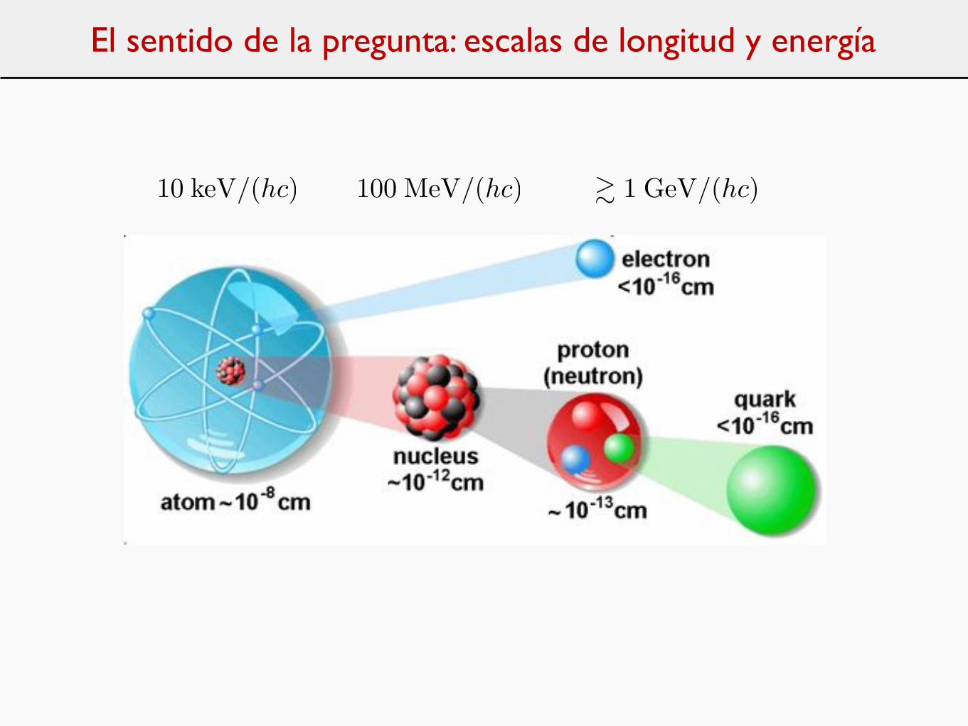
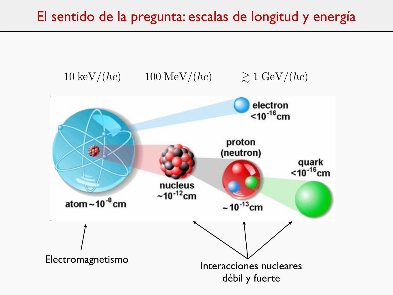
El sentido de la pregunta: escalas de longitud y energía
10 keV/(hc) 100 MeV/(hc) � 1 GeV/(hc)

ElectromagnetismoInteracciones nucleares
débil y fuerte
El sentido de la pregunta: escalas de longitud y energía
10 keV/(hc) 100 MeV/(hc) � 1 GeV/(hc)
El sentido de la pregunta: escalas de energía
Planck / Einstein: cuantización de la luz
Eγ = hν =hc
λ
de Broglie: dualidad onda/partícula
λ =h
p

ElectromagnetismoInteracciones nucleares
débil y fuerte
El sentido de la pregunta: escalas de longitud y energía
10 keV/(hc) 100 MeV/(hc) � 1 GeV/(hc)
19001910
1920
1930
1940
1950
1960
1970
1980
19902000
2010
CamposPartículasElectromagnético
Relatividad especial
Mecánica CuánticaOnda / partícula
Fermiones / Bosones
Dirac Antimateria
Bosones W
QED
Maxwell
Higgs
Supercuerdas?
Universo
NewtonMecánica Clásica,Teoría Cinética,Thermodinámica
MovimientoBrowniano
Relatividad General
Nucleosíntesis cosmológica
Inflación
Átomo
Núcleo
e-
p+
n
Zoo de partículas
u
µ -
!
"e
"µ
"!
d s
c
!-
!-
b
t
Galaxias ; Universo en expansión;
modelo del Big Bang
Fusión nuclear
Fondo de radiación de microondas
Masas de neutrinos
ColorQCD
Energía oscura
Materia oscura
W Zg
Fotón
Débil Fuerte
e+
p-
Desintegración betai Mesones
de Yukawa
Boltzmann
Radio-actividad
Tecnología
Geiger
Cámara de niebla
Cámara de burbujase
Ciclotrón
Detectores Aceleradores
Rayos cósmicos
Sincrotrón
Aceleradores e+e
Aceleradoresp+p-
Enfriamiento de haces
Online computers
WWW
GRID
Detectores modernos
Violación de P, C, CP
MODELO ESTÁNDAR
Unificación electrodébil
3 familias
Inhomgeneidades del fondo de microondas
1895
1905
Supersimetría?
Gran unificaci’on?
Cámara de hilos
Plan
Introducción: escalas de espacio y de energía en Física Fundamental.
Física Cuántica y Relatividad Especial.
Las preguntas revolucionarias.
Dirac y la Mecánica Cuántica Relativista.
Las interacciones nucleares débil y fuerte: neutrinos y mesones.
Interludio: diagramas de Feynman.
Teoría Cuántica de Campos.
Efectos cuánticos y fuerzas fundamentales.
Infinitos y Guerras.
La Edad de Plata: Electrodinámica Cuántica y leyes fundamentales.
Simetrías: la Edad de Oro.
El Camino Óctuple: Quarks.
La interacción electrodébil: corrientes neutras.
Más infinitos.
El Modelo Estándar de la Física de Partículas.
Mecánica Cuántica y Relatividad Especial
Las revoluciones cuántica y relativista se desarrollan en paralelo durante 30 años.
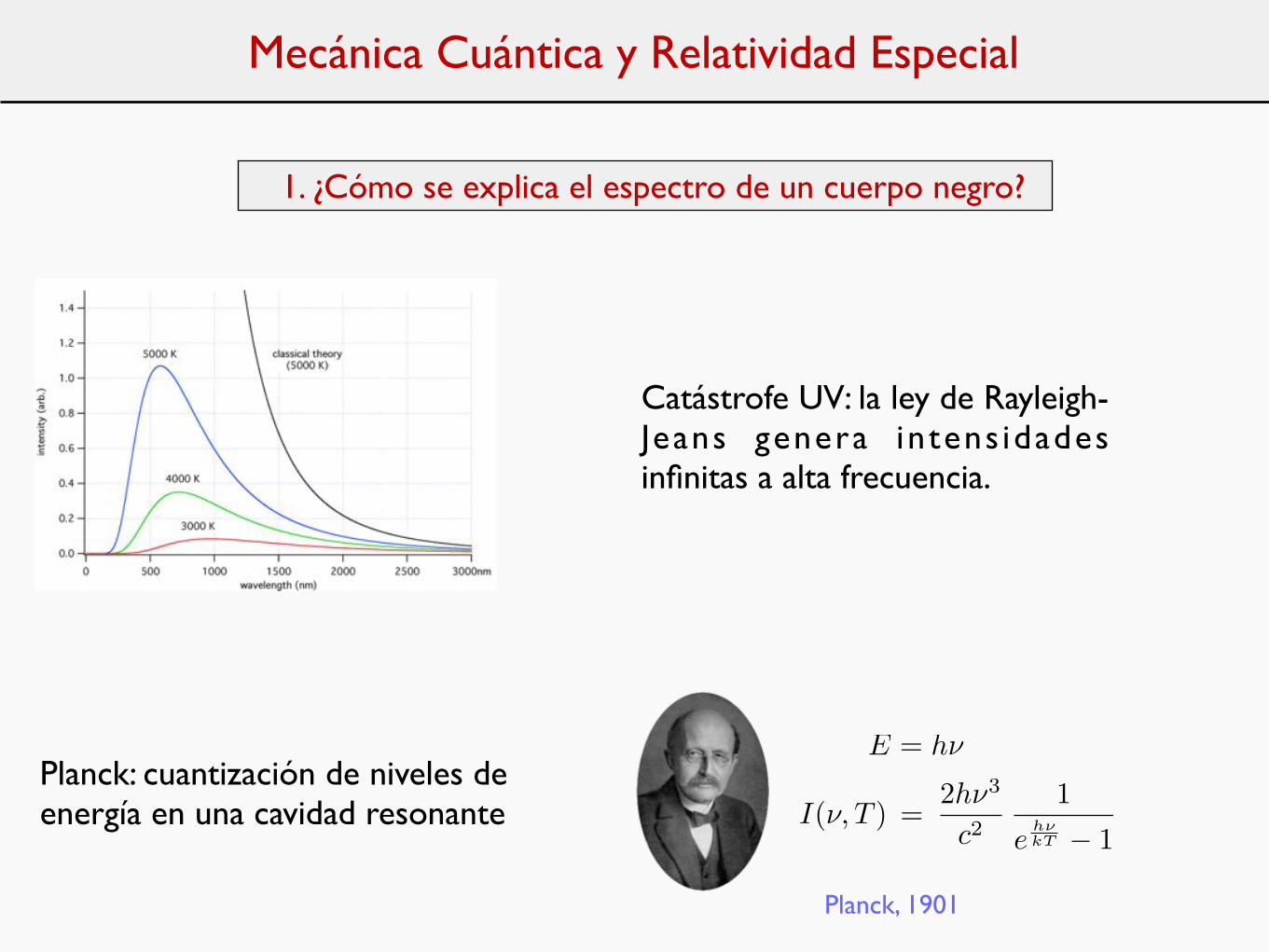
Planck: cuantización de niveles de energía en una cavidad resonante
Catástrofe UV: la ley de Rayleigh-Jeans genera intens idades infinitas a alta frecuencia.
1. ¿Cómo se explica el espectro de un cuerpo negro?
Planck, 1901
I(ν, T ) =2hν3
c2
1e
hνkT − 1
E = hν
Mecánica Cuántica y Relatividad Especial
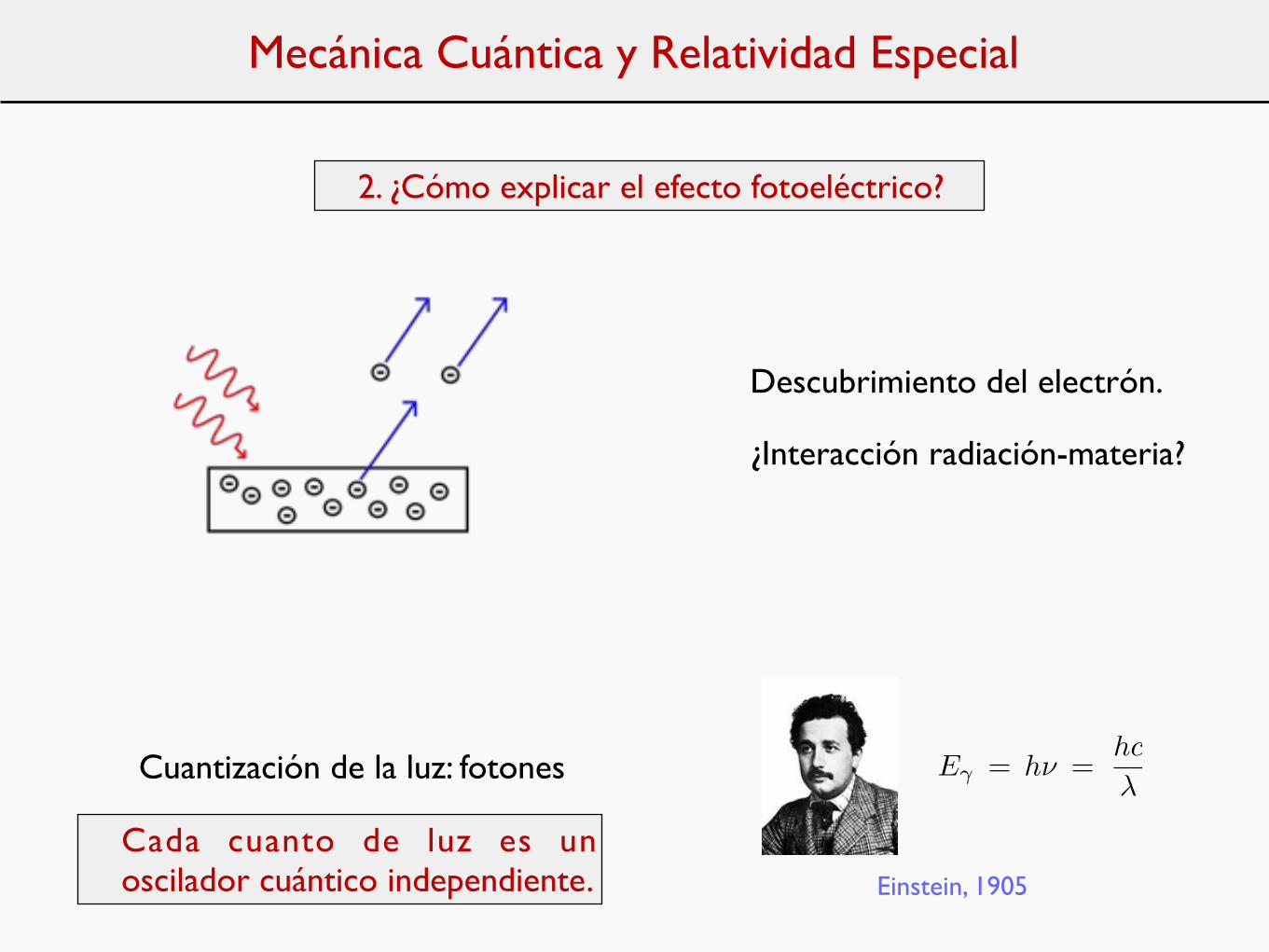
2. ¿Cómo explicar el efecto fotoeléctrico?
Einstein, 1905
Descubrimiento del electrón.
¿Interacción radiación-materia?
Cuantización de la luz: fotones
Cada cuanto de luz es un oscilador cuántico independiente.
Eγ = hν =hc
λ
Mecánica Cuántica y Relatividad Especial
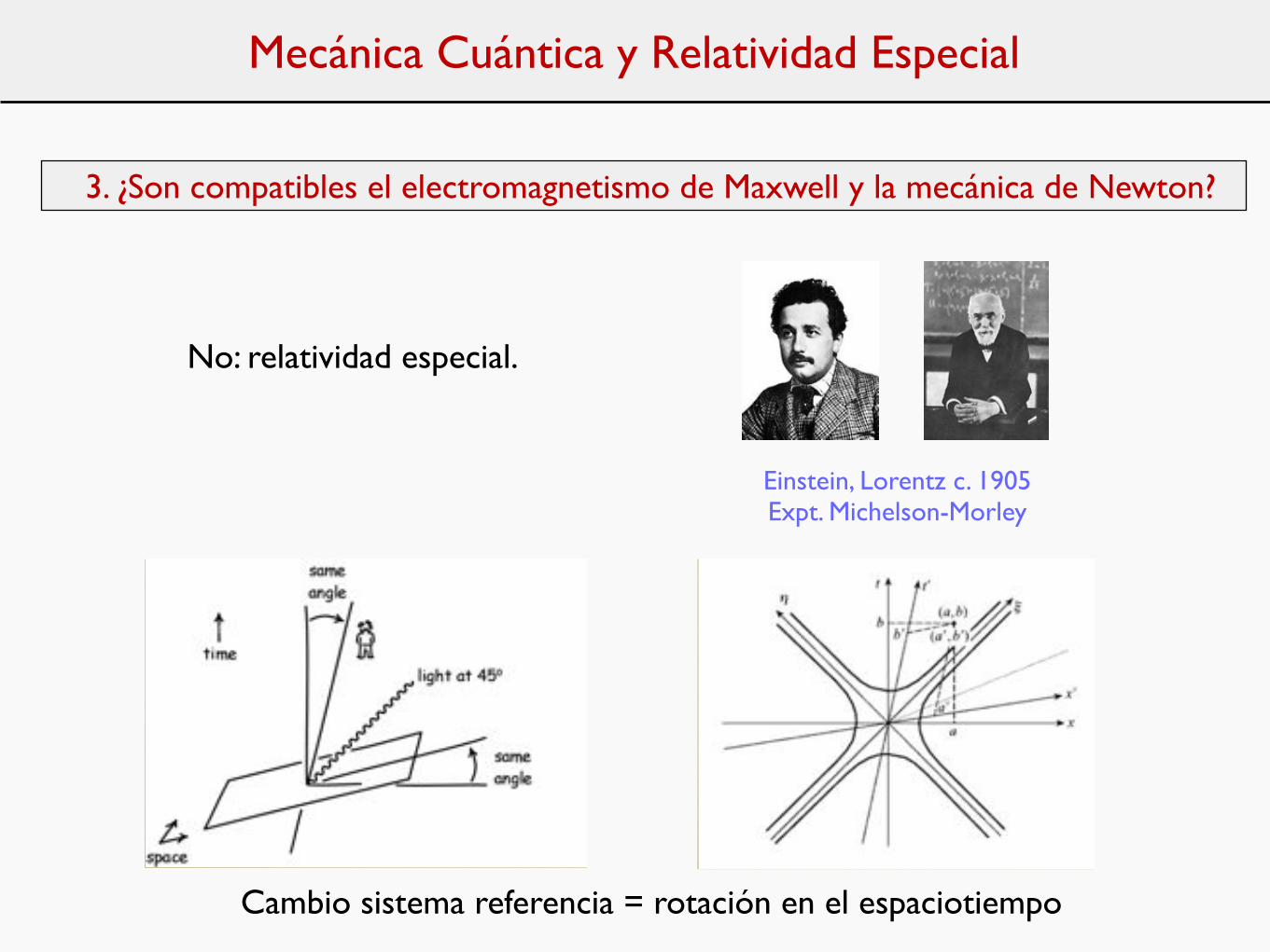
3. ¿Son compatibles el electromagnetismo de Maxwell y la mecánica de Newton?
No: relatividad especial.
Einstein, Lorentz c. 1905Expt. Michelson-Morley
Relatividad Especial
Espacio-Tiempo
1908
H. Minkowski
El espacio en sí y el tiempo en sí están abocados a desaparecer, y sólo una unión de ambos se mantendrá como una realidad independiente.Space by itself and time by itself, are doomed to fade away into mere shadows, and only a kind of union of the two will preserve an independent reality.
Cambio de sistema referencial como ‘rotación en el espaciotiempo’
Relatividad Especial
Espacio-Tiempo
1908
H. Minkowski
El espacio en sí y el tiempo en sí están abocados a desaparecer, y sólo una unión de ambos se mantendrá como una realidad independiente.Space by itself and time by itself, are doomed to fade away into mere shadows, and only a kind of union of the two will preserve an independent reality.
Cambio de sistema referencial como ‘rotación en el espaciotiempo’Cambio sistema referencia = rotación en el espaciotiempo
Mecánica Cuántica y Relatividad Especial
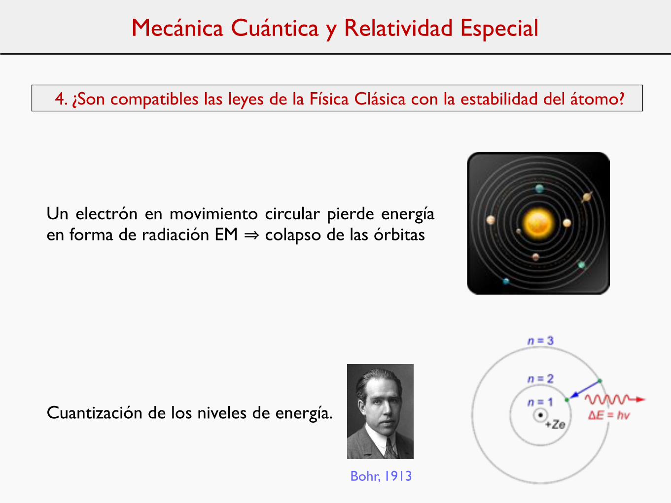
4. ¿Son compatibles las leyes de la Física Clásica con la estabilidad del átomo?
Un electrón en movimiento circular pierde energía en forma de radiación EM ⇒ colapso de las órbitas
Cuantización de los niveles de energía.
Bohr, 1913
Mecánica Cuántica y Relatividad Especial

5. ¿Cómo unir las ideas de Planck, Einstein y Bohr en una única estructura, consistente con la mecánica clásica?
Desarrollo de la Mecánica Cuántica
Bohr, Heisenberg, Pauli, Schrödinger, ... c.1915-1930
Explicación de la estructura de la materia a nivel atómico y molecular
Mecánica Cuántica y Relatividad Especial
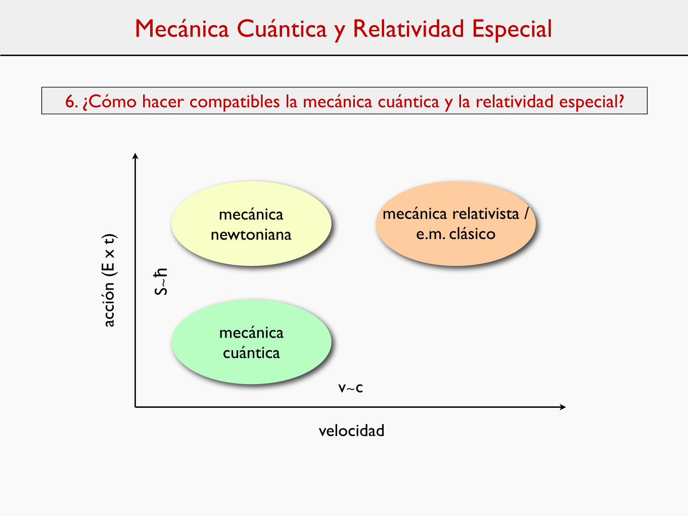
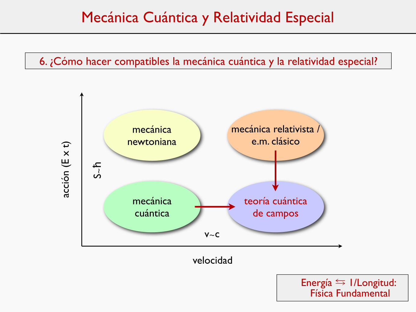
6. ¿Cómo hacer compatibles la mecánica cuántica y la relatividad especial?
velocidad
acci
ón (
E x
t)
v∼c
S∼ħ
mecánica newtoniana
mecánica relativista / e.m. clásico
mecánica cuántica
Mecánica Cuántica y Relatividad Especial
6. ¿Cómo hacer compatibles la mecánica cuántica y la relatividad especial?
velocidad
acci
ón (
E x
t)
v∼c
S∼ħ
mecánica newtoniana
mecánica relativista / e.m. clásico
mecánica cuántica
teoría cuántica de campos
Energía ⇆ 1/Longitud: Física Fundamental
Mecánica Cuántica y Relatividad Especial
Dirac: la Mecánica Cuántica Relativista
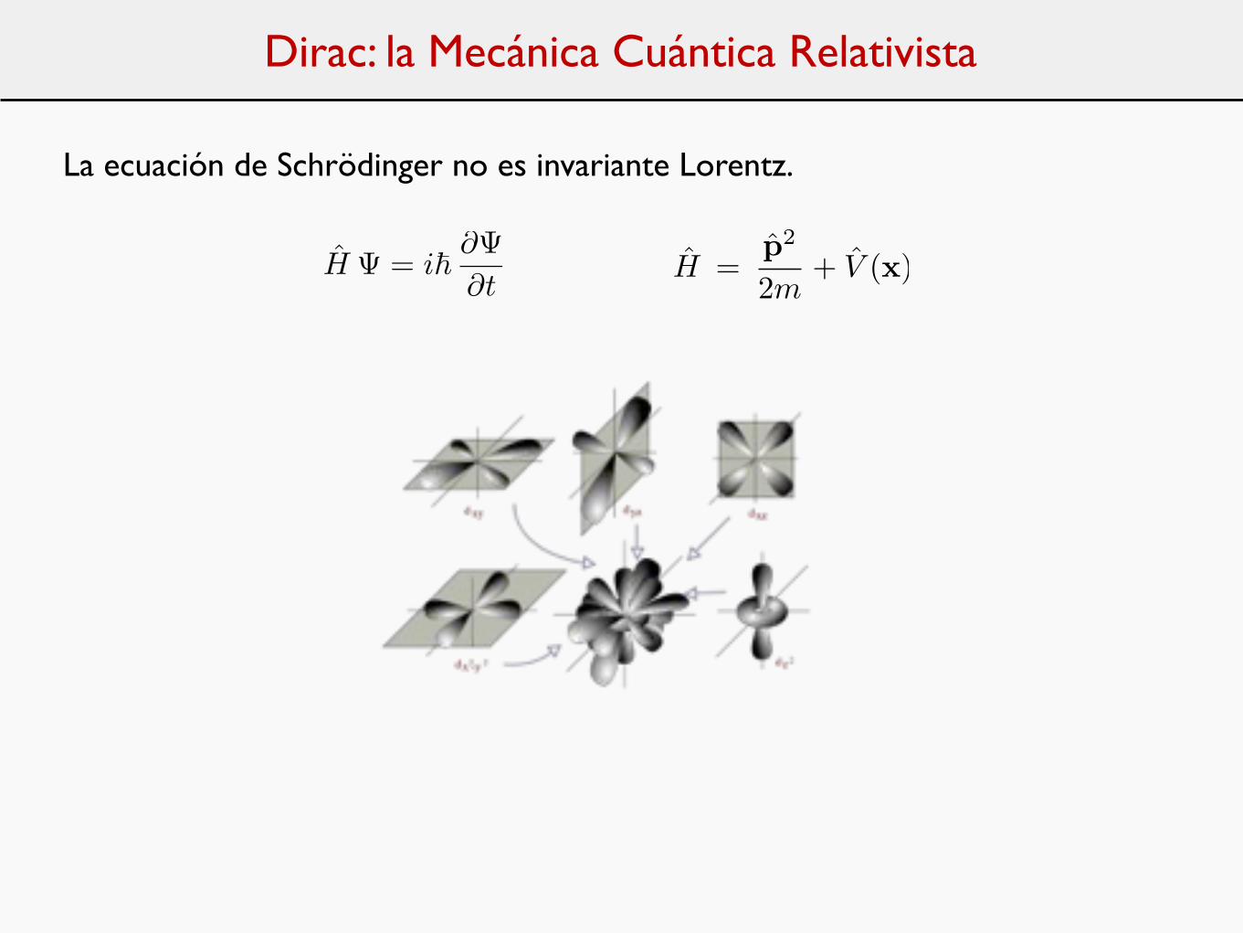
La ecuación de Schrödinger no es invariante Lorentz.
H Ψ = i� ∂Ψ∂t
H =p2
2m+ V (x)
Dirac: la Mecánica Cuántica Relativista
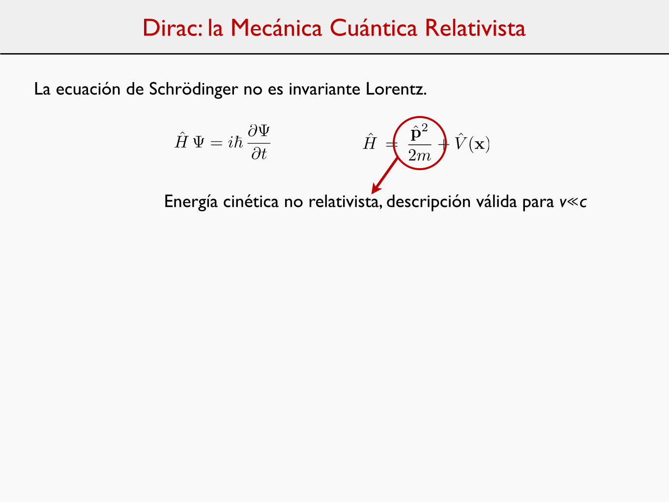
La ecuación de Schrödinger no es invariante Lorentz.
H Ψ = i� ∂Ψ∂t
H =p2
2m+ V (x)
Energía cinética no relativista, descripción válida para v≪c
Dirac: la Mecánica Cuántica Relativista
La ecuación de Schrödinger no es invariante Lorentz.
H Ψ = i� ∂Ψ∂t
H =p2
2m+ V (x)
Energía cinética no relativista, descripción válida para v≪c
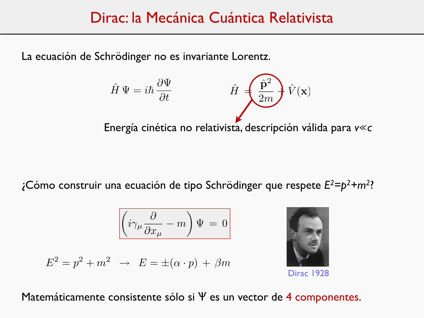
¿Cómo construir una ecuación de tipo Schrödinger que respete E2=p2+m2?
�iγµ
∂
∂xµ−m
�Ψ = 0
Dirac 1928
Matemáticamente consistente sólo si Ψ es un vector de 4 componentes.
E2 = p2 + m2 → E = ±(α · p) + βm
Dirac: la Mecánica Cuántica Relativista
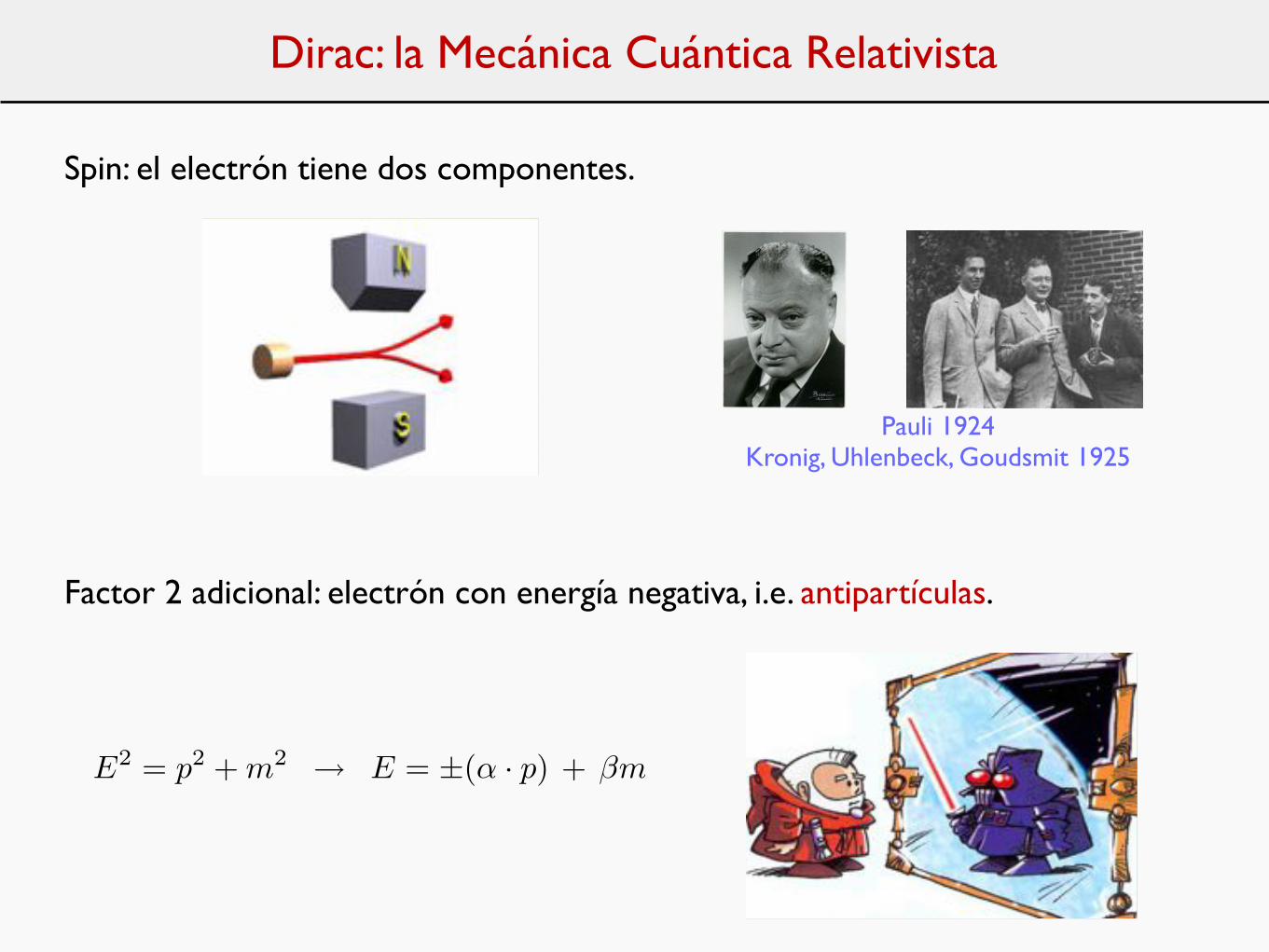
Spin: el electrón tiene dos componentes.
PARTÍCULAS ELEMENTALES1925
Spin
Fermiones y bosones
- Experimento de Stern-Gerlach (1922)Un campo magnético inhomogéneo desvía los electrones según su momento magnético (relacionado con el spin)
-Fermiones: Partículas con spin semi-entero (electrón, protón, etc)Principio de exclusión de Pauli: No pueden existir dos fermiones en el mismo estado cuántico
-Bosones: Partículas con spin entero (fotón, etc)No se aplica el principio de exclusión de Pauli.Sistemas de bosones en el mismo estado cuántico (p.ej. láser)
⇒ Impenetrabilidad de la materia
Estados de rotación intrínsecos de la partícula,polarización levógira o dextrógira de la onda !
(El átomo cuántico está todo lo “lleno” que puede estar de forma compatible con el principio de exclusión de Pauli)
Principio de exclusión de Pauli (1924): en cada orbital, sólo dos electrones, que se distinguen por un misterioso número cuántico bi-valuado Kronig; Uhlenbeck, Goudsmit (1925): “spin” +1/2, -1/2
Pauli 1924Kronig, Uhlenbeck, Goudsmit 1925
Factor 2 adicional: electrón con energía negativa, i.e. antipartículas.
E2 = p2 + m2 → E = ±(α · p) + βm
Relatividad Especial1928
E = p
2
2m! ih "
"t# = $ h2
2m %2#Compárese con la ecuación de Schrödinger
(no-relativista)
P.A.M. Dirac
E2 = p2 +m2 !
E = ±(" # p) + $ m
¡Predicción de la existencia de antipartículas!
Observación matemática: la generalización sólo existe si la partícula tiene cuatro grados de libertad
La ecuación de Dirac generaliza la de Schrödinger (p.ej. electrón) al régimen relativistaUnificación de relatividad y mecánica cuántica
Interpretación física: - Dos estados de spin - Dos estados corresponden a una partícula con igual masa y carga opuesta: antipartícula
Mecánica Cuántica
Relativista
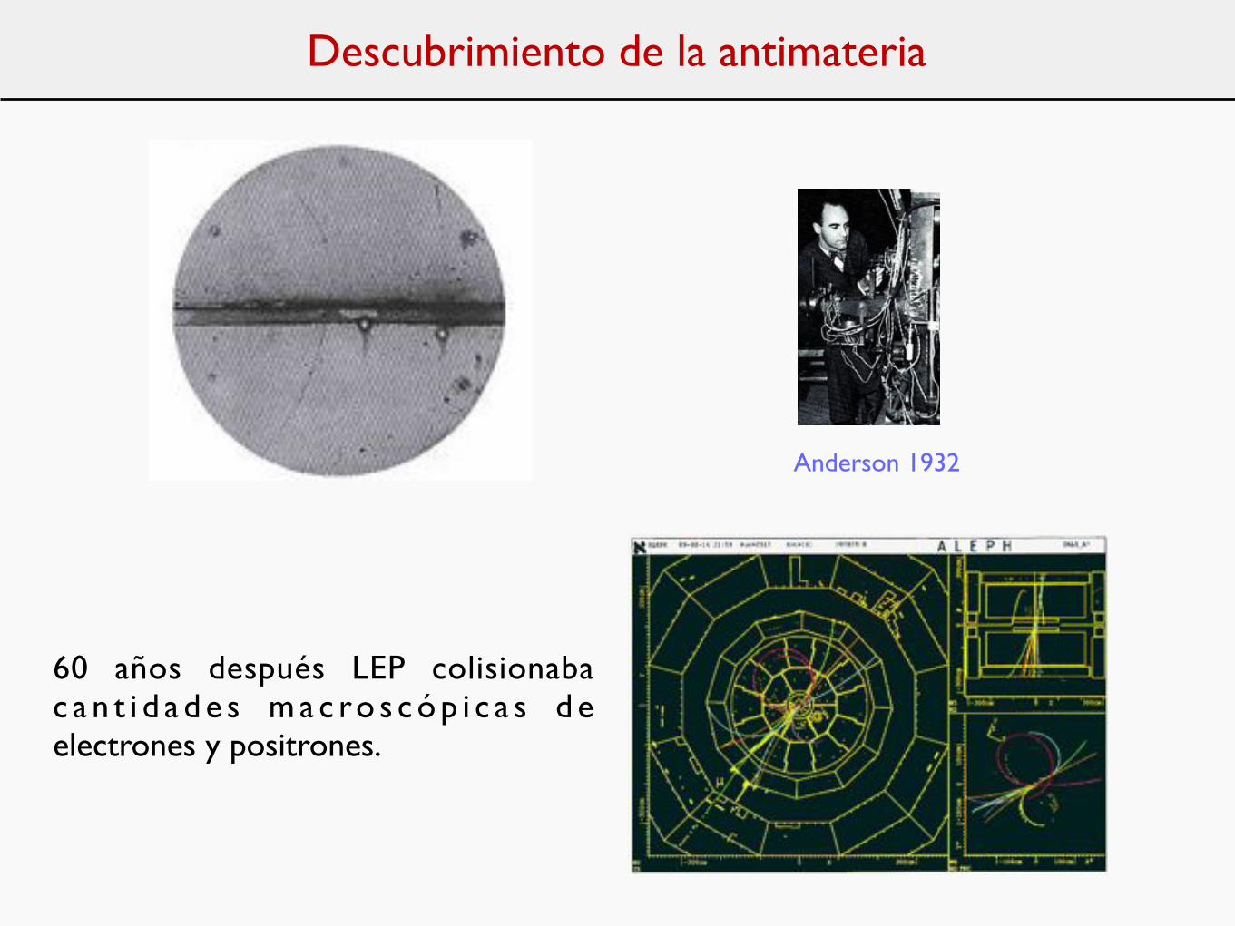
Descubrimiento de la antimateria
Anderson 1932
60 años después LEP colisionaba c a n t i d a d e s m a c ro s c ó p i c a s d e electrones y positrones.
La interacción nuclear débil: neutrinos
La formulación de Dirac de la materia relativista permitió avanzar muy rápidamente en el estudio de las interacciones fundamentales.
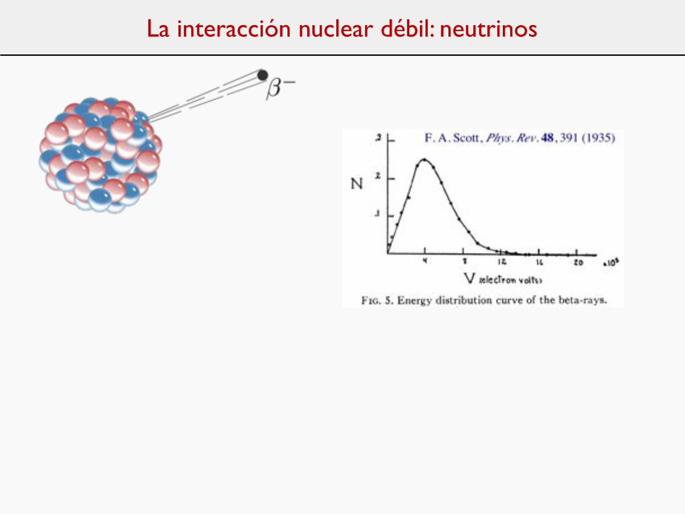
La interacción nuclear débil: neutrinos
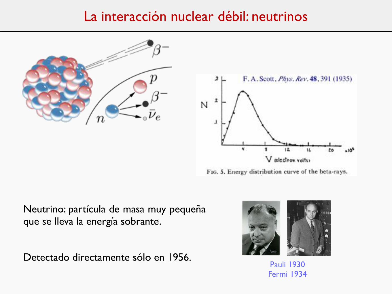
La interacción nuclear débil: neutrinos
Neutrino: partícula de masa muy pequeña que se lleva la energía sobrante.
Pauli 1930Fermi 1934
Detectado directamente sólo en 1956.
La interacción nuclear fuerte: mesones de Yukawa
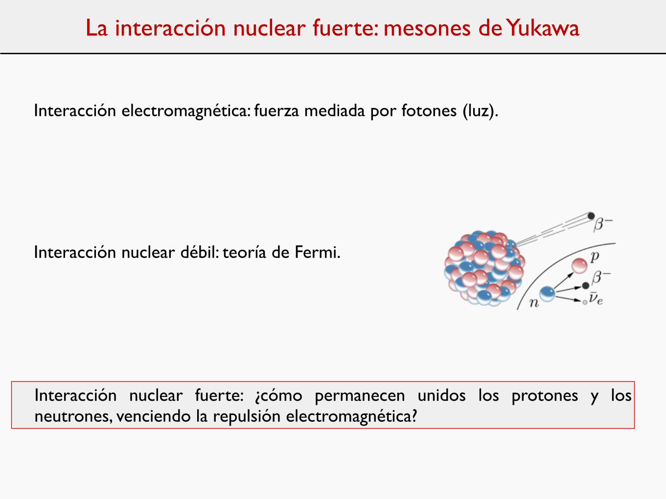
Interacción electromagnética: fuerza mediada por fotones (luz).
Interacción nuclear débil: teoría de Fermi.
Interacción nuclear fuerte: ¿cómo permanecen unidos los protones y los neutrones, venciendo la repulsión electromagnética?

La interacción nuclear fuerte: mesones de Yukawa
Interacción nuclear fuerte: ¿cómo permanecen unidos los protones y los neutrones, venciendo la repulsión electromagnética?
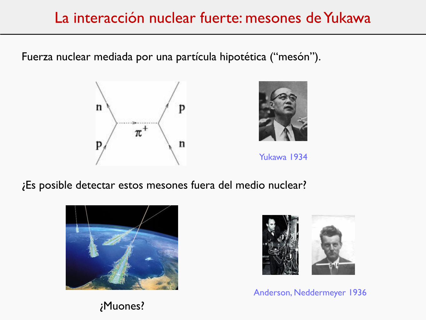
Fuerza nuclear mediada por una partícula hipotética (“mesón”).
Yukawa 1934
La interacción nuclear fuerte: mesones de Yukawa
Fuerza nuclear mediada por una partícula hipotética (“mesón”).
¿Es posible detectar estos mesones fuera del medio nuclear?
¿Muones?Anderson, Neddermeyer 1936
Yukawa 1934
La interacción nuclear fuerte: mesones de Yukawa
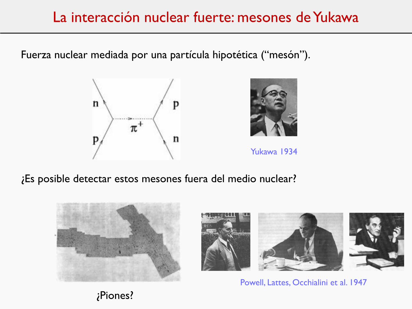
Fuerza nuclear mediada por una partícula hipotética (“mesón”).
¿Es posible detectar estos mesones fuera del medio nuclear?
¿Piones?Powell, Lattes, Occhialini et al. 1947
Yukawa 1934
19001910
1920
1930
1940
1950
1960
1970
1980
19902000
2010
CamposPartículasElectromagnético
Relatividad especial
Mecánica CuánticaOnda / partícula
Fermiones / Bosones
Dirac Antimateria
Bosones W
QED
Maxwell
Higgs
Supercuerdas?
Universo
NewtonMecánica Clásica,Teoría Cinética,Thermodinámica
MovimientoBrowniano
Relatividad General
Nucleosíntesis cosmológica
Inflación
Átomo
Núcleo
e-
p+
n
Zoo de partículas
u
µ -
!
"e
"µ
"!
d s
c
!-
!-
b
t
Galaxias ; Universo en expansión;
modelo del Big Bang
Fusión nuclear
Fondo de radiación de microondas
Masas de neutrinos
ColorQCD
Energía oscura
Materia oscura
W Zg
Fotón
Débil Fuerte
e+
p-
Desintegración betai Mesones
de Yukawa
Boltzmann
Radio-actividad
Tecnología
Geiger
Cámara de niebla
Cámara de burbujase
Ciclotrón
Detectores Aceleradores
Rayos cósmicos
Sincrotrón
Aceleradores e+e
Aceleradoresp+p-
Enfriamiento de haces
Online computers
WWW
GRID
Detectores modernos
Violación de P, C, CP
MODELO ESTÁNDAR
Unificación electrodébil
3 familias
Inhomgeneidades del fondo de microondas
1895
1905
Supersimetría?
Gran unificaci’on?
Cámara de hilos
Plan
Introducción: escalas de espacio y de energía en Física Fundamental.
Física Cuántica y Relatividad Especial.
Las preguntas revolucionarias.
Dirac y la Mecánica Cuántica Relativista.
Las interacciones nucleares débil y fuerte: neutrinos y mesones.
Interludio: diagramas de Feynman.
Teoría Cuántica de Campos.
Efectos cuánticos y fuerzas fundamentales.
Infinitos y Guerras.
La Edad de Plata: Electrodinámica Cuántica y leyes fundamentales.
Simetrías: la Edad de Oro.
El Camino Óctuple: Quarks.
La interacción electrodébil: corrientes neutras.
Más infinitos.
El Modelo Estándar de la Física de Partículas.

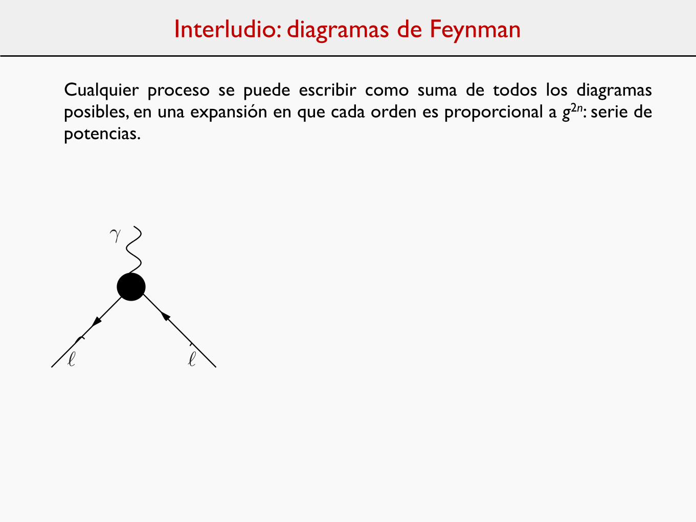
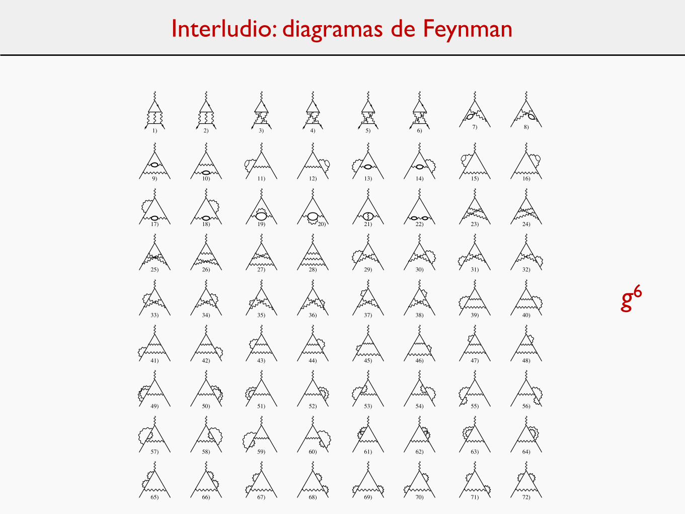
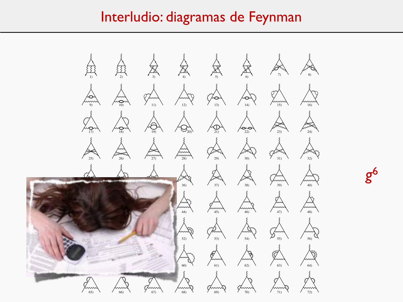
Interludio: diagramas de Feynman
Instrumento gráfico para entender interacciones (suficientemente débiles) como intercambio de partículas virtuales.
∆E ∆t ≥ �E = mc2
Feynman, c. 1944(Manhattan Project)
Interludio: diagramas de Feynman
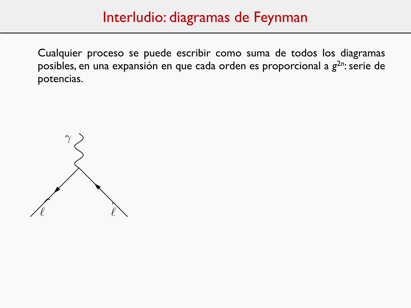
Cualquier proceso se puede escribir como suma de todos los diagramas posibles, en una expansión en que cada orden es proporcional a g2n: serie de potencias.
and later we will denote by
CL =3
!
k=1
A(2L)k , (46)
the total L–loop coe!cient of the (!/")L term. The present precision of the experimental result [16,92]
#aexpµ = 63 ! 10!11 , (47)
as well as the future prospects of possible improvements [111], which are expected to be able to reach
#afinµ " 10 ! 10!11 , (48)
determine the precision at which we need the theoretical prediction. For the n–loop coe!cients multiplying(!/")n the error Eq. (48) translates into the required accuracies: #C1 " 4 ! 10!8, #C2 " 1 ! 10!5, #C3 "7!10!3, #C4 " 3 and #C5 " 1!103 . To match the current accuracy one has to multiply all estimates witha factor 6, which is the experimental error in units of 10!10.
3.1. Universal Contributions
• According to Eq. (70) the leading order contribution Fig. 8 may be written in the form (see below)
a(2) QED! =
!
"
1"
0
dx (1 # x) =!
"
1
2, (49)
which is trivial to evaluate. This is the famous result of Schwinger from 1948 [52].
$
$
%%
Fig. 8. The universal lowest order QED contribution to a!.
• At two loops in QED there are the 9 diagrams shown in Fig. 9 which contribute to aµ. The first 6 diagrams,which have attached two virtual photons to the external muon string of lines contribute to the universalterm. They form a gauge invariant subset of diagrams and yield the result
A(4)1 [1!6] = #279
144+
5"2
12# "2
2ln 2 +
3
4&(3) .
The last 3 diagrams include photon vacuum polarization (vap / VP) due to the lepton loops. The one withthe muon loop is also universal in the sense that it contributes to the mass independent correction
A(4)1 vap(mµ/m! = 1) =
119
36# "2
3.
The complete “universal” part yields the coe!cient A(4)1 calculated first by Petermann [112] and by Som-
merfield [113] in 1957:
A(4)1 uni =
197
144+
"2
12# "2
2ln 2 +
3
4&(3) = #0.328 478 965 579 193 78... (50)
where &(n) is the Riemann &–function of argument n (see also [114]).
21
Interludio: diagramas de Feynman
Cualquier proceso se puede escribir como suma de todos los diagramas posibles, en una expansión en que cada orden es proporcional a g2n: serie de potencias.
and later we will denote by
CL =3
!
k=1
A(2L)k , (46)
the total L–loop coe!cient of the (!/")L term. The present precision of the experimental result [16,92]
#aexpµ = 63 ! 10!11 , (47)
as well as the future prospects of possible improvements [111], which are expected to be able to reach
#afinµ " 10 ! 10!11 , (48)
determine the precision at which we need the theoretical prediction. For the n–loop coe!cients multiplying(!/")n the error Eq. (48) translates into the required accuracies: #C1 " 4 ! 10!8, #C2 " 1 ! 10!5, #C3 "7!10!3, #C4 " 3 and #C5 " 1!103 . To match the current accuracy one has to multiply all estimates witha factor 6, which is the experimental error in units of 10!10.
3.1. Universal Contributions
• According to Eq. (70) the leading order contribution Fig. 8 may be written in the form (see below)
a(2) QED! =
!
"
1"
0
dx (1 # x) =!
"
1
2, (49)
which is trivial to evaluate. This is the famous result of Schwinger from 1948 [52].
$
$
%%
Fig. 8. The universal lowest order QED contribution to a!.
• At two loops in QED there are the 9 diagrams shown in Fig. 9 which contribute to aµ. The first 6 diagrams,which have attached two virtual photons to the external muon string of lines contribute to the universalterm. They form a gauge invariant subset of diagrams and yield the result
A(4)1 [1!6] = #279
144+
5"2
12# "2
2ln 2 +
3
4&(3) .
The last 3 diagrams include photon vacuum polarization (vap / VP) due to the lepton loops. The one withthe muon loop is also universal in the sense that it contributes to the mass independent correction
A(4)1 vap(mµ/m! = 1) =
119
36# "2
3.
The complete “universal” part yields the coe!cient A(4)1 calculated first by Petermann [112] and by Som-
merfield [113] in 1957:
A(4)1 uni =
197
144+
"2
12# "2
2ln 2 +
3
4&(3) = #0.328 478 965 579 193 78... (50)
where &(n) is the Riemann &–function of argument n (see also [114]).
21

Interludio: diagramas de Feynman
and later we will denote by
CL =3
!
k=1
A(2L)k , (46)
the total L–loop coe!cient of the (!/")L term. The present precision of the experimental result [16,92]
#aexpµ = 63 ! 10!11 , (47)
as well as the future prospects of possible improvements [111], which are expected to be able to reach
#afinµ " 10 ! 10!11 , (48)
determine the precision at which we need the theoretical prediction. For the n–loop coe!cients multiplying(!/")n the error Eq. (48) translates into the required accuracies: #C1 " 4 ! 10!8, #C2 " 1 ! 10!5, #C3 "7!10!3, #C4 " 3 and #C5 " 1!103 . To match the current accuracy one has to multiply all estimates witha factor 6, which is the experimental error in units of 10!10.
3.1. Universal Contributions
• According to Eq. (70) the leading order contribution Fig. 8 may be written in the form (see below)
a(2) QED! =
!
"
1"
0
dx (1 # x) =!
"
1
2, (49)
which is trivial to evaluate. This is the famous result of Schwinger from 1948 [52].
$
$
%%
Fig. 8. The universal lowest order QED contribution to a!.
• At two loops in QED there are the 9 diagrams shown in Fig. 9 which contribute to aµ. The first 6 diagrams,which have attached two virtual photons to the external muon string of lines contribute to the universalterm. They form a gauge invariant subset of diagrams and yield the result
A(4)1 [1!6] = #279
144+
5"2
12# "2
2ln 2 +
3
4&(3) .
The last 3 diagrams include photon vacuum polarization (vap / VP) due to the lepton loops. The one withthe muon loop is also universal in the sense that it contributes to the mass independent correction
A(4)1 vap(mµ/m! = 1) =
119
36# "2
3.
The complete “universal” part yields the coe!cient A(4)1 calculated first by Petermann [112] and by Som-
merfield [113] in 1957:
A(4)1 uni =
197
144+
"2
12# "2
2ln 2 +
3
4&(3) = #0.328 478 965 579 193 78... (50)
where &(n) is the Riemann &–function of argument n (see also [114]).
21
Cualquier proceso se puede escribir como suma de todos los diagramas posibles, en una expansión en que cada orden es proporcional a g2n: serie de potencias.
g gg2
A = A0 + A1g2 + A2g4 + A3g6 + ...
and later we will denote by
CL =3
!
k=1
A(2L)k , (46)
the total L–loop coe!cient of the (!/")L term. The present precision of the experimental result [16,92]
#aexpµ = 63 ! 10!11 , (47)
as well as the future prospects of possible improvements [111], which are expected to be able to reach
#afinµ " 10 ! 10!11 , (48)
determine the precision at which we need the theoretical prediction. For the n–loop coe!cients multiplying(!/")n the error Eq. (48) translates into the required accuracies: #C1 " 4 ! 10!8, #C2 " 1 ! 10!5, #C3 "7!10!3, #C4 " 3 and #C5 " 1!103 . To match the current accuracy one has to multiply all estimates witha factor 6, which is the experimental error in units of 10!10.
3.1. Universal Contributions
• According to Eq. (70) the leading order contribution Fig. 8 may be written in the form (see below)
a(2) QED! =
!
"
1"
0
dx (1 # x) =!
"
1
2, (49)
which is trivial to evaluate. This is the famous result of Schwinger from 1948 [52].
$
$
%%
Fig. 8. The universal lowest order QED contribution to a!.
• At two loops in QED there are the 9 diagrams shown in Fig. 9 which contribute to aµ. The first 6 diagrams,which have attached two virtual photons to the external muon string of lines contribute to the universalterm. They form a gauge invariant subset of diagrams and yield the result
A(4)1 [1!6] = #279
144+
5"2
12# "2
2ln 2 +
3
4&(3) .
The last 3 diagrams include photon vacuum polarization (vap / VP) due to the lepton loops. The one withthe muon loop is also universal in the sense that it contributes to the mass independent correction
A(4)1 vap(mµ/m! = 1) =
119
36# "2
3.
The complete “universal” part yields the coe!cient A(4)1 calculated first by Petermann [112] and by Som-
merfield [113] in 1957:
A(4)1 uni =
197
144+
"2
12# "2
2ln 2 +
3
4&(3) = #0.328 478 965 579 193 78... (50)
where &(n) is the Riemann &–function of argument n (see also [114]).
21
g0
Interludio: diagramas de Feynman
1) 2) 3)
4) 5) 6)
7) 8) 9)! !µ e "
µ
!
Fig. 9. Diagrams 1-7 represent the universal second order contribution to aµ, diagram 8 yields the “light”, diagram 9 the“heavy” mass dependent corrections.
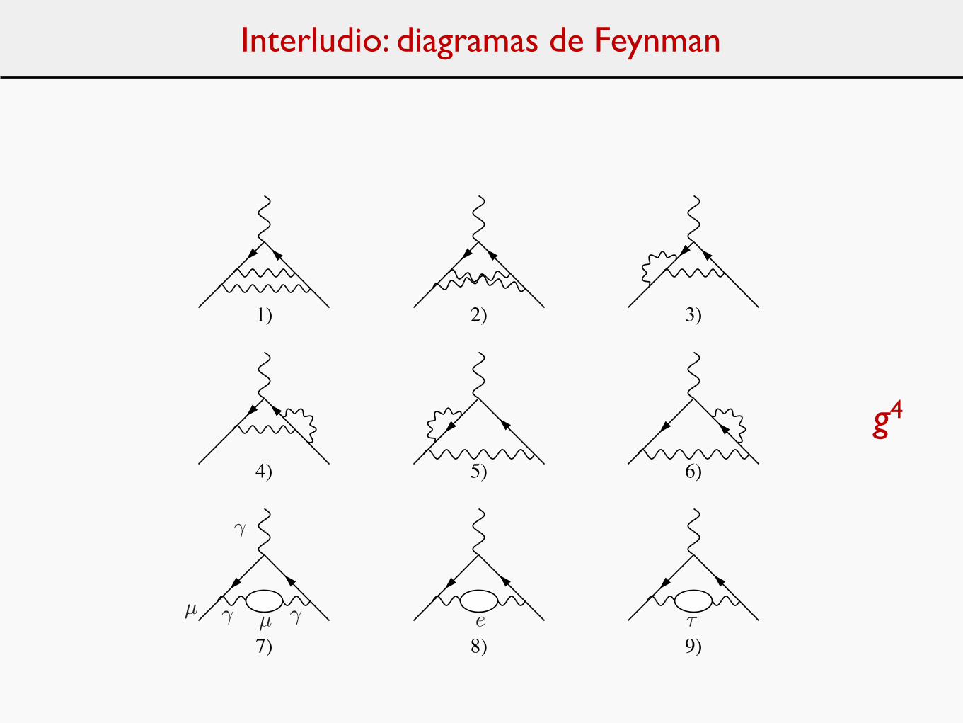
• At three loops in QED there are the 72 diagrams shown in Fig. 10 contributing to g ! 2 of the muon. Inclosed fermion loops any of the SM fermions may circulate. The gauge invariant subset of 72 diagrams where
all closed fermion loops are muon–loops yield the universal one–flavor QED contribution A(6)1 uni. This set
has been calculated analytically mainly by Remiddi and his collaborators [115], and Laporta and Remiddiobtained the final result in 1996 after finding a trick to calculate the non–planar “triple cross” topologydiagram 25) of Fig. 10 [116] (see also [117]). The result turned out to be surprisingly compact and reads
A(6)1 uni =
28259
5184+
17101
810#2 ! 298
9#2 ln 2 +
139
18$(3) +
100
3
!
Li4(1
2) +
1
24ln4 2 ! 1
24#2 ln2 2
"
! 239
2160#4 +
83
72#2$(3) ! 215
24$(5) = 1.181 241 456 587 . . . (51)
This famous analytical result largely confirmed an earlier numerical calculation by Kinoshita [117]. Theconstants needed for the evaluation of Eq. (51) are given in Eqs. (A.13) and (A.14).
The big advantage of the analytic result is that it allows a numerical evaluation at any desired precision.The direct numerical evaluation of the multidimensional Feynman integrals by Monte Carlo methods isalways of limited precision and an improvement is always very expensive in computing power.• At four loops there are 891 diagrams [373 have closed lepton loops (see Fig. 11), 518 without fermionloops=gauge invariant set Group V (see Fig. 12)] with common fermion lines. Their contribution has beencalculated by numerical methods by Kinoshita and collaborators. The calculation of the 4–loop contributionto aµ is a formidable task. Since the individual diagrams are much more complicated than the 3–loop ones,only a few have been calculated analytically so far [118]–[120]. In most cases one has to resort to numericalcalculations. This approach has been developed and perfected over the past 25 years by Kinoshita and hiscollaborators [121]–[125] with the very recent recalculations and improvements [108,126,39]. As a result ofthe enduring heroic e!ort an improved answer has been obtained recently by Aoyama, Hayakawa, Kinoshitaand Nio [108] who find
A(8)1 = !1.9144(35) (52)
where the error is due to the Monte Carlo integration. This very recent result is correcting the one published
before in [127] and shifting the coe"cient of the#
!"
$4term by – 0.19 (10%). Some error in the cancellation
of IR singular terms was found in calculating diagrams M18 (!0.2207(210)) and M16 (+0.0274(235)) in the
22
g4
Interludio: diagramas de Feynman
1) 2) 3) 4) 5) 6) 7) 8)
9) 10) 11) 12) 13) 14) 15) 16)
17) 18) 19) 20) 21) 22) 23) 24)
25) 26) 27) 28) 29) 30) 31) 32)
33) 34) 35) 36) 37) 38) 39) 40)
41) 42) 43) 44) 45) 46) 47) 48)
49) 50) 51) 52) 53) 54) 55) 56)
57) 58) 59) 60) 61) 62) 63) 64)
65) 66) 67) 68) 69) 70) 71) 72)
Fig. 10. The universal third order contribution to aµ. All fermion loops here are muon–loops. Graphs 1) to 6) are the light–by—light scattering diagrams. Graphs 7) to 22) include photon vacuum polarization insertions. All non–universal contributions followby replacing at least one muon in a closed loop by some other fermion.
set of diagrams Fig. 12. The latter 518 diagrams without fermion loops also are responsible for the largestpart of the uncertainty in Eq. (52). Note that the universal O(!4) contribution is sizable, about 6 standarddeviations at current experimental accuracy, and a precise knowledge of this term is absolutely crucial forthe comparison between theory and experiment.• The universal 5–loop QED contribution is still largely unknown. Using the recipe proposed in Ref. [37],one obtains the following bound
A(10)1 = 0.0(4.6) , (53)
for the universal part as an estimate for the missing higher order terms.As a result the universal QED contribution may be written as
auni! = 0.5
!!
"
"
! 0.328 478 965 579 193 78 . . .!!
"
"2
+1.181 241 456 587 . . .!!
"
"3! 1.9144(35)
!!
"
"4+ 0.0(4.6)
!!
"
"5
23
g6
Plan
Introducción: escalas de espacio y de energía en Física Fundamental.
Física Cuántica y Relatividad Especial.
Las preguntas revolucionarias.
Dirac y la Mecánica Cuántica Relativista.
Las interacciones nucleares débil y fuerte: neutrinos y mesones.
Interludio: diagramas de Feynman.
Teoría Cuántica de Campos.
Efectos cuánticos y fuerzas fundamentales.
Infinitos y Guerras.
La Edad de Plata: Electrodinámica Cuántica y leyes fundamentales.
Simetrías: la Edad de Oro.
El Camino Óctuple: Quarks.
La interacción electrodébil: corrientes neutras.
Más infinitos.
El Modelo Estándar de la Física de Partículas.
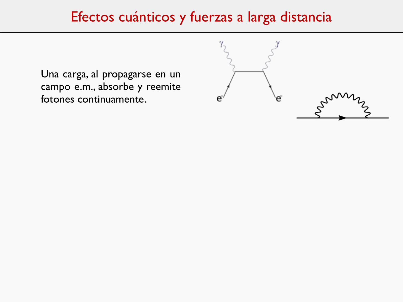
Efectos cuánticos y fuerzas a larga distancia
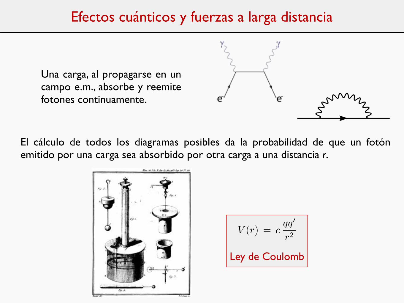
Una carga, al propagarse en un campo e.m., absorbe y reemite fotones continuamente.
Efectos cuánticos y fuerzas a larga distancia
Una carga, al propagarse en un campo e.m., absorbe y reemite fotones continuamente.
El cálculo de todos los diagramas posibles da la probabilidad de que un fotón emitido por una carga sea absorbido por otra carga a una distancia r.
V (r) = cqq�
r2
Ley de Coulomb
V (r) = −g2 e−mr
r
Efectos cuánticos y fuerzas a larga distancia
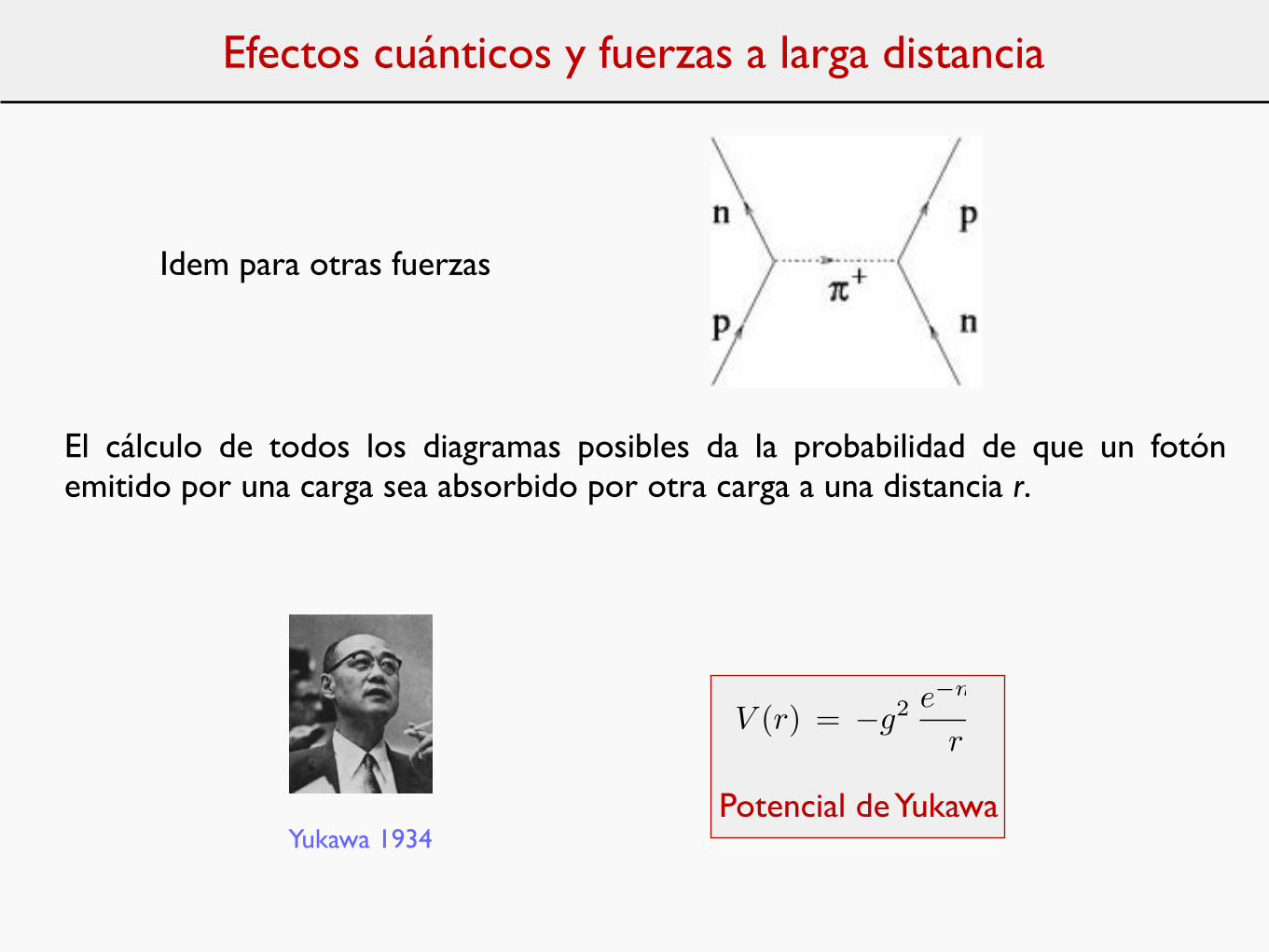
Idem para otras fuerzas
El cálculo de todos los diagramas posibles da la probabilidad de que un fotón emitido por una carga sea absorbido por otra carga a una distancia r.
Potencial de YukawaYukawa 1934
Infinitos y Guerras
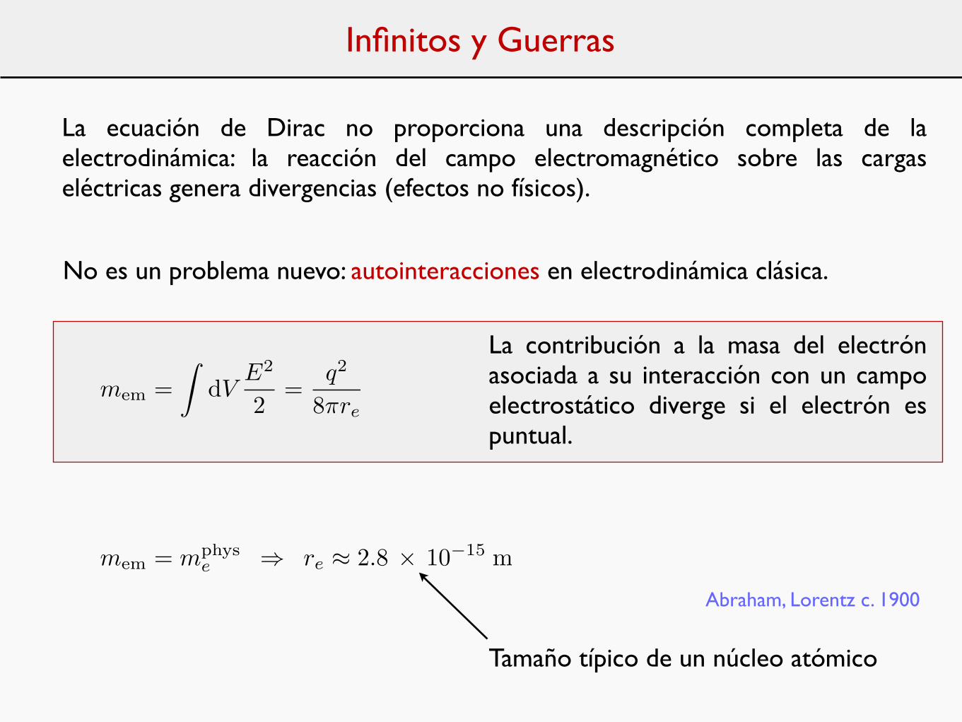
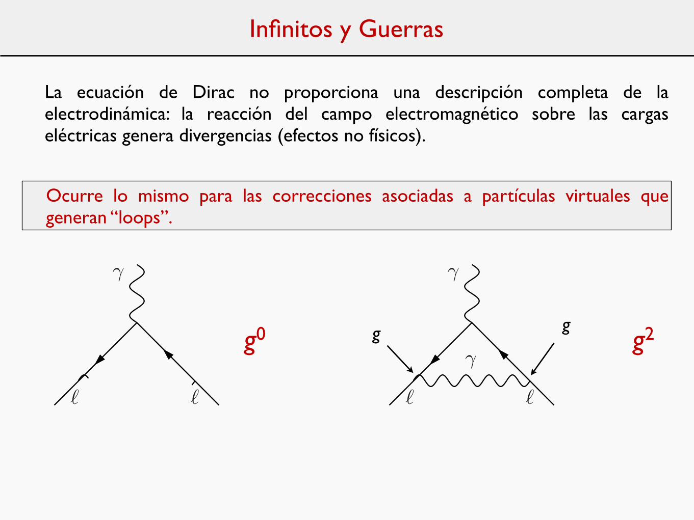
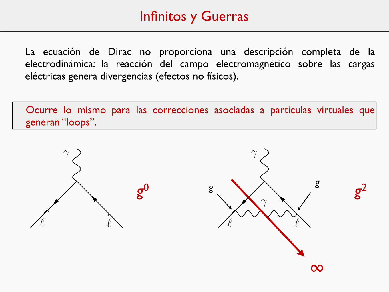
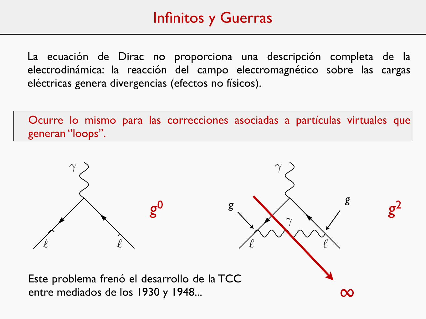
La ecuación de Dirac no proporciona una descripción completa de la electrodinámica: la reacción del campo electromagnético sobre las cargas eléctricas genera divergencias (efectos no físicos).
Infinitos y Guerras
La ecuación de Dirac no proporciona una descripción completa de la electrodinámica: la reacción del campo electromagnético sobre las cargas eléctricas genera divergencias (efectos no físicos).
No es un problema nuevo: autointeracciones en electrodinámica clásica.
mem =�
dVE2
2=
q2
8πre
La contribución a la masa del electrón asociada a su interacción con un campo electrostático diverge si el electrón es puntual.
mem = mphyse ⇒ re ≈ 2.8 × 10⁻¹⁵ m
Tamaño típico de un núcleo atómico
Abraham, Lorentz c. 1900
Infinitos y Guerras
La ecuación de Dirac no proporciona una descripción completa de la electrodinámica: la reacción del campo electromagnético sobre las cargas eléctricas genera divergencias (efectos no físicos).
Ocurre lo mismo para las correcciones asociadas a partículas virtuales que generan “loops”.
and later we will denote by
CL =3
!
k=1
A(2L)k , (46)
the total L–loop coe!cient of the (!/")L term. The present precision of the experimental result [16,92]
#aexpµ = 63 ! 10!11 , (47)
as well as the future prospects of possible improvements [111], which are expected to be able to reach
#afinµ " 10 ! 10!11 , (48)
determine the precision at which we need the theoretical prediction. For the n–loop coe!cients multiplying(!/")n the error Eq. (48) translates into the required accuracies: #C1 " 4 ! 10!8, #C2 " 1 ! 10!5, #C3 "7!10!3, #C4 " 3 and #C5 " 1!103 . To match the current accuracy one has to multiply all estimates witha factor 6, which is the experimental error in units of 10!10.
3.1. Universal Contributions
• According to Eq. (70) the leading order contribution Fig. 8 may be written in the form (see below)
a(2) QED! =
!
"
1"
0
dx (1 # x) =!
"
1
2, (49)
which is trivial to evaluate. This is the famous result of Schwinger from 1948 [52].
$
$
%%
Fig. 8. The universal lowest order QED contribution to a!.
• At two loops in QED there are the 9 diagrams shown in Fig. 9 which contribute to aµ. The first 6 diagrams,which have attached two virtual photons to the external muon string of lines contribute to the universalterm. They form a gauge invariant subset of diagrams and yield the result
A(4)1 [1!6] = #279
144+
5"2
12# "2
2ln 2 +
3
4&(3) .
The last 3 diagrams include photon vacuum polarization (vap / VP) due to the lepton loops. The one withthe muon loop is also universal in the sense that it contributes to the mass independent correction
A(4)1 vap(mµ/m! = 1) =
119
36# "2
3.
The complete “universal” part yields the coe!cient A(4)1 calculated first by Petermann [112] and by Som-
merfield [113] in 1957:
A(4)1 uni =
197
144+
"2
12# "2
2ln 2 +
3
4&(3) = #0.328 478 965 579 193 78... (50)
where &(n) is the Riemann &–function of argument n (see also [114]).
21
g gg2
and later we will denote by
CL =3
!
k=1
A(2L)k , (46)
the total L–loop coe!cient of the (!/")L term. The present precision of the experimental result [16,92]
#aexpµ = 63 ! 10!11 , (47)
as well as the future prospects of possible improvements [111], which are expected to be able to reach
#afinµ " 10 ! 10!11 , (48)
determine the precision at which we need the theoretical prediction. For the n–loop coe!cients multiplying(!/")n the error Eq. (48) translates into the required accuracies: #C1 " 4 ! 10!8, #C2 " 1 ! 10!5, #C3 "7!10!3, #C4 " 3 and #C5 " 1!103 . To match the current accuracy one has to multiply all estimates witha factor 6, which is the experimental error in units of 10!10.
3.1. Universal Contributions
• According to Eq. (70) the leading order contribution Fig. 8 may be written in the form (see below)
a(2) QED! =
!
"
1"
0
dx (1 # x) =!
"
1
2, (49)
which is trivial to evaluate. This is the famous result of Schwinger from 1948 [52].
$
$
%%
Fig. 8. The universal lowest order QED contribution to a!.
• At two loops in QED there are the 9 diagrams shown in Fig. 9 which contribute to aµ. The first 6 diagrams,which have attached two virtual photons to the external muon string of lines contribute to the universalterm. They form a gauge invariant subset of diagrams and yield the result
A(4)1 [1!6] = #279
144+
5"2
12# "2
2ln 2 +
3
4&(3) .
The last 3 diagrams include photon vacuum polarization (vap / VP) due to the lepton loops. The one withthe muon loop is also universal in the sense that it contributes to the mass independent correction
A(4)1 vap(mµ/m! = 1) =
119
36# "2
3.
The complete “universal” part yields the coe!cient A(4)1 calculated first by Petermann [112] and by Som-
merfield [113] in 1957:
A(4)1 uni =
197
144+
"2
12# "2
2ln 2 +
3
4&(3) = #0.328 478 965 579 193 78... (50)
where &(n) is the Riemann &–function of argument n (see also [114]).
21
g0
∞
Infinitos y Guerras
La ecuación de Dirac no proporciona una descripción completa de la electrodinámica: la reacción del campo electromagnético sobre las cargas eléctricas genera divergencias (efectos no físicos).
Ocurre lo mismo para las correcciones asociadas a partículas virtuales que generan “loops”.
and later we will denote by
CL =3
!
k=1
A(2L)k , (46)
the total L–loop coe!cient of the (!/")L term. The present precision of the experimental result [16,92]
#aexpµ = 63 ! 10!11 , (47)
as well as the future prospects of possible improvements [111], which are expected to be able to reach
#afinµ " 10 ! 10!11 , (48)
determine the precision at which we need the theoretical prediction. For the n–loop coe!cients multiplying(!/")n the error Eq. (48) translates into the required accuracies: #C1 " 4 ! 10!8, #C2 " 1 ! 10!5, #C3 "7!10!3, #C4 " 3 and #C5 " 1!103 . To match the current accuracy one has to multiply all estimates witha factor 6, which is the experimental error in units of 10!10.
3.1. Universal Contributions
• According to Eq. (70) the leading order contribution Fig. 8 may be written in the form (see below)
a(2) QED! =
!
"
1"
0
dx (1 # x) =!
"
1
2, (49)
which is trivial to evaluate. This is the famous result of Schwinger from 1948 [52].
$
$
%%
Fig. 8. The universal lowest order QED contribution to a!.
• At two loops in QED there are the 9 diagrams shown in Fig. 9 which contribute to aµ. The first 6 diagrams,which have attached two virtual photons to the external muon string of lines contribute to the universalterm. They form a gauge invariant subset of diagrams and yield the result
A(4)1 [1!6] = #279
144+
5"2
12# "2
2ln 2 +
3
4&(3) .
The last 3 diagrams include photon vacuum polarization (vap / VP) due to the lepton loops. The one withthe muon loop is also universal in the sense that it contributes to the mass independent correction
A(4)1 vap(mµ/m! = 1) =
119
36# "2
3.
The complete “universal” part yields the coe!cient A(4)1 calculated first by Petermann [112] and by Som-
merfield [113] in 1957:
A(4)1 uni =
197
144+
"2
12# "2
2ln 2 +
3
4&(3) = #0.328 478 965 579 193 78... (50)
where &(n) is the Riemann &–function of argument n (see also [114]).
21
g gg2
and later we will denote by
CL =3
!
k=1
A(2L)k , (46)
the total L–loop coe!cient of the (!/")L term. The present precision of the experimental result [16,92]
#aexpµ = 63 ! 10!11 , (47)
as well as the future prospects of possible improvements [111], which are expected to be able to reach
#afinµ " 10 ! 10!11 , (48)
determine the precision at which we need the theoretical prediction. For the n–loop coe!cients multiplying(!/")n the error Eq. (48) translates into the required accuracies: #C1 " 4 ! 10!8, #C2 " 1 ! 10!5, #C3 "7!10!3, #C4 " 3 and #C5 " 1!103 . To match the current accuracy one has to multiply all estimates witha factor 6, which is the experimental error in units of 10!10.
3.1. Universal Contributions
• According to Eq. (70) the leading order contribution Fig. 8 may be written in the form (see below)
a(2) QED! =
!
"
1"
0
dx (1 # x) =!
"
1
2, (49)
which is trivial to evaluate. This is the famous result of Schwinger from 1948 [52].
$
$
%%
Fig. 8. The universal lowest order QED contribution to a!.
• At two loops in QED there are the 9 diagrams shown in Fig. 9 which contribute to aµ. The first 6 diagrams,which have attached two virtual photons to the external muon string of lines contribute to the universalterm. They form a gauge invariant subset of diagrams and yield the result
A(4)1 [1!6] = #279
144+
5"2
12# "2
2ln 2 +
3
4&(3) .
The last 3 diagrams include photon vacuum polarization (vap / VP) due to the lepton loops. The one withthe muon loop is also universal in the sense that it contributes to the mass independent correction
A(4)1 vap(mµ/m! = 1) =
119
36# "2
3.
The complete “universal” part yields the coe!cient A(4)1 calculated first by Petermann [112] and by Som-
merfield [113] in 1957:
A(4)1 uni =
197
144+
"2
12# "2
2ln 2 +
3
4&(3) = #0.328 478 965 579 193 78... (50)
where &(n) is the Riemann &–function of argument n (see also [114]).
21
g0
∞Este problema frenó el desarrollo de la TCC entre mediados de los 1930 y 1948...
Infinitos y Guerras
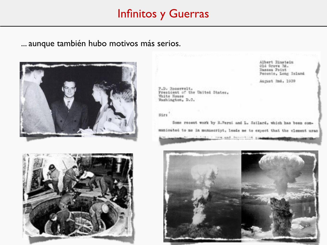
... aunque también hubo motivos más serios.
Renormalización: la Teoría Cuántica de Campos
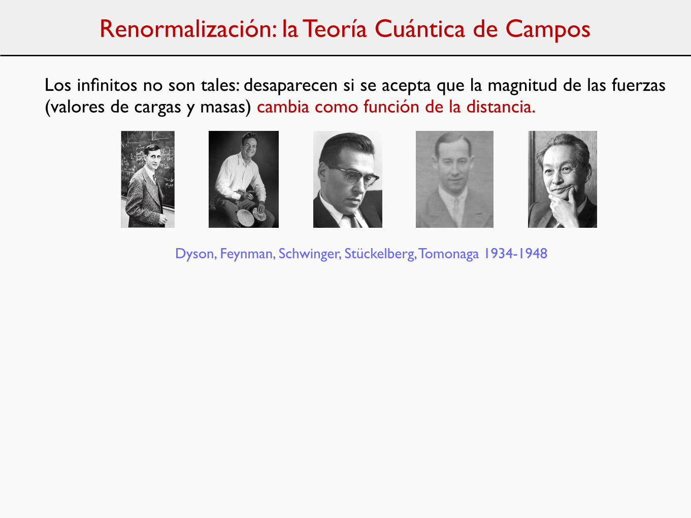
Los infinitos no son tales: desaparecen si se acepta que la magnitud de las fuerzas (valores de cargas y masas) cambia como función de la distancia.
Dyson, Feynman, Schwinger, Stückelberg, Tomonaga 1934-1948
Renormalización: la Teoría Cuántica de Campos
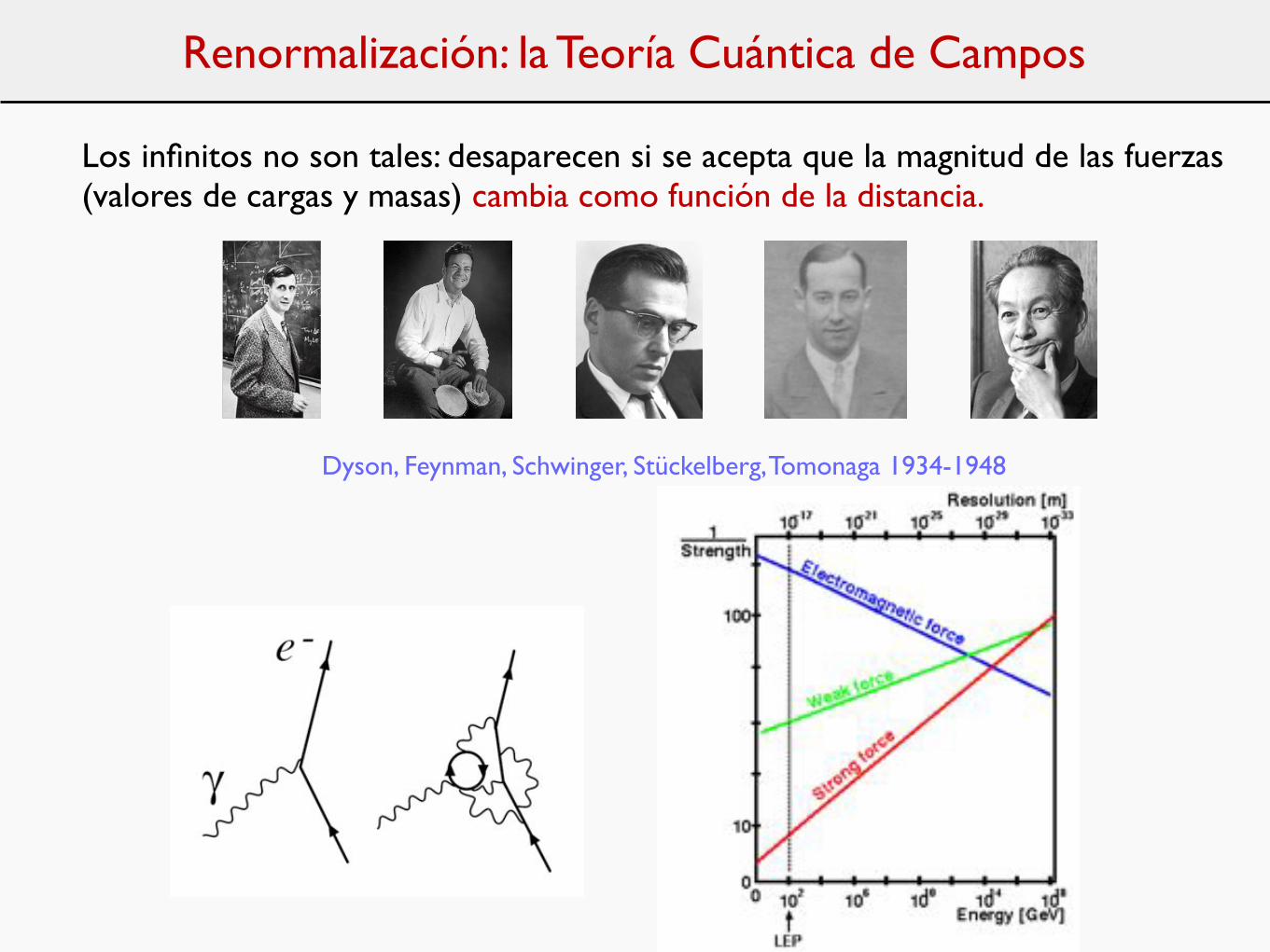
Los infinitos no son tales: desaparecen si se acepta que la magnitud de las fuerzas (valores de cargas y masas) cambia como función de la distancia.
Dyson, Feynman, Schwinger, Stückelberg, Tomonaga 1934-1948
Running coupling
αeff(r)
log(r)
|�F (r)| =αeff(r)
r2
r = 2× 10⁻¹² m
Renormalización: la Teoría Cuántica de Campos
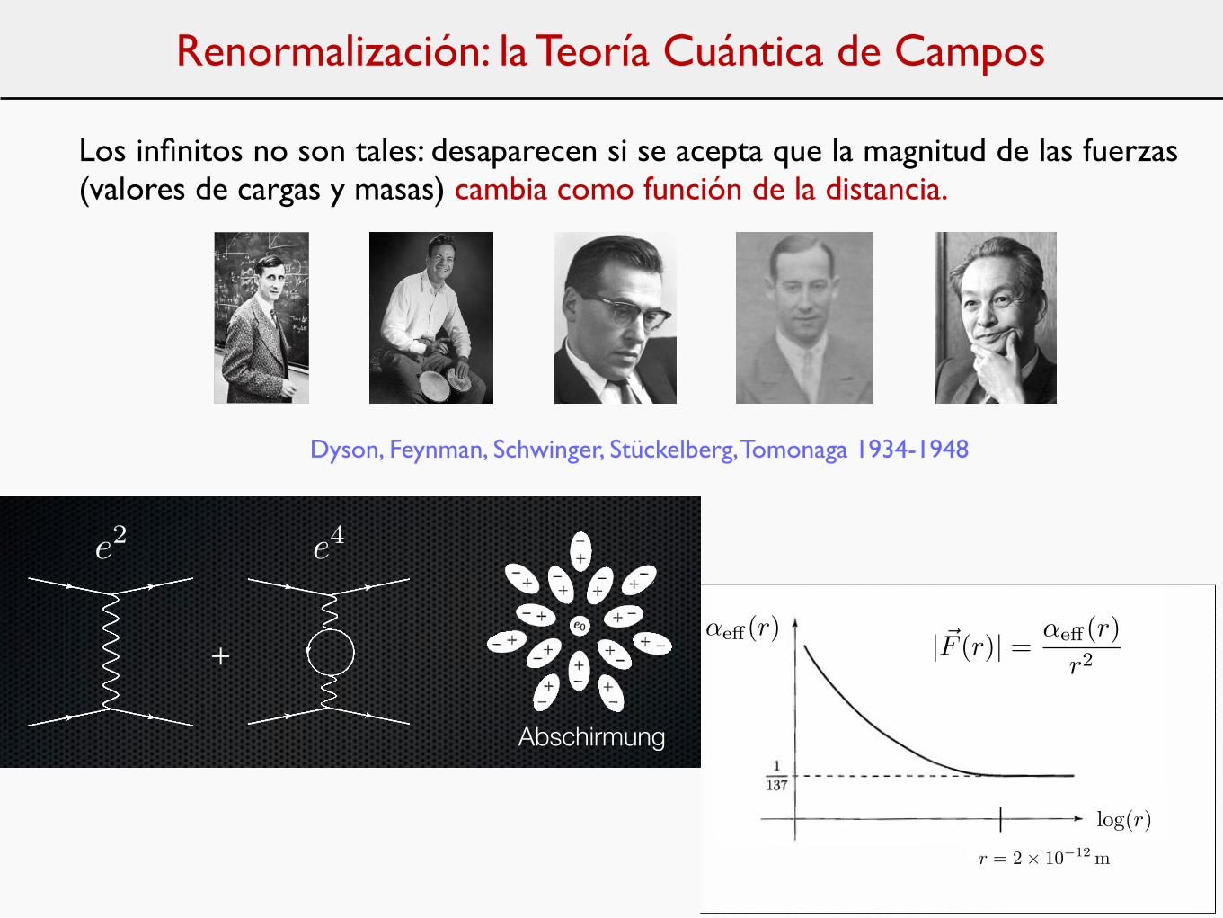
Los infinitos no son tales: desaparecen si se acepta que la magnitud de las fuerzas (valores de cargas y masas) cambia como función de la distancia.
Dyson, Feynman, Schwinger, Stückelberg, Tomonaga 1934-1948Vakuumpolarisation
Der zweite Beitrag ist ein kleiner Quanteneffekt
Er bewirkt, dass die Kraft bei sehr kurzen Distanzen etwas stärker als 1/r2 anwächst.
+
e2 e4
Abschirmung
Renormalización: la Teoría Cuántica de Campos
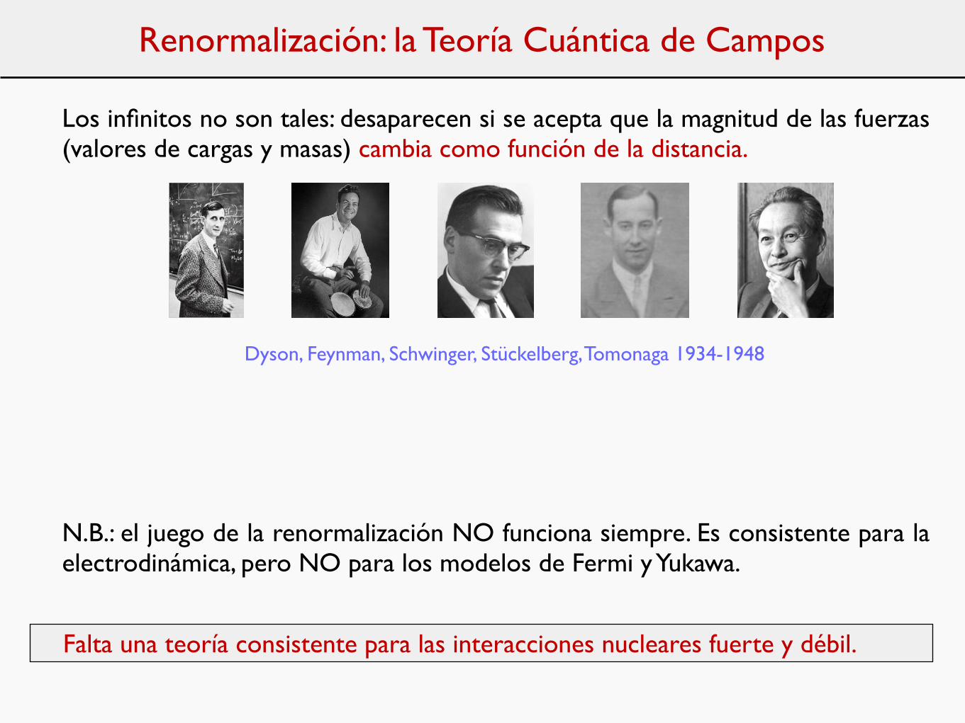
Los infinitos no son tales: desaparecen si se acepta que la magnitud de las fuerzas (valores de cargas y masas) cambia como función de la distancia.
Dyson, Feynman, Schwinger, Stückelberg, Tomonaga 1934-1948
N.B.: el juego de la renormalización NO funciona siempre. Es consistente para la electrodinámica, pero NO para los modelos de Fermi y Yukawa.
Falta una teoría consistente para las interacciones nucleares fuerte y débil.
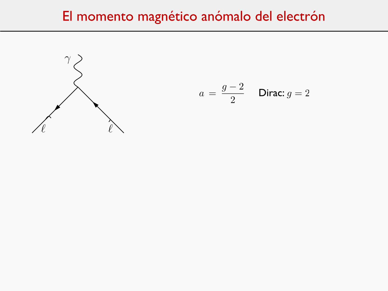
El momento magnético anómalo del electrón
and later we will denote by
CL =3
!
k=1
A(2L)k , (46)
the total L–loop coe!cient of the (!/")L term. The present precision of the experimental result [16,92]
#aexpµ = 63 ! 10!11 , (47)
as well as the future prospects of possible improvements [111], which are expected to be able to reach
#afinµ " 10 ! 10!11 , (48)
determine the precision at which we need the theoretical prediction. For the n–loop coe!cients multiplying(!/")n the error Eq. (48) translates into the required accuracies: #C1 " 4 ! 10!8, #C2 " 1 ! 10!5, #C3 "7!10!3, #C4 " 3 and #C5 " 1!103 . To match the current accuracy one has to multiply all estimates witha factor 6, which is the experimental error in units of 10!10.
3.1. Universal Contributions
• According to Eq. (70) the leading order contribution Fig. 8 may be written in the form (see below)
a(2) QED! =
!
"
1"
0
dx (1 # x) =!
"
1
2, (49)
which is trivial to evaluate. This is the famous result of Schwinger from 1948 [52].
$
$
%%
Fig. 8. The universal lowest order QED contribution to a!.
• At two loops in QED there are the 9 diagrams shown in Fig. 9 which contribute to aµ. The first 6 diagrams,which have attached two virtual photons to the external muon string of lines contribute to the universalterm. They form a gauge invariant subset of diagrams and yield the result
A(4)1 [1!6] = #279
144+
5"2
12# "2
2ln 2 +
3
4&(3) .
The last 3 diagrams include photon vacuum polarization (vap / VP) due to the lepton loops. The one withthe muon loop is also universal in the sense that it contributes to the mass independent correction
A(4)1 vap(mµ/m! = 1) =
119
36# "2
3.
The complete “universal” part yields the coe!cient A(4)1 calculated first by Petermann [112] and by Som-
merfield [113] in 1957:
A(4)1 uni =
197
144+
"2
12# "2
2ln 2 +
3
4&(3) = #0.328 478 965 579 193 78... (50)
where &(n) is the Riemann &–function of argument n (see also [114]).
21
a =g − 2
2g = 2Dirac:
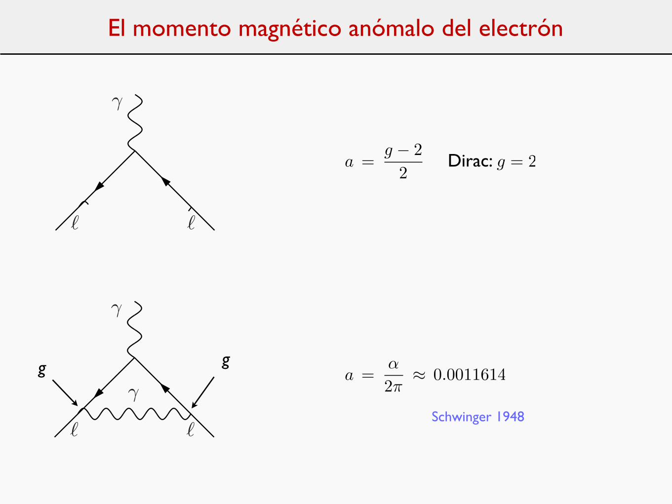
and later we will denote by
CL =3
!
k=1
A(2L)k , (46)
the total L–loop coe!cient of the (!/")L term. The present precision of the experimental result [16,92]
#aexpµ = 63 ! 10!11 , (47)
as well as the future prospects of possible improvements [111], which are expected to be able to reach
#afinµ " 10 ! 10!11 , (48)
determine the precision at which we need the theoretical prediction. For the n–loop coe!cients multiplying(!/")n the error Eq. (48) translates into the required accuracies: #C1 " 4 ! 10!8, #C2 " 1 ! 10!5, #C3 "7!10!3, #C4 " 3 and #C5 " 1!103 . To match the current accuracy one has to multiply all estimates witha factor 6, which is the experimental error in units of 10!10.
3.1. Universal Contributions
• According to Eq. (70) the leading order contribution Fig. 8 may be written in the form (see below)
a(2) QED! =
!
"
1"
0
dx (1 # x) =!
"
1
2, (49)
which is trivial to evaluate. This is the famous result of Schwinger from 1948 [52].
$
$
%%
Fig. 8. The universal lowest order QED contribution to a!.
• At two loops in QED there are the 9 diagrams shown in Fig. 9 which contribute to aµ. The first 6 diagrams,which have attached two virtual photons to the external muon string of lines contribute to the universalterm. They form a gauge invariant subset of diagrams and yield the result
A(4)1 [1!6] = #279
144+
5"2
12# "2
2ln 2 +
3
4&(3) .
The last 3 diagrams include photon vacuum polarization (vap / VP) due to the lepton loops. The one withthe muon loop is also universal in the sense that it contributes to the mass independent correction
A(4)1 vap(mµ/m! = 1) =
119
36# "2
3.
The complete “universal” part yields the coe!cient A(4)1 calculated first by Petermann [112] and by Som-
merfield [113] in 1957:
A(4)1 uni =
197
144+
"2
12# "2
2ln 2 +
3
4&(3) = #0.328 478 965 579 193 78... (50)
where &(n) is the Riemann &–function of argument n (see also [114]).
21
g ga =
α
2π≈ 0.0011614
Schwinger 1948
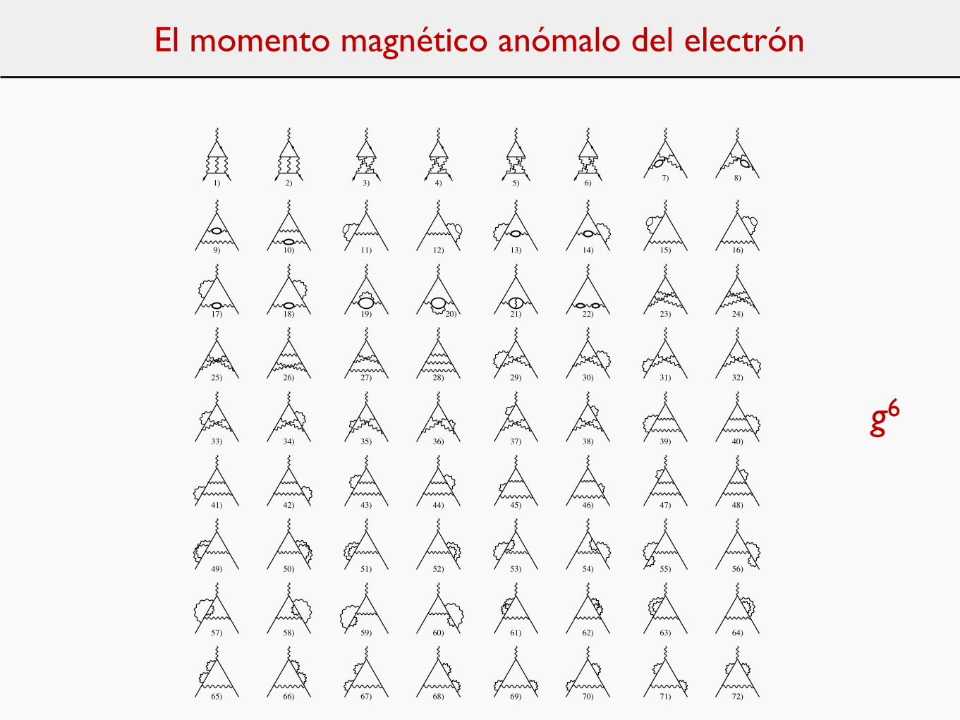
El momento magnético anómalo del electrón
1) 2) 3) 4) 5) 6) 7) 8)
9) 10) 11) 12) 13) 14) 15) 16)
17) 18) 19) 20) 21) 22) 23) 24)
25) 26) 27) 28) 29) 30) 31) 32)
33) 34) 35) 36) 37) 38) 39) 40)
41) 42) 43) 44) 45) 46) 47) 48)
49) 50) 51) 52) 53) 54) 55) 56)
57) 58) 59) 60) 61) 62) 63) 64)
65) 66) 67) 68) 69) 70) 71) 72)
Fig. 10. The universal third order contribution to aµ. All fermion loops here are muon–loops. Graphs 1) to 6) are the light–by—light scattering diagrams. Graphs 7) to 22) include photon vacuum polarization insertions. All non–universal contributions followby replacing at least one muon in a closed loop by some other fermion.
set of diagrams Fig. 12. The latter 518 diagrams without fermion loops also are responsible for the largestpart of the uncertainty in Eq. (52). Note that the universal O(!4) contribution is sizable, about 6 standarddeviations at current experimental accuracy, and a precise knowledge of this term is absolutely crucial forthe comparison between theory and experiment.• The universal 5–loop QED contribution is still largely unknown. Using the recipe proposed in Ref. [37],one obtains the following bound
A(10)1 = 0.0(4.6) , (53)
for the universal part as an estimate for the missing higher order terms.As a result the universal QED contribution may be written as
auni! = 0.5
!!
"
"
! 0.328 478 965 579 193 78 . . .!!
"
"2
+1.181 241 456 587 . . .!!
"
"3! 1.9144(35)
!!
"
"4+ 0.0(4.6)
!!
"
"5
23
g6
1) 2) 3) 4) 5) 6) 7) 8)
9) 10) 11) 12) 13) 14) 15) 16)
17) 18) 19) 20) 21) 22) 23) 24)
25) 26) 27) 28) 29) 30) 31) 32)
33) 34) 35) 36) 37) 38) 39) 40)
41) 42) 43) 44) 45) 46) 47) 48)
49) 50) 51) 52) 53) 54) 55) 56)
57) 58) 59) 60) 61) 62) 63) 64)
65) 66) 67) 68) 69) 70) 71) 72)
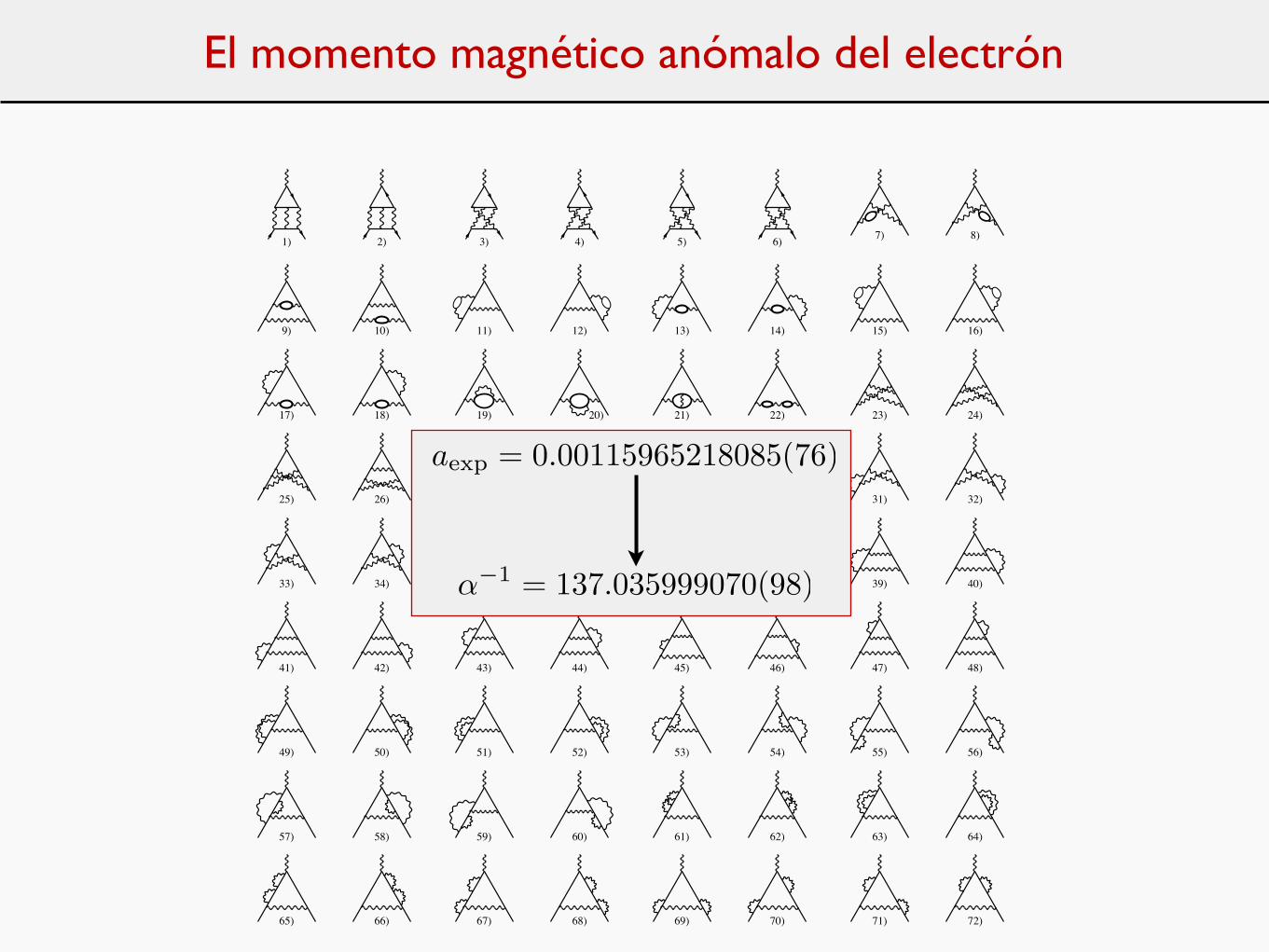
El momento magnético anómalo del electrón
aexp = 0.00115965218085(76)
α−1 = 137.035999070(98)
La edad de plata de la teoría de campos
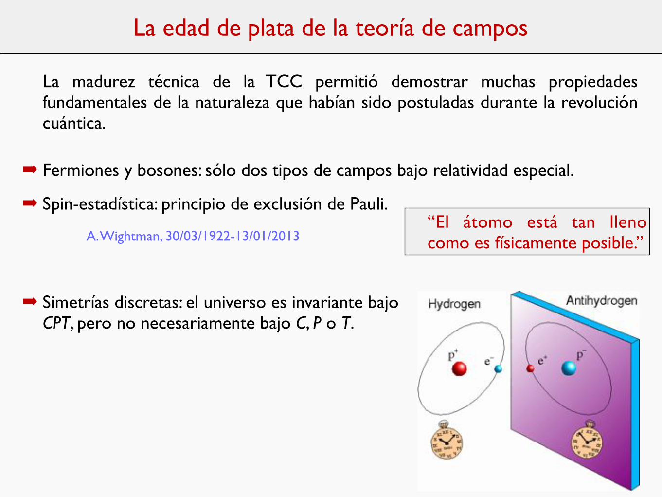
La madurez técnica de la TCC permitió demostrar muchas propiedades fundamentales de la naturaleza que habían sido postuladas durante la revolución cuántica.
! Fermiones y bosones: sólo dos tipos de campos bajo relatividad especial.
! Spin-estadística: principio de exclusión de Pauli.
! Simetrías discretas: el universo es invariante bajo CPT, pero no necesariamente bajo C, P o T.
“El átomo está tan lleno como es físicamente posible.”A. Wightman, 30/03/1922-13/01/2013
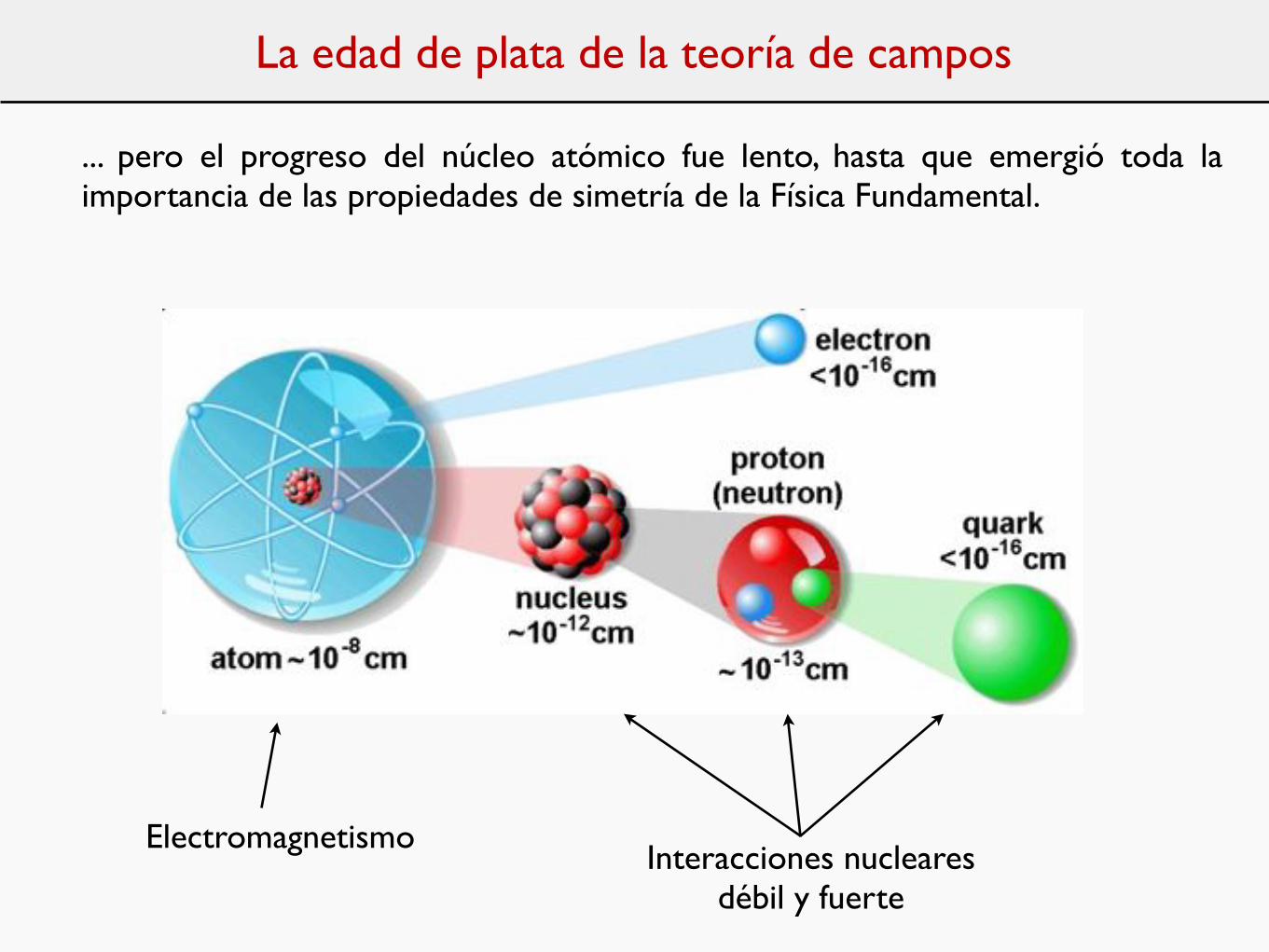
... pero el progreso del núcleo atómico fue lento, hasta que emergió toda la importancia de las propiedades de simetría de la Física Fundamental.
ElectromagnetismoInteracciones nucleares
débil y fuerte
La edad de plata de la teoría de campos
Simetría: La edad de oro de la teoría de campos
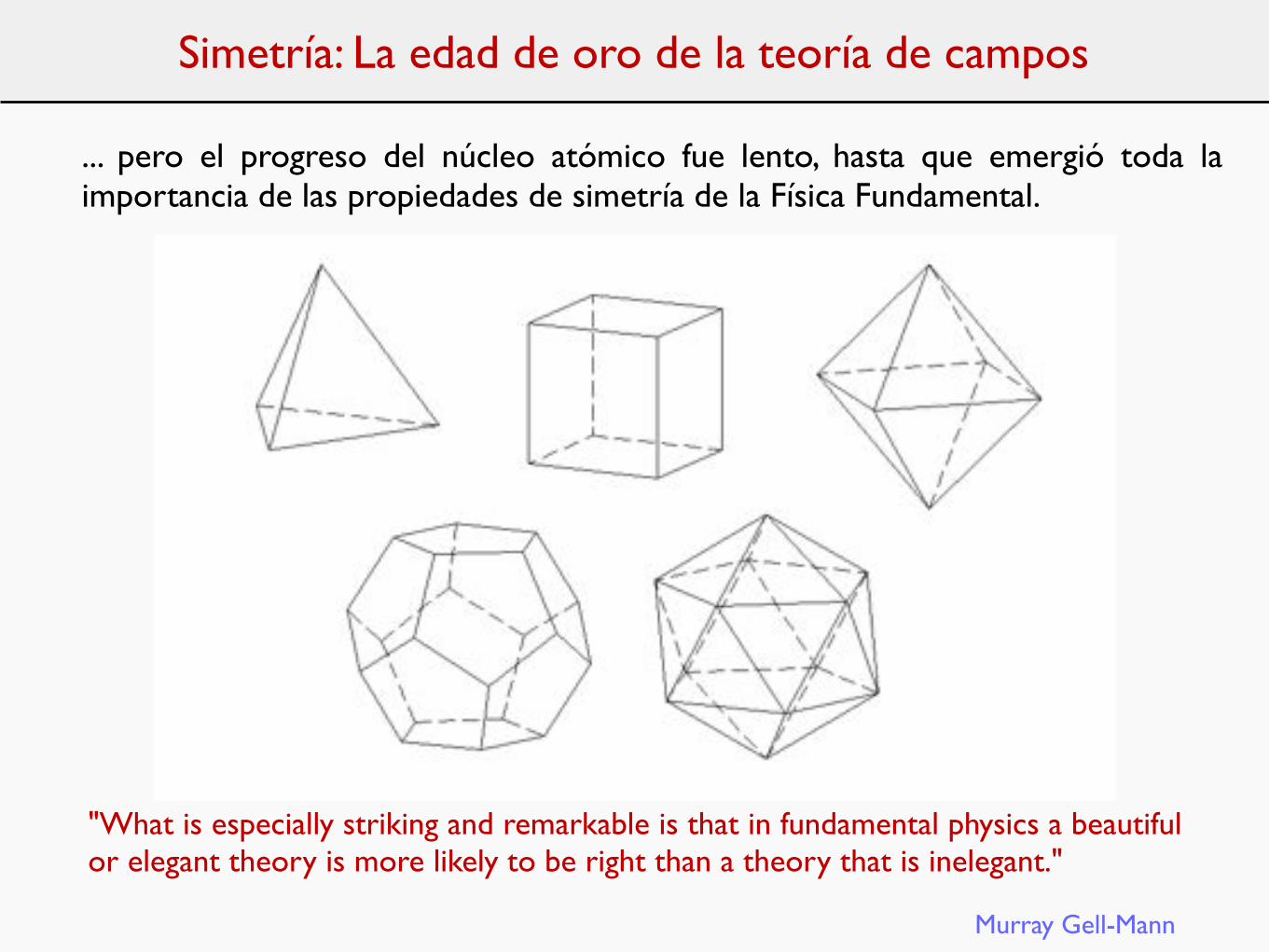
... pero el progreso del núcleo atómico fue lento, hasta que emergió toda la importancia de las propiedades de simetría de la Física Fundamental.
"What is especially striking and remarkable is that in fundamental physics a beautiful or elegant theory is more likely to be right than a theory that is inelegant."
Murray Gell-Mann
Plan
Introducción: escalas de espacio y de energía en Física Fundamental.
Física Cuántica y Relatividad Especial.
Las preguntas revolucionarias.
Dirac y la Mecánica Cuántica Relativista.
Las interacciones nucleares débil y fuerte: neutrinos y mesones.
Interludio: diagramas de Feynman.
Teoría Cuántica de Campos.
Efectos cuánticos y fuerzas fundamentales.
Infinitos y Guerras.
La Edad de Plata: Electrodinámica Cuántica y leyes fundamentales.
Simetrías: la Edad de Oro.
El Camino Óctuple: Quarks.
La interacción electrodébil: corrientes neutras.
Más infinitos.
El Modelo Estándar de la Física de Partículas.
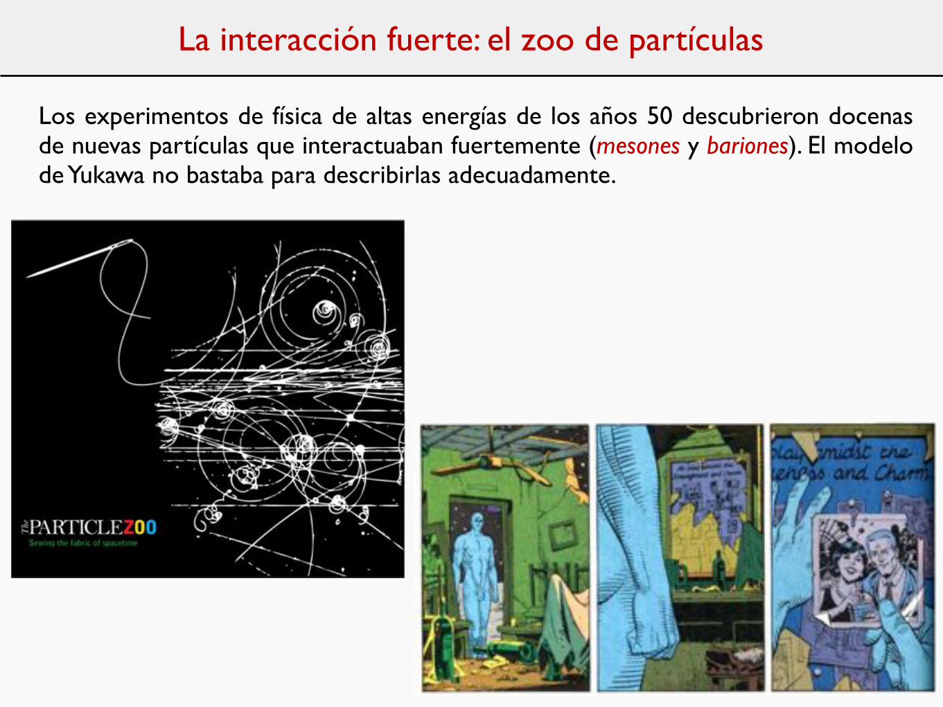
La interacción fuerte: el zoo de partículas
Los experimentos de física de altas energías de los años 50 descubrieron docenas de nuevas partículas que interactuaban fuertemente (mesones y bariones). El modelo de Yukawa no bastaba para describirlas adecuadamente.
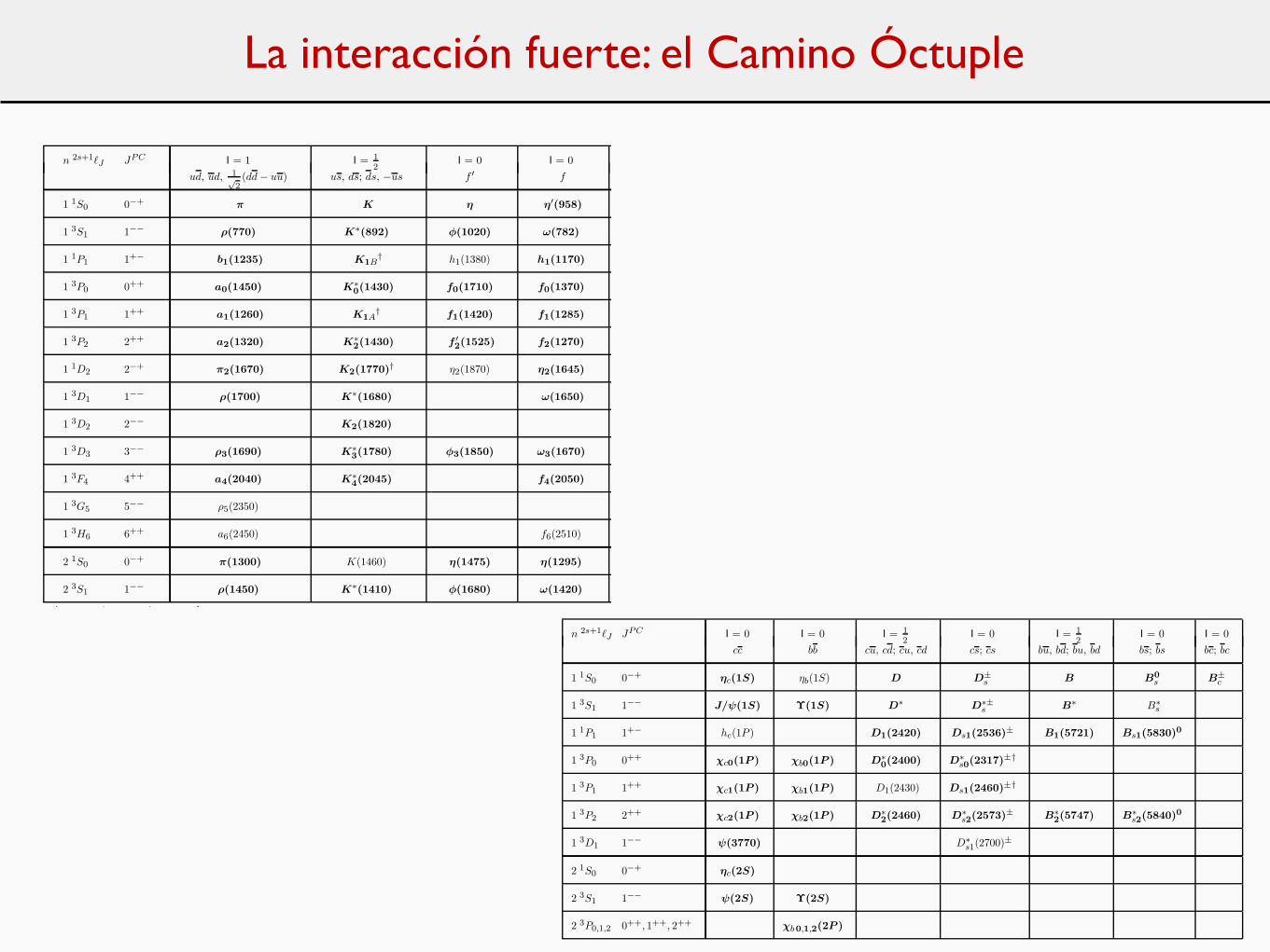
La interacción fuerte: el Camino Óctuple
inicio de la edad de oro de la física teórica de partículas
La interacción fuerte: el Camino Óctuple
14. Quark model 5
Table 14.2: Suggested qq quark-model assignments for some of the observed light mesons. Mesons in bold face are included in the MesonSummary Table. The wave functions f and f ! are given in the text. The singlet-octet mixing angles from the quadratic and linear massformulae are also given for the well established nonets. The classification of the 0++ mesons is tentative and the mixing angle uncertaindue to large uncertainties in some of the masses. Also, the f0(1710) and f0(1370) are expected to mix with the f0(1500). The latter isnot in this table as it is hard to accommodate in the scalar nonet. The light scalars a0(980), f0(980), and f0(600) are often considered asmeson-meson resonances or four-quark states, and are therefore not included in the table. See the “Note on Scalar Mesons” in the MesonListings for details and alternative schemes.
n 2s+1!J JPC I = 1 I = 12
I = 0 I = 0 "quad "lin
ud, ud, 1"2(dd ! uu) us, ds; ds, !us f ! f [#] [#]
1 1S0 0$+ ! K " "!(958) !11.5 !24.6
1 3S1 1$$ #(770) K%(892) $(1020) %(782) 38.7 36.0
1 1P1 1+$ b1(1235) K1B† h1(1380) h1(1170)
1 3P0 0++ a0(1450) K%0(1430) f0(1710) f0(1370)
1 3P1 1++ a1(1260) K1A† f1(1420) f1(1285)
1 3P2 2++ a2(1320) K%2(1430) f !
2(1525) f2(1270) 29.6 28.0
1 1D2 2$+ !2(1670) K2(1770)† #2(1870) "2(1645)
1 3D1 1$$ #(1700) K%(1680) %(1650)
1 3D2 2$$ K2(1820)
1 3D3 3$$ #3(1690) K%3(1780) $3(1850) %3(1670) 32.0 31.0
1 3F4 4++ a4(2040) K%4(2045) f4(2050)
1 3G5 5$$ $5(2350)
1 3H6 6++ a6(2450) f6(2510)
2 1S0 0$+ !(1300) K(1460) "(1475) "(1295)
2 3S1 1$$ #(1450) K%(1410) $(1680) %(1420)
† The 1+± and 2$± isospin 12
states mix. In particular, the K1A and K1B are nearly equal (45#) mixtures of the K1(1270) and K1(1400).The physical vector mesons listed under 13D1 and 23S1 may be mixtures of 13D1 and 23S1, or even have hybrid components.
July 30, 2010 14:36
6 14. Quark model
Table 14.3: qq quark-model assignments for the observed heavy mesons. Mesons in bold face are included in the Meson Summary Table.
n 2s+1!J JPC I = 0 I = 0 I = 12
I = 0 I = 12
I = 0 I = 0cc bb cu, cd; cu, cd cs; cs bu, bd; bu, bd bs; bs bc; bc
1 1S0 0!+ !c(1S) "b(1S) D D±s B B0
s B±c
1 3S1 1!! J/"(1S) !(1S) D" D"±s B" B"
s
1 1P1 1+! hc(1P ) D1(2420) Ds1(2536)± B1(5721) Bs1(5830)0
1 3P0 0++ #c0(1P ) #b0(1P ) D"0(2400) D"
s0(2317)±†
1 3P1 1++ #c1(1P ) #b1(1P ) D1(2430) Ds1(2460)±†
1 3P2 2++ #c2(1P ) #b2(1P ) D"2(2460) D"
s2(2573)± B"
2(5747) B"s2(5840)
0
1 3D1 1!! "(3770) D"s1(2700)
±
2 1S0 0!+ !c(2S)
2 3S1 1!! "(2S) !(2S)
2 3P0,1,2 0++, 1++, 2++ #b0,1,2(2P )
† The masses of these states are considerably smaller than most theoretical predictions. They have also been considered as four-quark states(See the “Note on Non-qq Mesons” at the end of the Meson Listings). The open flavor states in the 1+! and 1++ rows are mixtures of the1+± states.
July 30, 2010 14:36
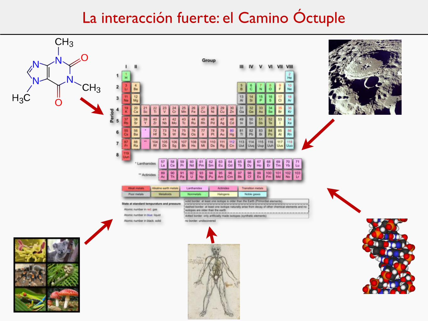
La interacción fuerte: el Camino Óctuple
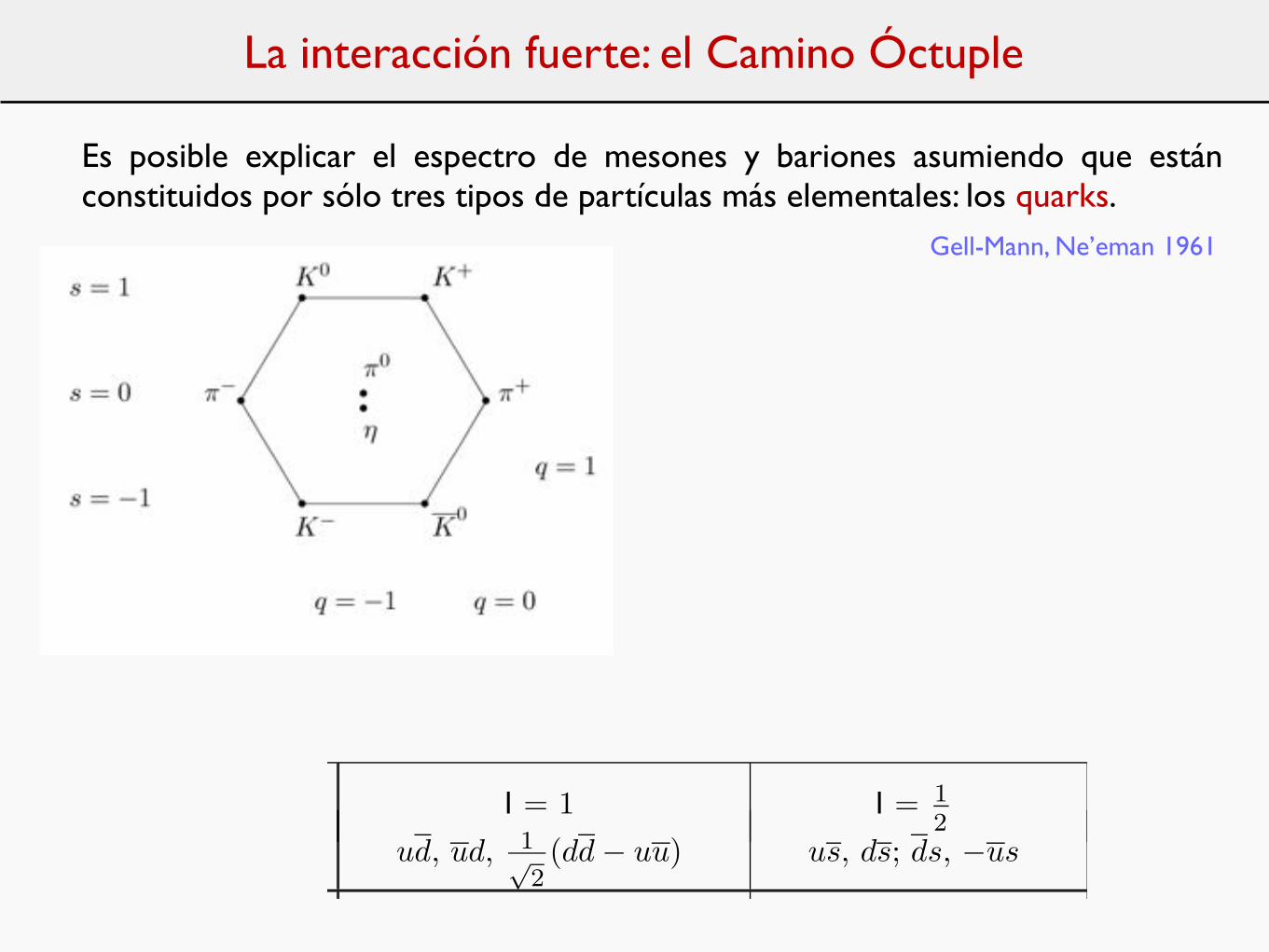
Es posible explicar el espectro de mesones y bariones asumiendo que están constituidos por sólo tres tipos de partículas más elementales: los quarks.
Gell-Mann, Ne’eman 1961
La interacción fuerte: el Camino Óctuple
14. Quark model 5
Table 14.2: Suggested qq quark-model assignments for some of the observed light mesons. Mesons in bold face are included in the MesonSummary Table. The wave functions f and f ! are given in the text. The singlet-octet mixing angles from the quadratic and linear massformulae are also given for the well established nonets. The classification of the 0++ mesons is tentative and the mixing angle uncertaindue to large uncertainties in some of the masses. Also, the f0(1710) and f0(1370) are expected to mix with the f0(1500). The latter isnot in this table as it is hard to accommodate in the scalar nonet. The light scalars a0(980), f0(980), and f0(600) are often considered asmeson-meson resonances or four-quark states, and are therefore not included in the table. See the “Note on Scalar Mesons” in the MesonListings for details and alternative schemes.
n 2s+1!J JPC I = 1 I = 12
I = 0 I = 0 "quad "lin
ud, ud, 1"2(dd ! uu) us, ds; ds, !us f ! f [#] [#]
1 1S0 0$+ ! K " "!(958) !11.5 !24.6
1 3S1 1$$ #(770) K%(892) $(1020) %(782) 38.7 36.0
1 1P1 1+$ b1(1235) K1B† h1(1380) h1(1170)
1 3P0 0++ a0(1450) K%0(1430) f0(1710) f0(1370)
1 3P1 1++ a1(1260) K1A† f1(1420) f1(1285)
1 3P2 2++ a2(1320) K%2(1430) f !
2(1525) f2(1270) 29.6 28.0
1 1D2 2$+ !2(1670) K2(1770)† #2(1870) "2(1645)
1 3D1 1$$ #(1700) K%(1680) %(1650)
1 3D2 2$$ K2(1820)
1 3D3 3$$ #3(1690) K%3(1780) $3(1850) %3(1670) 32.0 31.0
1 3F4 4++ a4(2040) K%4(2045) f4(2050)
1 3G5 5$$ $5(2350)
1 3H6 6++ a6(2450) f6(2510)
2 1S0 0$+ !(1300) K(1460) "(1475) "(1295)
2 3S1 1$$ #(1450) K%(1410) $(1680) %(1420)
† The 1+± and 2$± isospin 12
states mix. In particular, the K1A and K1B are nearly equal (45#) mixtures of the K1(1270) and K1(1400).The physical vector mesons listed under 13D1 and 23S1 may be mixtures of 13D1 and 23S1, or even have hybrid components.
July 30, 2010 14:36
Es posible explicar el espectro de mesones y bariones asumiendo que están constituidos por sólo tres tipos de partículas más elementales: los quarks.
Gell-Mann, Ne’eman 1961
Simetr
ía SU
(3) (
“de s
abor
”)
La interacción fuerte: el Camino Óctuple
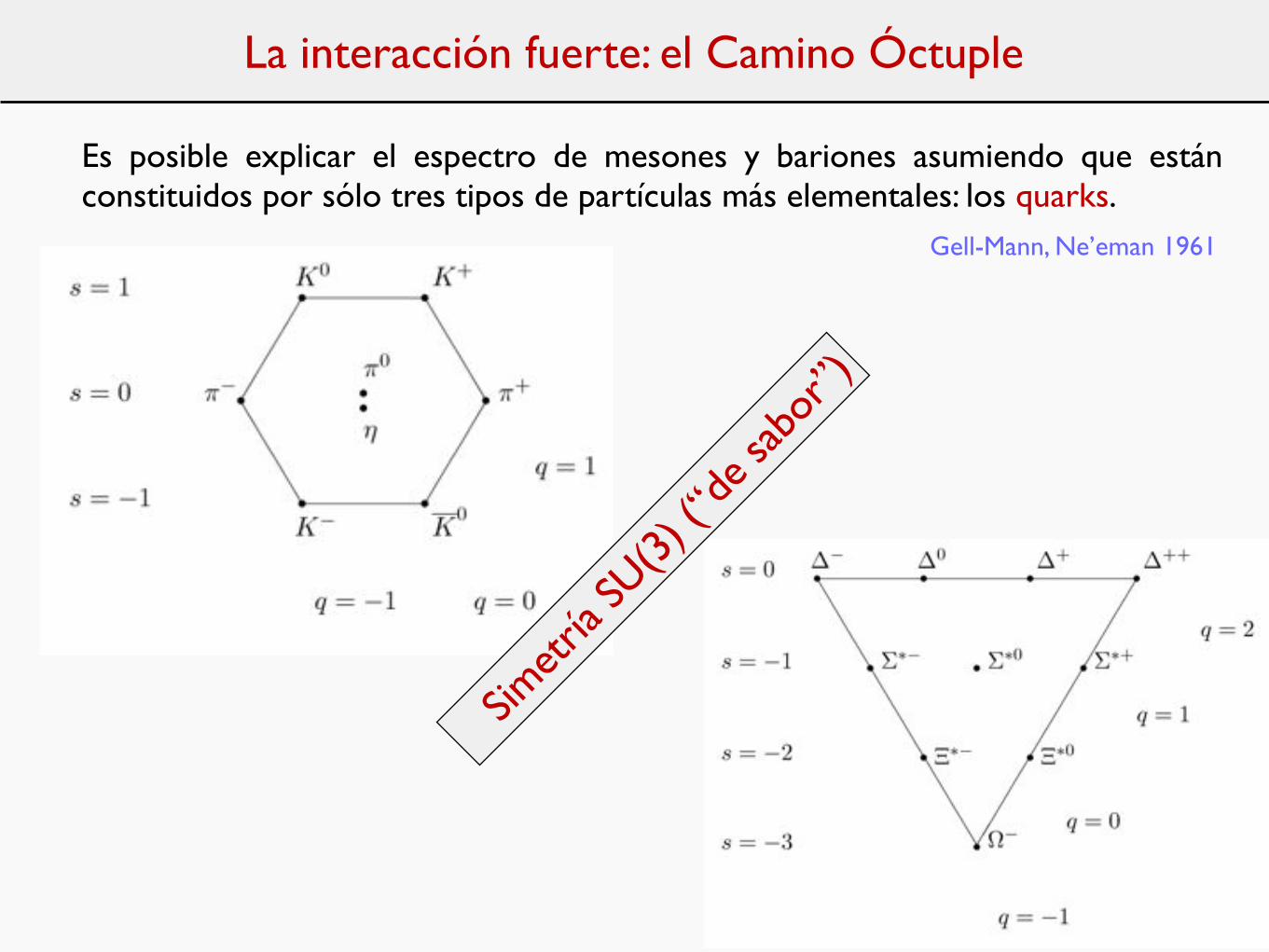
Es posible explicar el espectro de mesones y bariones asumiendo que están constituidos por sólo tres tipos de partículas más elementales: los quarks.
Gell-Mann, Ne’eman 1961
Principio de exclusión de Pauli: tres fermiones idénticos no pueden estar en el mismo estado.
La interacción fuerte: el Camino Óctuple
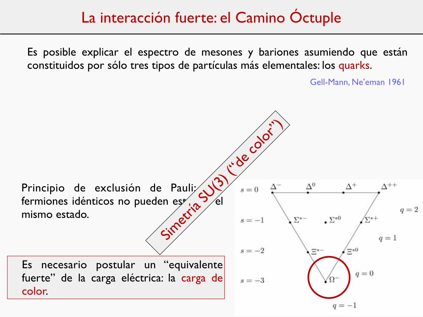
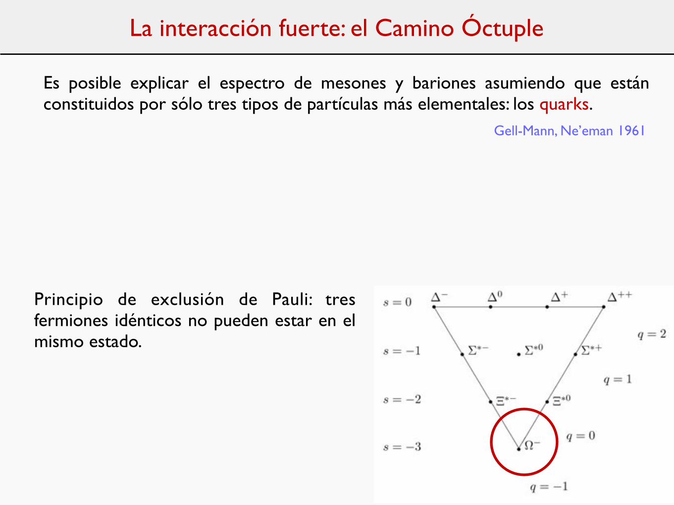
Es posible explicar el espectro de mesones y bariones asumiendo que están constituidos por sólo tres tipos de partículas más elementales: los quarks.
Gell-Mann, Ne’eman 1961
Principio de exclusión de Pauli: tres fermiones idénticos no pueden estar en el mismo estado.
Es necesario postular un “equivalente fuerte” de la carga eléctrica: la carga de color.
La interacción fuerte: el Camino Óctuple
Simetr
ía SU
(3) (
“de c
olor”
)
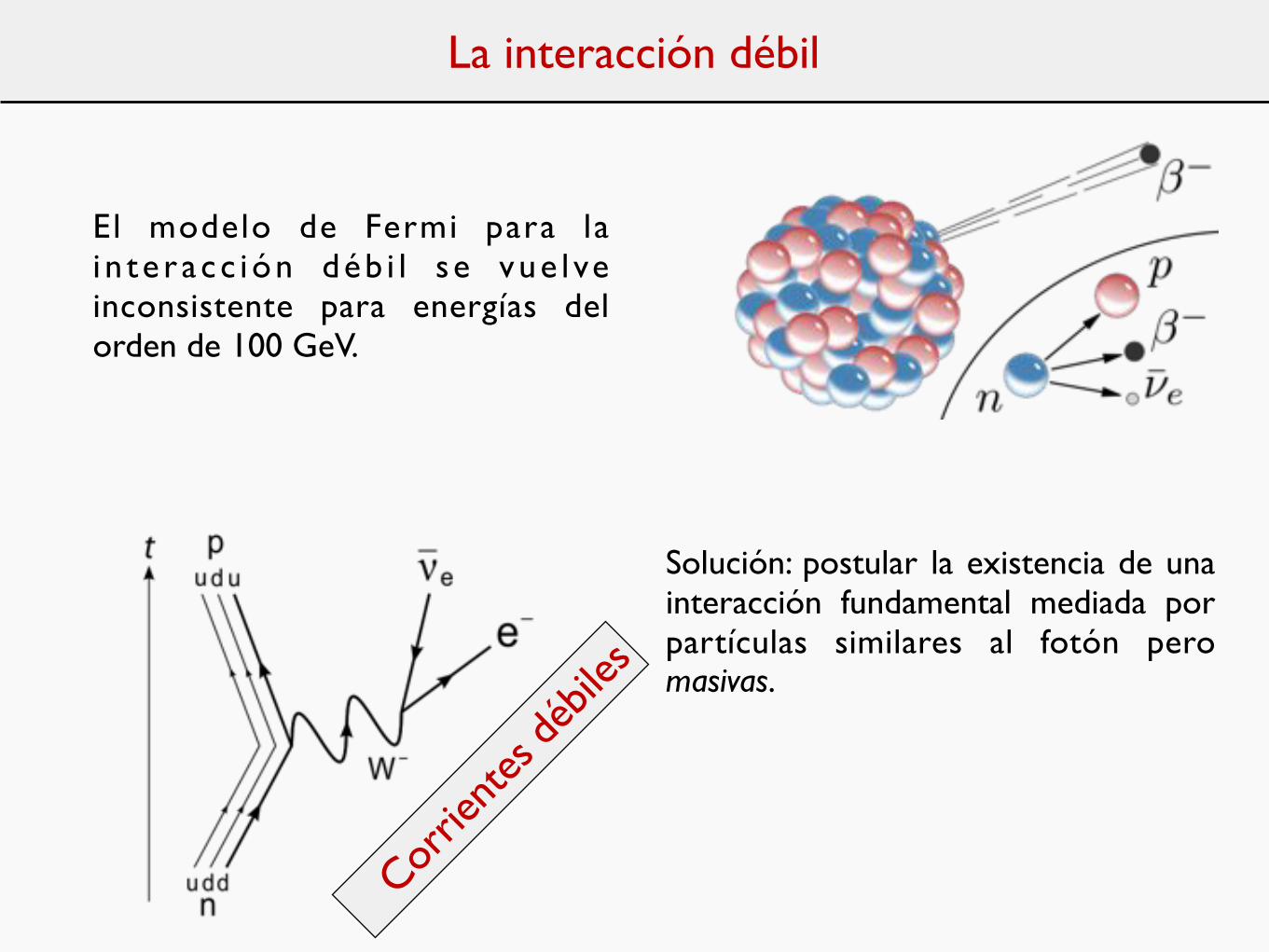
La interacción débil
El modelo de Fermi para la i n t e r acc ión déb i l s e vue l ve inconsistente para energías del orden de 100 GeV.
Solución: postular la existencia de una interacción fundamental mediada por partículas similares al fotón pero masivas.
Corrie
ntes
débil
es
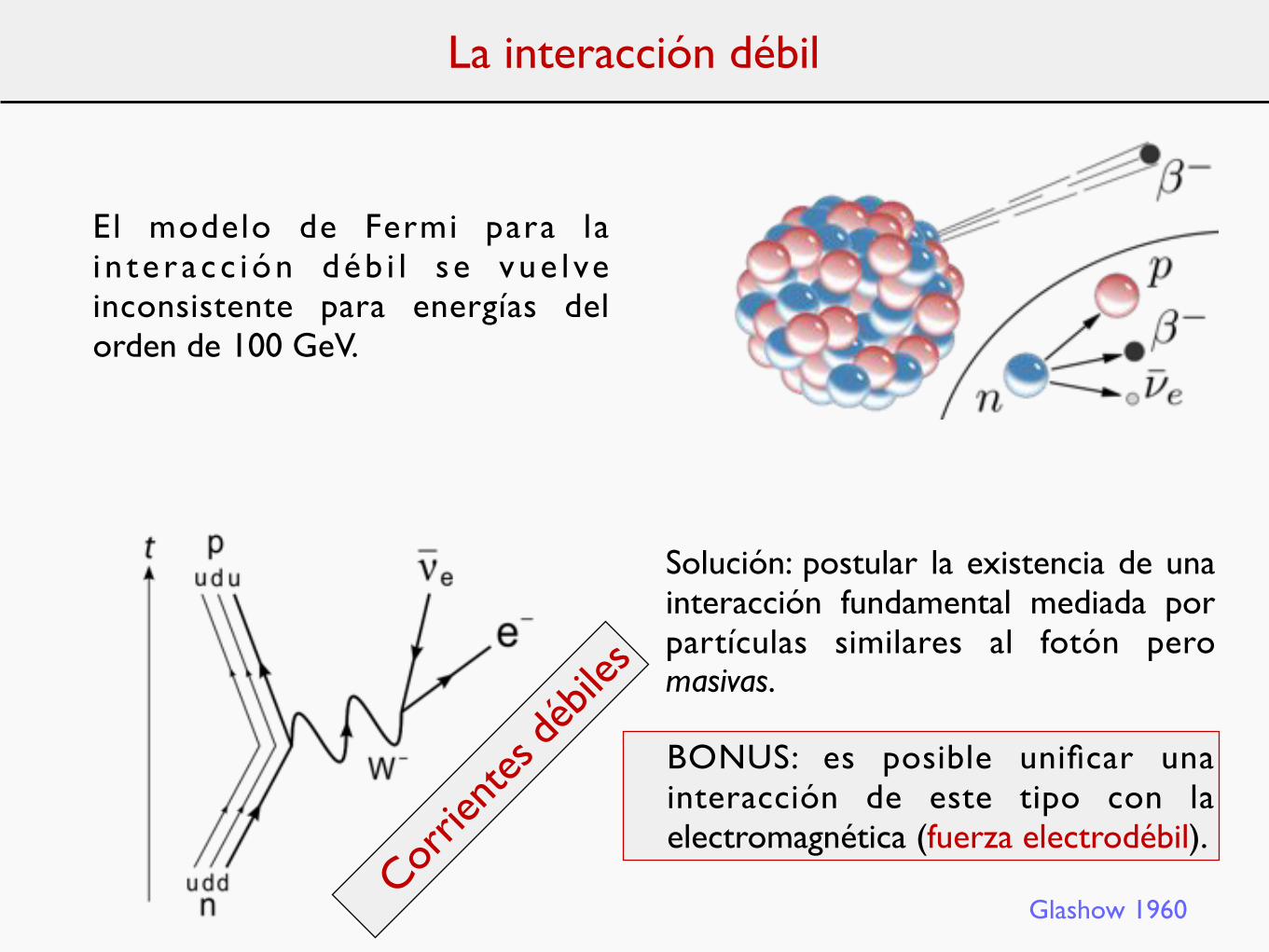
La interacción débil
Solución: postular la existencia de una interacción fundamental mediada por partículas similares al fotón pero masivas.
BONUS: es posible unificar una interacción de este tipo con la electromagnética (fuerza electrodébil).
Glashow 1960
El modelo de Fermi para la i n t e r acc ión déb i l s e vue l ve inconsistente para energías del orden de 100 GeV.
Corrie
ntes
débil
es
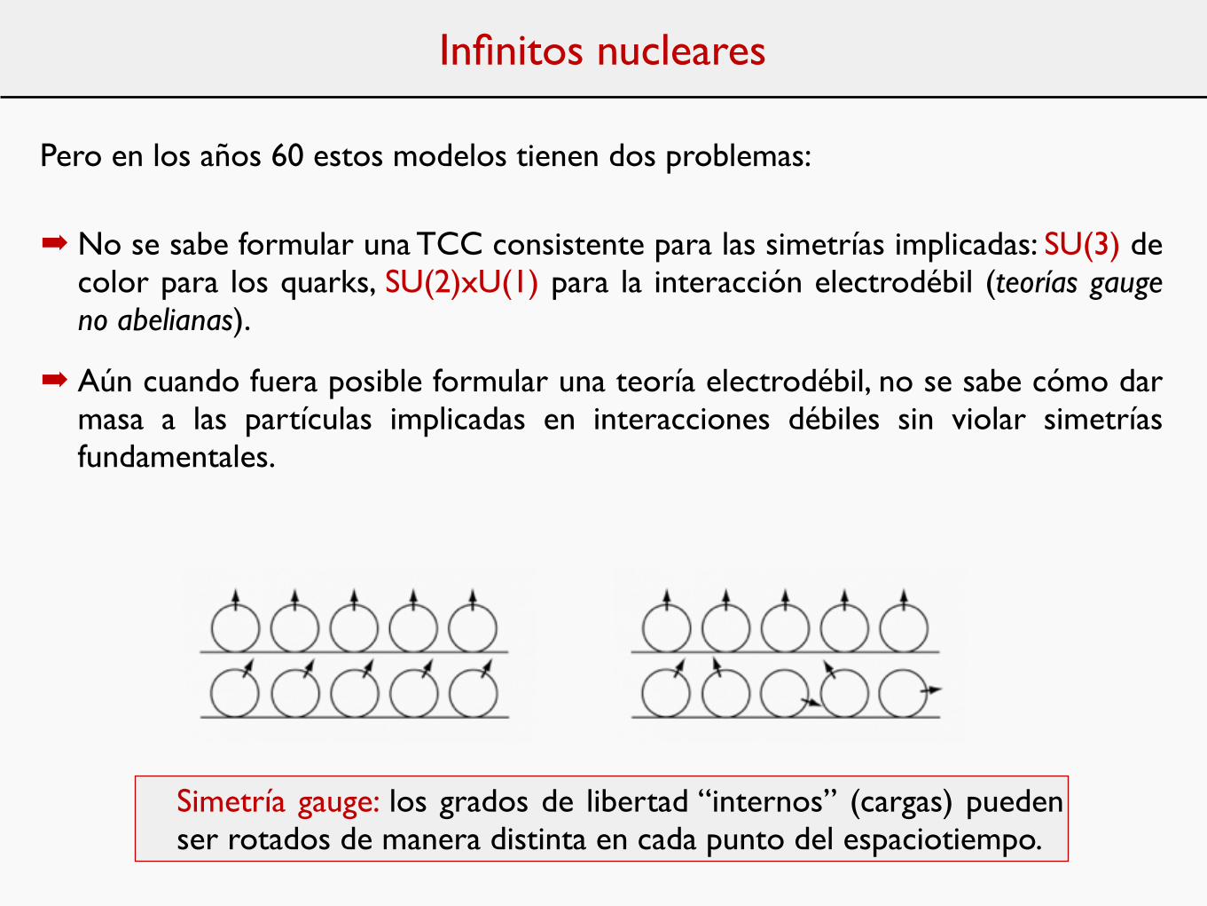
Infinitos nucleares
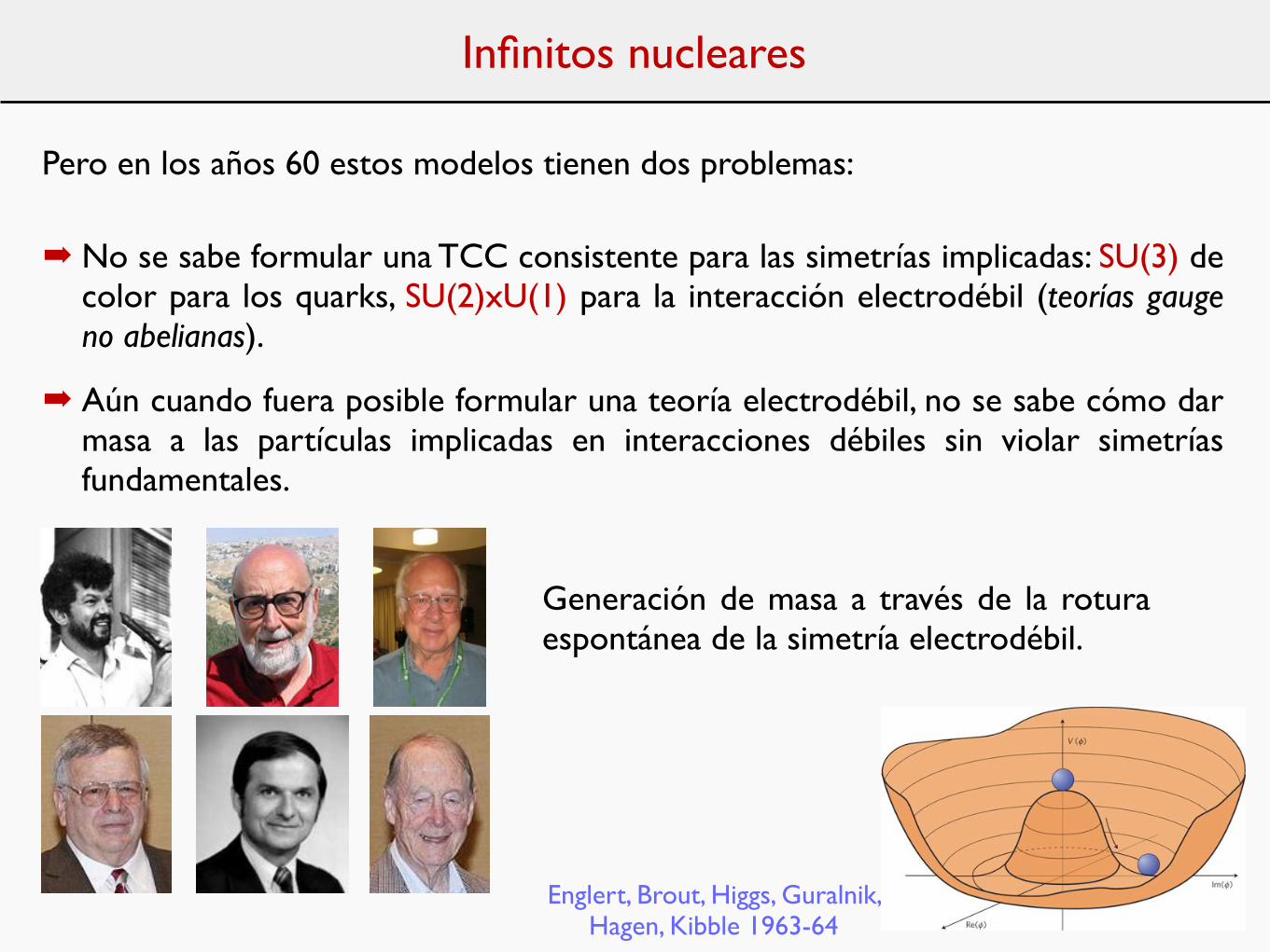
Pero en los años 60 estos modelos tienen dos problemas:
! No se sabe formular una TCC consistente para las simetrías implicadas: SU(3) de color para los quarks, SU(2)xU(1) para la interacción electrodébil (teorías gauge no abelianas).
! Aún cuando fuera posible formular una teoría electrodébil, no se sabe cómo dar masa a las partículas implicadas en interacciones débiles sin violar simetrías fundamentales.
Simetría gauge: los grados de libertad “internos” (cargas) pueden ser rotados de manera distinta en cada punto del espaciotiempo.
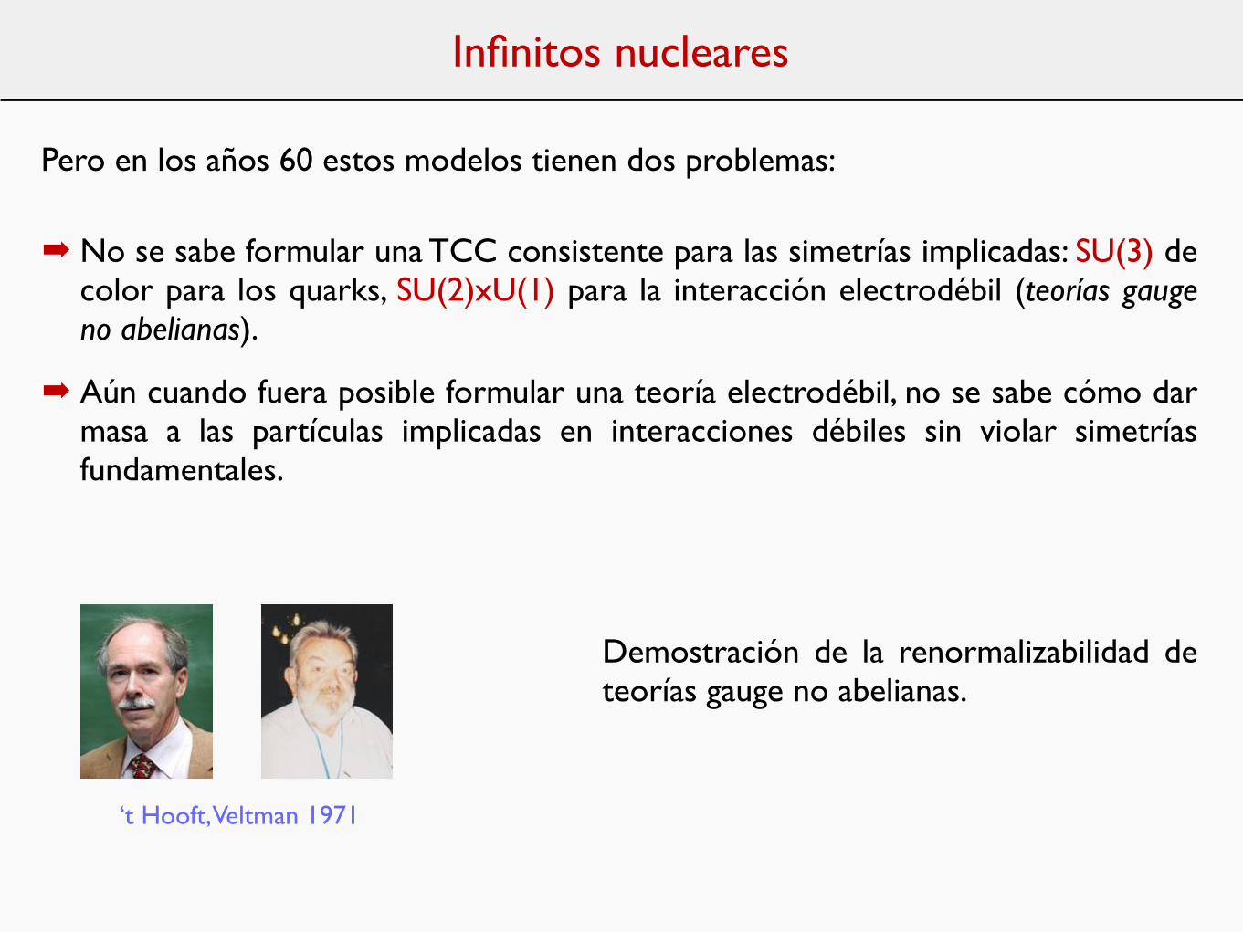
Infinitos nucleares
Demostración de la renormalizabilidad de teorías gauge no abelianas.
‘t Hooft, Veltman 1971
! No se sabe formular una TCC consistente para las simetrías implicadas: SU(3) de color para los quarks, SU(2)xU(1) para la interacción electrodébil (teorías gauge no abelianas).
! Aún cuando fuera posible formular una teoría electrodébil, no se sabe cómo dar masa a las partículas implicadas en interacciones débiles sin violar simetrías fundamentales.
Pero en los años 60 estos modelos tienen dos problemas:
Infinitos nucleares
Generación de masa a través de la rotura espontánea de la simetría electrodébil.
Englert, Brout, Higgs, Guralnik, Hagen, Kibble 1963-64
! No se sabe formular una TCC consistente para las simetrías implicadas: SU(3) de color para los quarks, SU(2)xU(1) para la interacción electrodébil (teorías gauge no abelianas).
! Aún cuando fuera posible formular una teoría electrodébil, no se sabe cómo dar masa a las partículas implicadas en interacciones débiles sin violar simetrías fundamentales.
Pero en los años 60 estos modelos tienen dos problemas:
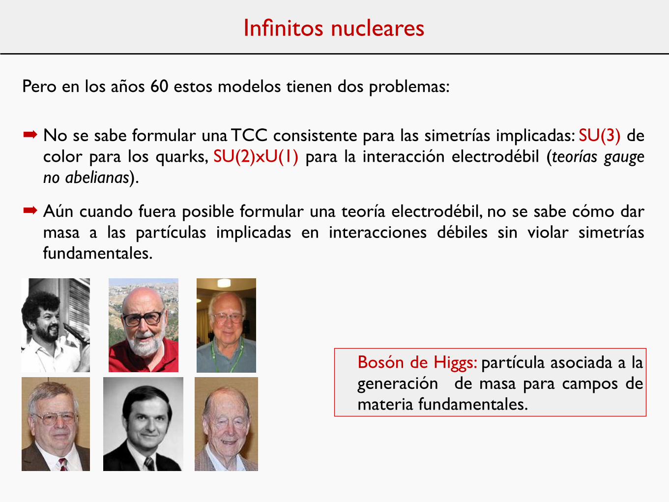
Bosón de Higgs: partícula asociada a la generación de masa para campos de materia fundamentales.
Infinitos nucleares
! No se sabe formular una TCC consistente para las simetrías implicadas: SU(3) de color para los quarks, SU(2)xU(1) para la interacción electrodébil (teorías gauge no abelianas).
! Aún cuando fuera posible formular una teoría electrodébil, no se sabe cómo dar masa a las partículas implicadas en interacciones débiles sin violar simetrías fundamentales.
Pero en los años 60 estos modelos tienen dos problemas:
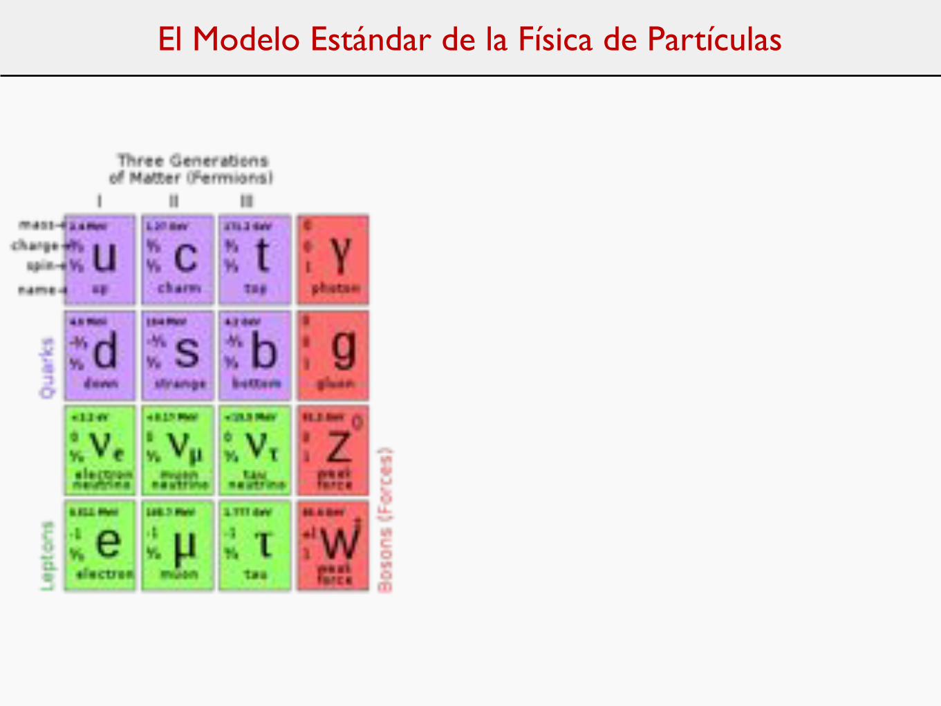
El Modelo Estándar de la Física de Partículas
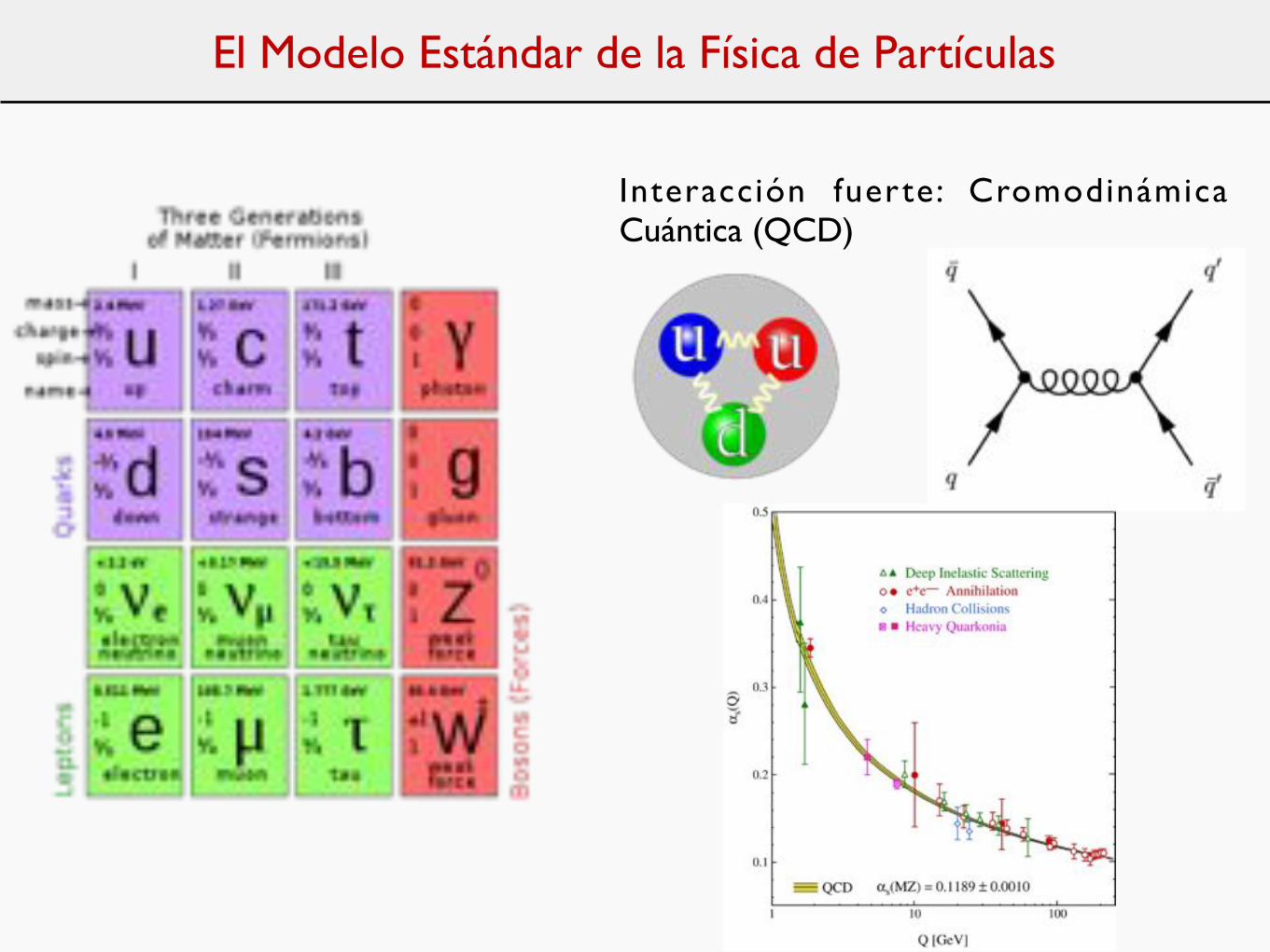
El Modelo Estándar de la Física de Partículas
Interacción fuerte: Cromodinámica Cuántica (QCD)
El Modelo Estándar de la Física de Partículas
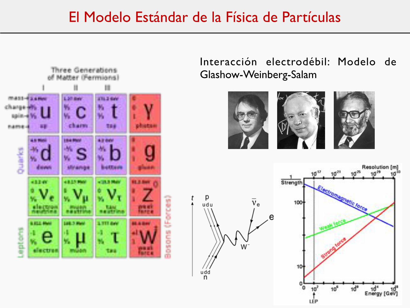
Interacción electrodébil: Modelo de Glashow-Weinberg-Salam
El Modelo Estándar de la Física de Partículas
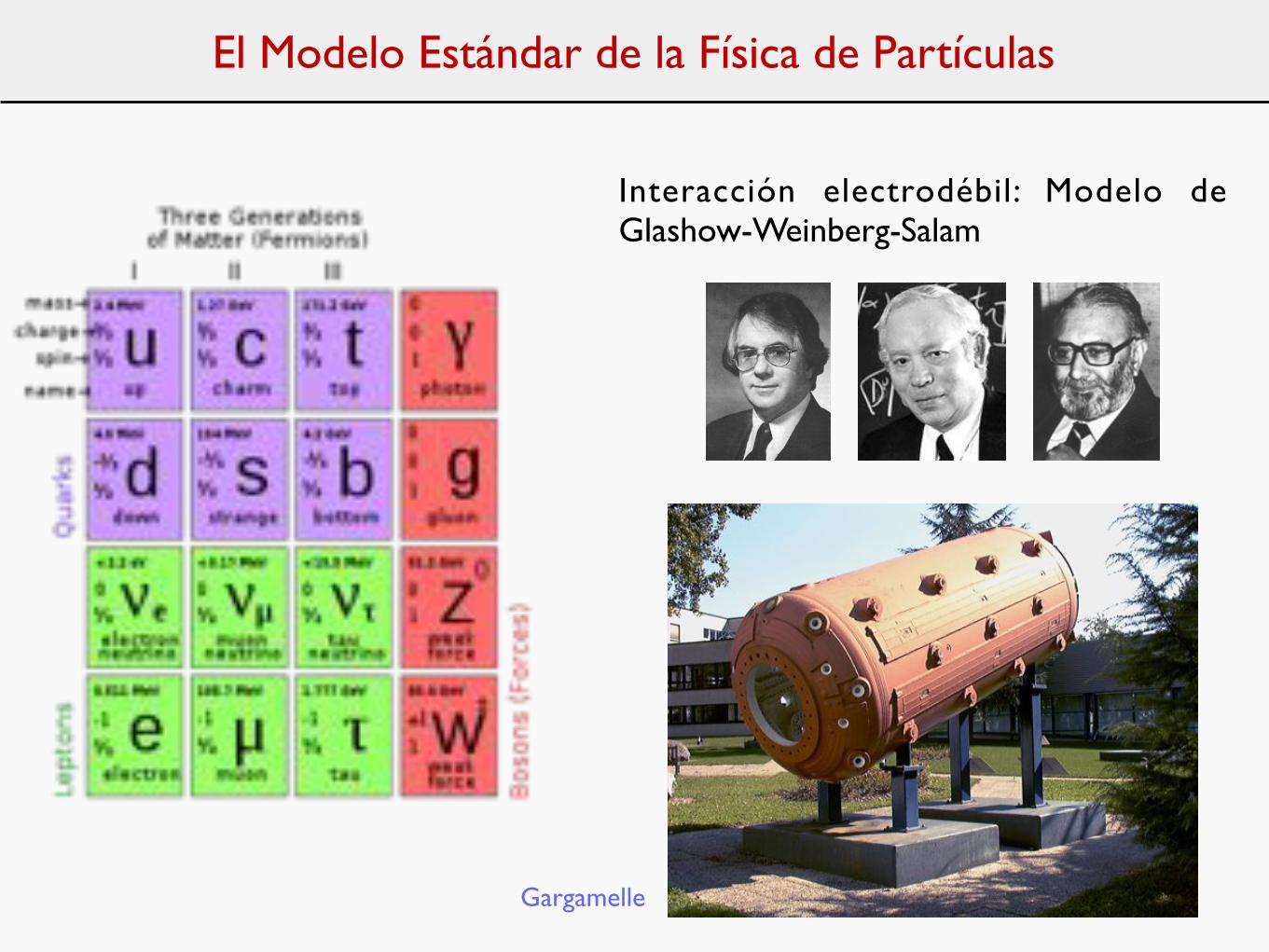
Interacción electrodébil: Modelo de Glashow-Weinberg-Salam
Gargamelle
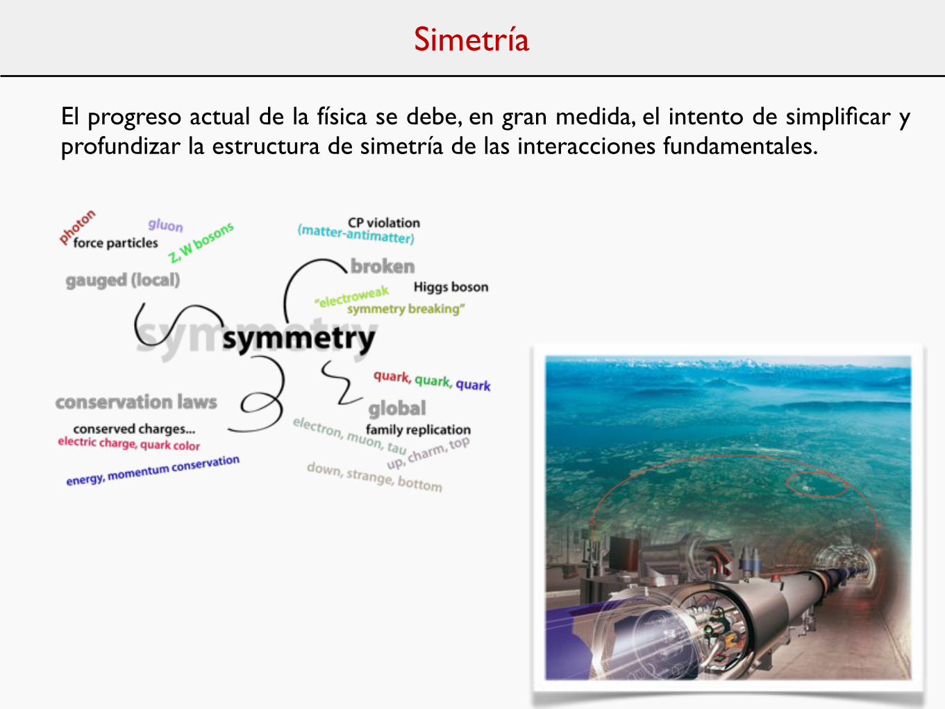
Simetría
El progreso actual de la física se debe, en gran medida, el intento de simplificar y profundizar la estructura de simetría de las interacciones fundamentales.