criptograf a en campos nitos de caracter stica...
TRANSCRIPT
Centro de Investigacion y de EstudiosAvanzados del Instituto Politecnico Nacional
Unidad Zacatenco
Departamento de Computacion
Criptografıa en campos finitos de caracterıstica
chica
Tesis que presenta
Thomaz Eduardo de Figueiredo Oliveira
para obtener el Grado de
Doctor en Ciencias en Computacion
Directores de tesis:
Dr. Francisco Jose Rambo Rodrıguez Henrıquez
Dr. Julio Cesar Lopez Hernandez
Ciudad de Mexico Febrero 2016

Acknowledgements
I would like to thank my advisor and co-advisor, professors Francisco RodrıguezHenrıquez and Julio Lopez who guided me through the amazing area of cryptogra-phy. I also thank professor Alfred Menezes for his warm reception during my stayWaterloo.
A special thanks to my thesis reviewers who provided me valuable comments andsuggestions.
I also thank my friends from the cryptography lab for sharing their knowledge inall these years. A special thanks to the department staff who supported me duringmy Ph. D studies.
I thank the Consejo Nacional de Ciencia y Tecnologia - CONACyT (projectnumber 180421) for their financial support during my stay in Mexico and Canada.Also, a special thanks to ABACUS-Cinvestav for providing us computing resourceswhich were essential for concluding our projects.
A todos mis amigos de Mexico que compartieron momentos inolvidables.
E finalmente, um agradecimento especial a minha famılia. Sem o seu apoio,minha experiencia durante estes quatro anos seria muito mais difıcil.
iii

iv ACKNOWLEDGEMENTS
Abstract
Since the beginning of public-key cryptography, small-characteristic finite fields havebeen proposed as basic mathematical structures for implementing electronic com-munication protocols and standardized algorithms that achieve different informationsecurity objectives. This is because the arithmetic on these fields can be efficientlyrealized in the binary and trinary number systems, which are fundamental in mod-ern computer architectures. This thesis proposes a concrete analysis of the currentsecurity and performance of different primitives based on these fields.
In the first part of this document, we introduce efficient software implementa-tions of the point multiplication algorithm for two families of binary elliptic curveswhich are provided with efficiently computable endomorphisms. The first class iscalled Galbraith-Lin-Scott (GLS) curves. There, we present state-of-the-art imple-mentations based on the Gallant-Lambert-Vanstone decomposition method and onthe Montgomery ladder approach, in order to achieve a high-speed protected andnon-protected code against timing attacks. The second family studied in this thesisis called anomalous binary curves or Koblitz curves. On these elliptic curves, wepresent, for the first time, a timing-attack protected scalar multiplication based onthe regular recoding approach. In addition, we introduce a novel implementationof Koblitz curves defined over the extension field F4, which resulted in an efficientarithmetic that exploits the internal parallelism contained in the newest desktop pro-cessors. All of the previously mentioned implementations are supported by a newprojective coordinate system, denoted lambda-coordinates, which provides state-of-the-art formulas for computing the basic point arithmetic operations.
In the second part, we provide a concrete analysis of the impact of the recent ap-proaches for solving the discrete logarithm problem (DLP) in small-characteristicfields of cryptographic interest. After that, we realize practical attacks againstfields proposed in the literature to realize pairing-based protocols. Finally, we studythe practical implications of the Gaudry-Hess-Smart attack against the binary GLScurves. For that purpose, we analyze and implement techniques to improve the effi-ciency of the Enge-Gaudry algorithm for solving the DLP over hyperelliptic curves.
v

vi ABSTRACT
Resumen
Desde el inicio de la criptografıa de llave publica, los campos finitos de caracterısticachica han sido propuestos como estructuras matematicas en implementacion de pro-tocolos de comunicacion electronica, cuyo objetivo es garantizar distintos atributosde seguridad. Estas estructuras son propuestas porque pueden ser implementadaseficientemente en sistemas numericos binarios o ternarios, los cuales son intrınsecosde las arquitecturas computacionales modernas. En esta tesis se realiza un analisisde la seguridad y eficiencia de distintas primitivas basadas en estos campos finitos.
En la primera parte de la tesis, presentamos la implementacion eficiente en soft-ware del algoritmo para la multiplicacion escalar de puntos en dos familias de curvaselıpticas binarias, las cuales cuentan con endomorfismos eficientemente computables.La primera familia es la llamada de Galbraith-Lin-Scott (GLS). En estas curvaspresentamos implementaciones construidas con los metodos de Gallant-Lambert-Vanstone y la escalera de Montgomery, con la finalidade de computar una multi-plicacion escalar eficiente y protegida contra ataques de canal lateral. La segundafamilia es la denominada como curvas binarias anomalas o curvas de Koblitz. En estafamilia presentamos, de manera inedita, la implementacion del algoritmo de multipli-cacion escalar de puntos protegida contra ataques de canal lateral, basados en tiempo,mediante la tecnica de recodificacion regular. Ademas, introducimos una novedosaimplementacion de las curvas de Koblitz definidas sobre la extension de campo F4,lo que resulto en una aritmetica eficiente que toma vantaja del paralelismo ofrecidopor los procesadores de escritorio mas recientes. Todas las implementaciones men-cionadas fueron basadas en el nuevo sistema de coordinadas proyectivas lambda queaportan formulas al “estado del arte” para el computo de la aritmetica de puntos.
En la segunda parte, realizamos un analisis del impacto de los avances recientesen la solucion del problema del logaritmo discreto (PLD) en campos finitos de car-acterıstica chica de interes criptografico. Tambien, realizamos ataques practicos encampos finitos usados en protocolos basados en emparejamientos. Finalmente, im-plementamos metodos para mejorar la eficiencia del algoritmo de Enge y Gaudrypara resolver el PLD en curvas hiperelipticas.
vii

viii RESUMEN
Resumo
Desde os primordios da criptografia de chave publica, corpos finitos de caracterısticapequena sao propostos como estruturas matematicas para a implementacao de pro-tocolos de comunicacao eletronica que garantem diferentes atributos de segurancada informacao. Estas estruturas sao propostas pois podem ser instanciadas eficiente-mente em sistemas numericos binarios ou ternarios, que sao inerentes nas arquiteturascomputacionais contemporaneas. Esta tese realiza uma analise dos recentes avancosem seguranca e eficiencia em diferentes primitivas baseadas nestes corpos finitos.
Na primeira parte desta tese, descrevemos implementacoes em software de algo-ritmos para a multiplicacao de pontos em duas famılias de curvas elıpticas binariasproporcionadas com endomorfismos eficientemente computaveis. A primeira famıliae chamada curvas Galbraith-Lin-Scott (GLS). Nestas curvas, apresentamos imple-mentacoes baseadas no metodo Gallant-Lambert-Vanstone e na escada de Mont-gomery com a finalidade de gerar uma multiplicacao escalar eficiente e protegidacontra ataques de canal secundario. A segunda famılia denominada curvas binariasanomalas ou curvas de Koblitz. Nesta famılia, realizamos, de maneira inedita, imple-mentacoes do algoritmo de multiplicacao de pontos protegida contra ataques de canalsecundario atraves da tecnica da recodificacao regular. Alem disso, introduzimos im-plementacoes das curvas de Koblitz definidas sobre o corpo de extensao F4, o queresultou em uma aritmetica eficiente e que aproveita o paralelismo interno presentenos processadores desktop. Todas as implementacoes mencionadas sao construıdassobre um novo sistema de coordenadas projetivas denominadas coordenadas lambda,que fornecem formulas de alto nıvel para o calculo da aritmetica de pontos.
Na segunda parte, proporcionamos uma analise dos avancos recentes na resolucaodo problema do logaritmo discreto (PLD) em corpos finitos de caracterıstica pequenadestinados ao uso criptografico. Em seguida, efetuamos ataques praticos em corposfinitos usados em protocolos baseados em emparelhamentos. Finalmente, estudamosas implicacoes praticas do ataque Gaudry-Hess-Smart em curvas binarias GLS. Paratal proposito, implementamos tecnicas para melhorar a eficiencia do algoritmo deEnge e Gaudry para resolver o PLD em curvas hiperelıpticas.
ix

x RESUMO

Resume
Depuis les debuts de la cryptographie asymetrique, les corps finis de petite car-acteristique sont proposes comme structures mathematiques pour les protocoles decommunication electronique, realisant ainsi plusieurs des objectifs de securite. Cesstructures sont proposees parce qu’elles peuvent etre efficacement implementees dansles systemes numeriques binaires ou ternaires, inherents aux architectures informa-tiques contemporaines. Cette these effectue une analyse des progres en securite eten efficacite d’objets mathematiques cryprographiques bases sur ces corps finis.
Dans la premiere partie, nous presentons differentes implementations logicielles ef-ficaces de l’algorithme de multiplication de points sur deux famillies de courbes ellip-tiques binaires possedant des endomorphismes efficacement calculables. La premierecategorie concerne les courbes de Galbraith-Lin-Scott (GLS). Nous presentons desimplementations de multiplication de points basees sur la methode de decompositionGallant-Lambert-Vanstone et sur l’echelle de Montgomery pour developper un coderapide, en version protegee et en version non-protegee contre les attaques par canauxauxiliaires. La deuxieme categorie est composee des courbes de Koblitz. Sur cescourbes, nous presentons pour la premiere fois, un algorithme de multiplication parun scalaire protege contre les attaques par canaux auxiliaires, base sur la methode dela reprogrammation reguliere. De plus, nous introduisons une nouvelle implementationdes courbes de Koblitz definies sur le corps fini F4, qui jouit d’arithmetique efficace ex-ploitant le parallelisme interne des processeurs desktop. Toutes nos implementationssont supportees par un nouveau systeme de coordonnees projectives, coordonneeslambda, qui fournit une representation plus adaptee a l’arithmetique de points.
Dans la deuxieme partie, nous presentons une analyse de l’impact des nouvellesmethodes pour resoudre le probleme du logarithme discret (DLP) dans les corps finisconsideres. En suite, nous procedons a des attaques pratiques contre des corps debase de courbes elliptiques pairing-friendly. Finalement, nous etudions les implica-tions practiques de l’attaque Gaudry-Hess-Smart contre les courbes GLS. Pour cela,nous mettons en œuvre des techniques pour ameliorer l’efficacite de l’algorithme deEnge-Gaudry pour resoudre le DLP dans les courbes hyper-elliptiques.
xi

xii RESUME
Contents
Acknowledgements iii
Abstract v
Resumen vii
Resumo ix
Resume xi
List of Figures xvii
List of Tables xix
List of Algorithms xxi
1 Introduction 11.1 Motivation . . . . . . . . . . . . . . . . . . . . . . . . . . . . . . . . . 21.2 Outline . . . . . . . . . . . . . . . . . . . . . . . . . . . . . . . . . . . 3
I High-Speed Elliptic Curve Cryptography 5
2 Lambda Coordinates 72.1 Coordinate systems . . . . . . . . . . . . . . . . . . . . . . . . . . . . 8
2.1.1 Affine coordinates . . . . . . . . . . . . . . . . . . . . . . . . . 92.1.2 Homogeneous projective coordinates . . . . . . . . . . . . . . 92.1.3 Jacobian projective coordinates . . . . . . . . . . . . . . . . . 102.1.4 Lopez-Dahab projective coordinates . . . . . . . . . . . . . . . 112.1.5 Coordinate systems summary . . . . . . . . . . . . . . . . . . 12
xiii

xiv CONTENTS
2.2 Lambda projective coordinates . . . . . . . . . . . . . . . . . . . . . . 142.2.1 Group law . . . . . . . . . . . . . . . . . . . . . . . . . . . . . 142.2.2 Comparison . . . . . . . . . . . . . . . . . . . . . . . . . . . . 19
2.3 Summary . . . . . . . . . . . . . . . . . . . . . . . . . . . . . . . . . 20
3 Galbraith-Lin-Scott Curves 213.1 Binary field arithmetic . . . . . . . . . . . . . . . . . . . . . . . . . . 22
3.1.1 Field multiplication over Fq . . . . . . . . . . . . . . . . . . . 223.1.2 Field squaring, square root and multi-squaring over Fq . . . . 223.1.3 Field inversion over Fq . . . . . . . . . . . . . . . . . . . . . . 233.1.4 Modular reduction . . . . . . . . . . . . . . . . . . . . . . . . 233.1.5 Half-trace over Fq . . . . . . . . . . . . . . . . . . . . . . . . . 243.1.6 Field arithmetic over Fq2 . . . . . . . . . . . . . . . . . . . . . 25
3.2 GLS binary curves . . . . . . . . . . . . . . . . . . . . . . . . . . . . 263.2.1 Security . . . . . . . . . . . . . . . . . . . . . . . . . . . . . . 27
3.3 GLV scalar multiplication . . . . . . . . . . . . . . . . . . . . . . . . 283.3.1 The GLV method and the w-NAF representation . . . . . . . 283.3.2 Left-to-right double-and-add . . . . . . . . . . . . . . . . . . . 293.3.3 Right-to-left halve-and-add . . . . . . . . . . . . . . . . . . . . 303.3.4 Lambda-coordinates aftermath . . . . . . . . . . . . . . . . . 303.3.5 Parallel scalar multiplication . . . . . . . . . . . . . . . . . . . 333.3.6 Protected scalar multiplication . . . . . . . . . . . . . . . . . . 343.3.7 Results and discussion . . . . . . . . . . . . . . . . . . . . . . 35
3.4 Montgomery ladder scalar multiplication . . . . . . . . . . . . . . . . 423.4.1 Montgomery ladder variants . . . . . . . . . . . . . . . . . . . 433.4.2 Results and discussion . . . . . . . . . . . . . . . . . . . . . . 50
3.5 Summary . . . . . . . . . . . . . . . . . . . . . . . . . . . . . . . . . 53
4 Koblitz Curves 554.1 A novel regular τ -adic approach . . . . . . . . . . . . . . . . . . . . . 56
4.1.1 Recoding in τ -adic form . . . . . . . . . . . . . . . . . . . . . 574.1.2 Left-to-right regular scalar multiplication . . . . . . . . . . . . 574.1.3 Results and discussion . . . . . . . . . . . . . . . . . . . . . . 59
4.2 Koblitz curves over F4 . . . . . . . . . . . . . . . . . . . . . . . . . . 614.2.1 Introduction . . . . . . . . . . . . . . . . . . . . . . . . . . . . 614.2.2 Base field arithmetic . . . . . . . . . . . . . . . . . . . . . . . 654.2.3 Quadratic field arithmetic . . . . . . . . . . . . . . . . . . . . 704.2.4 τ -and-add scalar multiplication . . . . . . . . . . . . . . . . . 74
CONTENTS xv
4.2.5 Results and discussion . . . . . . . . . . . . . . . . . . . . . . 764.3 Summary . . . . . . . . . . . . . . . . . . . . . . . . . . . . . . . . . 82
II The Discrete Logarithm Problem 83
5 Finite Fields 855.1 Joux’s L[1/4 + o(1)] algorithm . . . . . . . . . . . . . . . . . . . . . . 87
5.1.1 Setup . . . . . . . . . . . . . . . . . . . . . . . . . . . . . . . 885.1.2 Continued-fractions descent . . . . . . . . . . . . . . . . . . . 895.1.3 Classical descent . . . . . . . . . . . . . . . . . . . . . . . . . 895.1.4 Grobner bases descent . . . . . . . . . . . . . . . . . . . . . . 905.1.5 2-to-1 descent. . . . . . . . . . . . . . . . . . . . . . . . . . . . 91
5.2 Computing discrete logarithms in F36·137 . . . . . . . . . . . . . . . . 935.2.1 Problem instance . . . . . . . . . . . . . . . . . . . . . . . . . 935.2.2 Estimates . . . . . . . . . . . . . . . . . . . . . . . . . . . . . 955.2.3 Experimental results . . . . . . . . . . . . . . . . . . . . . . . 95
5.3 Computing discrete logarithms in F36·163 . . . . . . . . . . . . . . . . 975.3.1 Problem instance . . . . . . . . . . . . . . . . . . . . . . . . . 985.3.2 Experimental results . . . . . . . . . . . . . . . . . . . . . . . 99
5.4 Higher extension degrees . . . . . . . . . . . . . . . . . . . . . . . . . 1005.4.1 Computing discrete logarithms in F36·509 . . . . . . . . . . . . . 1005.4.2 Computing discrete logarithms in F36·1429 . . . . . . . . . . . . . 102
5.5 On the asymptotic nature of the QPA algorithm . . . . . . . . . . . . 1035.6 Summary . . . . . . . . . . . . . . . . . . . . . . . . . . . . . . . . . 105
6 Elliptic and Hyperelliptic Curves 1076.1 Hyperelliptic Curves . . . . . . . . . . . . . . . . . . . . . . . . . . . 1086.2 The Hyperelliptic Curve Discrete Logarithm Problem . . . . . . . . . 1106.3 The Gaudry-Hess-Smart (GHS) Weil descent attack . . . . . . . . . . 110
6.3.1 The generalized GHS (gGHS) Weil descent attack . . . . . . . 1116.3.2 Using isogenies to extend the attacks . . . . . . . . . . . . . . 112
6.4 Analyzing the GLS elliptic curves . . . . . . . . . . . . . . . . . . . . 1136.4.1 Applying the GHS Weil descent attack . . . . . . . . . . . . . 1136.4.2 A mechanism for finding vulnerable curves . . . . . . . . . . . 116
6.5 A concrete attack on the GLS curve E/F262 . . . . . . . . . . . . . . 1186.5.1 Building a vulnerable curve . . . . . . . . . . . . . . . . . . . 1186.5.2 Adapting the Enge-Gaudry Algorithm . . . . . . . . . . . . . 1206.5.3 The Pollard Rho method . . . . . . . . . . . . . . . . . . . . . 127
xvi CONTENTS
6.6 Summary . . . . . . . . . . . . . . . . . . . . . . . . . . . . . . . . . 127
III Conclusion 129
7 Final Discussions 1317.1 Contributions . . . . . . . . . . . . . . . . . . . . . . . . . . . . . . . 131
7.1.1 Publications . . . . . . . . . . . . . . . . . . . . . . . . . . . . 1337.2 Advances . . . . . . . . . . . . . . . . . . . . . . . . . . . . . . . . . 1347.3 Future work . . . . . . . . . . . . . . . . . . . . . . . . . . . . . . . . 135
7.3.1 Open questions . . . . . . . . . . . . . . . . . . . . . . . . . . 1357.3.2 Further possibilities . . . . . . . . . . . . . . . . . . . . . . . . 138
Bibliography 143

List of Figures
1.1 The two-word schoolbook multiplication . . . . . . . . . . . . . . . . 1
5.1 A typical path of the descent tree for computing an individual loga-rithm in F312·137 . . . . . . . . . . . . . . . . . . . . . . . . . . . . . . 96
6.1 Timings for the Enge-Gaudry algorithm with dynamic factor base(g = 32) . . . . . . . . . . . . . . . . . . . . . . . . . . . . . . . . . . 123
6.2 The ratio of the matrix columns and rows per time. Genus-32 case . . 1246.3 Timings for the Enge-Gaudry algorithm with dynamic factor base
(g = 45) . . . . . . . . . . . . . . . . . . . . . . . . . . . . . . . . . . 1266.4 The ratio of the matrix columns and rows per time. Genus-45 case . . 126
xvii

xviii LIST OF FIGURES

List of Tables
2.1 Binary coordinate systems comparison: field operations . . . . . . . . 13
2.2 Binary coordinate systems comparison: memory usage . . . . . . . . 13
2.3 A cost comparison of the elliptic curve arithmetic using Lopez-Dahabvs. the λ-projective coordinate system . . . . . . . . . . . . . . . . . 19
3.1 Vector instructions used for the binary field arithmetic implementation 24
3.2 Cost of the field Fq2 arithmetic with respect to the base field Fq . . . 26
3.3 Operation counts for scalar multiplication methods in a GLS curve . 33
3.4 Timings for the field arithmetic in the Sandy Bridge platform. GLV-GLS case . . . . . . . . . . . . . . . . . . . . . . . . . . . . . . . . . . 38
3.5 Timings for the point arithmetic in the Sandy Bridge platform. GLV-GLS case . . . . . . . . . . . . . . . . . . . . . . . . . . . . . . . . . . 39
3.6 Timings for scalar multiplication with or without timing-attack resis-tance in the Intel Sandy Bridge platform. GLV-GLS case . . . . . . . 40
3.7 A comparison of several elliptic curve libraries by their required num-ber of field multiplications . . . . . . . . . . . . . . . . . . . . . . . . 41
3.8 Timings and memory requirements for scalar multiplication in theHaswell platform . . . . . . . . . . . . . . . . . . . . . . . . . . . . . 41
3.9 Montgomery-LD algorithms cost comparison . . . . . . . . . . . . . . 50
3.10 Timings for the elliptic curve operations in the Intel Haswell platform.Montgomery-GLS case . . . . . . . . . . . . . . . . . . . . . . . . . . 53
3.11 Timings for 128-bit level scalar multiplication with timing-attack re-sistance. Montgomery-GLS case . . . . . . . . . . . . . . . . . . . . . 54
4.1 Timings for the NIST K-283 elliptic curve operations . . . . . . . . . 60
4.2 Timings for different 128-bit secure scalar multiplication implementa-tions with timing-attack resistance in the Intel Ivy Bridge and Haswellarchitectures . . . . . . . . . . . . . . . . . . . . . . . . . . . . . . . . 60
xix
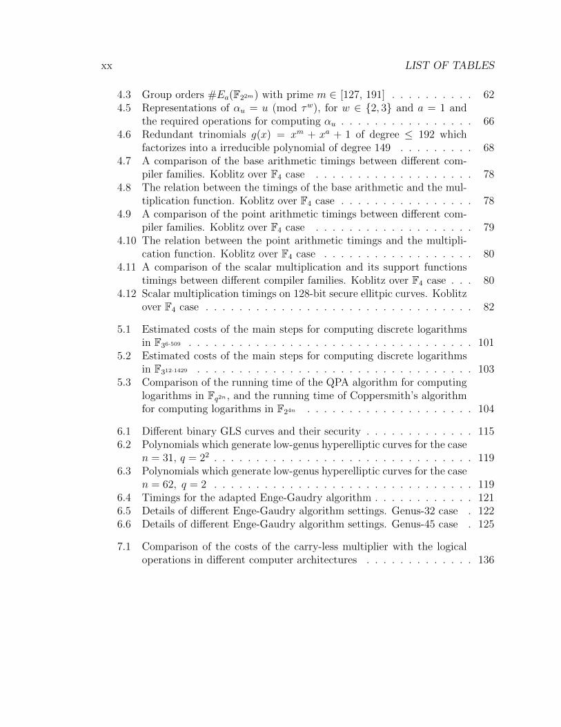
xx LIST OF TABLES
4.3 Group orders #Ea(F22m) with prime m ∈ [127, 191] . . . . . . . . . . 624.5 Representations of αu = u (mod τw), for w ∈ {2, 3} and a = 1 and
the required operations for computing αu . . . . . . . . . . . . . . . . 664.6 Redundant trinomials g(x) = xm + xa + 1 of degree ≤ 192 which
factorizes into a irreducible polynomial of degree 149 . . . . . . . . . 684.7 A comparison of the base arithmetic timings between different com-
piler families. Koblitz over F4 case . . . . . . . . . . . . . . . . . . . 784.8 The relation between the timings of the base arithmetic and the mul-
tiplication function. Koblitz over F4 case . . . . . . . . . . . . . . . . 784.9 A comparison of the point arithmetic timings between different com-
piler families. Koblitz over F4 case . . . . . . . . . . . . . . . . . . . 794.10 The relation between the point arithmetic timings and the multipli-
cation function. Koblitz over F4 case . . . . . . . . . . . . . . . . . . 804.11 A comparison of the scalar multiplication and its support functions
timings between different compiler families. Koblitz over F4 case . . . 804.12 Scalar multiplication timings on 128-bit secure ellitpic curves. Koblitz
over F4 case . . . . . . . . . . . . . . . . . . . . . . . . . . . . . . . . 82
5.1 Estimated costs of the main steps for computing discrete logarithmsin F36·509 . . . . . . . . . . . . . . . . . . . . . . . . . . . . . . . . . . 101
5.2 Estimated costs of the main steps for computing discrete logarithmsin F312·1429 . . . . . . . . . . . . . . . . . . . . . . . . . . . . . . . . . 103
5.3 Comparison of the running time of the QPA algorithm for computinglogarithms in Fq2n , and the running time of Coppersmith’s algorithmfor computing logarithms in F24n . . . . . . . . . . . . . . . . . . . . 104
6.1 Different binary GLS curves and their security . . . . . . . . . . . . . 1156.2 Polynomials which generate low-genus hyperelliptic curves for the case
n = 31, q = 22 . . . . . . . . . . . . . . . . . . . . . . . . . . . . . . . 1196.3 Polynomials which generate low-genus hyperelliptic curves for the case
n = 62, q = 2 . . . . . . . . . . . . . . . . . . . . . . . . . . . . . . . 1196.4 Timings for the adapted Enge-Gaudry algorithm . . . . . . . . . . . . 1216.5 Details of different Enge-Gaudry algorithm settings. Genus-32 case . 1226.6 Details of different Enge-Gaudry algorithm settings. Genus-45 case . 125
7.1 Comparison of the costs of the carry-less multiplier with the logicaloperations in different computer architectures . . . . . . . . . . . . . 136

List of Algorithms
1 Modular reduction by trinomial f(x) = x127 + x63 + 1 . . . . . . . . . 242 Modular reduction by f(x) = x127 + x63 + 1 for the squaring operation 253 GLV-GLS left-to-right double-and-add scalar multiplication . . . . . . 294 GLV-GLS right-to-left halve-and-add scalar multiplication . . . . . . 315 Parallel GLV-GLS scalar multiplication . . . . . . . . . . . . . . . . . 346 Protected GLV-GLS scalar multiplication . . . . . . . . . . . . . . . . 367 Left-to-right Montgomery ladder [114] . . . . . . . . . . . . . . . . . 438 Montgomery-LD double-and-add scalar multiplication (right-to-left) . 459 Montgomery-LD halve-and-add scalar multiplication (right-to-left) . . 4610 Parallel Montgomery-GLV-GLS ladder scalar multiplication (four-core) 4911 Data veiling procedure . . . . . . . . . . . . . . . . . . . . . . . . . . 5112 Regular width-w τ -adic expansion for an m-bit scalar . . . . . . . . . 5813 Timing attack resistant scalar multiplication for Koblitz curves . . . . 5814 Partial reduction on Koblitz curves defined over F4 . . . . . . . . . . 6415 Regular width-w τ -recoding on Koblitz curves defined over F4 . . . . 6516 Modular reduction by the trinomial g(x) = x192 + x19 + 1 . . . . . . . 6717 Mul-and-add reduction modulo the 69-term irreducible polynomial f(x) 6918 Karatsuba algorithm for multiplying three 64-bit word polynomials . 7119 Modular reduction of the terms a0, a1 of an element a = (a0 + a1u)
modulo g(x) = x192 + x19 + 1 . . . . . . . . . . . . . . . . . . . . . . 7220 Squaring of an element a = (a0 + a1u) ∈ F22·149 . . . . . . . . . . . . . 7321 Left-to-right regular w-TNAF τ -and-add on Koblitz curves defined
over F4 . . . . . . . . . . . . . . . . . . . . . . . . . . . . . . . . . . . 7422 Right-to-left regular w-TNAF τ -and-add on Koblitz curves defined
over F4 . . . . . . . . . . . . . . . . . . . . . . . . . . . . . . . . . . . 7523 Linear pass using 128-bit AVX vectorial instructions . . . . . . . . . . 7624 A mechanism for verifying the binary curve parameter b against the
gGHS attack . . . . . . . . . . . . . . . . . . . . . . . . . . . . . . . . 118
xxi

xxii LIST OF ALGORITHMS

1 | Introduction
Extension fields of small characteristic are quite useful for implementing crypto-graphic primitives. This is because their elements can be directly represented in thebinary or ternary number system, which is inherent to the modern computers basedon integrated circuits. As a consequence, the small-characteristic field arithmeticfunctions are usually more efficient when compared with large prime fields.
For instance, let us consider the basic two-word schoolbook multiplication. Wewant to multiply two field elements c = a × b, where each of them is stored intwo machine registers, namely, (a0, a1) and (b0, b1). The schoolbook multiplicationoperation is depicted in Figure 1.1.
Figure 1.1: The two-word schoolbook multiplication
Given that our architecture is embedded with native multipliers with and withoutcarry, which is the case of modern high-end desktops and smart devices, the fourmultiplication operations (a0 × b0), (a1 × b0), (a0 × b1) and (a1 × b1) are similar in
1

2 CHAPTER 1. INTRODUCTION
terms of efficiency for the binary and the prime field cases1,2.However, when we analyze the schoolbook addition phase, the costs differ between
the large and small-characteristic fields. If we consider binary fields constructedwith a polynomial basis, the addition function is realized easily with the exclusive-orlogical operator, since the polynomials that represent the field elements are addedcoefficient-wise and reduced modulo two. As a result, it is not required to man-age carries. On the other hand, in large characteristic fields, we must control thecarry values that could appear during the intermediate additions, with makes theimplementation more cumbersome and, consequently, less efficient.
Considering the advantage, in terms of efficiency, of the small-characteristic fields,one could ask: why aren’t those fields prevalent in real-world cryptographic proto-cols? The reason is that, in terms of security, the structure inherent to cryptographicprimitives constructed over small-characteristic fields allows a wider and more pow-erful range of attacks. If we consider the binary elliptic curves, different approachesfor solving the discrete logarithm problem (ECDLP) were devised in the last decades[58]. In small-characteristic fields, impressive progress in solving the DLP were ob-served in the last five years, which culminated in a quasi-polynomial algorithm [13].
1.1 Motivation
In short, we have currently the following scenario. On the one hand, there existdifferent options for selecting efficient and elegant small-characteristic field primitiveswhich are well-suited for implementation on a wide range of software and hardwarearchitectures. On the other hand, strong and effective approaches for solving themathematical problems beneath those structures were proposed recently and theirprogress seem to continue. These circunstances have brought a considerable levelof suspiciousness in the community on applying cryptographic primitives based onsmall-characteristic fields to the real-world activities.
In this thesis, we intend to clarify the practical implications of the new advanceson the security of small-characteristic field-based primitives and, at the same time,demonstrate that those primitives are highly efficient and should be considered in
1In current high-end desktop platforms (e.g. Intel Haswell) the 64-bit carry-less multiplier has alatency of 7 clock cycles [130], while the 64-bit multiplication with carry is available with a latencyof 4 clock cycles [52].
2For fields of small characteristic greater than two, the multiplication is more costly in software.This is because there are no native instructions which implement the operation in such fields. Onesolution is to implement the multiplication via the expensive comb methods and/or to use a look-uptable approach.
1.2. OUTLINE 3
cryptographic libraries, standards and protocols.
1.2 Outline
This document is divided into two parts. In the first part, denoted high-speed ellipticcurve cryptography, we focus on the constructive aspects of the small-characteristicfield cryptography. More precisely, we present software implementations of the scalarmultiplication algorithm on elliptic curves defined over binary fields.
In Chapter 2, we introduce a novel system of projective coordinates called lambdacoordinates. Its formulas for point addition, doubling and doubling-and-additionare presented with their respective proofs. In addition, we compare the cost forcomputing the point arithmetic operations with state-of-the-art coordinate systems.This work was realized along with Diego F. Aranha, Julio Lopez and FranciscoRodrıguez-Henrıquez and published in [119, 120].
Chapter 3 describes 128-bit scalar multiplication implementations on a Galbraith-Lin-Scott (GLS) curve defined over the quadratic field F22·127 . After giving the detailsof our base and quadratic field arithmetic, we present a protected and non-protectedversion of the point multiplication algorithm designed with the Gallant-Lambert-Vanstone method. Finally, we propose and implement new procedures in order tocompute the Montgomery ladder with the halve-and-add and double-and-add ap-proaches. The work presented in this chapter is based on the papers [119, 120, 118],coauthored with Diego F. Aranha, Julio Lopez and Francisco Rodrıguez-Henrıquez.
In Chapter 4, we devise methods for implementing timing-resistant point multi-plication algorithms on Koblitz curves. At first, we give details of an adaptation ofthe regular recoding procedure proposed by Joye-Tunstall [91] to scalars representedin the τ -adic form. Next, we propose a new family of Koblitz curves defined overF4, which resulted in the fastest protected 128-bit secure point multiplication onthose curves. The advances presented in this chapter are a joint work with DiegoF. Aranha, Julio Lopez and Francisco Rodrıguez-Henrıquez and were partially pub-lished in [118].
In the following paragraphs, we present the outline of the second part of thisthesis, entitled discrete logarithm problem. In these chapters, we analyzed and im-plemented algorithms that solve the discrete logarithm problem (DLP) on small-characteristic fields of cryptographic interest and on binary GLS curves.
Chapter 5 describes the recent advances on solving the DLP on small-characteristicfields and presents implementations of those attacks against two pairing-friendlyfields, specifically, F36·137 and F36·163 . In addition, we analyze concretely the impact
4 CHAPTER 1. INTRODUCTION
of the new approaches in other fields of cryptographic interest, namely, F36·509 andF36·1429 . This work is related to different papers [2, 1, 4, 3], which were couthoredwith Gora Adj, Alfred Menezes and Francisco Rodrıguez-Henrıquez.
In Chapter 6, we present an implementation of the Gaudry-Hess-Smart attack(GHS) against a binary GLS curve defined over the field F22·31 . Also, we presentthe practical implications of constructing a dynamic factor base, as proposed in [85],in the relations collection phase of the Enge-Gaudry algorithm for solving the DLPon hyperelliptic curves. This work was published in [36] and was performed withJesus-Javier Chi.
Finally, in Chapter 7, we conclude the thesis by listing more specifically our maincontributions, a collection of open problems and further research themes related toour main subjects of study.

Part I
High-Speed Elliptic CurveCryptography

2 | Lambda Coordinates
From the algorithmic point of view, one of the most effective approaches to accel-erate the computation of the scalar multiplication is the improvement of the pointarithmetic formulas. The quest for simpler formulas, along with the relatively highcost of the field inversion operation, which is required by the arithmetic of pointsrepresented in affine coordinates, motivated the development of distinct projectivecoordinate systems.
In the case of binary curves, one of the first proposals1 was the homogeneousprojective coordinates system [114, 5], which represents an affine point P = (x, y)as the triplet (X, Y, Z), where x = X
Zand y = Y
Z; whereas in the Jacobian coordi-
nate system [37], a projective point P = (X, Y, Z) corresponds to the affine point(x = X
Z2 , y = YZ3 ). In 1998, Lopez-Dahab (LD) coordinates [105] were introduced,
representing the affine-coordinate x = XZ
and y = YZ2 .
Since then, LD coordinates have become the most studied coordinate system forbinary elliptic curves, with many authors [94, 101, 8, 100, 21] contributing to improvetheir performance. In 2007, Kim and Kim [93] presented a 4-dimensional extensionof the LD coordinate system that represents P as (X, Y, Z, T 2), with x = X
Z, y = Y
T
and T = Z2. In a different vein, Bernstein et al. introduced in [21] a set of completeformulas2 for binary Edwards elliptic curves.
Alternatively, we have different affine representations for binary elliptic points,namely, (x, y
x) and (x, x+ y
x), which were introduced in [95, 139]. In [139] the latter
representation was designated λ-affine representation of points, and was used forperforming the point doubling operation in [105, 106, 139], the point halving in[95, 140, 53, 11], and point compression in [107].
The efficiency of a coordinate system is measured by counting the number of field
1The homogeneous projective coordinates were originally proposed to accelerate integer factor-ization methods based on the elliptic curves [114].
2Given a field K, a complete system of addition laws on an elliptic curve E/K has the propertythat for any two points P,Q ∈ E(K), there is an addition law in the collection that can be used toadd P and Q [32].
7
8 CHAPTER 2. LAMBDA COORDINATES
operations required to perform the point arithmetic functions, namely, addition anddoubling. Usually, only the field multiplication, squaring and inversion operationsare considered, since the costs of the other functions, such as the addition, are usuallynegligible3
Also, when presenting coordinate systems costs and formulas, we frequently sep-arate the point addition into two kinds: full or projective, and mixed. Given twopoints P = (XP , YP , ZP ) and Q = (XQ, YQ, ZQ), both in projective coordinates, thepoint full addition is the operation
R = (XR, YR, ZR) = P +Q.
The mixed point addition is quite similar: given a point P = (XP , YP , ZP ) in projec-tive coordinates and a point Q = (xQ, yQ) in affine coordinates, the mixed additionis the operation R = (XR, YR, ZR) = P + Q. The motives for dividing the pointaddition into different categories, are twofold: first, the mixed addition is less expen-sive than the full addition. In the former, one has that, the coordinate ZQ is equalto one. Consequently, a few field multiplications are saved. Second, different scalarmultiplication algorithms require the computation of a distinct amount of mixed andfull point multiplication functions. As a result, point multiplication estimations canbe made more reliable and concrete if we consider the aforementioned operationsseparately.
2.1 Coordinate systems
In this section, we describe the main binary projective coordinate system formulas forcomputing the point doubling and full addition. The mixed addition can be derivedfrom the full addition formula by taking the normalized version of the projective co-ordinate. Following the scope of this thesis, we only describe the coordinate systemsrelated to Weierstrass binary elliptic curves:
E/F2m : y2 + xy = x3 + ax2 + b. (2.1)
3This statement is only true for the binary field arithmetic implemented in high-end desktops. Inthe near future, it is expected that the difference between the binary field addition and multiplicationcosts become smaller (see Section 7.3.1).

2.1. COORDINATE SYSTEMS 9
2.1.1 Affine coordinates
Theorem 1 ([152, Section 2.8]). Let P = (xP , yP ) be a point in a non-supersingularelliptic curve. Then the formula for computing R = 2P = (xR, yR) is given by:
λ = xP + yP/xP
xR = λ2 + λ+ a
yR = λ · (xP + xR) + xR + yP .
Therefore, one inversion, two multiplications and one squaring are required toperform point doubling in affine coordinates.
Theorem 2 ([152, Section 2.8]). Let P = (xP , yP ) and Q = (xQ, yQ) be points ina non-supersingular elliptic curve, with P 6= ±Q. Then the formula for computingR = P +Q = (xR, yR) is given by:
λ = (yP + yQ)/(xP + xQ)
xR = λ2 + λ+ xP + xQ + a
yR = λ · (xP + xR) + xR + yP .
Then, we need one inversion, two multiplications and one squaring to performthe point addition in affine coordinates.
2.1.2 Homogeneous projective coordinates
Theorem 3 ([114]). Let P = (XP , YP , ZP ) be a point in a non-supersingular ellipticcurve. Then the formula for computing R = 2P = (XR, YR, ZR) is given by:
A = XP · ZPB = b · Z4
P +X4P
XR = A ·BYR = X4
P · A+B · (X2P + YP · ZP + A)
ZR = A3.
As a result, seven multiplications and five squarings are needed to implement thepoint doubling in homogeneous coordinates.
Theorem 4 ([114]). Let P = (XP , YP , ZP ) and Q = (XQ, YQ, ZQ) be points in anon-supersingular elliptic curve, with P 6= ±Q. Then the formula for computing

10 CHAPTER 2. LAMBDA COORDINATES
R = P +Q = (XR, YR, ZR) is given by:
A = XQ · ZP +XP · ZQB = YQ · ZP + YP · ZQC = A+B
D = A2 · (A+ a · ZP · ZQ) + ZP · ZQ ·B · CXR = A ·DYR = C ·D + A2 · (B ·XP + A · YP )
ZR = A3 · ZP · ZQ.
Here, we need sixteen multiplications and one squaring to implement the point fulladdition in homogeneous coordinates.
2.1.3 Jacobian projective coordinates
The Jacobian coordinates formulas described in this section are based on [19].
Theorem 5 ([37]). Let P = (XP , YP , ZP ) be a point in a non-supersingular ellipticcurve. Then the formula for computing R = 2P = (XR, YR, ZR) is given by:
A = X2P
B = A2
C = Z2P
D = C2
XR = B + b ·D2
ZR = XP · CYR = B · ZR + (A+ YP · ZP + ZR) ·XR.
As a consequence, five multiplications and five squarings are required to implementthe point doubling in Jacobian coordinates.
Theorem 6 ([37]). Let P = (XP , YP , ZP ) and Q = (XQ, YQ, ZQ) be points in anon-supersingular elliptic curve, with P 6= ±Q. Then the formula for computing
2.1. COORDINATE SYSTEMS 11
R = P +Q = (XR, YR, ZR) is given by:
A = XP · Z2Q +XQ · Z2
P
B = YP · Z3Q + YQ · Z3
P
C = A · ZPD = B ·XQ + C · YQZR = C · ZQE = B + ZR
XR = a · Z2R +B · E + A3
YR = E ·XR + C2 ·D.
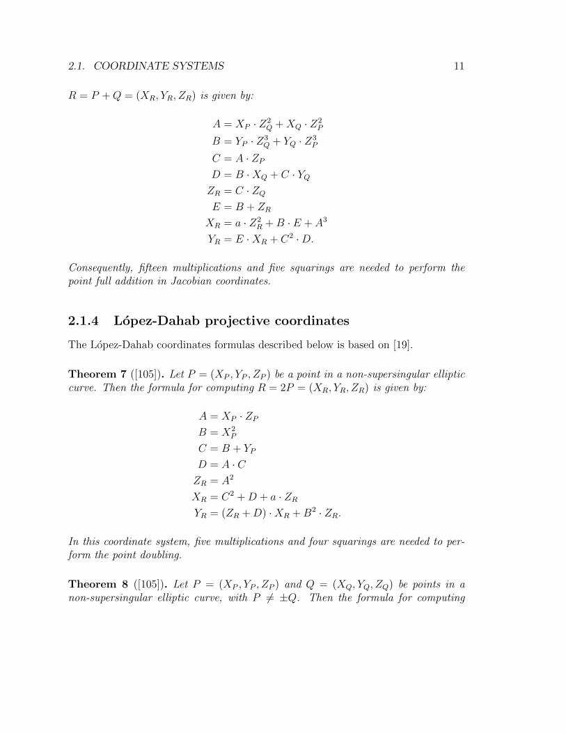
Consequently, fifteen multiplications and five squarings are needed to perform thepoint full addition in Jacobian coordinates.
2.1.4 Lopez-Dahab projective coordinates
The Lopez-Dahab coordinates formulas described below is based on [19].
Theorem 7 ([105]). Let P = (XP , YP , ZP ) be a point in a non-supersingular ellipticcurve. Then the formula for computing R = 2P = (XR, YR, ZR) is given by:
A = XP · ZPB = X2
P
C = B + YP
D = A · CZR = A2
XR = C2 +D + a · ZRYR = (ZR +D) ·XR +B2 · ZR.
In this coordinate system, five multiplications and four squarings are needed to per-form the point doubling.
Theorem 8 ([105]). Let P = (XP , YP , ZP ) and Q = (XQ, YQ, ZQ) be points in anon-supersingular elliptic curve, with P 6= ±Q. Then the formula for computing
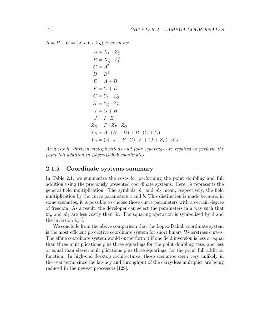
12 CHAPTER 2. LAMBDA COORDINATES
R = P +Q = (XR, YR, ZR) is given by:
A = XP · Z2Q
B = XQ · Z2P
C = A2
D = B2
E = A+B
F = C +D
G = YP · Z2Q
H = YQ · Z2P
I = G+H
J = I · EZR = F · ZP · ZQXR = A · (H +D) +B · (C +G)
YR = (A · J + F ·G) · F + (J + ZR) ·XR.
As a result, thirteen multiplications and four squarings are required to perform thepoint full addition in Lopez-Dahab coordinates.
2.1.5 Coordinate systems summary
In Table 2.1, we summarize the costs for performing the point doubling and fulladdition using the previously presented coordinate systems. Here, m represents thegeneral field multiplication. The symbols ma and mb mean, respectively, the fieldmultiplication by the curve parameters a and b. This distinction is made because, insome scenarios, it is possible to choose those curve parameters with a certain degreeof freedom. As a result, the developer can select the parameters in a way such thatma and mb are less costly than m. The squaring operation is symbolized by s andthe inversion by i.
We conclude from the above comparison that the Lopez-Dahab coordinate systemis the most efficient projective coordinate system for short binary Weierstrass curves.The affine coordinate system would outperform it if one field inversion is less or equalthan three multiplications plus three squarings for the point doubling case, and lessor equal than eleven multiplications plus three squarings, for the point full additionfunction. In high-end desktop architectures, those scenarios seem very unlikely inthe year term, since the latency and throughput of the carry-less multiplier are beingreduced in the newest processors [129].
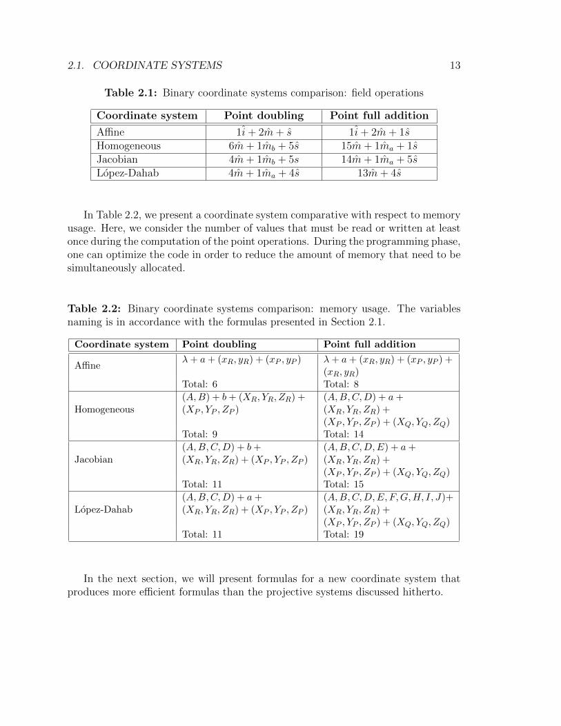
2.1. COORDINATE SYSTEMS 13
Table 2.1: Binary coordinate systems comparison: field operations
Coordinate system Point doubling Point full addition
Affine 1i+ 2m+ s 1i+ 2m+ 1sHomogeneous 6m+ 1mb + 5s 15m+ 1ma + 1sJacobian 4m+ 1mb + 5s 14m+ 1ma + 5sLopez-Dahab 4m+ 1ma + 4s 13m+ 4s
In Table 2.2, we present a coordinate system comparative with respect to memoryusage. Here, we consider the number of values that must be read or written at leastonce during the computation of the point operations. During the programming phase,one can optimize the code in order to reduce the amount of memory that need to besimultaneously allocated.
Table 2.2: Binary coordinate systems comparison: memory usage. The variablesnaming is in accordance with the formulas presented in Section 2.1.
Coordinate system Point doubling Point full addition
Affineλ+ a+ (xR, yR) + (xP , yP ) λ+ a+ (xR, yR) + (xP , yP ) +
(xR, yR)Total: 6 Total: 8
Homogeneous(A,B) + b+ (XR, YR, ZR) +(XP , YP , ZP )
(A,B,C,D) + a+(XR, YR, ZR) +(XP , YP , ZP ) + (XQ, YQ, ZQ)
Total: 9 Total: 14
Jacobian(A,B,C,D) + b+(XR, YR, ZR) + (XP , YP , ZP )
(A,B,C,D,E) + a+(XR, YR, ZR) +(XP , YP , ZP ) + (XQ, YQ, ZQ)
Total: 11 Total: 15
Lopez-Dahab(A,B,C,D) + a+(XR, YR, ZR) + (XP , YP , ZP )
(A,B,C,D,E, F,G,H, I, J)+(XR, YR, ZR) +(XP , YP , ZP ) + (XQ, YQ, ZQ)
Total: 11 Total: 19
In the next section, we will present formulas for a new coordinate system thatproduces more efficient formulas than the projective systems discussed hitherto.

14 CHAPTER 2. LAMBDA COORDINATES
2.2 Lambda projective coordinates
As seen in the previous section, in order to have a more efficient elliptic curve arith-metic, it is standard to use a projective version of the Weierstrass elliptic curveequation (2.1), where the points are represented in the so-called projective space. Inthe following, we describe the λ-projective coordinates, a coordinate system whoseassociated group law is introduced in this part.
Given a point P = (xP , yP ) ∈ E(F2m) with xP 6= 0, the λ-affine representa-tion of P is defined as (xP , λP ), where λP = xP + yP
xP. The λ-projective point
P = (XP , LP , ZP ) corresponds to the λ-affine point (XPZP, LPZP
). The λ-projective equa-tion form of the Weierstrass equation (2.1) is,
(L2 + LZ + aZ2)X2 = X4 + bZ4. (2.2)
Notice that the condition xP = 0 does not pose a limitation in practice, since theonly point P with xP = 0 that satisfies equation (2.1) is (0,
√b), which is usually
confined to a subgroup of no cryptographic interest.
2.2.1 Group law
In this section, the formulas for point doubling and addition in the λ-projectivecoordinate system are presented. Complementary formulas, when they exist, andcomplete proofs follow each given formula.
Theorem 9. Let P = (XP , LP , ZP ) be a point in a non-supersingular curve. Thenthe formula for computing R = 2P = (XR, LR, ZR) using the λ-projective represen-tation is given by
A = L2P + (LP · ZP ) + a · Z2
P
XR = A2
ZR = A · Z2P
LR = (XP · ZP )2 +XR + A · (LP · ZP ) + ZR.
As a result, five multiplications and four squarings are required to perform thepoint doubling in λ-projective coordinates.
For situations where the multiplication by the b-coefficient is fast, one can replacea standard multiplication with a multiplication by the constant (a2 + b). We presentbelow an alternative formula for calculating LR:
LR = (LP +XP )2 · ((LP +XP )2 + A+ Z2P ) + (a2 + b) · Z4
P +XR + (a+ 1) · ZR.
2.2. LAMBDA PROJECTIVE COORDINATES 15
Proof of Theorem 9. Let P = (xP , λP ) be a point in an non-supersingular curve.Then a formula for computing R = 2P = (xR, λR) is given by
xR = λ2P + λP + a
λR =x2P
xR+ λ2
P + a+ 1.
From [78, Section 3.1.2], we have the formulas: xR = λ2P + λP + a and yR = x2
P +λPxR + xR. Then, a formula for computing λR can be obtained as follows:
λR =yR + x2
R
xR=
(x2P + λP · xR + xR) + x2
R
xR
=x2P
xR+ λP + 1 + xR =
x2P
xR+ λP + 1 + (λ2
P + λP + a)
=x2P
xR+ λ2
P + a+ 1.
In affine coordinates, the doubling formula requires one division and two squarings.Given the point P = (XP , LP , ZP ) in the λ-projective representation, an efficientprojective doubling algorithm can be derived by applying the doubling formula tothe affine point (XP
ZP, LPZP
). For xR we have:
xR =L2P
Z2P
+LPZP
+ a =L2P + LP · ZP + a · Z2
P
Z2P
=A
Z2P
=A2
A · Z2P
.
For λR we have:
λR =
X2P
Z2P
TZ2P
+L2P
Z2P
+ a+ 1
=X2P · Z2
P + A · (L2P + (a+ 1) · Z2
P )
A · Z2P
.
From the λ-projective equation, we have the relation A · X2P = X4
P + b · Z4P . Then
16 CHAPTER 2. LAMBDA COORDINATES
the numerator w of λR can also be written as follows,
w = X2P · Z2
P + A · (L2P + (a+ 1) · Z2
P )
= X2P · Z2
P + A · L2P + A2 + A2 + (a+ 1) · ZR
= X2P · Z2
P + A · L2P + L4
P + L2P · Z2
P + a2 · Z4P + A2 + (a+ 1) · ZR
= X2P · Z2
P + A · (L2P +X2
P ) +X4P + b · Z4
P + L4P
+ L2P · Z2
P + a2 · Z4P + A2 + (a+ 1) · ZR
= (L2P +X2
P ) · ((L2P +X2
P ) + A+ Z2P ) + A2
+ (a2 + b) · Z4P + (a+ 1) · ZR.
This completes the proof.
Theorem 10. Let P = (XP , LP , ZP ) and Q = (XQ, LQ, ZQ) be points in a non-supersingular curve, with P 6= ±Q. Then the addition R = P + Q = (XR, LR, ZR)can be computed by the formulas
A = LP · ZQ + LQ · ZPB = (XP · ZQ +XQ · ZP )2
XR = A · (XP · ZQ) · (XQ · ZP ) · ALR = (A · (XQ · ZP ) +B)2 + (A ·B · ZQ) · (LP + ZP )
ZR = (A ·B · ZQ) · ZP .
Proof of Theorem 10. Let P = (xP , λP ) and Q = (xQ, λQ) be elliptic curve points.Then a formula for R = P +Q = (xR, λR) is given by
xR =xP · xQ
(xP + xQ)2(λP + λQ)
λR =xQ · (xR + xP )2
xR · xP+ λP + 1.
Since P and Q are elliptic points on a non-supersingular curve, we have the followingrelation: y2
P + xP · yP + x3P + a · x2
P = b = y2Q + xQ · yQ + x3
Q + a · x2Q. The known
formula for computing the x-coordinate of R is given by xR = s2 + s+ xP + xQ + a,
2.2. LAMBDA PROJECTIVE COORDINATES 17
where s =yP+yQxP+xQ
. Then one can derive the new formula as follows,
xR =(yP + yQ)2 + (yP + yQ) · (xP + yQ)
(xP + xQ)2
+(xP + xQ)3 + a · (xP + xQ)2
(xP + xQ)2
=b+ b+ xQ · (x2
P + yP ) + xP · (x2Q + yQ)
(xP + xQ)2
=xP · xQ · (λP + λQ)
(xP + xQ)2.
For computing λR, we use the observation that the x-coordinate of R − P is xQ.We also know that for −P we have λ−P = λP + 1 and x−P = xP . By applying theformula for the x-coordinate of R + (−P ) we have
xQ = xR+(−P ) =xR · x−P
(xR + x−P )2· (λR + λ−P )
=xR · xP
(xR + xP )2· (λR + λP + 1).
Then λR =xQ·(xR+xP )2
xR·xP+ λP + 1.
To obtain a λ-projective addition formula, we apply the formulas above to theaffine points (XP
ZP, LPZP
) and (XQZQ,LQZQ
). Then, the xR coordinate of P + Q can be
computed as:
xR =
XPZP· XQZQ· (LP
ZP+
LQZQ
)
(XPZP
+XQZQ
)2
=XP ·XQ · (LP · ZQ + LQ · ZP )
(XP · ZQ +XQ · ZP )2= XP ·XQ ·
A
B.
For the λR coordinate we have:
λR =
XQZQ· (XP ·XQ·A
B+ XP
ZP)2
XP ·XQ·AB
· XPZP
+LP + ZPZP
=(A ·XQ · ZP +B)2 + (A ·B · ZQ)(LP + ZP )
A ·B · ZP · ZQ.
18 CHAPTER 2. LAMBDA COORDINATES
In order that both xR and λR have the same denominator, the formula for xR canbe written as
XR =XP ·XQ · A
B=A · (XP · ZQ) · (XQ · ZP ) · A
A ·B · ZP · ZQ.
Therefore, xR = XRZR
and λR = LRZR
. This completes the proof.
Furthermore, we derived an efficient formula for computing the operation R =2Q+P , with the points Q and P represented in λ-projective and λ-affine coordinates,respectively.
Theorem 11. Let P = (xP , λP ) and Q = (XQ, LQ, ZQ) be points in a non-supersingular curve. Then the operation R = 2Q+P = (XR, LR, ZR) can be computedas follows:
A = L2Q + LQ · ZQ + a · Z2
Q
B = X2Q · Z2
Q + A · (L2Q + (a+ 1 + λP ) · Z2
Q)
C = (xP · Z2Q + A)2
XR = (xP · Z2Q) ·B2
ZR = (B · C · Z2Q)
LR = A · (B + C)2 + (λP + 1) · ZR.Proof of Theorem 11. The λ-projective formula is obtained by adding the λ-affinepoints S = 2Q = (xS, λS) = (XS
ZS, LSZS
) and P = (xP , λP ) with the formula of Theorem2. Then, the x coordinate of R = S + P is given by
xR =xS · xP
(xS + xP )2(λS + λP )
=XS · xP (LS + λP · ZS)
(XS + xP · ZS)2
=xP · (X2
Q · Z2Q + A · (L2
Q + (a+ 1 + λP ) · Z2Q))
(T + xP · Z2Q)2
= xP ·B
C.
The λR coordinate of S + P is computed as
λR =
XSZS· (xP · BC + xP )2
xP · BC · xP+ λP + 1
=A · (B + C)2 + (λP + 1) · (B · C · Z2
Q)
B · C · Z2Q
.
2.2. LAMBDA PROJECTIVE COORDINATES 19
The formula for xR can be written with denominator ZR as follows,
xR =xP ·BC
=xP · Z2
Q ·B2
B · C · Z2Q
.
Therefore, xR = XRZR
and λR = LRZR
. This completes the proof.
2.2.2 Comparison
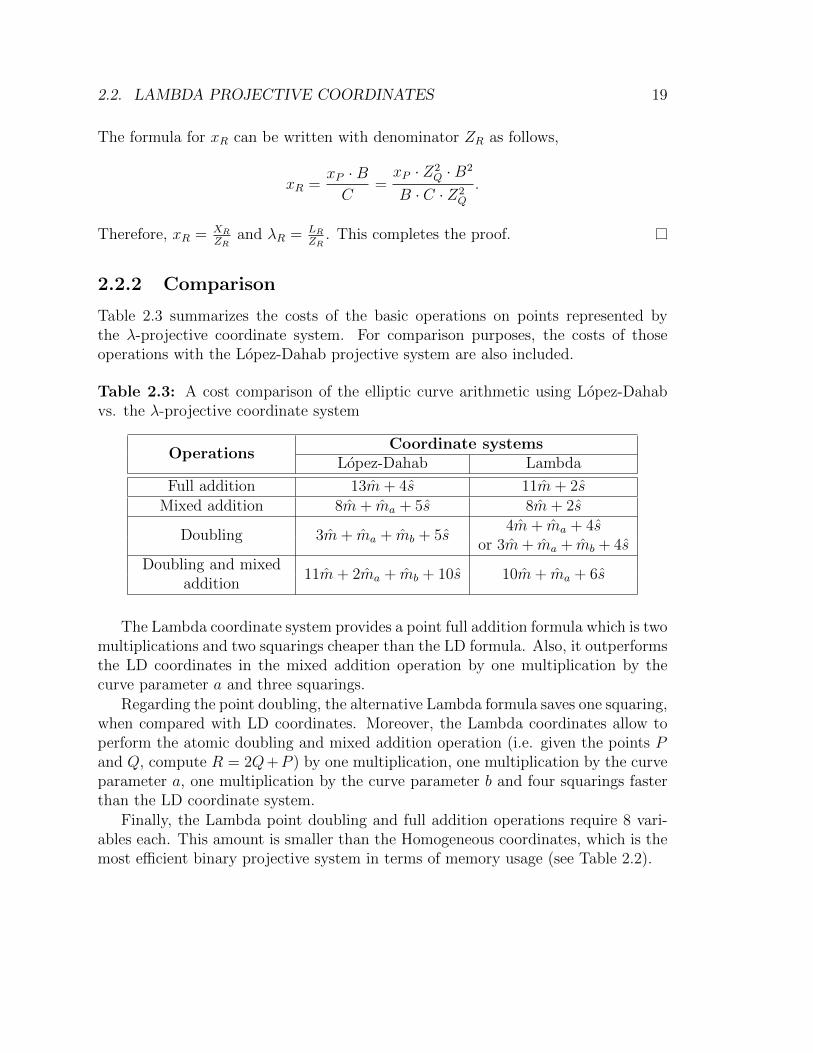
Table 2.3 summarizes the costs of the basic operations on points represented bythe λ-projective coordinate system. For comparison purposes, the costs of thoseoperations with the Lopez-Dahab projective system are also included.
Table 2.3: A cost comparison of the elliptic curve arithmetic using Lopez-Dahabvs. the λ-projective coordinate system
OperationsCoordinate systems
Lopez-Dahab Lambda
Full addition 13m+ 4s 11m+ 2sMixed addition 8m+ ma + 5s 8m+ 2s
Doubling 3m+ ma + mb + 5s4m+ ma + 4s
or 3m+ ma + mb + 4sDoubling and mixed
11m+ 2ma + mb + 10s 10m+ ma + 6saddition
The Lambda coordinate system provides a point full addition formula which is twomultiplications and two squarings cheaper than the LD formula. Also, it outperformsthe LD coordinates in the mixed addition operation by one multiplication by thecurve parameter a and three squarings.
Regarding the point doubling, the alternative Lambda formula saves one squaring,when compared with LD coordinates. Moreover, the Lambda coordinates allow toperform the atomic doubling and mixed addition operation (i.e. given the points Pand Q, compute R = 2Q+P ) by one multiplication, one multiplication by the curveparameter a, one multiplication by the curve parameter b and four squarings fasterthan the LD coordinate system.
Finally, the Lambda point doubling and full addition operations require 8 vari-ables each. This amount is smaller than the Homogeneous coordinates, which is themost efficient binary projective system in terms of memory usage (see Table 2.2).
20 CHAPTER 2. LAMBDA COORDINATES
2.3 Summary
In this chapter, we presented a survey on the projective coordinate systems forbinary elliptic curves. For each representation, we gave formulas for computing thepoint doubling and full addition operations along with their costs in terms of fieldarithmetic functions.
After that, we introduced a new set of projective coordinates denominated lambdacoordinates. Here, we presented formulas and their respecive proofs for the point dou-bling, mixed addition, full addition and doubling-and-mixed-addition operations.Those operations, computed in lambda coordinates, outperforms, in terms of effi-ciency, the state-of-the-art Lopez-Dahab projective coordinates for binary curves.
3 | Galbraith-Lin-Scott Curves
Given a point P ∈ E(F2m) of prime order r, the average cost of computing the scalarmultiplication Q = kP by a random n-bit scalar k using the traditional double-and-add method is about nD+ n
2A, where D and A are the cost of doubling and adding
a point, respectively.
In 2001, Gallant, Lambert and Vanstone (GLV) [63] presented a technique thatuses efficiently computable endomorphisms, available in certain classes of ellipticcurves, which allows significant speedups in the scalar multiplication computation. Ifthe elliptic curve is equipped with a non-trivial efficiently computable endomorphismψ such that ψ(P ) = δP ∈ 〈P 〉, for some δ ∈ [2, r− 2]. Then the point multiplicationcan be computed through the GLV method as,
Q = kP = k1P + k2ψ(P ) = k1P + k2 · δP,
where the subscalars |k1|, |k2| ≈ n/2, can be found by solving a closest vector prob-lem in a lattice [61]. Having split the scalar k into two parts, the computation ofkP = k1P +k2ψ(P ) can be performed by applying simultaneous multiple point mul-tiplication techniques [78, Section 3.3.3] that translates into a saving of half of thedoublings required by the execution of a single point multiplication kP .
In 2009, Galbraith, Lin and Scott (GLS) [61] constructed efficient endomorphismsfor a broader class of elliptic curves defined over Fp2 , where p is a prime number,showing that the GLV technique also applies to these curves. Subsequently, Hanker-son, Karabina and Menezes investigated in [76] the feasibility of implementing theGLS curves over F22m .
In this chapter, we present efficient implementations of the 128-bit secure scalarmultiplication over binary GLS curves on high-end desktop architectures. Our workprovides an efficient quadratic finite field arithmetic and takes advantage of the GLScurve endomorphism to generate fast timing-attack resistant and non-resistant pointmultiplication algorithms.
21
22 CHAPTER 3. GALBRAITH-LIN-SCOTT CURVES
3.1 Binary field arithmetic
A binary extension field F2m of order q = 2m can be constructed by taking anm-degree polynomial f(x) ∈ F2[x] irreducible over F2. The field F2m is isomor-phic to F2[x]/(f(x)) and its elements are binary polynomials of degree less than m.Quadratic extensions of a binary extension field can be built using a degree two monicpolynomial g(u) ∈ F2[u] that happens to be irreducible over Fq. In this case, thefield Fq2 is isomorphic to Fq[u]/(g(u)) and its elements can be represented as a+ bu,with a, b ∈ Fq. In this chapter, we developed an efficient field arithmetic library forthe field Fq and its quadratic extension Fq2 , with m = 127, which were constructedby means of the irreducible trinomials f(x) = x127 + x63 + 1 and g(u) = u2 + u+ 1,respectively.
The following discussion assumes m = 127, but all techniques can be easilyadapted to other field extensions.
3.1.1 Field multiplication over FqGiven two field elements a, b ∈ Fq, the field multiplication can be performed by poly-nomial multiplication followed by modular reduction as, c = a · b mod f(x). Sincethe binary coefficients of the base field elements Fq can be packed as vectors of two64-bit words, the standard Karatsuba method allows us to compute the polynomialmultiplication step at a cost of three 64-bit products (equivalent to three invoca-tions of the carry-less multiplication instruction [148]), plus some additions. Due tothe very special form of f(x), modular reduction is especially elegant as it can beaccomplished using essentially additions and shifts.
3.1.2 Field squaring, square root and multi-squaring over FqDue to the action of the Frobenius operator, field squaring and square-root are linearoperations in any binary field [136]. These two operations can be implemented ata very low cost provided that the base field Fq is defined by a square-root friendlytrinomial or pentanomial1. Furthermore, vectorized implementations with simulta-neous table look-ups through byte shuffling instructions, as presented in [10], keptsquare and square-root efficient relative to multiplication even with the accelerationof field multiplication brought by the native carry-less multiplier.
1The continuing decrease of the carry-less multiplier costs will probably make this requirementobsolete.
3.1. BINARY FIELD ARITHMETIC 23
Multi-squaring, or exponentiation to 2k, with k > 5 is performed via look-up ofper-field constant tables of field elements, as proposed in [7, 30]. For a fixed k, atable T of 24 · dm
4e field elements can be precomputed such that
T [j, i0 + 2i1 + 4i2 + 8i3] = (i0z4j + i1z
4j+1 + i2z4j+2 + i3z
4j+3)2k
and a2k =∑dm
4e
j=0 T [j, ba/24jc mod 24].
3.1.3 Field inversion over FqField inversion in the base field is carried out using the Itoh-Tsujii algorithm [84],by computing a−1 = a(2m−1−1)2. The exponentiation is computed through the terms(a2i−1)2k · a2k−1, with 0 ≤ i ≤ k ≤ m − 1. The overall cost of the method is m − 1squarings and 9 multiplications given by the length of the following addition chainfor m− 1 = 126,
1→ 2→ 3→ 6→ 12→ 24→ 48→ 96→ 120→ 126.
The cost of squarings can be reduced by computing each required 2k-power as amulti-squaring whenever k > 5. This value was determined experimentally.
3.1.4 Modular reduction
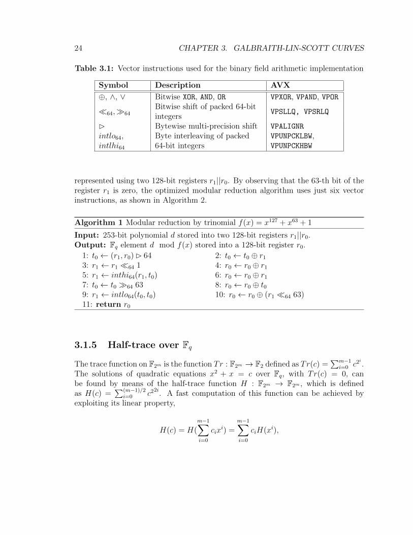
Table 3.1 provides the notation of the vector instructions that were used for perform-ing the modular reduction algorithms to be presented in this section. This notationis closely based on [10], but notice that here, we are invoking the three-operand AVXinstructions corresponding to 128-bit SSE instructions. Bitwise logical instructionsoperate across two entire vector registers and produce the result in a third vectorregister. Bitwise shifts perform parallel shifts in the 64-bit integers packed in avector register, not propagating bits between contiguous data objects and requiringadditional instructions to implement 128-bit shifts. Bytewise shifts are different inboth the shift amount, which must be a multiple of 8; and the propagation of shiftedout bytes between the two operands. Byte interleaving instructions take bytes alter-nately from the lower or higher halves of two vector register operands to produce athird output register.
For our irreducible trinomial f(x) = x127 + x63 + 1 choice, we use the procedureshown in Algorithm 1, which requires ten vector instructions to perform a reduc-tion in the base field Fq. This modular reduction algorithm can be improved whenperforming field squaring. In this case, the 253-bit polynomial a2, with a ∈ Fq, is
24 CHAPTER 3. GALBRAITH-LIN-SCOTT CURVES
Table 3.1: Vector instructions used for the binary field arithmetic implementation
Symbol Description AVX
⊕, ∧, ∨ Bitwise XOR, AND, OR VPXOR, VPAND, VPOR
�64,�64Bitwise shift of packed 64-bit
VPSLLQ, VPSRLQintegers
B Bytewise multi-precision shift VPALIGNR
intlo64,intlhi64
Byte interleaving of packed64-bit integers
VPUNPCKLBW,VPUNPCKHBW
represented using two 128-bit registers r1||r0. By observing that the 63-th bit of theregister r1 is zero, the optimized modular reduction algorithm uses just six vectorinstructions, as shown in Algorithm 2.
Algorithm 1 Modular reduction by trinomial f(x) = x127 + x63 + 1
Input: 253-bit polynomial d stored into two 128-bit registers r1||r0.Output: Fq element d mod f(x) stored into a 128-bit register r0.
1: t0 ← (r1, r0) B 643: r1 ← r1 �64 15: r1 ← inthi64(r1, t0)7: t0 ← t0 �64 639: r1 ← intlo64(t0, t0)11: return r0
2: t0 ← t0 ⊕ r1
4: r0 ← r0 ⊕ r1
6: r0 ← r0 ⊕ r1
8: r0 ← r0 ⊕ t010: r0 ← r0 ⊕ (r1 �64 63)
3.1.5 Half-trace over Fq
The trace function on F2m is the function Tr : F2m → F2 defined as Tr(c) =∑m−1
i=0 c2i .The solutions of quadratic equations x2 + x = c over Fq, with Tr(c) = 0, canbe found by means of the half-trace function H : F2m → F2m , which is definedas H(c) =
∑(m−1)/2i=0 c22i
. A fast computation of this function can be achieved byexploiting its linear property,
H(c) = H(m−1∑i=0
cixi) =
m−1∑i=0
ciH(xi),
3.1. BINARY FIELD ARITHMETIC 25
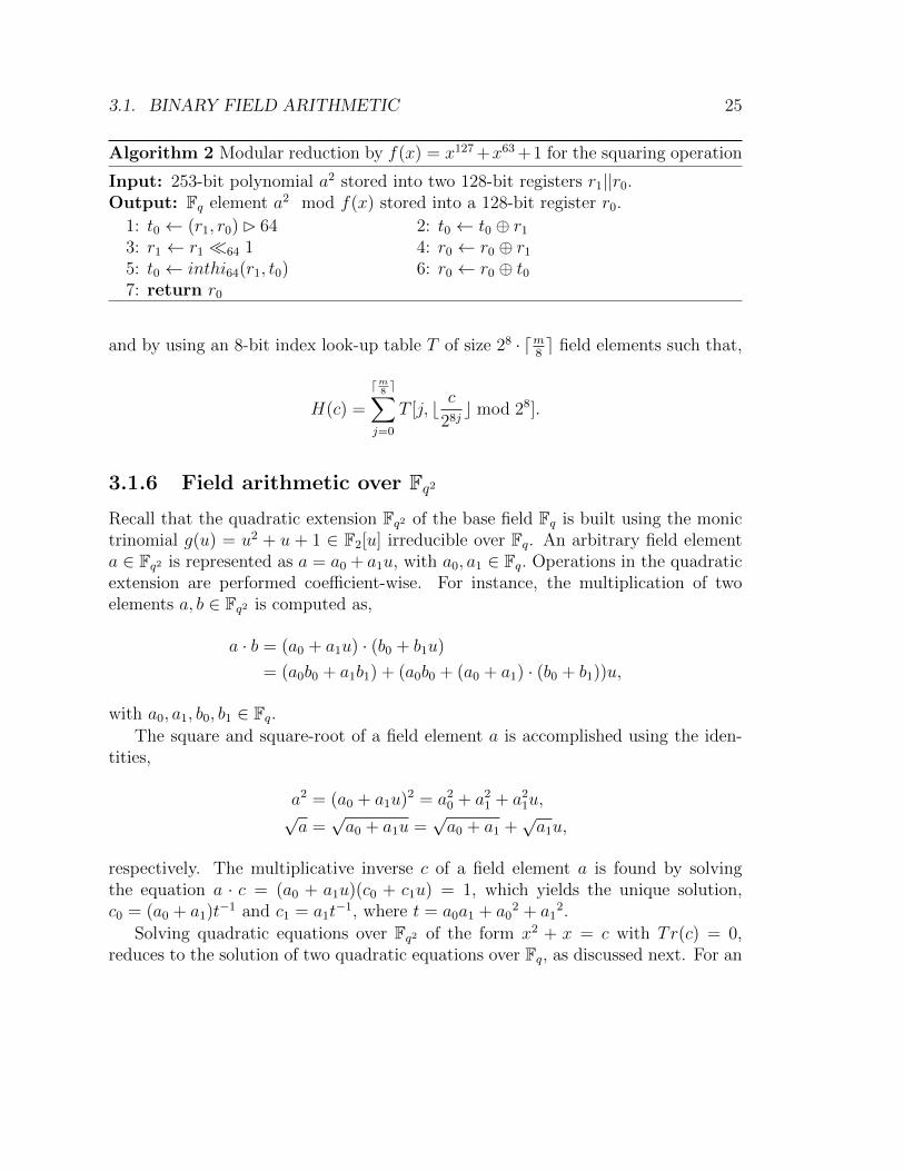
Algorithm 2 Modular reduction by f(x) = x127 +x63 +1 for the squaring operation
Input: 253-bit polynomial a2 stored into two 128-bit registers r1||r0.Output: Fq element a2 mod f(x) stored into a 128-bit register r0.
1: t0 ← (r1, r0) B 643: r1 ← r1 �64 15: t0 ← inthi64(r1, t0)7: return r0
2: t0 ← t0 ⊕ r1
4: r0 ← r0 ⊕ r1
6: r0 ← r0 ⊕ t0
and by using an 8-bit index look-up table T of size 28 · dm8e field elements such that,
H(c) =
dm8e∑
j=0
T [j, b c28jc mod 28].
3.1.6 Field arithmetic over Fq2Recall that the quadratic extension Fq2 of the base field Fq is built using the monictrinomial g(u) = u2 + u + 1 ∈ F2[u] irreducible over Fq. An arbitrary field elementa ∈ Fq2 is represented as a = a0 + a1u, with a0, a1 ∈ Fq. Operations in the quadraticextension are performed coefficient-wise. For instance, the multiplication of twoelements a, b ∈ Fq2 is computed as,
a · b = (a0 + a1u) · (b0 + b1u)
= (a0b0 + a1b1) + (a0b0 + (a0 + a1) · (b0 + b1))u,
with a0, a1, b0, b1 ∈ Fq.The square and square-root of a field element a is accomplished using the iden-
tities,
a2 = (a0 + a1u)2 = a20 + a2
1 + a21u,√
a =√a0 + a1u =
√a0 + a1 +
√a1u,
respectively. The multiplicative inverse c of a field element a is found by solvingthe equation a · c = (a0 + a1u)(c0 + c1u) = 1, which yields the unique solution,c0 = (a0 + a1)t−1 and c1 = a1t
−1, where t = a0a1 + a02 + a1
2.
Solving quadratic equations over Fq2 of the form x2 + x = c with Tr(c) = 0,reduces to the solution of two quadratic equations over Fq, as discussed next. For an
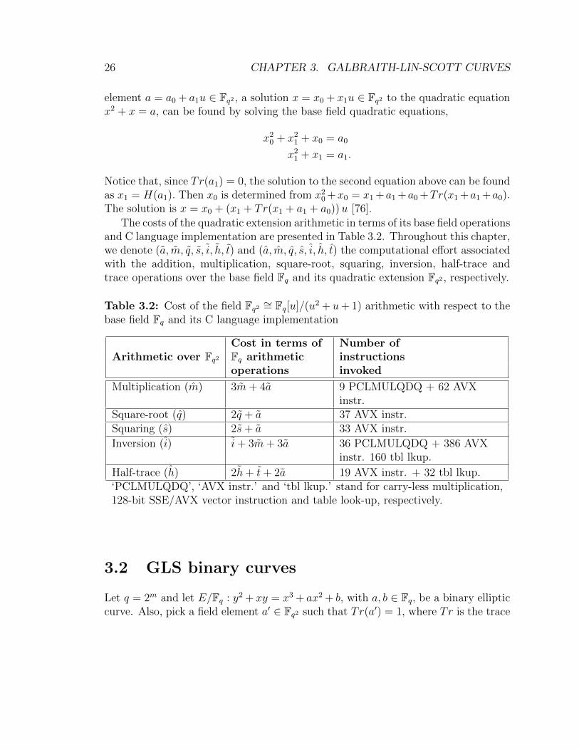
26 CHAPTER 3. GALBRAITH-LIN-SCOTT CURVES
element a = a0 + a1u ∈ Fq2 , a solution x = x0 + x1u ∈ Fq2 to the quadratic equationx2 + x = a, can be found by solving the base field quadratic equations,
x20 + x2
1 + x0 = a0
x21 + x1 = a1.
Notice that, since Tr(a1) = 0, the solution to the second equation above can be foundas x1 = H(a1). Then x0 is determined from x2
0 +x0 = x1 +a1 +a0 +Tr(x1 +a1 +a0).The solution is x = x0 + (x1 + Tr(x1 + a1 + a0))u [76].
The costs of the quadratic extension arithmetic in terms of its base field operationsand C language implementation are presented in Table 3.2. Throughout this chapter,we denote (a, m, q, s, i, h, t) and (a, m, q, s, i, h, t) the computational effort associatedwith the addition, multiplication, square-root, squaring, inversion, half-trace andtrace operations over the base field Fq and its quadratic extension Fq2 , respectively.
Table 3.2: Cost of the field Fq2 ∼= Fq[u]/(u2 + u+ 1) arithmetic with respect to thebase field Fq and its C language implementation
Arithmetic over Fq2Cost in terms of Number ofFq arithmetic instructionsoperations invoked
Multiplication (m) 3m+ 4a 9 PCLMULQDQ + 62 AVXinstr.
Square-root (q) 2q + a 37 AVX instr.Squaring (s) 2s+ a 33 AVX instr.
Inversion (i) i+ 3m+ 3a 36 PCLMULQDQ + 386 AVXinstr. 160 tbl lkup.
Half-trace (h) 2h+ t+ 2a 19 AVX instr. + 32 tbl lkup.‘PCLMULQDQ’, ‘AVX instr.’ and ‘tbl lkup.’ stand for carry-less multiplication,128-bit SSE/AVX vector instruction and table look-up, respectively.
3.2 GLS binary curves
Let q = 2m and let E/Fq : y2 + xy = x3 + ax2 + b, with a, b ∈ Fq, be a binary ellipticcurve. Also, pick a field element a′ ∈ Fq2 such that Tr(a′) = 1, where Tr is the trace

3.2. GLS BINARY CURVES 27
function from Fq2 to F2 (see Section 3.1.5). Given #E(Fq) = q+1− t, it follows that#E(Fq2) = (q + 1)2 − t2. Let us define
E/Fq2 : y2 + xy = x3 + a′x2 + b, (3.1)
with #E(Fq2) = (q − 1)2 + t2. It is known that E is the quadratic twist of E, whichmeans that both curves are isomorphic over Fq4 under the endomorphism [76]
φ : E → E,
(x, y) 7→ (x, y + sx),
with s ∈ Fq4\Fq2 satisfying s2 + s = a+ a′.It is also known that the map φ is an involution, i.e., φ = φ−1. Let π : E → E
be the Frobenius map defined as (x, y) 7→ (x2m , y2m), and let ψ be the compositeendomorphism ψ = φπφ−1 given as,
ψ : E → E,
(x, y) 7→ (x2m , y2m + s2mx2m + sx2m).
In this work, the binary elliptic curve Ea′,b(Fq2) was defined with the parameters
a′ = u and b ∈ Fq, where b was carefully chosen to ensure that #Ea′,b(Fq2) = hr,with h = 2 and where r is a prime of size 2m− 1 bits. Moreover, s2m + s = u, whichimplies that the endomorphism ψ acting over the λ-affine point
P = (x0 + x1u, λ0 + λ1u) ∈ Ea′,b(Fq2),
can be computed with only three additions in Fq as
ψ(P ) 7→ ((x0 + x1) + x1u, (λ0 + λ1) + (λ1 + 1)u).
3.2.1 Security
Given a point Q ∈ 〈P 〉, the elliptic curve discrete logarithm problem (ECDLP)consists of finding the unique integer k ∈ [0, r− 1] such that Q = kP. To the best ofour knowledge, the most powerful attack for solving the ECDLP on binary ellipticcurves was presented in [125] (see also [82, 143]), with an associated computational
complexity of O(2c·m2/3 logm), where c < 2, and where m is a prime number. This
is worse than generic algorithms with time complexity O(2m/2) for all prime fieldextensions m less than N = 2000, a bound that is well above the range used for

28 CHAPTER 3. GALBRAITH-LIN-SCOTT CURVES
performing elliptic curve cryptography [125]. On the other hand, since a GLS ellipticcurve is defined over a quadratic extension of the field Fq, the generalized Gaudry-Hess-Smart (gGHS) attack [65, 80] to solve the ECDLP on the curve E, applies. Toprevent this attack, it suffices to verify that the constant b of Ea′,b(Fq2) is not weak.Nevertheless, the probability that a randomly selected b ∈ F∗q is a weak parameter,is negligibly small [76].
3.3 GLV scalar multiplication
Let 〈P 〉 be an additively written subgroup of prime order r defined over a GLS curveE(Fq2) (see Equation (3.1)). Let k be a positive integer such that k ∈ [0, r−1]. Then,the scalar multiplication operation, denoted by Q = kP , corresponds to adding P toitself k − 1 times.
In this section, the most prominent methods for computing the GLV scalar multi-plication on a GLS binary curve E are described. Here, we are specifically interestedin the problem of computing the elliptic curve scalar multiplication Q = kP , whereq = 2m with prime m, P ∈ E(Fq2) is a generator of prime order r and k ∈ Zr is ascalar of bitlength |k| ≈ |r| = 2m− 1.
3.3.1 The GLV method and the w-NAF representation
Let ψ be a nontrivial efficiently computable endomorphism of E. Also, let us definethe integer δ ∈ [2, r − 1] such that ψ(Q) = δQ, for all Q ∈ E(Fq2). Computing kPvia the GLV method consists of the following steps.
First, a balanced length-two representation of the scalar k ≡ k1 + k2δ mod r,must be found, where |k1|, |k2| ≈ |r|/2. Given k and δ, there exist several methodsto find k1, k2 [78, 124, 92]. However, considering the efficiency of our implmentation,we decided to follow the suggestion in [61] which selects two integers k1, k2 at random,performs the scalar multiplication and then returns k ≡ k1 + k2δ mod r, if required.
Having split the scalar k into two parts, the computation of kP = k1P + k2ψ(P )can be performed by simultaneous multiple point multiplication techniques [75], incombination with any of the methods to be described next. A further accelerationcan be achieved by representing the scalars k1, k2 in the width-w non-adjacent form(w-NAF). In this representation, kj is written as an n-bit string kj =
∑n−1i=0 kj,i2
i,with kj,i ∈ {0,±1,±3, . . . ,±2w−1 − 1}, for j ∈ {1, 2}. A w-NAF string has a lengthn ≤ |kj|+ 1, at most one nonzero bit among any w consecutive bits, and its averagenonzero-bit density is approximately 1/(w + 1).
3.3. GLV SCALAR MULTIPLICATION 29
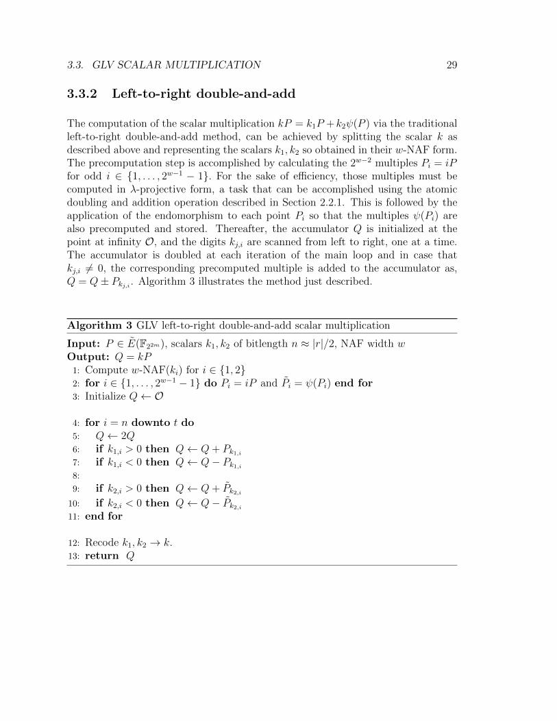
3.3.2 Left-to-right double-and-add
The computation of the scalar multiplication kP = k1P +k2ψ(P ) via the traditionalleft-to-right double-and-add method, can be achieved by splitting the scalar k asdescribed above and representing the scalars k1, k2 so obtained in their w-NAF form.The precomputation step is accomplished by calculating the 2w−2 multiples Pi = iPfor odd i ∈ {1, . . . , 2w−1 − 1}. For the sake of efficiency, those multiples must becomputed in λ-projective form, a task that can be accomplished using the atomicdoubling and addition operation described in Section 2.2.1. This is followed by theapplication of the endomorphism to each point Pi so that the multiples ψ(Pi) arealso precomputed and stored. Thereafter, the accumulator Q is initialized at thepoint at infinity O, and the digits kj,i are scanned from left to right, one at a time.The accumulator is doubled at each iteration of the main loop and in case thatkj,i 6= 0, the corresponding precomputed multiple is added to the accumulator as,Q = Q± Pkj,i . Algorithm 3 illustrates the method just described.
Algorithm 3 GLV left-to-right double-and-add scalar multiplication
Input: P ∈ E(F22m), scalars k1, k2 of bitlength n ≈ |r|/2, NAF width wOutput: Q = kP
1: Compute w-NAF(ki) for i ∈ {1, 2}2: for i ∈ {1, . . . , 2w−1 − 1} do Pi = iP and Pi = ψ(Pi) end for3: Initialize Q← O
4: for i = n downto t do5: Q← 2Q6: if k1,i > 0 then Q← Q+ Pk1,i7: if k1,i < 0 then Q← Q− Pk1,i8:
9: if k2,i > 0 then Q← Q+ Pk2,i10: if k2,i < 0 then Q← Q− Pk2,i11: end for
12: Recode k1, k2 → k.13: return Q
30 CHAPTER 3. GALBRAITH-LIN-SCOTT CURVES
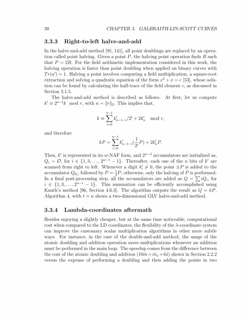
3.3.3 Right-to-left halve-and-add
In the halve-and-add method [95, 141], all point doublings are replaced by an opera-tion called point halving. Given a point P , the halving point operation finds R suchthat P = 2R. For the field arithmetic implementation considered in this work, thehalving operation is faster than point doubling when applied on binary curves withTr(a′) = 1. Halving a point involves computing a field multiplication, a square-rootextraction and solving a quadratic equation of the form x2 + x = c [53], whose solu-tion can be found by calculating the half-trace of the field element c, as discussed inSection 3.1.5.
The halve-and-add method is described as follows. At first, let us computek′ ≡ 2n−1k mod r, with n = ‖r‖2. This implies that,
k ≡n−1∑i=0
k′n−1−i/2i + 2k′n mod r,
and therefore
kP =n−1∑i=0
k′n−1−i(1
2iP ) + 2k′nP.
Then, k′ is represented in its w-NAF form, and 2w−2 accumulators are initialized as,Qi = O, for i ∈ {1, 3, . . ., 2w−1 − 1}. Thereafter, each one of the n bits of k′ arescanned from right to left. Whenever a digit k′i 6= 0, the point ±P is added to theaccumulator Qk′i
, followed by P = 12P ; otherwise, only the halving of P is performed.
In a final post-processing step, all the accumulators are added as Q =∑iQi, for
i ∈ {1, 3, . . . , 2w−1 − 1}. This summation can be efficiently accomplished usingKnuth’s method [96, Section 4.6.3]. The algorithm outputs the result as Q = kP .Algorithm 4, with t = n shows a two-dimensional GLV halve-and-add method.
3.3.4 Lambda-coordinates aftermath
Besides enjoying a slightly cheaper, but at the same time noticeable, computationalcost when compared to the LD coordinates, the flexibility of the λ-coordinate systemcan improve the customary scalar multiplication algorithms in other more subtleways. For instance, in the case of the double-and-add method, the usage of theatomic doubling and addition operation saves multiplications whenever an additionmust be performed in the main loop. The speedup comes from the difference betweenthe cost of the atomic doubling and addition (10m+ ma + 6s) shown in Section 2.2.2versus the expense of performing a doubling and then adding the points in two

3.3. GLV SCALAR MULTIPLICATION 31
Algorithm 4 GLV right-to-left halve-and-add scalar multiplication
Input: P ∈ E(F22m), scalars k1, k2 of bitlength n ≈ |r|/2, NAF width wOutput: Q = kP
1: Calculate w-NAF(ki) for i ∈ {1, 2}2: for i ∈ {1, . . . , 2w−1 − 1} do Initialize Qi ← O end for
3: for i = n− 1 downto 0 do4: if k1,i > 0 then Qk1,i ← Qk1,i + P5: if k1,i < 0 then Qk1,i ← Qk1,i − P6:
7: if k2,i > 0 then Qk2,i ← Qk2,i + ψ(P )8: if k2,i < 0 then Qk2,i ← Qk2,i − ψ(P )9: P ← P/2
10: end for
11: Q←∑
i∈{1,...,2w−1−1} iQi
12: Recode k1, k2 → k, if necessary.13: return Q
separate steps (12m+ ma + 6s). To see the overall impact of this saving in say, theGLV double-and-add method, one has to calculate the probabilities of one, two orno additions in a loop iteration.
Basically, three cases can occur in the 2-GLV double-and-add main loop. Thefirst one, when the digits of both scalars k1, k2 equal zero, we just perform a pointdoubling (D) in the accumulator. The second one, when both scalar digits aredifferent from zero, we have to double the accumulator and sum two points. In thiscase, we perform one doubling and addition (DA) followed by a mixed addition (A).Finally, it is possible that just one scalar has its digit different from zero. Here, wedouble the accumulator and add a point, which can be done with only one doubling-and-addition operation.
Then, as the nonzero bit distributions in the scalars represented by the w-NAFare independent, we have for the first case,
Pr[k1,i = 0 ∧ k2,i = 0] =w2
(w + 1)2, for i ∈ {0, . . . , n− 1}.
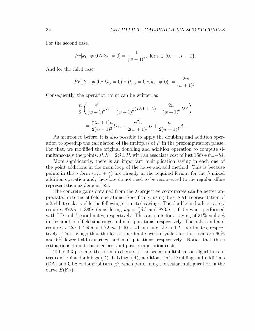
32 CHAPTER 3. GALBRAITH-LIN-SCOTT CURVES
For the second case,
Pr[k1,i 6= 0 ∧ k2,i 6= 0] =1
(w + 1)2, for i ∈ {0, . . . , n− 1}.
And for the third case,
Pr[(k1,i 6= 0 ∧ k2,i = 0) ∨ (k1,i = 0 ∧ k2,i 6= 0)] =2w
(w + 1)2.
Consequently, the operation count can be written as
n
2
(w2
(w + 1)2D +
1
(w + 1)2(DA+ A) +
2w
(w + 1)2DA
)
=(2w + 1)n
2(w + 1)2DA+
w2n
2(w + 1)2D +
n
2(w + 1)2A.
As mentioned before, it is also possible to apply the doubling and addition oper-ation to speedup the calculation of the multiples of P in the precomputation phase.For that, we modified the original doubling and addition operation to compute si-multaneously the points, R, S = 2Q±P , with an associate cost of just 16m+ma+8s.
More significantly, there is an important multiplication saving in each one ofthe point additions in the main loop of the halve-and-add method. This is becausepoints in the λ-form (x, x + y
x) are already in the required format for the λ-mixed
addition operation and, therefore do not need to be reconverted to the regular affinerepresentation as done in [53].
The concrete gains obtained from the λ-projective coordinates can be better ap-preciated in terms of field operations. Specifically, using the 4-NAF representation ofa 254-bit scalar yields the following estimated savings. The double-and-add strategyrequires 872m + 889s (considering mb = 2
3m) and 823m + 610s when performed
with LD and λ-coordinates, respectively. This amounts for a saving of 31% and 5%in the number of field squarings and multiplications, respectively. The halve-and-addrequires 772m + 255s and 721m + 101s when using LD and λ-coordinates, respec-tively. The savings that the latter coordinate system yields for this case are 60%and 6% fewer field squarings and multiplications, respectively. Notice that theseestimations do not consider pre- and post-computation costs.
Table 3.3 presents the estimated costs of the scalar multiplication algorithms interms of point doublings (D), halvings (H), additions (A), Doubling and additions(DA) and GLS endomorphisms (ψ) when performing the scalar multiplication in thecurve E(Fq2).
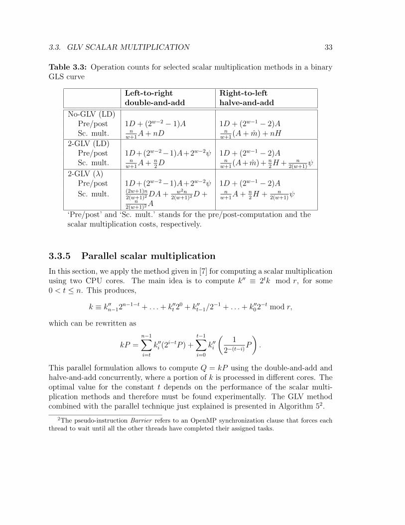
3.3. GLV SCALAR MULTIPLICATION 33
Table 3.3: Operation counts for selected scalar multiplication methods in a binaryGLS curve
Left-to-rightdouble-and-add
Right-to-lefthalve-and-add
No-GLV (LD)Pre/post 1D + (2w−2 − 1)A 1D + (2w−1 − 2)ASc. mult. n
w+1A+ nD n
w+1(A+ m) + nH
2-GLV (LD)Pre/post 1D+(2w−2−1)A+2w−2ψ 1D + (2w−1 − 2)ASc. mult. n
w+1A+ n
2D n
w+1(A+ m) + n
2H+ n
2(w+1)ψ
2-GLV (λ)Pre/post 1D+(2w−2−1)A+2w−2ψ 1D + (2w−1 − 2)A
Sc. mult. (2w+1)n2(w+1)2
DA+ w2n2(w+1)2
D +n
2(w+1)2A
nw+1
A+ n2H + n
2(w+1)ψ
‘Pre/post’ and ‘Sc. mult.’ stands for the pre/post-computation and thescalar multiplication costs, respectively.
3.3.5 Parallel scalar multiplication
In this section, we apply the method given in [7] for computing a scalar multiplicationusing two CPU cores. The main idea is to compute k′′ ≡ 2tk mod r, for some0 < t ≤ n. This produces,
k ≡ k′′n−12n−1−t + . . .+ k′′t 20 + k′′t−1/2−1 + . . .+ k′′02−t mod r,
which can be rewritten as
kP =n−1∑i=t
k′′i (2i−tP ) +t−1∑i=0
k′′i
(1
2−(t−i)P
).
This parallel formulation allows to compute Q = kP using the double-and-add andhalve-and-add concurrently, where a portion of k is processed in different cores. Theoptimal value for the constant t depends on the performance of the scalar multi-plication methods and therefore must be found experimentally. The GLV methodcombined with the parallel technique just explained is presented in Algorithm 52.
2The pseudo-instruction Barrier refers to an OpenMP synchronization clause that forces eachthread to wait until all the other threads have completed their assigned tasks.
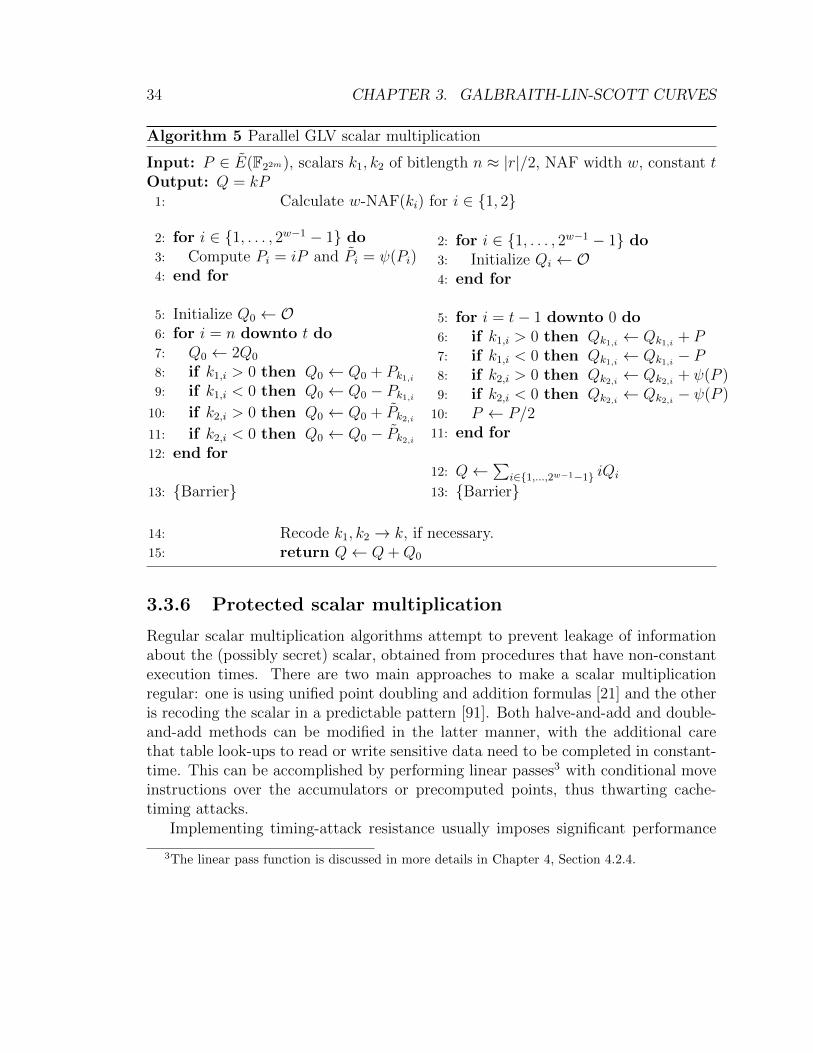
34 CHAPTER 3. GALBRAITH-LIN-SCOTT CURVES
Algorithm 5 Parallel GLV scalar multiplication
Input: P ∈ E(F22m), scalars k1, k2 of bitlength n ≈ |r|/2, NAF width w, constant tOutput: Q = kP
1: Calculate w-NAF(ki) for i ∈ {1, 2}
2: for i ∈ {1, . . . , 2w−1 − 1} do3: Compute Pi = iP and Pi = ψ(Pi)4: end for
5: Initialize Q0 ← O6: for i = n downto t do7: Q0 ← 2Q0
8: if k1,i > 0 then Q0 ← Q0 + Pk1,i9: if k1,i < 0 then Q0 ← Q0 − Pk1,i
10: if k2,i > 0 then Q0 ← Q0 + Pk2,i11: if k2,i < 0 then Q0 ← Q0 − Pk2,i12: end for
13: {Barrier}
2: for i ∈ {1, . . . , 2w−1 − 1} do3: Initialize Qi ← O4: end for
5: for i = t− 1 downto 0 do6: if k1,i > 0 then Qk1,i ← Qk1,i + P7: if k1,i < 0 then Qk1,i ← Qk1,i − P8: if k2,i > 0 then Qk2,i ← Qk2,i + ψ(P )9: if k2,i < 0 then Qk2,i ← Qk2,i − ψ(P )
10: P ← P/211: end for
12: Q←∑
i∈{1,...,2w−1−1} iQi
13: {Barrier}
14: Recode k1, k2 → k, if necessary.15: return Q← Q+Q0
3.3.6 Protected scalar multiplication
Regular scalar multiplication algorithms attempt to prevent leakage of informationabout the (possibly secret) scalar, obtained from procedures that have non-constantexecution times. There are two main approaches to make a scalar multiplicationregular: one is using unified point doubling and addition formulas [21] and the otheris recoding the scalar in a predictable pattern [91]. Both halve-and-add and double-and-add methods can be modified in the latter manner, with the additional carethat table look-ups to read or write sensitive data need to be completed in constant-time. This can be accomplished by performing linear passes3 with conditional moveinstructions over the accumulators or precomputed points, thus thwarting cache-timing attacks.
Implementing timing-attack resistance usually imposes significant performance
3The linear pass function is discussed in more details in Chapter 4, Section 4.2.4.
3.3. GLV SCALAR MULTIPLICATION 35
penalties. For example, the density of regular recodings ( 1w−1
) is considerably lowerthan w-NAF and the access to precomputed data becomes more expensive due tothe linear passes. Efficiently computing a point halving in constant time is speciallychallenging, since the fastest methods for half-trace computation require considerableamounts of memory. This requirement can be relaxed if we assume that the basepoints are public information and available to the attacker. Notice however that thisis a reasonable assumption in most protocols based on elliptic curves, but there areexceptions [35]. In any case, performing linear passes to read and store each one of the2w−2 accumulators used in the halve-and-add procedure discussed in Section 3.3.3,impose a significant impact performance at every point addition.
Because of the above rationale, doubling-based methods seem to be a morepromising option for protected implementations. Somewhat surprisingly, the reg-ular recoding method combined with λ-coordinates admits an atomic formula forcomputing mixed addition plus doubling-and-addition as 2Q+Pi +Pj with a cost of17m+ma+8s, saving one multiplication compared to performing the additions sepa-rately. Reading the points Pi, Pj can also be optimized by performing a single linearpass over the precomputed table. These optimizations alone are enough to compen-sate the performance gap between point doubling and point halving computationsto be presented in the next section.
The approach for protected scalar multiplication is shown in Algorithm 6. Inthis procedure, the scalar k is decomposed into subscalars k1, k2 before the mainloop. Because the regular recoding requires the input scalar to be odd, we modifiedslightly the GLV recoding algorithm to produce k2 always odd, with at most one extrapoint addition needed to correct the result at the end. This is actually faster thangenerating random and possibly even k1, k2 for reconstructing k, because otherwisetwo point additions would be needed for correction. These extra point additionsmust always be performed for satisfying constant-time execution, but conditionalmove instructions can be used to eliminate incorrect results.
3.3.7 Results and discussion
Our library targets the Intel Sandy Bridge processor family. This multi-core micro-architecture supports carry-less multiplications, the SSE set of instructions [128]that operates on 128-bit registers and the AVX extension [51], which provides SIMDinstructions in a three-operand format. However, our code can be easily adaptedto any architecture that supports the aforementioned features. The benchmarkingwas run on an Intel Xeon E31270 3.4GHz and on an Intel Core i5 3570 3.4GHzwith the TurboBoost and the HyperThreading technologies disabled. The code was

36 CHAPTER 3. GALBRAITH-LIN-SCOTT CURVES
Algorithm 6 Protected scalar multiplication
Input: P ∈ E(F22m) of order r, k ∈ Zr, NAF width wOutput: Q = kP
1: Decompose k into k1, k2, with k2 always odd.2: c← 1− (k1 mod 2)3: k1 ← k1 + c4: Compute width-w length-l regular recodings of k1, k2.
5: for i ∈ {1, . . . , 2w−1 − 1} do Compute Pi = iP end for
6: Q← Pk1,l−1+ ψ(Pk2,l−1
)7: for i = l − 2 downto 0 do8: Q← 2w−2Q9: Perform a linear pass to recover Pk1,i , Pk2,i .
10: Q← 2Q+ Pk1,i + ψ(Pk2,i)11: end for
12: return Q← Q− cP
implemented in the C programming language with intrinsics for vector instructions,compiled with GCC 4.8.1 and executed on 64-bit Linux. Experiments with theICC 13.0 were also carried out and generated similar results. For that reason, weabstain from presenting timings for that compiler. Also, portions of the code criticalfor timing-attack resistance (linear passes over precomputed tables, for example),were implemented in Assembly language to prevent undue manipulation by a code-optimizing compiler.
GLS curve parameters
The main parameters of the GLS curve implemented in this chapter are presentedbelow.
Let q = 2m, with m = 127. The towering of the fields Fq and its quadraticextension Fq2 ∼= Fq[u]/(g(u)) are constructed by means of the irreducible trinomialsf(x) = x127 + x63 + 1 and g(u) = u2 + u+ 1, respectively. Let
E/Fq : y2 + xy = x3 + ax2 + b,
with a, b ∈ Fq, be a binary elliptic curve and define the quadratic twist of E as the
3.3. GLV SCALAR MULTIPLICATION 37
Galbraith-Lin-Scott elliptic curve
E/Fq2 : y2 + xy = x3 + a′x2 + b,
with a′ ∈ Fq2 such that Tr(a′) = 1. Given #E(Fq) = q + 1 − t, it follows that
#E(Fq2) = (q−1)2 + t2 where t is the trace of Frobenius of the curve E. We selected
a curve such that #E(Fq2) = h · r, where h = 2 and r is a 253-bit prime number.
In this work, the binary GLS elliptic curve E(Fq2) was defined with the followingparameters
• a′ = u.
• b ∈ Fq is a degree-126 binary polynomial that can be represented in hexadecimalformat as, b = 0x59C8202CB9E6E0AE2E6D944FA54DE7E5.
• The 253-bit prime order r of the main subgroup of Ea′,b(Fq2) is,
r =0x1FFFFFFFFFFFFFFFFFFFFFFFFFFFFFFF
DAC40D1195270779877DABA2A44750A5.
• The base point P = (xp, λp) of order r specified in λ−affine coordinates is,
xp = 0x203B6A93395E0432344038B63FBA32DE
+ 0x78E51FD0C310696D5396E0681AA10E0D · u,λp = 0x5BD7653482085F55DEB59C6137074B50
+ 0x7F90D98B1589A17F24568FA5A1033946 · u.
Field and elliptic curve arithmetic timings
Table 3.4 shows that the quadratic field arithmetic can handle the base field elementswith considerable efficiency. Field inversion, squaring and square-root, as well asthe half-trace computational costs are just 1.27, 1.44, 1.87 and 1.43 times higherthan their corresponding base field operations, respectively. Field multiplication inthe quadratic field can be accomplished at a cost of about 2.23 times base fieldmultiplications, which is significantly better than the theoretical Karatsuba ratio ofthree.
The lazy reduction technique was employed to optimize the λ-coordinate formu-las. Nevertheless, experimental results showed us that this method should be usedwith caution. Extra savings were obtained by considering the separate case of per-forming mixed addition where the two points have their Z coordinate equal to one
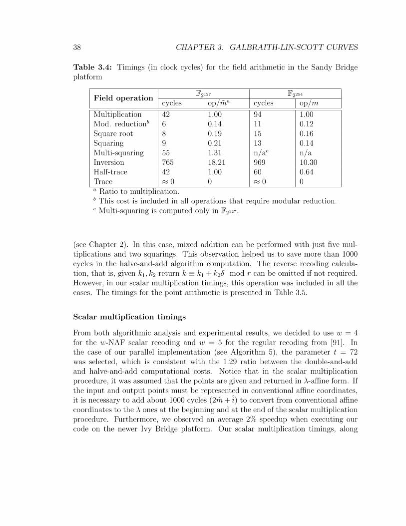
38 CHAPTER 3. GALBRAITH-LIN-SCOTT CURVES
Table 3.4: Timings (in clock cycles) for the field arithmetic in the Sandy Bridgeplatform
Field operationF2127 F2254
cycles op/ma cycles op/m
Multiplication 42 1.00 94 1.00Mod. reductionb 6 0.14 11 0.12Square root 8 0.19 15 0.16Squaring 9 0.21 13 0.14Multi-squaring 55 1.31 n/ac n/aInversion 765 18.21 969 10.30Half-trace 42 1.00 60 0.64Trace ≈ 0 0 ≈ 0 0a Ratio to multiplication.b This cost is included in all operations that require modular reduction.c Multi-squaring is computed only in F2127 .
(see Chapter 2). In this case, mixed addition can be performed with just five mul-tiplications and two squarings. This observation helped us to save more than 1000cycles in the halve-and-add algorithm computation. The reverse recoding calcula-tion, that is, given k1, k2 return k ≡ k1 + k2δ mod r can be omitted if not required.However, in our scalar multiplication timings, this operation was included in all thecases. The timings for the point arithmetic is presented in Table 3.5.
Scalar multiplication timings
From both algorithmic analysis and experimental results, we decided to use w = 4for the w-NAF scalar recoding and w = 5 for the regular recoding from [91]. Inthe case of our parallel implementation (see Algorithm 5), the parameter t = 72was selected, which is consistent with the 1.29 ratio between the double-and-addand halve-and-add computational costs. Notice that in the scalar multiplicationprocedure, it was assumed that the points are given and returned in λ-affine form. Ifthe input and output points must be represented in conventional affine coordinates,it is necessary to add about 1000 cycles (2m+ i) to convert from conventional affinecoordinates to the λ ones at the beginning and at the end of the scalar multiplicationprocedure. Furthermore, we observed an average 2% speedup when executing ourcode on the newer Ivy Bridge platform. Our scalar multiplication timings, along

3.3. GLV SCALAR MULTIPLICATION 39
Table 3.5: Timings (in clock cycles) for the point arithmetic in the Sandy Bridgeplatform
Elliptic Curve GLS E/F2254
operation cycles op/M
Doubling 450 4.79Full addition 1,102 11.72Mixed addition 812 8.64Doubling and addition 1,063 11.30Halving 233 2.48No-GLV 4-NAF recoding 1,540 16.382-GLV 4-NAF recoding 918 9.76Reverse recoding 396 4.21
with the state-of-the-art implementations, are presented in Table 3.6.
Comparison to related work
Our single-core 4-NAF 2-dimensional GLV implementation achieves 69,500 clock cy-cles with the halve-and-add method. This result is 20% and 30% faster than the bestimplementations of point multiplication at the 128-bit security level over prime [50]and binary curves [9], respectively. Furthermore, our two-core parallel implementa-tion using the GLV technique combined with the halve-and-add and double-and-addmethods takes 47,900 clock cycles, thus outperforming by 21% the timings reportedin [102] for a four-core parallel implementation. Also, the single and multi-core imple-mentations at the 112-bit security level using Koblitz binary curves reported in [148]outperforms our code by just 2% and 3%, respectively. Finally, our single-core pro-tected multiplication is 16% faster than [102], 4% faster than [27] and 16% slowerthan the current speed record on prime curves [50], but sets a new speed record forbinary curves with an improvement of 49% compared to the previous one [148].
A field multiplication comparative
Trying to have a fair comparison that attenuates the diversity of curves, methodsand technologies, Table 3.7 compares the estimated number of field multiplicationsrequired by implementations that represent the state-of-the-art of unprotected im-plementations of scalar multiplication computations.
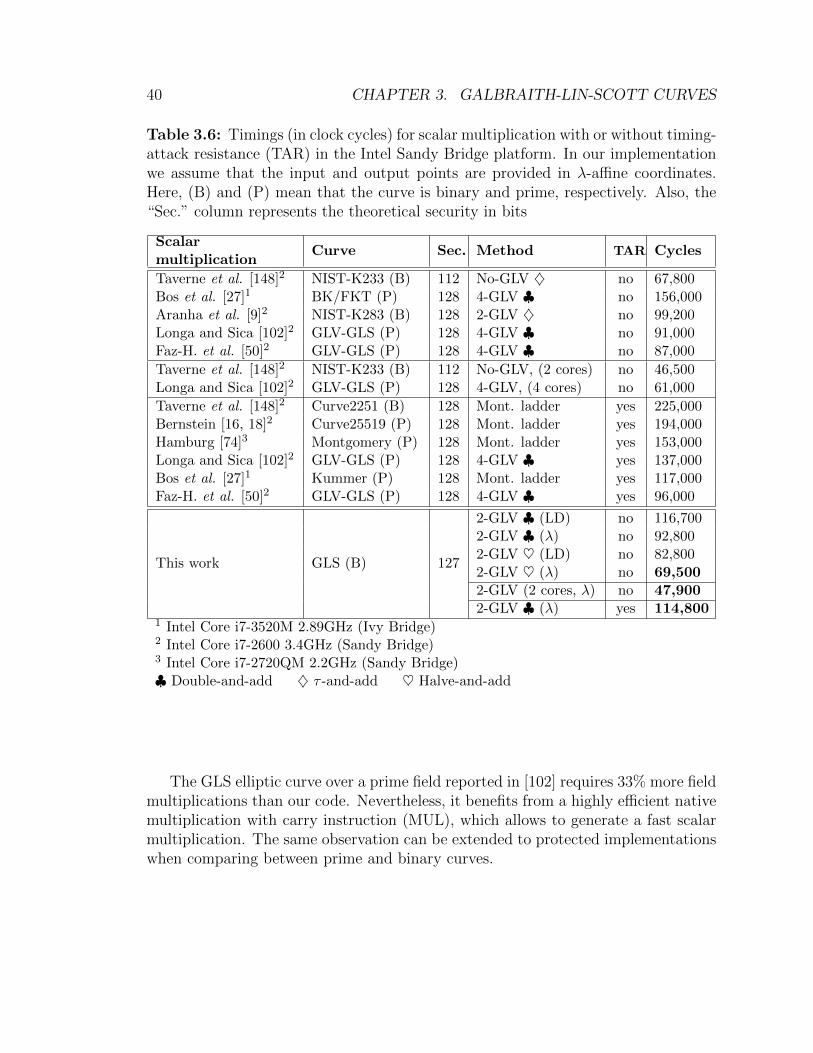
40 CHAPTER 3. GALBRAITH-LIN-SCOTT CURVES
Table 3.6: Timings (in clock cycles) for scalar multiplication with or without timing-attack resistance (TAR) in the Intel Sandy Bridge platform. In our implementationwe assume that the input and output points are provided in λ-affine coordinates.Here, (B) and (P) mean that the curve is binary and prime, respectively. Also, the“Sec.” column represents the theoretical security in bits
Scalarmultiplication
Curve Sec. Method TAR Cycles
Taverne et al. [148]2 NIST-K233 (B) 112 No-GLV ♦ no 67,800Bos et al. [27]1 BK/FKT (P) 128 4-GLV ♣ no 156,000Aranha et al. [9]2 NIST-K283 (B) 128 2-GLV ♦ no 99,200Longa and Sica [102]2 GLV-GLS (P) 128 4-GLV ♣ no 91,000Faz-H. et al. [50]2 GLV-GLS (P) 128 4-GLV ♣ no 87,000
Taverne et al. [148]2 NIST-K233 (B) 112 No-GLV, (2 cores) no 46,500Longa and Sica [102]2 GLV-GLS (P) 128 4-GLV, (4 cores) no 61,000
Taverne et al. [148]2 Curve2251 (B) 128 Mont. ladder yes 225,000Bernstein [16, 18]2 Curve25519 (P) 128 Mont. ladder yes 194,000Hamburg [74]3 Montgomery (P) 128 Mont. ladder yes 153,000Longa and Sica [102]2 GLV-GLS (P) 128 4-GLV ♣ yes 137,000Bos et al. [27]1 Kummer (P) 128 Mont. ladder yes 117,000Faz-H. et al. [50]2 GLV-GLS (P) 128 4-GLV ♣ yes 96,000
This work GLS (B) 127
2-GLV ♣ (LD) no 116,7002-GLV ♣ (λ) no 92,8002-GLV ♥ (LD) no 82,8002-GLV ♥ (λ) no 69,5002-GLV (2 cores, λ) no 47,9002-GLV ♣ (λ) yes 114,800
1 Intel Core i7-3520M 2.89GHz (Ivy Bridge)2 Intel Core i7-2600 3.4GHz (Sandy Bridge)3 Intel Core i7-2720QM 2.2GHz (Sandy Bridge)♣ Double-and-add ♦ τ -and-add ♥ Halve-and-add
The GLS elliptic curve over a prime field reported in [102] requires 33% more fieldmultiplications than our code. Nevertheless, it benefits from a highly efficient nativemultiplication with carry instruction (MUL), which allows to generate a fast scalarmultiplication. The same observation can be extended to protected implementationswhen comparing between prime and binary curves.
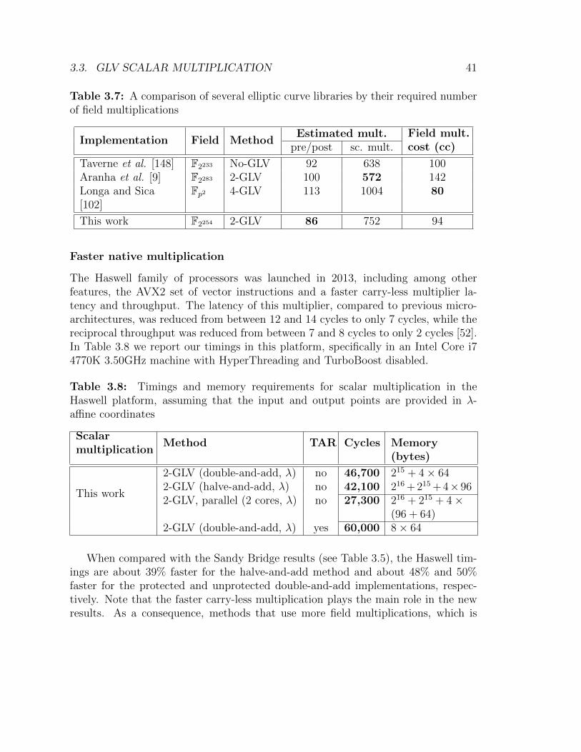
3.3. GLV SCALAR MULTIPLICATION 41
Table 3.7: A comparison of several elliptic curve libraries by their required numberof field multiplications
Implementation Field MethodEstimated mult. Field mult.
cost (cc)pre/post sc. mult.
Taverne et al. [148] F2233 No-GLV 92 638 100Aranha et al. [9] F2283 2-GLV 100 572 142Longa and Sica[102]
Fp2 4-GLV 113 1004 80
This work F2254 2-GLV 86 752 94
Faster native multiplication
The Haswell family of processors was launched in 2013, including among otherfeatures, the AVX2 set of vector instructions and a faster carry-less multiplier la-tency and throughput. The latency of this multiplier, compared to previous micro-architectures, was reduced from between 12 and 14 cycles to only 7 cycles, while thereciprocal throughput was reduced from between 7 and 8 cycles to only 2 cycles [52].In Table 3.8 we report our timings in this platform, specifically in an Intel Core i74770K 3.50GHz machine with HyperThreading and TurboBoost disabled.
Table 3.8: Timings and memory requirements for scalar multiplication in theHaswell platform, assuming that the input and output points are provided in λ-affine coordinates
Scalarmultiplication
Method TAR Cycles Memory(bytes)
This work
2-GLV (double-and-add, λ) no 46,700 215 + 4× 642-GLV (halve-and-add, λ) no 42,100 216 + 215 + 4×962-GLV, parallel (2 cores, λ) no 27,300 216 + 215 + 4×
(96 + 64)2-GLV (double-and-add, λ) yes 60,000 8× 64
When compared with the Sandy Bridge results (see Table 3.5), the Haswell tim-ings are about 39% faster for the halve-and-add method and about 48% and 50%faster for the protected and unprotected double-and-add implementations, respec-tively. Note that the faster carry-less multiplication plays the main role in the newresults. As a consequence, methods that use more field multiplications, which is
42 CHAPTER 3. GALBRAITH-LIN-SCOTT CURVES
the case of the double-and-add, benefit the most. The competitiveness between thedouble-and-add and halve-and-add methods favors the parallel version, which canalmost achieve a two-factor speed-up. When executed in the Haswell platform, thetwo-core 2-GLV method is 43% faster than the Sandy Bridge timings.
Memory requirements
The library presented in this chapter is intended for its application in high-endplatforms where, typically, memory is an abundant resource. Accordingly, severalarithmetic operations aggressively use precomputed tables with the aim of achievinga faster computation than what could be obtained by a direct calculation.
In particular, the base field implementation of the half-trace operation, uses aprecomputed table of size 28 · dm
8e field elements. Using m = 128, this translates to
a 216-byte table. The faster field inverse implementation invokes four multi-squaringoperations, but the constant-time implementations uses slower consecutive squarings.Each one of these multi-squaring operations requires to precompute a table of size24 · dm
4e field elements, that translates to a table with a size of 213 bytes. Therefore,
the memory cost associated to the faster field inversion computation in our library isof 215 bytes. Finally, the halve-and-add scalar multiplication requires the storage of 4accumulators in projective coordinates; and the double-and-add scalar multiplicationrequires the storage of 4 and 8 multiples of the base point for the unprotected andprotected versions, respectively. A summary of the memory costs associated to thescalar multiplication algorithms presented in this work are reported in the last columnof Table 3.8.
3.4 Montgomery ladder scalar multiplication
In this part, we present new methods aimed to perform fast constant-time variable-base-point multiplication computation for GLS binary elliptic curves. We introduce anovel right-to-left variant of the classical Montgomery-Lopez-Dahab ladder algorithmpresented in [104], which efficiently adapted the original ladder idea introduced byPeter Montgomery in his 1987 landmark paper [114]. The new variant presentedin this chapter does not require point doublings, but instead, it uses the efficientpoint halving operation available on binary elliptic curves. In contrast with thealgorithm presented in [104] that does not admit the benefit of precomputed tables,our proposed variant can take advantage of this technique, a feature that could bevaluable for the fixed-base-point multiplication scenario. Moreover, we show thatour new right-to-left Montgomery ladder formulation can be nicely combined with
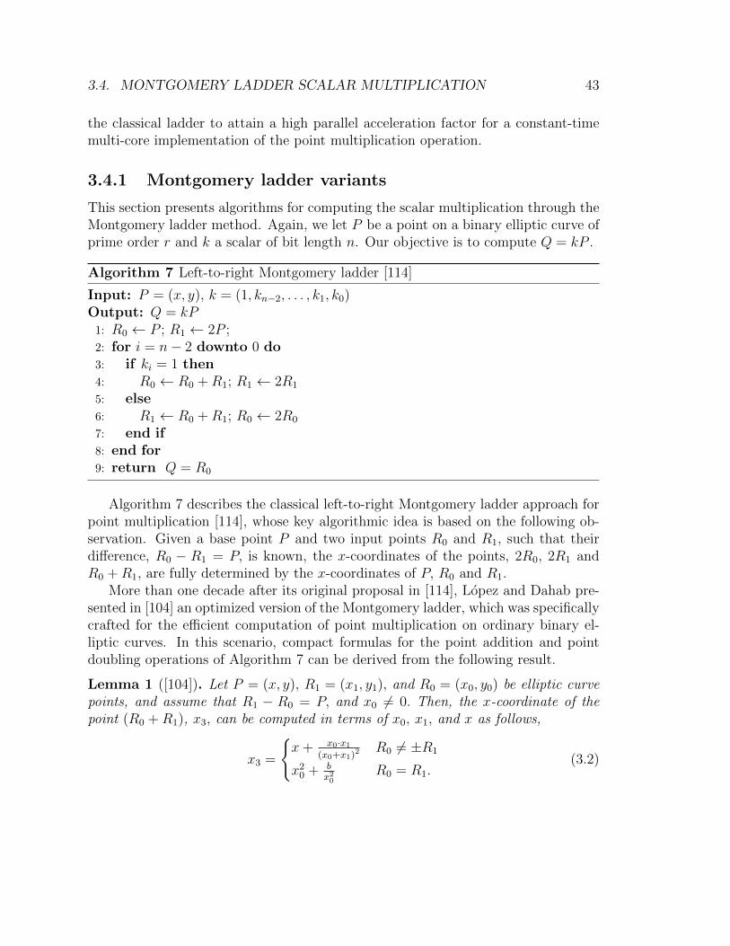
3.4. MONTGOMERY LADDER SCALAR MULTIPLICATION 43
the classical ladder to attain a high parallel acceleration factor for a constant-timemulti-core implementation of the point multiplication operation.
3.4.1 Montgomery ladder variants
This section presents algorithms for computing the scalar multiplication through theMontgomery ladder method. Again, we let P be a point on a binary elliptic curve ofprime order r and k a scalar of bit length n. Our objective is to compute Q = kP .
Algorithm 7 Left-to-right Montgomery ladder [114]
Input: P = (x, y), k = (1, kn−2, . . . , k1, k0)Output: Q = kP
1: R0 ← P ; R1 ← 2P ;2: for i = n− 2 downto 0 do3: if ki = 1 then4: R0 ← R0 +R1; R1 ← 2R1
5: else6: R1 ← R0 +R1; R0 ← 2R0
7: end if8: end for9: return Q = R0
Algorithm 7 describes the classical left-to-right Montgomery ladder approach forpoint multiplication [114], whose key algorithmic idea is based on the following ob-servation. Given a base point P and two input points R0 and R1, such that theirdifference, R0 − R1 = P, is known, the x-coordinates of the points, 2R0, 2R1 andR0 +R1, are fully determined by the x-coordinates of P, R0 and R1.
More than one decade after its original proposal in [114], Lopez and Dahab pre-sented in [104] an optimized version of the Montgomery ladder, which was specificallycrafted for the efficient computation of point multiplication on ordinary binary el-liptic curves. In this scenario, compact formulas for the point addition and pointdoubling operations of Algorithm 7 can be derived from the following result.
Lemma 1 ([104]). Let P = (x, y), R1 = (x1, y1), and R0 = (x0, y0) be elliptic curvepoints, and assume that R1 − R0 = P, and x0 6= 0. Then, the x-coordinate of thepoint (R0 +R1), x3, can be computed in terms of x0, x1, and x as follows,
x3 =
{x+ x0·x1
(x0+x1)2R0 6= ±R1
x20 + b
x20R0 = R1.
(3.2)
44 CHAPTER 3. GALBRAITH-LIN-SCOTT CURVES
Moreover, the y-coordinate of R0 can be expressed in terms of P, and the x-coordinatesof R0, R1 as,
y0 = x−1(x0 + x)[(x0 + x)(x1 + x) + x2 + y
]+ y. (3.3)
Let us denote the projective representation of the points R0, R1 and R0 + R1,without considering their y-coordinates as, R0 = (X0,−, Z0), R1 = (X1,−, Z1) andR0 +R1 = (X3,−, Z3). Then, for the case R0 = R1, Lemma 1 implies,{
X3 = X40 + b · Z4
0
Z3 = X20 · Z2
0 .(3.4)
Furthermore, for the case R0 6= ±R1, one has that,{Z3 = (X0 · Z1 +X1 · Z0)2
X3 = x · Z3 + (X0 · Z1) · (X1 · Z0).(3.5)
From Equations (3.4) and (3.5) it follows that the computational cost of eachladder step in Algorithm 7 is 5 multiplications, 1 multiplication by the curve param-eter b, 4 or 5 squarings4 and 3 additions over the binary extension field where theelliptic curve has been defined.
In the rest of this section, we will present a novel right-to-left formulation of theclassical Montgomery ladder.
Right-to-left double-and-add Montgomery-LD ladder
Algorithm 8 presents a right-to-left version of the classical Montgomery ladder pro-cedure. At the end of the i-th iteration, the points in the variables R0, R1 areR0 = 2i+1P and R1 = `P + P
2, where ` is the integer represented by the i rightmost
bits of the scalar k. The variable R2 maintains the relationship, R2 = R0 − R1
from the initialization (step 1), until the execution of the last iteration of the mainloop (steps 2-9). This comes from the fact that at each iteration, if ki = 1, thenthe difference R0 − R1 remains unchanged. If otherwise, ki = 0, then both R2 andR0 are updated with their respective original values plus R0, which ensures thatR2 = R0−R1, still holds. Notice however that although the difference R2 = R0−R1
is known, it may vary throughout the iterations.As stated in Lemma 1, the point additions of steps 4 and 6 in Algorithm 8 can
be computed using the x-coordinates of the points R0, R1 and R2, according to the
4Either b = 1 or√b is precomputed. Formula (3.4) can also be computed as Z3 = (X0 · Z0)2
and X3 = (X20 +√b · Z2
0 )2
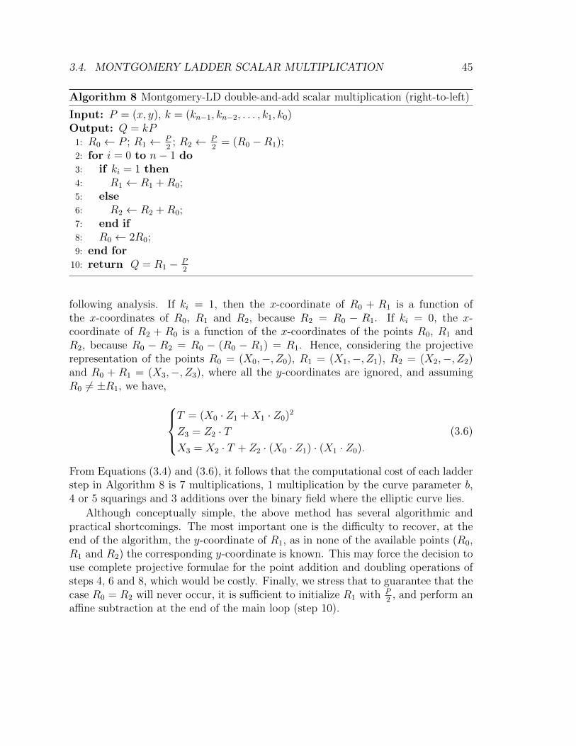
3.4. MONTGOMERY LADDER SCALAR MULTIPLICATION 45
Algorithm 8 Montgomery-LD double-and-add scalar multiplication (right-to-left)
Input: P = (x, y), k = (kn−1, kn−2, . . . , k1, k0)Output: Q = kP
1: R0 ← P ; R1 ← P2
; R2 ← P2
= (R0 −R1);2: for i = 0 to n− 1 do3: if ki = 1 then4: R1 ← R1 +R0;5: else6: R2 ← R2 +R0;7: end if8: R0 ← 2R0;9: end for
10: return Q = R1 − P2
following analysis. If ki = 1, then the x-coordinate of R0 + R1 is a function ofthe x-coordinates of R0, R1 and R2, because R2 = R0 − R1. If ki = 0, the x-coordinate of R2 + R0 is a function of the x-coordinates of the points R0, R1 andR2, because R0 − R2 = R0 − (R0 − R1) = R1. Hence, considering the projectiverepresentation of the points R0 = (X0,−, Z0), R1 = (X1,−, Z1), R2 = (X2,−, Z2)and R0 + R1 = (X3,−, Z3), where all the y-coordinates are ignored, and assumingR0 6= ±R1, we have,
T = (X0 · Z1 +X1 · Z0)2
Z3 = Z2 · TX3 = X2 · T + Z2 · (X0 · Z1) · (X1 · Z0).
(3.6)
From Equations (3.4) and (3.6), it follows that the computational cost of each ladderstep in Algorithm 8 is 7 multiplications, 1 multiplication by the curve parameter b,4 or 5 squarings and 3 additions over the binary field where the elliptic curve lies.
Although conceptually simple, the above method has several algorithmic andpractical shortcomings. The most important one is the difficulty to recover, at theend of the algorithm, the y-coordinate of R1, as in none of the available points (R0,R1 and R2) the corresponding y-coordinate is known. This may force the decision touse complete projective formulae for the point addition and doubling operations ofsteps 4, 6 and 8, which would be costly. Finally, we stress that to guarantee that thecase R0 = R2 will never occur, it is sufficient to initialize R1 with P
2, and perform an
affine subtraction at the end of the main loop (step 10).
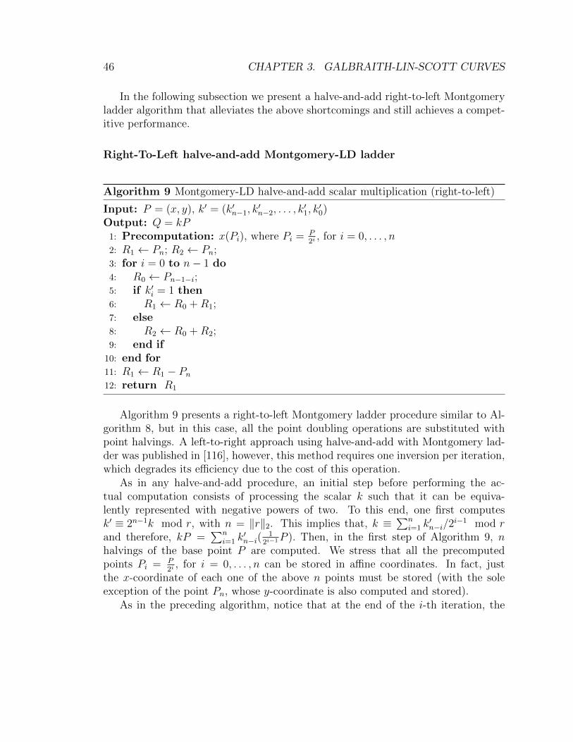
46 CHAPTER 3. GALBRAITH-LIN-SCOTT CURVES
In the following subsection we present a halve-and-add right-to-left Montgomeryladder algorithm that alleviates the above shortcomings and still achieves a compet-itive performance.
Right-To-Left halve-and-add Montgomery-LD ladder
Algorithm 9 Montgomery-LD halve-and-add scalar multiplication (right-to-left)
Input: P = (x, y), k′ = (k′n−1, k′n−2, . . . , k
′1, k′0)
Output: Q = kP1: Precomputation: x(Pi), where Pi = P
2i, for i = 0, . . . , n
2: R1 ← Pn; R2 ← Pn;3: for i = 0 to n− 1 do4: R0 ← Pn−1−i;5: if k′i = 1 then6: R1 ← R0 +R1;7: else8: R2 ← R0 +R2;9: end if
10: end for11: R1 ← R1 − Pn12: return R1
Algorithm 9 presents a right-to-left Montgomery ladder procedure similar to Al-gorithm 8, but in this case, all the point doubling operations are substituted withpoint halvings. A left-to-right approach using halve-and-add with Montgomery lad-der was published in [116], however, this method requires one inversion per iteration,which degrades its efficiency due to the cost of this operation.
As in any halve-and-add procedure, an initial step before performing the ac-tual computation consists of processing the scalar k such that it can be equiva-lently represented with negative powers of two. To this end, one first computesk′ ≡ 2n−1k mod r, with n = ‖r‖2. This implies that, k ≡
∑ni=1 k
′n−i/2
i−1 mod rand therefore, kP =
∑ni=1 k
′n−i(
12i−1P ). Then, in the first step of Algorithm 9, n
halvings of the base point P are computed. We stress that all the precomputedpoints Pi = P
2i, for i = 0, . . . , n can be stored in affine coordinates. In fact, just
the x-coordinate of each one of the above n points must be stored (with the soleexception of the point Pn, whose y-coordinate is also computed and stored).
As in the preceding algorithm, notice that at the end of the i-th iteration, the
3.4. MONTGOMERY LADDER SCALAR MULTIPLICATION 47
points in the variables R0, R1 are, R0 = P2n−i−1 , and R1 = `P +Pn, where in this case
` is the integer represented as ` =i∑
j=0
k′j2n−j
mod r. Notice also that the variable R2
maintains the relationship, R2 = R0−R1, until the execution of the last iteration ofthe main loop (steps 3-10). This comes from the fact that at each iteration, if ki = 1,then the difference R0 − R1 remains unchanged. If otherwise, ki = 0, then both R2
and R0 are updated with their respective original values plus R0, which ensures thatR2 = R0 −R1, still holds.
Since at every iteration, the values of the points R0, R1 and R0 − R1 are allknown, the compact point addition formula (3.6) can be used. In practice, thisis also possible because the y-coordinate of the output point kP can be readilyrecovered using Equation 3.3, along with the point 2P . Moreover, since the pointsin the precomputed table were generated using affine coordinates, it turns out thatthe z-coordinate of the point R0 is always 1 for all the iterations of the main loop.This simplifies (3.6) as,
T = (X0 · Z1 +X1)2
Z3 = Z2 · TX3 = X2 · T + Z2 · (X0 · Z1) · (X1).
(3.7)
Hence, the computational cost per iteration of Algorithm 9 is 5 multiplications, 1squaring, 2 additions and one point halving over the binary field where the ellipticcurve lies.
GLS Endomorphism The efficient computable endomorphism provided by theGLS curves can be used to implement the 2-GLV method on the Algorithm 9. Asa result, only n/2 point halving operations must be computed. Besides the speedimprovement, the 2-GLV method reduces to a half the number of precomputed pointsthat must be stored.
Multi-core Montgomery ladder
As proposed in [148], by properly recoding the scalar, one can efficiently computethe scalar multiplication in a multi-core environment. Specifically, given a scalar kof size n, we fix a constant t which establishes how many scalar bits will be processedby the double-and-add, and by the halve-and-add procedures. This is accomplishedby computing k′ = 2tk mod r, which yields
48 CHAPTER 3. GALBRAITH-LIN-SCOTT CURVES
k =k′02t
+k′1
2t−1+ · · ·+
k′t−1
21︸ ︷︷ ︸halve−and−add
+k′t20
+ 21k′t+1 + 22k′t+2 + · · ·+ 2(n−1)−tk′n−1︸ ︷︷ ︸double−and−add
.
In a two-core setting, it is straightforward to combine the left-to-right and right-to-left Montgomery ladder procedures of Algorithms 7 and 9, and distribute themto both cores. In this scenario, the number of necessary pre-computed halved pointsreduces to ∼ n
4.
In a four-core platform, we can apply the GLS endomorphism to the left-to-rightMontgomery ladder (Algorithm 7). Even though the GLV technique is ineffectivefor the classical Montgomery algorithm (due to the fact that we cannot share thepoint doublings between the base point and its endomorphism), the method permitsan efficient splitting of the algorithm workload into two cores. In this way, one canuse the first two cores for computing t-digits of the GLV subscalars k1 and k2 bymeans of Algorithm 9, while we allocate the other two cores to compute the rest ofthe scalar’s bits using Algorithm 7, as shown in Algorithm 10.
Given t4 the integer constant that establishes the workload of each algorithm,P ∈ E(Fq2), and the scalar k represented as k1 + k2 · δ using the GLS-GLV method,cores I and II are both responsible for computing bn
2c − t4 bits of the subscalars k1
and k2 using the Montgomery-LD double-and-add method. In turn, the cores IIIand IV , both compute t4 bits of k1 and k2 with the Montgomery-LD halve-and-addalgorithm. In the end, on a single core, it is necessary to add all the accumulatorsQi, for i = 0 . . . 3.
Cost comparison of Montgomery ladder variants
Table 3.9 shows the computational costs associated to the Montgomery ladder vari-ants described in this Section. The constants t2 and t4 represent the values of theparameter t chosen for the two- and four-core implementations, respectively.5 AllMontgomery ladder algorithms require a basic post-computation cost to retrieve they-coordinate, which demands ten multiplications, one squaring and one inversion.Due to the application of the GLV technique, the Montgomery-LD-2-GLV halve-and-add version (corresponding to Algorithm 9), requires some few extra operations,namely, the subtraction of a point and the addition of two accumulators, which isperformed using the Lopez-Dahab (LD) projective coordinate formulae. In the end,
5In our implementations, the values used for the parameters t2 and t4 ranged from 53 to 55.
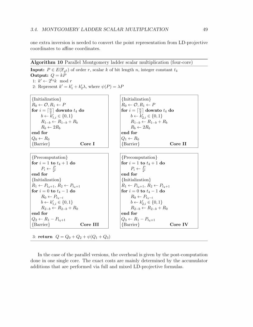
3.4. MONTGOMERY LADDER SCALAR MULTIPLICATION 49
one extra inversion is needed to convert the point representation from LD-projectivecoordinates to affine coordinates.
Algorithm 10 Parallel Montgomery ladder scalar multiplication (four-core)
Input: P ∈ E(Fq2) of order r, scalar k of bit length n, integer constant t4Output: Q = kP1: k′ ← 2t4k mod r2: Represent k′ = k′1 + k′2λ, where ψ(P ) = λP
{Initialization}R0 ← O, R1 ← Pfor i = dn2 e downto t4 do
b← k′1,i ∈ {0, 1}R1−b ← R1−b +RbRb ← 2Rb
end forQ0 ← R0
{Barrier} Core I
{Initialization}R0 ← O, R1 ← Pfor i = dn2 e downto t4 do
b← k′2,i ∈ {0, 1}R1−b ← R1−b +RbRb ← 2Rb
end forQ1 ← R0
{Barrier} Core II
{Precomputation}for i = 1 to t4 + 1 do
Pi ← P2i
end for{Initialization}R1 ← Pt4+1, R2 ← Pt4+1
for i = 0 to t4 − 1 doR0 ← Pt4−ib← k′1,i ∈ {0, 1}R2−b ← R2−b +R0
end forQ2 ← R1 − Pt4+1
{Barrier} Core III
{Precomputation}for i = 1 to t4 + 1 do
Pi ← P2i
end for{Initialization}R1 ← Pt4+1, R2 ← Pt4+1
for i = 0 to t4 − 1 doR0 ← Pt4−ib← k′2,i ∈ {0, 1}R2−b ← R2−b +R0
end forQ3 ← R1 − Pt4+1
{Barrier} Core IV
3: return Q = Q0 +Q2 + ψ(Q1 +Q3)
In the case of the parallel versions, the overhead is given by the post-computationdone in one single core. The exact costs are mainly determined by the accumulatoradditions that are performed via full and mixed LD-projective formulas.

50 CHAPTER 3. GALBRAITH-LIN-SCOTT CURVES
Table 3.9: Montgomery-LD algorithms cost comparison. In this table,m, ma, mb, s, i denote the following field operations: multiplication, multiplicationby the curve parameters a and b, squaring and inversion. The point halving opera-tion is denoted by H. The scalar bitlength is denoted as n
Method Cost
1-c
ore
Alg. 7: Montgomery-LD(double-and-add, left-to-right)
pre/post 10m+ 1s+ 1isc. mult. n(5m+ 1mb + 4s)
Alg. 9: Montgomery-LD-2-GLV(halve-and-add, right-to-left)
pre/post 48m+ 1ma + 13s+ 3isc. mult. (n
2+ 1)H + n(5m+ 1s)
2-c
ore
Montgomery-LD-2-GLV(double-and-add, left-to-right)
core Ipre/post 25m+ 1ma + 5s+ 2isc. mult. (n− t2)(5m+1mb+4s)
Montgomery-LD-2-GLV(halve-and-add, right-to-left)
core IIpre/post 46m+ 2ma + 12s+ 2isc. mult. ( t2
2+ 1)H + t2(5m+ 1s)
Overhead 15m+ 5s+ 1i
4-c
ore
Montgomery-LD-2-GLV(double-and-add, left-to-right)
cores pre/post 10m+ 1s+ 1iI & II sc. mult. (n
2− t4)(5m+1mb+4s)
Montgomery-LD-2-GLV(halve-and-add, right-to-left)
cores pre/post 16m+ 1ma + 4s+ 1iIII & IV sc. mult. ( t4
2+ 1)H + t4(5m+ 1s)
Overhead 34m+ 1ma + 12s+ 1i
3.4.2 Results and discussion
In this part, we discuss several implementation issues. We also present our ex-perimental results and we compare them against state-of-the-art protected pointmultiplication implementations at the 128-bit security level.
Mechanisms to achieve a constant-time implementation
To protect the previously described algorithms against timing attacks, we observedthe following precautions,
Branchless code The main loop, the pre- and post-computation phases are im-plemented by code that is completely branch-free.
Data veiling To guarantee a constant memory access pattern in the main loopof the Montgomery ladder algorithms, we proposed an efficient data veiling method,
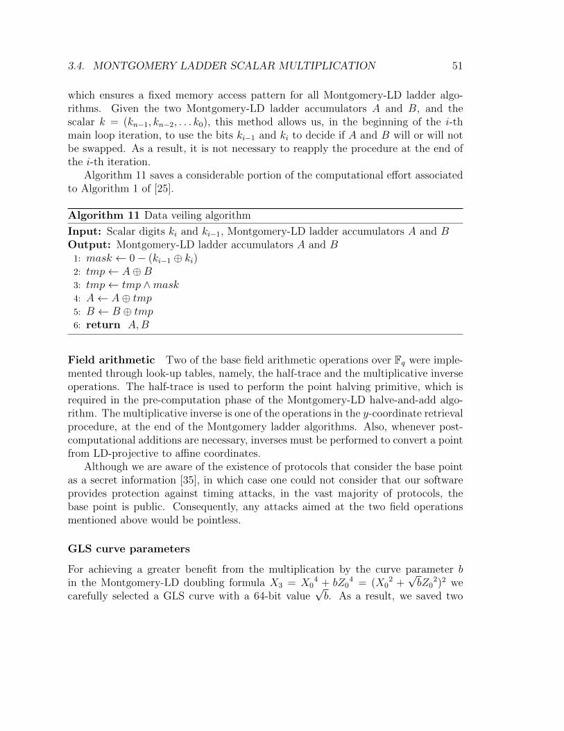
3.4. MONTGOMERY LADDER SCALAR MULTIPLICATION 51
which ensures a fixed memory access pattern for all Montgomery-LD ladder algo-rithms. Given the two Montgomery-LD ladder accumulators A and B, and thescalar k = (kn−1, kn−2, . . . k0), this method allows us, in the beginning of the i-thmain loop iteration, to use the bits ki−1 and ki to decide if A and B will or will notbe swapped. As a result, it is not necessary to reapply the procedure at the end ofthe i-th iteration.
Algorithm 11 saves a considerable portion of the computational effort associatedto Algorithm 1 of [25].
Algorithm 11 Data veiling algorithm
Input: Scalar digits ki and ki−1, Montgomery-LD ladder accumulators A and BOutput: Montgomery-LD ladder accumulators A and B
1: mask ← 0− (ki−1 ⊕ ki)2: tmp← A⊕B3: tmp← tmp ∧mask4: A← A⊕ tmp5: B ← B ⊕ tmp6: return A,B
Field arithmetic Two of the base field arithmetic operations over Fq were imple-mented through look-up tables, namely, the half-trace and the multiplicative inverseoperations. The half-trace is used to perform the point halving primitive, which isrequired in the pre-computation phase of the Montgomery-LD halve-and-add algo-rithm. The multiplicative inverse is one of the operations in the y-coordinate retrievalprocedure, at the end of the Montgomery ladder algorithms. Also, whenever post-computational additions are necessary, inverses must be performed to convert a pointfrom LD-projective to affine coordinates.
Although we are aware of the existence of protocols that consider the base pointas a secret information [35], in which case one could not consider that our softwareprovides protection against timing attacks, in the vast majority of protocols, thebase point is public. Consequently, any attacks aimed at the two field operationsmentioned above would be pointless.
GLS curve parameters
For achieving a greater benefit from the multiplication by the curve parameter bin the Montgomery-LD doubling formula X3 = X0
4 + bZ04 = (X0
2 +√bZ0
2)2 wecarefully selected a GLS curve with a 64-bit value
√b. As a result, we saved two
52 CHAPTER 3. GALBRAITH-LIN-SCOTT CURVES
carry-less multiplication and a dozen of SSE instructions per field multiplication.Next, we describe the parameters, as polynomials represented in hexadecimal, forour GLS curve Ea′,b/Fq2 : y2 + xy = x3 + a′x2 + b.
• a′ = u,
• b = 0x54045144410401544101540540515101,
•√b = 0xE2DA921E91E38DD1,
The 253-bit prime order r of the main subgroup of E/Fq2 is,
r =0x1FFFFFFFFFFFFFFFFFFFFFFFFFFFFFFFA6B89E49D3FECD828CA8D66BF4B88ED5.
Also, the integer δ such that ψ(P ) = δP for all P ∈ E(Fq2) is,
δ =0x74AEFB81EE8A42E9E9D0085E156A8EFBA3D302F9C74D737FA00360F9395C788.
The base point P = (x, y) of order r used in this work is,
x =0x4A21A3666CF9CAEBD812FA19DF9A3380 + 0x358D7917D6E9B5A7550B1B083BC299F3 · u,y =0x6690CB7B914B7C4018E7475D9C2B1C13 + 0x2AD4E15A695FD54011BA179D5F4B44FC · u.
Finally, the towering of our field Fq ∼= F2[x]/(f(x)) and its quadratic extensionFq2 ∼= Fq[u]/(g(x)) is constructed by means of the irreducible trinomials f(x) =x127 + x63 + 1 and g(u) = u2 + u+ 1.
Scalar multiplication timings
Our implementation was mainly designed for the Intel Haswell processor family,which supports vectorial sets such as SSE and AVX, a carry-less multiplication andsome bit manipulation instructions. The programming was done in C with the sup-port of assembly inline code. The compilation was performed via GCC version 4.7.3with the flags -m64 -march=core-avx2 -mtune=core-avx2 -O3 -funroll-loops
-fomit-frame-pointer. Finally, the timings were collected on an Intel Core i7-4700MQ, with the Turbo Boost and Hyperthreading features disabled.
Table 3.10 presents the experimental timings obtained for the most prominentbuilding blocks required for computing the point multiplication operation on theGLS binary elliptic curves.
We present, in Table 3.11, a comparison of our timings against a selection of state-of-the-art implementations of the point multiplication operation on binary and primeelliptic curves. Due to the Montgomery-LD point doubling efficiency, which costs
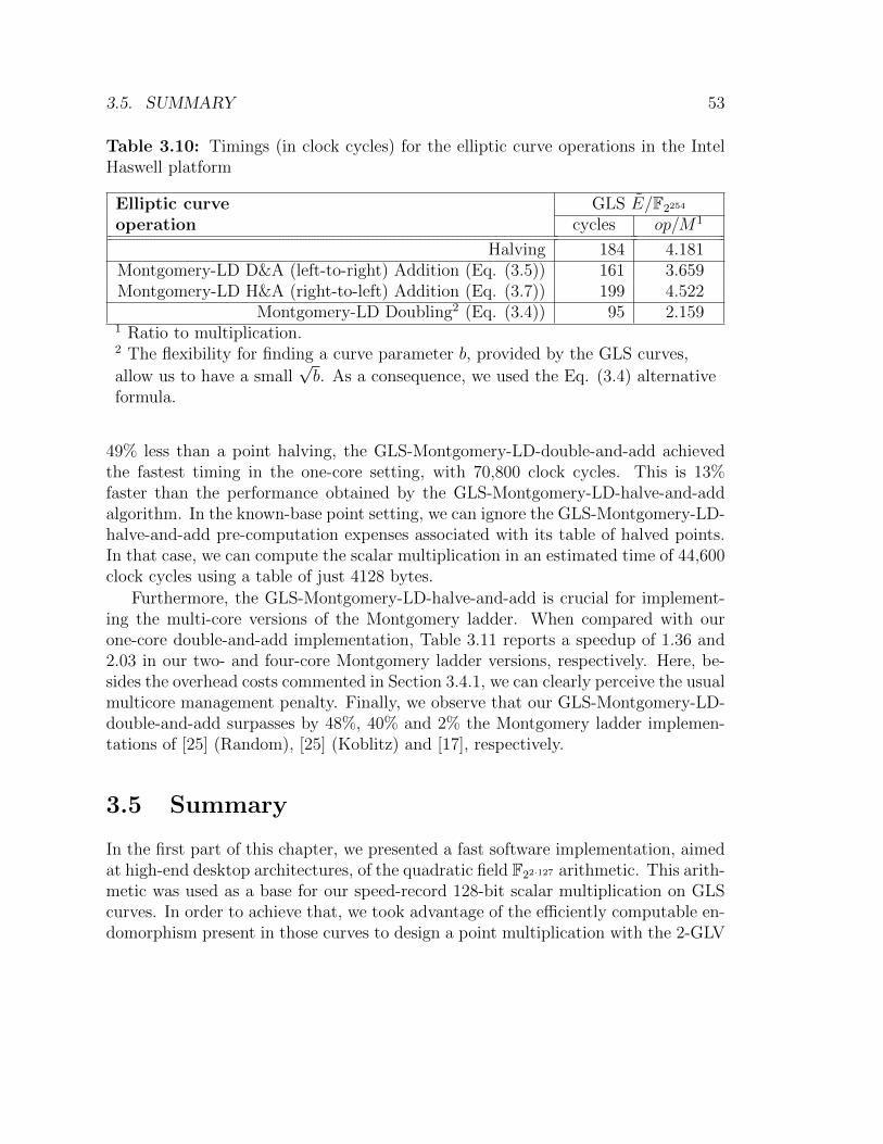
3.5. SUMMARY 53
Table 3.10: Timings (in clock cycles) for the elliptic curve operations in the IntelHaswell platform
Elliptic curveoperation
GLS E/F2254
cycles op/M1
Halving 184 4.181Montgomery-LD D&A (left-to-right) Addition (Eq. (3.5)) 161 3.659Montgomery-LD H&A (right-to-left) Addition (Eq. (3.7)) 199 4.522
Montgomery-LD Doubling2 (Eq. (3.4)) 95 2.1591 Ratio to multiplication.2 The flexibility for finding a curve parameter b, provided by the GLS curves,
allow us to have a small√b. As a consequence, we used the Eq. (3.4) alternative
formula.
49% less than a point halving, the GLS-Montgomery-LD-double-and-add achievedthe fastest timing in the one-core setting, with 70,800 clock cycles. This is 13%faster than the performance obtained by the GLS-Montgomery-LD-halve-and-addalgorithm. In the known-base point setting, we can ignore the GLS-Montgomery-LD-halve-and-add pre-computation expenses associated with its table of halved points.In that case, we can compute the scalar multiplication in an estimated time of 44,600clock cycles using a table of just 4128 bytes.
Furthermore, the GLS-Montgomery-LD-halve-and-add is crucial for implement-ing the multi-core versions of the Montgomery ladder. When compared with ourone-core double-and-add implementation, Table 3.11 reports a speedup of 1.36 and2.03 in our two- and four-core Montgomery ladder versions, respectively. Here, be-sides the overhead costs commented in Section 3.4.1, we can clearly perceive the usualmulticore management penalty. Finally, we observe that our GLS-Montgomery-LD-double-and-add surpasses by 48%, 40% and 2% the Montgomery ladder implemen-tations of [25] (Random), [25] (Koblitz) and [17], respectively.
3.5 Summary
In the first part of this chapter, we presented a fast software implementation, aimedat high-end desktop architectures, of the quadratic field F22·127 arithmetic. This arith-metic was used as a base for our speed-record 128-bit scalar multiplication on GLScurves. In order to achieve that, we took advantage of the efficiently computable en-domorphism present in those curves to design a point multiplication with the 2-GLV
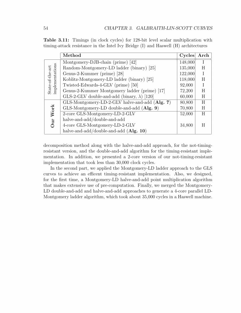
54 CHAPTER 3. GALBRAITH-LIN-SCOTT CURVES
Table 3.11: Timings (in clock cycles) for 128-bit level scalar multiplication withtiming-attack resistance in the Intel Ivy Bridge (I) and Haswell (H) architectures
Method Cycles Arch
Sta
te-o
f-th
e-ar
tim
ple
men
tati
ons Montgomery-DJB-chain (prime) [42] 148,000 I
Random-Montgomery-LD ladder (binary) [25] 135,000 HGenus-2-Kummer (prime) [28] 122,000 IKoblitz-Montgomery-LD ladder (binary) [25] 118,000 HTwisted-Edwards-4-GLV (prime) [50] 92,000 IGenus-2-Kummer Montgomery ladder (prime) [17] 72,200 HGLS-2-GLV double-and-add (binary, λ) [120] 60,000 H
Our
Work
GLS-Montgomery-LD-2-GLV halve-and-add (Alg. 7) 80,800 HGLS-Montgomery-LD double-and-add (Alg. 9) 70,800 H2-core GLS-Montgomery-LD-2-GLVhalve-and-add/double-and-add
52,000 H
4-core GLS-Montgomery-LD-2-GLVhalve-and-add/double-and-add (Alg. 10)
34,800 H
decomposition method along with the halve-and-add approach, for the not-timing-resistant version, and the double-and-add algorithm for the timing-resistant imple-mentation. In addition, we presented a 2-core version of our not-timing-resistantimplementation that took less than 30,000 clock cycles.
In the second part, we applied the Montgomery-LD ladder approach to the GLScurves to achieve an efficent timing-resistant implementation. Also, we designed,for the first time, a Montgomery-LD halve-and-add point multiplication algorithmthat makes extensive use of pre-computation. Finally, we merged the Montgomery-LD double-and-add and halve-and-add approaches to generate a 4-core parallel LD-Montgomery ladder algorithm, which took about 35,000 cycles in a Haswell machine.
4 | Koblitz Curves
The anomalous binary curves, generally referred to as Koblitz curves, are binaryelliptic curves which satisfies the following Weierstrass equation,
Ea : y2 + xy = x3 + ax2 + 1, (4.1)
with a ∈ {0, 1}. Since their introduction in 1991 by Neal Koblitz [99], these curveswere extensively studied for their additional structure that allows, in principle, aperformance speedup in the point multiplication computation.
Let q = 2m, with prime m. The set of affine points P = (x, y) ∈ Fq × Fq thatsatisfy Equation 4.1 together with a point at infinity represented as O, forms anabelian group denoted by Ea(F2m) of order #Ea(F2m) = 2 · (2− a) · r. Its group lawis defined by the point addition operation.
In λ-affine coordinates (see Chapter 2), where the points are represented asP = (x, λ = x+ y
x), x 6= 0, the λ-affine form of the curve equation becomes,
Ea : (λ2 + λ+ a)x2 = x4 + 1. (4.2)
The Frobenius map τ : Ea(Fq)→ Ea(Fq) defined by τ(O) = O, τ(x, y) = (x2, y2),is a curve automorphism satisfying (τ 2 + 2)P = µτ(P ) for µ = (−1)1−a and allP ∈ Ea(Fq). By solving the equation τ 2 + 2 = µτ , the Frobenius map can be seen asthe complex number τ = (µ±
√−7)/2. Notice that in λ-coordinates the Frobenius
map action remains the same. Let Λ be the function that tranforms the point coor-dinates from affine to λ-affine as Λ(x, y) = (x, x+ x
y), then τ(Λ(x, y)) = (x2, x2 + y2
x2),
which corresponds to the λ-representation of τ(x, y).Let Z[τ ] be the ring extension of Z. Since the Frobenius map is computationally
cheap, as long as it is possible to convert an integer scalar k to its τ -representationk =
∑l−1i=0 uiτ
i, with ui ∈ Z, its action can be exploited in a point multiplication com-putation by adding multiples uiτ
i(P ). Solinas [145] proposed exactly that, namely, aτ -adic scalar recoding analogous to the signed digit scalar non-adjacent form (NAF)representation.
55
56 CHAPTER 4. KOBLITZ CURVES
From the security point of view, it has been argued that the availability of ad-ditional structure in the form of endomorphisms can be a potential threat to thehardness of elliptic curve discrete logarithms [20], but limitations observed in ap-proaches based on isogeny walks is evidence to the contrary [97]. Furthermore, thegeneration of Koblitz curves satisfy by definition the rigidity property in the moststrict sense1.
Constant-time compact implementations for Koblitz curves are also easily ob-tained by specializing the Montgomery-Lopez-Dahab ladder algorithm [104] for thecurve parameter b = 1, although we show below that this is not the most efficientconstant-time implementation strategy possible. Another practical advantage is theadoption of Koblitz curves by several standards bodies [131], which guarantee in-teroperability and availability of implementations in many hardware and softwareplatforms.
The present chapter is divided into two parts. First, a regular τ -adic recodingmethod, which is a necessary step in order to implement a timing-resistant scalarmultiplication on Koblitz curves, is proposed. Second, the new recoding method isused to introduce a 128-bit secure protected point multiplication on a new family ofKoblitz curves defined over F4.
4.1 A novel regular τ-adic approach
Let r be a prime order of a subgroup of Ea(Fq) and k a scalar in Zr. The recodingapproach proposed by Solinas [145] finds an element ρ ∈ Z[τ ], of minimal norm aspossible, such that ρ ≡ k (mod τm−1
τ−1). A τ -adic expansion with average non-zero
density 13
can be obtained by repeatedly dividing ρ by τ and assigning the remainders
to the digits ui to obtain k =∑i=l−1
i=0 uiτi. An alternative approach that does not
involve multi-precision divisions, is to compute the partial reduction2 of the elementk as ρ = k partmod
(τm−1τ−1
).
A width-w τ -NAF expansion with non-zero density 1w+1
, where at most one of anyw consecutive coefficients is non-zero, can also be obtained by repeatedly dividingρ′ by τw and assigning the remainders to the digit set {0,±α1,±α3, . . . ,±α2w−1−1},for αi = i mod τw. Under reasonable assumptions, this window-based recoding haslength l ≤ m+ 1 [145].
1The only degree of freedom in the curve generation process consists in choosing a suitable primedegree extension m that produces a curve with almost-prime order.
2The operation is denoted as partmod in [145].
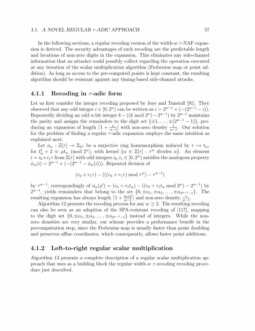
4.1. A NOVEL REGULAR τ -ADIC APPROACH 57
In the following sections, a regular recoding version of the width-w τ -NAF expan-sion is derived. The security advantages of such recoding are the predictable lengthand locations of non-zero digits in the expansion. This eliminates any side-channelinformation that an attacker could possibly collect regarding the operation executedat any iteration of the scalar multiplication algorithm (Frobenius map or point ad-dition). As long as access to the pre-computed points is kept constant, the resultingalgorithm should be resistant against any timing-based side-channel attacks.
4.1.1 Recoding in τ-adic form
Let us first consider the integer recoding proposed by Joye and Tunstall [91]. Theyobserved that any odd integer i ∈ [0, 2w) can be written as i = 2w−1 + (−(2w−1 − i)).Repeatedly dividing an odd n-bit integer k− ((k mod 2w)−2w−1) by 2w−1 maintainsthe parity and assigns the remainders to the digit set {±1, . . . ,±(2w−1 − 1)}, pro-ducing an expansion of length d1 + n
w−1] with non-zero density 1
w−1. Our solution
for the problem of finding a regular τ -adic expansion employs the same intuition asexplained next.
Let φw : Z[τ ] → Z2w be a surjective ring homomorphism induced by τ 7→ tw,for t2w + 2 ≡ µtw (mod 2w), with kernel {α ∈ Z[τ ] : τw divides α}. An elementi = i0+i1τ from Z[τ ] with odd integers i0, i1 ∈ [0, 2w) satisfies the analogous propertyφw(i) = 2w−1 + (−(2w−1 − φw(i))). Repeated division of
(r0 + r1τ)− (((r0 + r1τ) mod τw)− τw−1)
by τw−1, correspondingly of φw(ρ′) = (r0 + r1tw) − ((r0 + r1tw mod 2w) − 2w−1) by2w−1, yields remainders that belong to the set {0,±α1,±α3, . . . ,±α2w−1−1}. Theresulting expansion has always length d1 + m+2
w−1e and non-zero density 1
w−1.
Algorithm 12 presents the recoding process for any w ≥ 2. The resulting recodingcan also be seen as an adaption of the SPA-resistant recoding of [117], mappingto the digit set {0,±α1,±α3, . . . ,±α2w−1−1} instead of integers. While the non-zero densities are very similar, our scheme provides a performance benefit in theprecomputation step, since the Frobenius map is usually faster than point doublingand preserves affine coordinates, which consequently, allows faster point additions.
4.1.2 Left-to-right regular scalar multiplication
Algorithm 13 presents a complete description of a regular scalar multiplication ap-proach that uses as a building block the regular width-w τ -recoding recoding proce-dure just described.
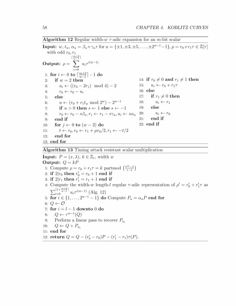
58 CHAPTER 4. KOBLITZ CURVES
Algorithm 12 Regular width-w τ -adic expansion for an m-bit scalar
Input: w, tw, αu = βu+γuτ for u = {±1,±3,±5, . . . ,±2w−1−1}, ρ = r0+r1τ ∈ Z[τ ]with odd r0, r1
Output: ρ =
dm+2w−1e∑
i=0
uiτi(w−1)
1: for i← 0 to dm+2w−1e - 1 do
2: if w = 2 then3: ui ← ((r0 − 2r1) mod 4)− 24: r0 ← r0 − ui5: else6: u← (r0 + r1tw mod 2w)− 2w−1
7: if u > 0 then s← 1 else s← −18: r0 ← r0 − sβu, r1 ← r1 − sγu, ui ← sαu9: end if
10: for j ← 0 to (w − 2) do11: t← r0, r0 ← r1 + µr0/2, r1 ← −t/212: end for13: end for
14: if r0 6= 0 and r1 6= 1 then15: ui ← r0 + r1τ16: else17: if r1 6= 0 then18: ui ← r1
19: else20: ui ← r0
21: end if22: end if
Algorithm 13 Timing attack resistant scalar multiplication
Input: P = (x, λ), k ∈ Zr, width wOutput: Q = kP
1: Compute ρ = r0 + r1τ = k partmod(τm−1τ−1
)2: if 2|r0 then r′0 = r0 + 1 end if3: if 2|r1 then r′1 = r1 + 1 end if4: Compute the width-w length-l regular τ -adic representation of ρ′ = r′0 + r′1τ as∑d1+m+2
w−1e
i=0 uiτi(w−1) (Alg. 12)
5: for i ∈ {1, . . . , 2w−1 − 1} do Compute Pu = αuP end for6: Q← O7: for i = l − 1 downto 0 do8: Q← τw−1(Q)9: Perform a linear pass to recover Pui
10: Q← Q+ Pui11: end for12: return Q = Q− (r′0 − r0)P − (r′1 − r1)τ(P ).
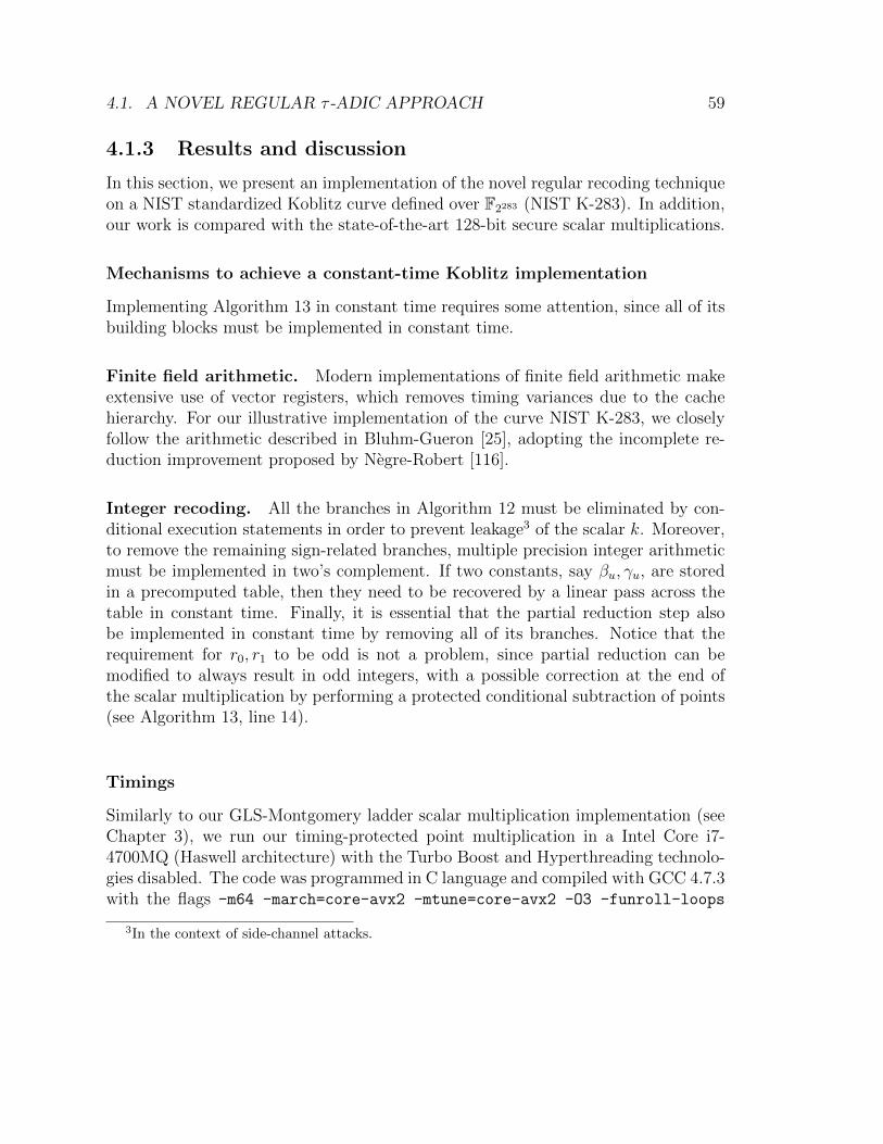
4.1. A NOVEL REGULAR τ -ADIC APPROACH 59
4.1.3 Results and discussion
In this section, we present an implementation of the novel regular recoding techniqueon a NIST standardized Koblitz curve defined over F2283 (NIST K-283). In addition,our work is compared with the state-of-the-art 128-bit secure scalar multiplications.
Mechanisms to achieve a constant-time Koblitz implementation
Implementing Algorithm 13 in constant time requires some attention, since all of itsbuilding blocks must be implemented in constant time.
Finite field arithmetic. Modern implementations of finite field arithmetic makeextensive use of vector registers, which removes timing variances due to the cachehierarchy. For our illustrative implementation of the curve NIST K-283, we closelyfollow the arithmetic described in Bluhm-Gueron [25], adopting the incomplete re-duction improvement proposed by Negre-Robert [116].
Integer recoding. All the branches in Algorithm 12 must be eliminated by con-ditional execution statements in order to prevent leakage3 of the scalar k. Moreover,to remove the remaining sign-related branches, multiple precision integer arithmeticmust be implemented in two’s complement. If two constants, say βu, γu, are storedin a precomputed table, then they need to be recovered by a linear pass across thetable in constant time. Finally, it is essential that the partial reduction step alsobe implemented in constant time by removing all of its branches. Notice that therequirement for r0, r1 to be odd is not a problem, since partial reduction can bemodified to always result in odd integers, with a possible correction at the end ofthe scalar multiplication by performing a protected conditional subtraction of points(see Algorithm 13, line 14).
Timings
Similarly to our GLS-Montgomery ladder scalar multiplication implementation (seeChapter 3), we run our timing-protected point multiplication in a Intel Core i7-4700MQ (Haswell architecture) with the Turbo Boost and Hyperthreading technolo-gies disabled. The code was programmed in C language and compiled with GCC 4.7.3with the flags -m64 -march=core-avx2 -mtune=core-avx2 -O3 -funroll-loops
3In the context of side-channel attacks.

60 CHAPTER 4. KOBLITZ CURVES
-fomit-frame-pointer. In Table 4.1 we present the costs of the functions thatform the base of our protected NIST K-283 point multiplication.
Table 4.1: Timings (in clock cycles) for the NIST K-283 elliptic curve operations
Elliptic curveoperation
Koblitz E/F2283
cycles op/m1
Frobenius 70 1.235Integer τ -adic recoding (Alg. 12) (w = 5) 8,900 156.863
Point addition 602 10.5881 Ratio to multiplication in F2283 .
In Table 4.2, we show our scalar multiplication results. For benchmarking pur-poses we also included a baseline implementation of the customary MontgomeryLopez-Dahab ladder. This allows easier comparisons with related work and permitsto evaluate the impact of incomplete reduction in the field arithmetic performance.
Table 4.2: Timings (in clock cycles) for different 128-bit secure scalar multiplicationimplementations with timing-attack resistance in the Intel Ivy Bridge (I) and Haswell(H) architectures
Method Cycles Arch
Sta
te-of-th
e-art
implementa
tions Montgomery-DJB-chain (prime) [42] 148,000 I
Random-Montgomery-LD ladder (binary) [25] 135,000 HGenus-2-Kummer (prime) [28] 122,000 IKoblitz-Montgomery-LD ladder (binary) [25] 118,000 HTwisted-Edwards-4-GLV (prime) [50] 92,000 IGenus-2-Kummer Montgomery ladder (prime) [17] 72,200 HGLS-2-GLV double-and-add (binary, λ) [120] 60,000 H
Our WorkKoblitz-Montgomery-LD (left-to-right) 122,000 HKoblitz-regular τ -and-add (left-to-right, w = 5) 99,000 H
The fast τ endomorphism allows us to have a regular-recoding implementationthat outperforms a standard Montgomery ladder for Koblitz curves by 18%. Inaddition, our fastest Koblitz code surpasses by 16% the recent implementation re-ported in [25] 4. Finally, note that, in spite of the fact that the τ endomorphism is
4We could not reproduce the timing of 118,000 cycles with the code available from [25], whichindicates that TurboBoost could be possibly turned on on their benchmarks. Considering this,

4.2. KOBLITZ CURVES OVER F4 61
26% faster than the Montgomery-LD point doubling, the superior efficiency of theGLS quadratic field arithmetic produces faster results for the GLS double-and-addalgorithm.
4.2 Koblitz curves over F4
Koblitz curves defined over F4 were also proposed in 1991 by Neal Koblitz [99].However, until nowadays, works related to Koblitz curves have analyzed the securityand performance of curves defined only over F2m , with prime m (for instance, [148,9, 155]). On the other hand, it has been shown recently [120, 103] that the quadraticextension field arithmetic is quite efficient when implemented in software. This isbecause we execute the same operation in each base element of the extension fieldelement. For instance, given the quadratic field elements a = a0+a1i and b = b0+b1i,the addition c = a+b can be performed as c = (a0+b0)+(a1+b1)i (for more examples,see Section 3.1.6). As a result, we can fully employ the current high-end processorspipelines and their inherent instruction-level parallelism.
In this work, we designed and implemented, for the first time, a 128-bit secureand timing attack resistant scalar multiplication on a Koblitz curve defined overF4. In the next sections, we present the details of the Koblitz curves defined overquadratic extensions along with the field arithmetic functions. Finally, we discussour implementation timings and compare it against the state-of-the-art works.
4.2.1 Introduction
Let q = 2m, with prime m. Koblitz curves over F4 are defined by the followingequation
Ea : y2 + xy = x3 + aγx2 + γ, (4.3)
where γ ∈ F22 satisfies γ2 = γ + 1 and a ∈ {0, 1}.It is known that, for each proper divisor l of k, E(F4l) is a subgroup of E(F4k)
and #E(F4l) divides #E(F4k). Since m is prime, Ea(F4m) can have almost-primeorder (for instance, E0(F22·163) and E1(F22·167)).
Note that #E0(F4) = 4 and #E1(F4) = 6. In Table 4.3, we present the grouporders #Ea(F4m) of Koblitz curves defined over F4 for prime degrees m ∈ [127, 191].
our implementation of Koblitz-Montgomery-LD becomes 9% faster than [25], reflecting the savingsfrom partial reduction, and the speedup achieved by the Koblitz-regular implementation increasesto 26%.
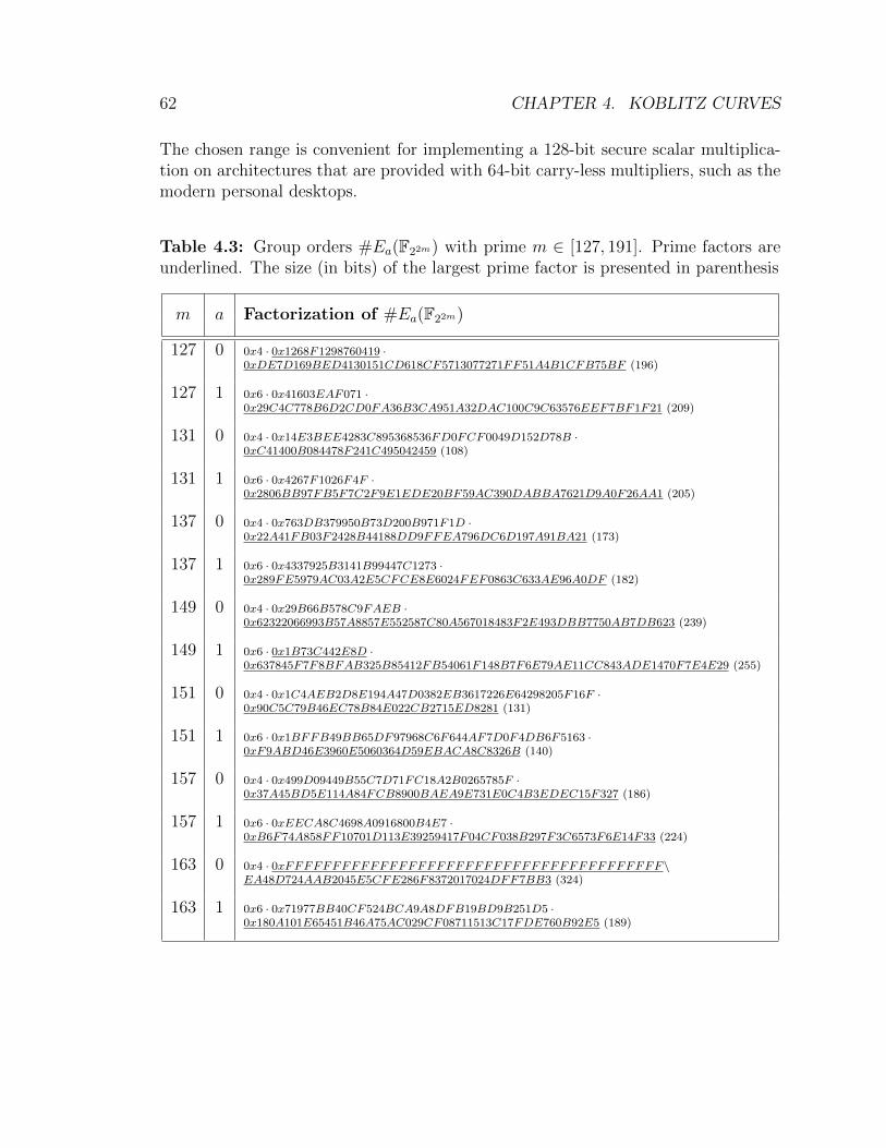
62 CHAPTER 4. KOBLITZ CURVES
The chosen range is convenient for implementing a 128-bit secure scalar multiplica-tion on architectures that are provided with 64-bit carry-less multipliers, such as themodern personal desktops.
Table 4.3: Group orders #Ea(F22m) with prime m ∈ [127, 191]. Prime factors areunderlined. The size (in bits) of the largest prime factor is presented in parenthesis
m a Factorization of #Ea(F22m)
127 0 0x4 · 0x1268F1298760419 ·0xDE7D169BED4130151CD618CF5713077271FF51A4B1CFB75BF (196)
127 1 0x6 · 0x41603EAF071 ·0x29C4C778B6D2CD0FA36B3CA951A32DAC100C9C63576EEF7BF1F21 (209)
131 0 0x4 · 0x14E3BEE4283C895368536FD0FCF0049D152D78B ·0xC41400B084478F241C495042459 (108)
131 1 0x6 · 0x4267F1026F4F ·0x2806BB97FB5F7C2F9E1EDE20BF59AC390DABBA7621D9A0F26AA1 (205)
137 0 0x4 · 0x763DB379950B73D200B971F1D ·0x22A41FB03F2428B44188DD9FFEA796DC6D197A91BA21 (173)
137 1 0x6 · 0x4337925B3141B99447C1273 ·0x289FE5979AC03A2E5CFCE8E6024FEF0863C633AE96A0DF (182)
149 0 0x4 · 0x29B66B578C9FAEB ·0x62322066993B57A8857E552587C80A567018483F2E493DBB7750AB7DB623 (239)
149 1 0x6 · 0x1B73C442E8D ·0x637845F7F8BFAB325B85412FB54061F148B7F6E79AE11CC843ADE1470F7E4E29 (255)
151 0 0x4 · 0x1C4AEB2D8E194A47D0382EB3617226E64298205F16F ·0x90C5C79B46EC78B84E022CB2715ED8281 (131)
151 1 0x6 · 0x1BFFB49BB65DF97968C6F644AF7D0F4DB6F5163 ·0xF9ABD46E3960E5060364D59EBACA8C8326B (140)
157 0 0x4 · 0x499D09449B55C7D71FC18A2B0265785F ·0x37A45BD5E114A84FCB8900BAEA9E731E0C4B3EDEC15F327 (186)
157 1 0x6 · 0xEECA8C4698A0916800B4E7 ·0xB6F74A858FF10701D113E39259417F04CF038B297F3C6573F6E14F33 (224)
163 0 0x4 · 0xFFFFFFFFFFFFFFFFFFFFFFFFFFFFFFFFFFFFFFFF\EA48D724AAB2045E5CFE286F8372017024DFF7BB3 (324)
163 1 0x6 · 0x71977BB40CF524BCA9A8DFB19BD9B251D5 ·0x180A101E65451B46A75AC029CF08711513C17FDE760B92E5 (189)
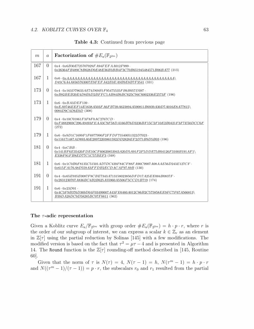
4.2. KOBLITZ CURVES OVER F4 63
Table 4.3: Continued from previous page
m a Factorization of #Ea(F22m)
167 0 0x4 · 0x6B30E725707929FA94FEFAA012F999 ·0x26364FB489C8B628D0E48E36B3BB4F3C70B651945484571B06BA77 (213)
167 1 0x6 · 0xAAAAAAAAAAAAAAAAAAAAAAAAAAAAAAAAAAAAAAAAA\D45C6A4A8565763007E9FEFA42E0EA9B9E8B7F3541 (331)
173 0 0x4 · 0x163D79633AE74D69B1F95475535FB6B057D397 ·0xB82BEB20E4D8E6D2BFFC1AB84B6BC625C94C6002336E2573F (196)
173 1 0x6 · 0xBA3DEF139 ·0xEA9746EEF14E1638A503FA6FB739A623894A590811B6939A30D7A016E8A77815\0084D9C4D6E0D (308)
179 0 0x4 · 0x10C01861F3F8F0AC2767CD ·0xF4882969C296A9493FEAA3C9F58DA166B76D3236BF15C2F10E2B0421F3F7E50DCC6F(272)
179 1 0x6 · 0x9D1C1699F1F6977990F2FFDF75540051322D7023 ·0x116171487AD893A0E28972203861592DD2828EF2D71B9D5B03 (196)
181 0 0x4 · 0xCBB ·0x141BF6E35420FDE10CF60620853943A20D5A91F2F5DDE75B04126F3100B191AF1\E338F81FB8ED77C1C57BEF3 (348)
181 1 0x6 · 0x1C0B0F8135C51501AD7DC439F84CF88FA90C9907A08AAE56D243E127CF ·0x615FA176A8D559A3FFDB2ECDACAF97A9B (130)
191 0 0x4 · 0x65E935E0087F8CBE7343A713158023856DFD17A25EE004B0837F ·0x2831230707A836BC4B2B625A55960A5506F5CCD1B719 (174)
191 1 0x6 · 0x23D01 ·0x4C3F9B376D369D04F03499007A43FE6460A012C86B2C575858EE9FC7F67A566813\B39DA28DC9D58285BC07F8811 (362)
The τ-adic representation
Given a Koblitz curve Ea/F22m with group order #Ea(F22m) = h · p · r, where r isthe order of our subgroup of interest, we can express a scalar k ∈ Zr as an elementin Z[τ ] using the partial reduction by Solinas [145] with a few modifications. Themodified version is based on the fact that τ 2 = µτ − 4 and is presented in Algorithm14. The Round function is the Z[τ ] rounding-off method described in [145, Routine60].
Given that the norm of τ is N(τ) = 4, N(τ − 1) = h, N(τm − 1) = h · p · rand N((τm − 1)/(τ − 1)) = p · r, the subscalars r0 and r1 resulted from the partial

64 CHAPTER 4. KOBLITZ CURVES
Algorithm 14 Partial reduction modulo (τm − 1)/(τ − 1)
Input: The scalar k ∈ [1, r − 1], s0 = d0 + µd1, s1 = −d1, where(τm − 1)/(τ − 1) = d0 + d1τ
Output: ρ = (r0 + r1τ) = k partmod (τm − 1)/(τ − 1)1: t← s0 + µ · s1
2: λ0 ← s0 · k/(p · r)3: λ1 ← s1 · k/(p · r)4: q0, q1 ← Round(λ0, λ1)5: r0 ← k − t · q0 − 4 · s1 · q1
6: r1 ← s1 · q0 − s0 · q1
7: return (r0, r1).
modulo function will be both of size approximately (p · r)/2. As a consequence, ourscalar multiplication will need more iterations than expected, since it will considerthe order p of a subgroup which is not of cryptographic interest.
For that reason, we considered that the input scalar of our point multiplicationalgorithm is already represented in Z[τ ]. As a result, it is not required to perform apartial reduction in the scalar k, and the number of iterations in the point multipli-cation will be consistent with the scalar k size. If one needs to retrieve the scalar krepresented in Zr, it can be easily computed with one multiplication and one additionin Zr. This design decision was based on the degree-2 scalar decomposition method,in the GLS curves context, suggested in [61].
The width-w τNAF form
After representing the scalar k in Z[τ ], we can apply the slightly modified version ofthe Algorithm 12 in order to express the scalar in the regular width-w τNAF form.The adjusted method is presented in Algorithm 15.
Given a width w, after running Algorithm 15, we have 22(w−1)−1 digits5. As aresult, it is necessary to be more conservative when choosing the width w, whencompared to the Koblitz curves defined over F2. For widths w = 2, 3, 4, 5 we haveto pre- or post-compute 2, 8, 32 and 128 points, respectively. For the 128-bit pointmultiplication, we estimated that the value of the width w must be at most four,otherwise, the costs of the point pre/post-processing are greater than the additionsavings obtained in the main iteration.
5We are considering only positive digits, since the cost of applying signs to points in binaryelliptic curves is negligible.
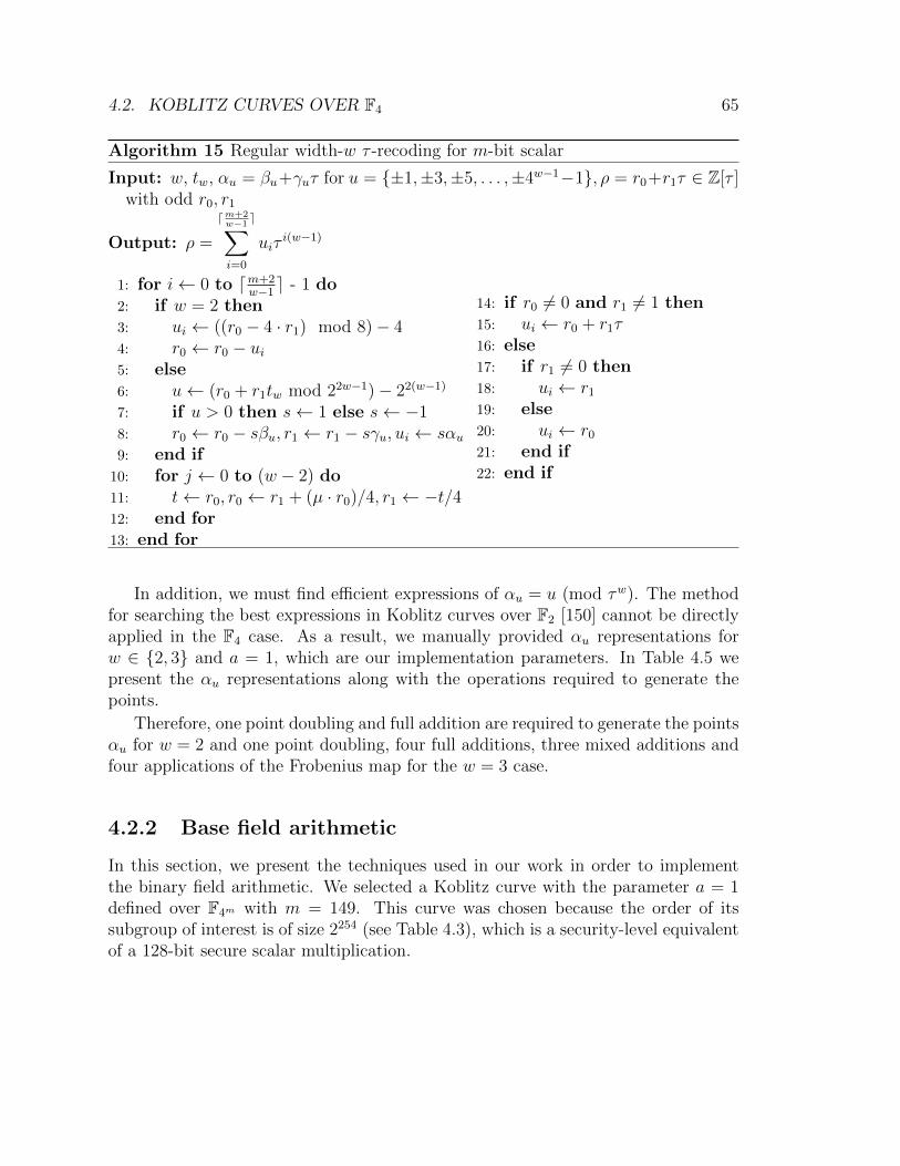
4.2. KOBLITZ CURVES OVER F4 65
Algorithm 15 Regular width-w τ -recoding for m-bit scalar
Input: w, tw, αu = βu+γuτ for u = {±1,±3,±5, . . . ,±4w−1−1}, ρ = r0+r1τ ∈ Z[τ ]with odd r0, r1
Output: ρ =
dm+2w−1e∑
i=0
uiτi(w−1)
1: for i← 0 to dm+2w−1e - 1 do
2: if w = 2 then3: ui ← ((r0 − 4 · r1) mod 8)− 44: r0 ← r0 − ui5: else6: u← (r0 + r1tw mod 22w−1)− 22(w−1)
7: if u > 0 then s← 1 else s← −18: r0 ← r0 − sβu, r1 ← r1 − sγu, ui ← sαu9: end if
10: for j ← 0 to (w − 2) do11: t← r0, r0 ← r1 + (µ · r0)/4, r1 ← −t/412: end for13: end for
14: if r0 6= 0 and r1 6= 1 then15: ui ← r0 + r1τ16: else17: if r1 6= 0 then18: ui ← r1
19: else20: ui ← r0
21: end if22: end if
In addition, we must find efficient expressions of αu = u (mod τw). The methodfor searching the best expressions in Koblitz curves over F2 [150] cannot be directlyapplied in the F4 case. As a result, we manually provided αu representations forw ∈ {2, 3} and a = 1, which are our implementation parameters. In Table 4.5 wepresent the αu representations along with the operations required to generate thepoints.
Therefore, one point doubling and full addition are required to generate the pointsαu for w = 2 and one point doubling, four full additions, three mixed additions andfour applications of the Frobenius map for the w = 3 case.
4.2.2 Base field arithmetic
In this section, we present the techniques used in our work in order to implementthe binary field arithmetic. We selected a Koblitz curve with the parameter a = 1defined over F4m with m = 149. This curve was chosen because the order of itssubgroup of interest is of size 2254 (see Table 4.3), which is a security-level equivalentof a 128-bit secure scalar multiplication.
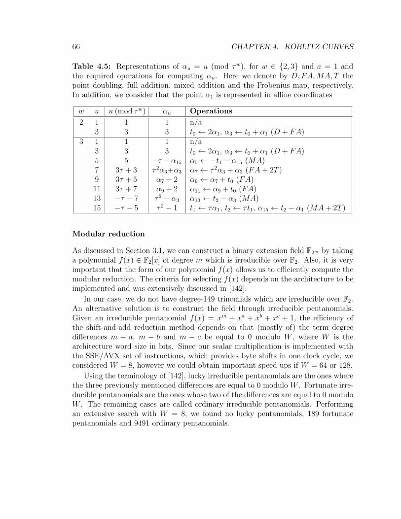
66 CHAPTER 4. KOBLITZ CURVES
Table 4.5: Representations of αu = u (mod τw), for w ∈ {2, 3} and a = 1 andthe required operations for computing αu. Here we denote by D,FA,MA, T thepoint doubling, full addition, mixed addition and the Frobenius map, respectively.In addition, we consider that the point α1 is represented in affine coordinates
w u u (mod τw) αu Operations
2 1 1 1 n/a3 3 3 t0 ← 2α1, α3 ← t0 + α1 (D + FA)
3 1 1 1 n/a3 3 3 t0 ← 2α1, α3 ← t0 + α1 (D + FA)5 5 −τ −α15 α5 ← −t1 − α15 (MA)7 3τ + 3 τ 2α3+α3 α7 ← τ 2α3 + α3 (FA+ 2T )9 3τ + 5 α7 + 2 α9 ← α7 + t0 (FA)11 3τ + 7 α9 + 2 α11 ← α9 + t0 (FA)13 −τ − 7 τ 2 − α3 α13 ← t2 − α3 (MA)15 −τ − 5 τ 2 − 1 t1 ← τα1, t2 ← τt1, α15 ← t2 − α1 (MA+ 2T )
Modular reduction
As discussed in Section 3.1, we can construct a binary extension field F2m by takinga polynomial f(x) ∈ F2[x] of degree m which is irreducible over F2. Also, it is veryimportant that the form of our polynomial f(x) allows us to efficiently compute themodular reduction. The criteria for selecting f(x) depends on the architecture to beimplemented and was extensively discussed in [142].
In our case, we do not have degree-149 trinomials which are irreducible over F2.An alternative solution is to construct the field through irreducible pentanomials.Given an irreducible pentanomial f(x) = xm + xa + xb + xc + 1, the efficiency ofthe shift-and-add reduction method depends on that (mostly of) the term degreedifferences m − a, m − b and m − c be equal to 0 modulo W , where W is thearchitecture word size in bits. Since our scalar multiplication is implemented withthe SSE/AVX set of instructions, which provides byte shifts in one clock cycle, weconsidered W = 8, however we could obtain important speed-ups if W = 64 or 128.
Using the terminology of [142], lucky irreducible pentanomials are the ones wherethe three previously mentioned differences are equal to 0 modulo W . Fortunate irre-ducible pentanomials are the ones whose two of the differences are equal to 0 moduloW . The remaining cases are called ordinary irreducible pentanomials. Performingan extensive search with W = 8, we found no lucky pentanomials, 189 fortunatepentanomials and 9491 ordinary pentanomials.
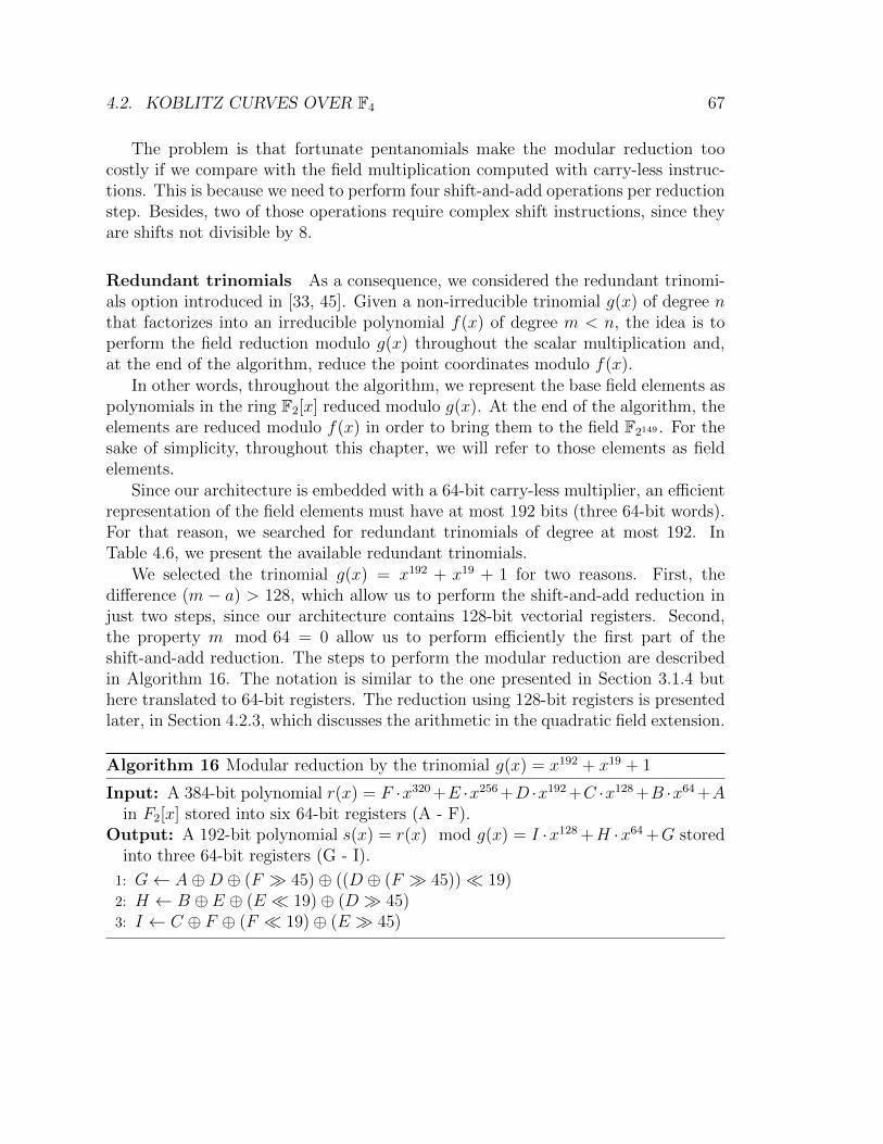
4.2. KOBLITZ CURVES OVER F4 67
The problem is that fortunate pentanomials make the modular reduction toocostly if we compare with the field multiplication computed with carry-less instruc-tions. This is because we need to perform four shift-and-add operations per reductionstep. Besides, two of those operations require complex shift instructions, since theyare shifts not divisible by 8.
Redundant trinomials As a consequence, we considered the redundant trinomi-als option introduced in [33, 45]. Given a non-irreducible trinomial g(x) of degree nthat factorizes into an irreducible polynomial f(x) of degree m < n, the idea is toperform the field reduction modulo g(x) throughout the scalar multiplication and,at the end of the algorithm, reduce the point coordinates modulo f(x).
In other words, throughout the algorithm, we represent the base field elements aspolynomials in the ring F2[x] reduced modulo g(x). At the end of the algorithm, theelements are reduced modulo f(x) in order to bring them to the field F2149 . For thesake of simplicity, throughout this chapter, we will refer to those elements as fieldelements.
Since our architecture is embedded with a 64-bit carry-less multiplier, an efficientrepresentation of the field elements must have at most 192 bits (three 64-bit words).For that reason, we searched for redundant trinomials of degree at most 192. InTable 4.6, we present the available redundant trinomials.
We selected the trinomial g(x) = x192 + x19 + 1 for two reasons. First, thedifference (m − a) > 128, which allow us to perform the shift-and-add reduction injust two steps, since our architecture contains 128-bit vectorial registers. Second,the property m mod 64 = 0 allow us to perform efficiently the first part of theshift-and-add reduction. The steps to perform the modular reduction are describedin Algorithm 16. The notation is similar to the one presented in Section 3.1.4 buthere translated to 64-bit registers. The reduction using 128-bit registers is presentedlater, in Section 4.2.3, which discusses the arithmetic in the quadratic field extension.
Algorithm 16 Modular reduction by the trinomial g(x) = x192 + x19 + 1
Input: A 384-bit polynomial r(x) = F ·x320 +E ·x256 +D ·x192 +C ·x128 +B ·x64 +Ain F2[x] stored into six 64-bit registers (A - F).
Output: A 192-bit polynomial s(x) = r(x) mod g(x) = I ·x128 +H ·x64 +G storedinto three 64-bit registers (G - I).
1: G← A⊕D ⊕ (F � 45)⊕ ((D ⊕ (F � 45))� 19)2: H ← B ⊕ E ⊕ (E � 19)⊕ (D � 45)3: I ← C ⊕ F ⊕ (F � 19)⊕ (E � 45)
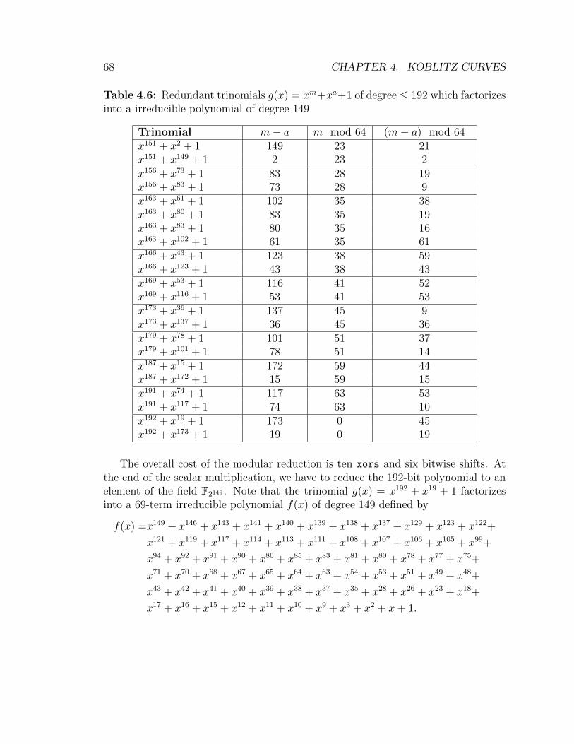
68 CHAPTER 4. KOBLITZ CURVES
Table 4.6: Redundant trinomials g(x) = xm+xa+1 of degree ≤ 192 which factorizesinto a irreducible polynomial of degree 149
Trinomial m− a m mod 64 (m− a) mod 64x151 + x2 + 1 149 23 21x151 + x149 + 1 2 23 2x156 + x73 + 1 83 28 19x156 + x83 + 1 73 28 9x163 + x61 + 1 102 35 38x163 + x80 + 1 83 35 19x163 + x83 + 1 80 35 16x163 + x102 + 1 61 35 61x166 + x43 + 1 123 38 59x166 + x123 + 1 43 38 43x169 + x53 + 1 116 41 52x169 + x116 + 1 53 41 53x173 + x36 + 1 137 45 9x173 + x137 + 1 36 45 36x179 + x78 + 1 101 51 37x179 + x101 + 1 78 51 14x187 + x15 + 1 172 59 44x187 + x172 + 1 15 59 15x191 + x74 + 1 117 63 53x191 + x117 + 1 74 63 10x192 + x19 + 1 173 0 45x192 + x173 + 1 19 0 19
The overall cost of the modular reduction is ten xors and six bitwise shifts. Atthe end of the scalar multiplication, we have to reduce the 192-bit polynomial to anelement of the field F2149 . Note that the trinomial g(x) = x192 + x19 + 1 factorizesinto a 69-term irreducible polynomial f(x) of degree 149 defined by
f(x) =x149 + x146 + x143 + x141 + x140 + x139 + x138 + x137 + x129 + x123 + x122+
x121 + x119 + x117 + x114 + x113 + x111 + x108 + x107 + x106 + x105 + x99+
x94 + x92 + x91 + x90 + x86 + x85 + x83 + x81 + x80 + x78 + x77 + x75+
x71 + x70 + x68 + x67 + x65 + x64 + x63 + x54 + x53 + x51 + x49 + x48+
x43 + x42 + x41 + x40 + x39 + x38 + x37 + x35 + x28 + x26 + x23 + x18+
x17 + x16 + x15 + x12 + x11 + x10 + x9 + x3 + x2 + x+ 1.

4.2. KOBLITZ CURVES OVER F4 69
The final reduction is performed via the mul-and-add reduction6 which, exper-imentally, performed more efficiently than the shift-and-add reduction. Concisely,the mul-and-add technique consists in a series of steps which includes shifts (in orderto align the bits in the registers), carry-less multiplications and xors for eliminatingthe extra bits.
The basic mul-and-add step is described in Algorithm 17. Here, besides the usualnotation, we represent the 64-bit carry-less multiplication by the symbol ×ij, wherei, j = {L,H}, with L and H representing the lowest and highest 64-bit word packedin a 128-bit register, respectively. For example, if we want to multiply the 128-bitregister A lowest 64-bit word by the 128-bit register B highest 64-bit word, we wouldexpress this operation as T ← A×LH B.
Algorithm 17 Basic step of the mul-and-add reduction modulo the 69-term irre-ducible polynomial f(x)
Input: A j-bit polynomial r(x) = B · x128 + A stored into two 128-bit registers(A, B), the irreducible polynomial f(x) = F · x128 + E stored into two 128-bitregisters (E, F).
Output: A (j−3)-bit polynomial s(x) = D·x128+C stored into two 128-bit registers(C, D).
1: T0 ← B � 21 (64-bit word alignment, 149 mod 64 = 21)2: T1 ← E ×LL T0
3: T2 ← E ×HL T0
4: T0 ← F ×LL T0
5: T1 ← T1 ⊕ (T2 � 64)6: T0 ← T0 ⊕ (T2 � 64)7: C ← A⊕ T1
8: D ← B ⊕ T0
The algorithm requires four xors, three bitwise shifts and three carry-less multi-plications. In our particular case, the difference between the degrees of the two mostsignificant monomials of f(x) is three. Also, note that we need to reduce 43 bits(191-148). As a result, it is required d43
3e = 15 applications of the Algorithm 17 in
order to conclude the reduction.
6For a more detailed explanation of the shift-and-add and the mul-and-add reduction methodsto binary fields, see [25].

70 CHAPTER 4. KOBLITZ CURVES
4.2.3 Quadratic field arithmetic
In this part, we present the arithmetic functions in the quadratic field. Most ofthe issues discussed here are related to our concrete implementation, since the basicalgorithms are similar to the ones examined in Section 3.1. As usual, our quadraticfield F22·149 was constructed by the degree two monic polynomial h(u) = u2 + u+ 1,and its elements are represented as a0 + a1u, with a0, a1 ∈ F2149 .
Register allocation The first topic to analyze is the element allocation into thearchitecture available registers. In our case, we have to store two polynomials of 192bits into 128-bit registers in such way that it allows an efficient modular reductionand, at the same time, generates a minimum overhead in the two main arithmeticoperations, namely, the multiplication and squaring.
Let us consider an element a = (a0+a1u) ∈ F22·149 , where a0 = C ·x128+B ·x64+Aand a1 = F · x128 + E · x64 + D are 192-bit polynomials, each stored in three 64-bitwords (A-C, D-F). Also, let us have three 128-bit registers Ri, with i ∈ {0, 1, 2},which can store two 64-bit words each. In this section, we adopted the followingnotation, given a 128-bit register R, its most and least significant packed 64-bitwords, denoted respectively by S and T , are represented as R = S|T .
The first option is to rearrange the 384-bit element a = (a0 + a1u) as
R0 = D|A, R1 = C|D, R2 = E|F.
The problem with this representation is that a significant overhead is generated inthe multiplication function, more specifically, in the pre-computation phase of theKaratsuba procedure (see the Multiplication paragraph below, computation of V0,1,V0,2 and V1,2). Besides, in order to efficiently perform the subsequent reduction phase,we must temporarily store the polynomial terms into four 128-bit vectors, which cancause a register overflow. A better method for storing the element a is presented asfollows,
R0 = D|A, R1 = E|B, R2 = F |C.
Now, we still have some overhead in the multiplication and squaring functions, eventhough the penalty on the latter function is almost negligible. However, the terms ofthe elements a0, a1 do not need to be rearranged and the modular reduction of thethese two base field elements can be performed in parallel, as discussed in the nextparagraphs.
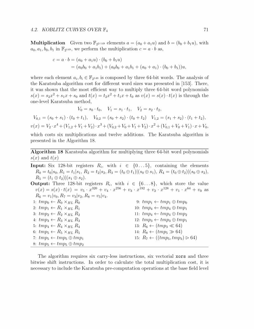
4.2. KOBLITZ CURVES OVER F4 71
Multiplication Given two F22·149 elements a = (a0 + a1u) and b = (b0 + b1u), witha0, a1, b0, b1 in F2149 , we perform the multiplication c = a · b as,
c = a · b = (a0 + a1u) · (b0 + b1u)
= (a0b0 + a1b1) + (a0b0 + a1b1 + (a0 + a1) · (b0 + b1))u,
where each element ai, bi ∈ F2149 is composed by three 64-bit words. The analysis ofthe Karatsuba algorithm cost for different word sizes was presented in [153]. There,it was shown that the most efficient way to multiply three 64-bit word polynomialss(x) = s2x
2 + s1x+ s0 and t(x) = t2x2 + t1x+ t0 as v(x) = s(x) · t(x) is through the
one-level Karatsuba method,
V0 = s0 · t0, V1 = s1 · t1, V2 = s2 · t2,
V0,1 = (s0 + s1) · (t0 + t1), V0,2 = (s0 + s2) · (t0 + t2) V1,2 = (s1 + s2) · (t1 + t2),
v(x) = V2 ·x4 +(V1,2 +V1 +V2) ·x3 +(V0,2 +V0 +V1 +V2) ·x2 +(V0,1 +V0 +V1) ·x+V0,
which costs six multiplications and twelve additions. The Karatsuba algorithm ispresented in the Algorithm 18.
Algorithm 18 Karatsuba algorithm for multiplying three 64-bit word polynomialss(x) and t(x)
Input: Six 128-bit registers Ri, with i ∈ {0 . . . 5}, containing the elementsR0 = t0|s0, R1 = t1|s1, R2 = t2|s2, R3 = (t0⊕ t1)|(s0⊕ s1), R4 = (t0⊕ t2)|(s0⊕ s2),R5 = (t1 ⊕ t2)|(s1 ⊕ s2).
Output: Three 128-bit registers Ri, with i ∈ {6 . . . 8}, which store the valuev(x) = s(x) · t(x) = v5 · x320 + v4 · x256 + v3 · x192 + v2 · x128 + v1 · x64 + v0 asR6 = v1|v0, R7 = v3|v2, R8 = v5|v4.
1: tmp0 ← R0 ×HL R0
2: tmp1 ← R1 ×HL R1
3: tmp2 ← R2 ×HL R2
4: tmp3 ← R3 ×HL R3
5: tmp4 ← R4 ×HL R4
6: tmp5 ← R5 ×HL R5
7: tmp5 ← tmp5 ⊕ tmp1
8: tmp5 ← tmp5 ⊕ tmp2
9: tmp1 ← tmp1 ⊕ tmp0
10: tmp4 ← tmp4 ⊕ tmp1
11: tmp4 ← tmp4 ⊕ tmp2
12: tmp3 ← tmp3 ⊕ tmp1
13: R6 ← (tmp3 � 64)14: R8 ← (tmp5 � 64)15: R7 ← ((tmp5, tmp3) B 64)
The algorithm requires six carry-less instructions, six vectorial xors and threebitwise shift instructions. In order to calculate the total multiplication cost, it isnecessary to include the Karatsuba pre-computation operations at the base field level

72 CHAPTER 4. KOBLITZ CURVES
(tweve vectorial xors and six byte interleaving instructions) and at the quadratic fieldlevel (six vectorial xors). Also, we must consider the reorganization of the registersin order to proceed with the modular reduction (six vectorial xors).
Modular reduction The modular reduction of an element a ∈ F22·149 takes ninevectorial xors and six bitwise shifts. The gains of the previously discussed registerconfiguration can be seen when we compare the reduction of quadratic field elements,presented in Algorithm 19 with the modular reduction of the base field elements (seeAlgorithm 16). The cost of reducing an element in F2149 in 64-bit registers is similarto the cost of the reduction of an element in F22·149 stored into 128-bit registers.Thus, we achieved the expected speedup of 100%.
Algorithm 19 Modular reduction of the terms a0, a1 of an element a = (a0 + a1u)modulo g(x) = x192 + x19 + 1
Input: An element a = a0 + a1u = (F ·x320 +E ·x256 +D ·x192 +C ·x128 +B ·x64 +A) + (L · x320 +K · x256 + J · x192 + I · x128 +H · x64 +G)u, with the 64-bit words(A-L) arranged in six 128-bit registers as R0 = G|A,R1 = H|B,R2 = I|C,R3 =J |D,R4 = K|E,R5 = L|F
Output: Elements (a0, a1) mod g(x) = M · x128 +N · x64 +O,P · x128 +Q · x64+R,with the 64-bit words (M-R) organized in three 128-bit registers asR6 = R|O,R7 = Q|N,R8 = P |M
1: R8 ← R2 ⊕R5
2: R7 ← R1 ⊕R4
3: R8 ← R8 ⊕ (R5 � 19)4: R7 ← R7 ⊕ (R4 � 19)5: R8 ← R8 ⊕ (R4 � 45)
6: R7 ← R7 ⊕ (R3 � 19)7: R6 ← R3 ⊕ (R5 � 45)8: R6 ← R6 ⊕ (R6 � 19)9: R6 ← R6 ⊕R0
Squaring Squaring is a very important function in the Koblitz curve point mul-tiplication algorithm, since it forms the building block for computing the τ endo-morphism. In our implementation, we computed the squaring operation throughcarry-less multiplication instructions which, experimentally, was less expensive thanthe bit interleaving method (see [78, Section 2.3.4]). The pre-processing phase isstraightforward, we just need to rearrange the 32-bit packed words of the 128-bitregisters in order to prepare them for the subsequent modular reduction.
The pre- and post-processing phases require three shuffle instructions, three vec-torial xors and three bitwise shifts. The complete function is described in Algo-rithm 20. Given 128-bit registers Ri, we depict the SSE 32-bit shuffle operation as
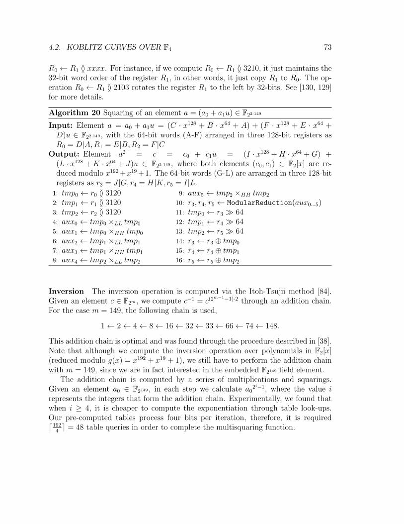
4.2. KOBLITZ CURVES OVER F4 73
R0 ← R1 G xxxx. For instance, if we compute R0 ← R1 G 3210, it just maintains the32-bit word order of the register R1, in other words, it just copy R1 to R0. The op-eration R0 ← R1 G 2103 rotates the register R1 to the left by 32-bits. See [130, 129]for more details.
Algorithm 20 Squaring of an element a = (a0 + a1u) ∈ F22·149
Input: Element a = a0 + a1u = (C · x128 + B · x64 + A) + (F · x128 + E · x64 +D)u ∈ F22·149 , with the 64-bit words (A-F) arranged in three 128-bit registers asR0 = D|A,R1 = E|B,R2 = F |C
Output: Element a2 = c = c0 + c1u = (I · x128 +H · x64 +G) +(L · x128 +K · x64 + J)u ∈ F22·149 , where both elements (c0, c1) ∈ F2[x] are re-duced modulo x192 +x19 +1. The 64-bit words (G-L) are arranged in three 128-bitregisters as r3 = J |G, r4 = H|K, r5 = I|L.
1: tmp0 ← r0 G 31202: tmp1 ← r1 G 31203: tmp2 ← r2 G 31204: aux0 ← tmp0 ×LL tmp0
5: aux1 ← tmp0 ×HH tmp0
6: aux2 ← tmp1 ×LL tmp1
7: aux3 ← tmp1 ×HH tmp1
8: aux4 ← tmp2 ×LL tmp2
9: aux5 ← tmp2 ×HH tmp2
10: r3, r4, r5 ← ModularReduction(aux0...5)11: tmp0 ← r3 � 6412: tmp1 ← r4 � 6413: tmp2 ← r5 � 6414: r3 ← r3 ⊕ tmp0
15: r4 ← r4 ⊕ tmp1
16: r5 ← r5 ⊕ tmp2
Inversion The inversion operation is computed via the Itoh-Tsujii method [84].Given an element c ∈ F2m , we compute c−1 = c(2m−1−1)·2 through an addition chain.For the case m = 149, the following chain is used,
1← 2← 4← 8← 16← 32← 33← 66← 74← 148.
This addition chain is optimal and was found through the procedure described in [38].Note that although we compute the inversion operation over polynomials in F2[x](reduced modulo g(x) = x192 + x19 + 1), we still have to perform the addition chainwith m = 149, since we are in fact interested in the embedded F2149 field element.
The addition chain is computed by a series of multiplications and squarings.Given an element a0 ∈ F2149 , in each step we calculate a0
2i−1, where the value irepresents the integers that form the addition chain. Experimentally, we found thatwhen i ≥ 4, it is cheaper to compute the exponentiation through table look-ups.Our pre-computed tables process four bits per iteration, therefore, it is requiredd192
4e = 48 table queries in order to complete the multisquaring function.
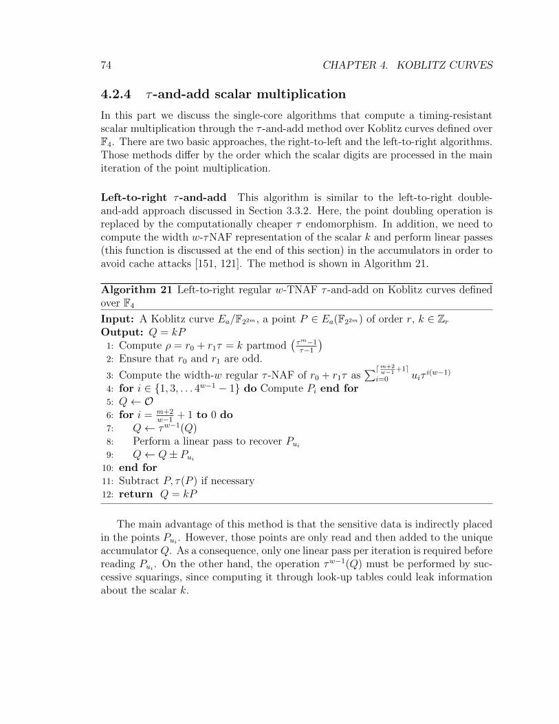
74 CHAPTER 4. KOBLITZ CURVES
4.2.4 τ-and-add scalar multiplication
In this part we discuss the single-core algorithms that compute a timing-resistantscalar multiplication through the τ -and-add method over Koblitz curves defined overF4. There are two basic approaches, the right-to-left and the left-to-right algorithms.Those methods differ by the order which the scalar digits are processed in the mainiteration of the point multiplication.
Left-to-right τ-and-add This algorithm is similar to the left-to-right double-and-add approach discussed in Section 3.3.2. Here, the point doubling operation isreplaced by the computationally cheaper τ endomorphism. In addition, we need tocompute the width w-τNAF representation of the scalar k and perform linear passes(this function is discussed at the end of this section) in the accumulators in order toavoid cache attacks [151, 121]. The method is shown in Algorithm 21.
Algorithm 21 Left-to-right regular w-TNAF τ -and-add on Koblitz curves definedover F4
Input: A Koblitz curve Ea/F22m , a point P ∈ Ea(F22m) of order r, k ∈ ZrOutput: Q = kP
1: Compute ρ = r0 + r1τ = k partmod(τm−1τ−1
)2: Ensure that r0 and r1 are odd.
3: Compute the width-w regular τ -NAF of r0 + r1τ as∑dm+2
w−1+1e
i=0 uiτi(w−1)
4: for i ∈ {1, 3, . . . 4w−1 − 1} do Compute Pi end for5: Q← O6: for i = m+2
w−1+ 1 to 0 do
7: Q← τw−1(Q)8: Perform a linear pass to recover Pui9: Q← Q± Pui
10: end for11: Subtract P, τ(P ) if necessary12: return Q = kP
The main advantage of this method is that the sensitive data is indirectly placedin the points Pui . However, those points are only read and then added to the uniqueaccumulator Q. As a consequence, only one linear pass per iteration is required beforereading Pui . On the other hand, the operation τw−1(Q) must be performed by suc-cessive squarings, since computing it through look-up tables could leak informationabout the scalar k.
4.2. KOBLITZ CURVES OVER F4 75
Right-to-left τ-and-add This other method processes the scalar k from the leastto the most significant digit. It is similar to the algorithm depicted in Chapter 3.In this case, the point halving is substituted by the τ endomorphism, and the GLVmethod is brought to its full extent, through the τ -adic representation of the scalark. This approach is presented in Algorithm 22.
Algorithm 22 Right-to-left regular w-TNAF τ -and-add on Koblitz curves definedover F4
Input: A Koblitz curve Ea/F22m , a point P ∈ Ea(F22m) of order r, k ∈ ZrOutput: Q = kP
1: Compute ρ = r0 + r1τ = k partmod (mod τm−1τ−1
)2: Ensure that r0 and r1 are odd.
3: Compute the width-w regular τ -NAF of r0 + r1τ as∑dm+2
w−1+1e
i=0 uiτi(w−1)
4: for i ∈ {1, 3, . . . 4w−1 − 1} do Qi = O5: for i = 0 to m+2
w−1+ 1 do
6: Perform a linear pass to recover Qui
7: Qui ← Qui ± P8: Perform a linear pass to store Qui
9: P ← τw−1(P )10: Q← O11: for i ∈ {1, 3, . . . 4w−1 − 1} do Q = i ·Qi
12: Subtract P, τ(P ) if necessary13: return Q = kP
Here, we have to perform a post-computation in the accumulators instead ofprecomputing the points Pi as in the previous approach. Also, the τ endomorphismis applied to the point P , which is usually public. For that reason, we can computeτ with table look-ups instead of performing squarings multiple times.
The downside of this algorithm is that the accumulators carry sensitive informa-tion about the digits of the scalar. Also, the accumulators are read and written. Asa result, it is necessary to apply the linear pass algorithm to the accumulators Qi
twice per iteration.
Linear pass The linear pass is a method designed to protect sensitive informationagainst side-channel attacks associated with the CPU cache access patterns. Letus consider an array A of size l. Before reading a value A[i], with i ∈ [0, l − 1],the linear pass technique reads the entire array A but only stores, possibly into anoutput register, the requested value A[i]. In that way, the attacker does not know
76 CHAPTER 4. KOBLITZ CURVES
which array index was accessed just by analyzing the location of the cache-miss in hisown artificially injected data. However, this method causes a considerable overhead,which depends on the size of the array.
In this work, we implemented the linear pass method using 128-bit SSE vectorialinstructions and registers. For each array index i, we copy it to a register and compareit with the current scalar k τNAF digit. The SSE instruction pcmpeqq compares thevalues of two 128-bit registers A and B and sets the resulting register C with bitsone, if A and B are equal, and bits zero otherwise. For that reason, we can use theregister C as a mask, which is applied to each value A[i] before copying it to theregister that will hold the requested data.
Experimental results shown that the implementation of the linear pass techniquewith SSE registers is more efficient than using 64-bit conditional move instructions[120] by an order of 2.125. Our approach is depicted in Algorithm 23.
Algorithm 23 Linear pass using 128-bit AVX vectorial instructions
Input: An array A of size l, a requested index i, SSE 128-bit registers tmp, dst.Output: The register dst containing A[d].
1: dst← 02: for i ∈ {0, . . . , l − 1} do3: tmp← i4: tmp← compare( tmp, i )
(compare returns 1128 if the operands are equal and 0128 otherwise.)5: tmp← tmp ∧ Pi6: dst← dst ∨ tmp7: end for
4.2.5 Results and discussion
Our software library can be executed in any Intel platform, which comes with theSSE4.1 vector instructions and the 64-bit carry-less multiplier instruction pclmulqdq.The benchmarking was executed in a Intel Core i7 4770k 3.50 GHz machine (Haswellarchitecture) with the TurboBoost and HyperThreading features disabled. Also, thelibrary was coded in the GNU11 C and Assembly languages.
Regarding the compilers, we performed an experimental analysis on the perfor-mance of our code compiled with different systems: GCC (Gnu Compiler Collection)versions 4.7, 4.8, 4.9, 5.1, 5.2; ICC (Intel C++ Compiler) version 15; and the clangfrontend for the LLVM compiler infrastructure versions 3.4 and 3.7. All compilations

4.2. KOBLITZ CURVES OVER F4 77
were done with the flags -O3 -march=core-avx27 -fomit-frame-pointer. For thesake of comparison, we reported our timings for all of the previously mentioned com-pilers. However, when comparing our code with the state-of-the-art works, we optedfor the clang/llvm 3.4, since it gave us the best performance.
Parameters Given q = 2m, with m = 149, we constructed our base binary fieldFq ∼= F2[x]/(f(x)) with the 69-term irreducible polynomial f(x) described in Sec-tion 4.2.3. The quadratic extension Fq2 ∼= Fq[u]/(h(u)) was built through the irre-ducible quadratic h(u) = u2+u+1. However, our base field arithmetic was computedmodulo the redundant trinomial g(x) = x192+x19+1, which has among its irreduciblefactors, the polynomial f(x).
Our Koblitz curve was defined over Fq2 as
E1/Fq2 : y2 + xy = x3 + ux2 + u,
and the group E1(Fq2) contains a subgroup of interest of order
r = 0x637845F7F8BFAB325B85412FB54061F148B7F6E79AE11CC843ADE1470F7E4E29,
which corresponds to approximately 255 bits. In addition, our scalar multiplicationwas computed using a base point P represented in lambda coordinates as
xP = 0x1B0CB55BC0B41C3EC1820E4E24EBC310451476
+ 0x4649A2FF1A1B8BA00AA8A706C04D6D97DF60C · u,λP = 0x6B64DFA496D1DEEA880545B44AC9CC4950C1C
+ 0x1ADB1DA167DBDF597F03D9A0889FF76FB0B2A1 · u.
Field and elliptic curve arithmetic timings In Table 4.7, we present the tim-ings for the base and the quadratic field arithmetic. The multisquaring operationis used to support the Itoh-Tsujii addition chain, therefore, is implemented only inF2149 (actually, in a 192-bit polynomial in F2[x]). In addition, we gave timings toreduce a 192-bit polynomial element in F2[x] modulo f(x). Finally, all timings ofoperations in the quadratic field include the subsequent modular reduction.
7For the ICC, instead of using -march-core-avx2, we used -xCORE-AVX2.
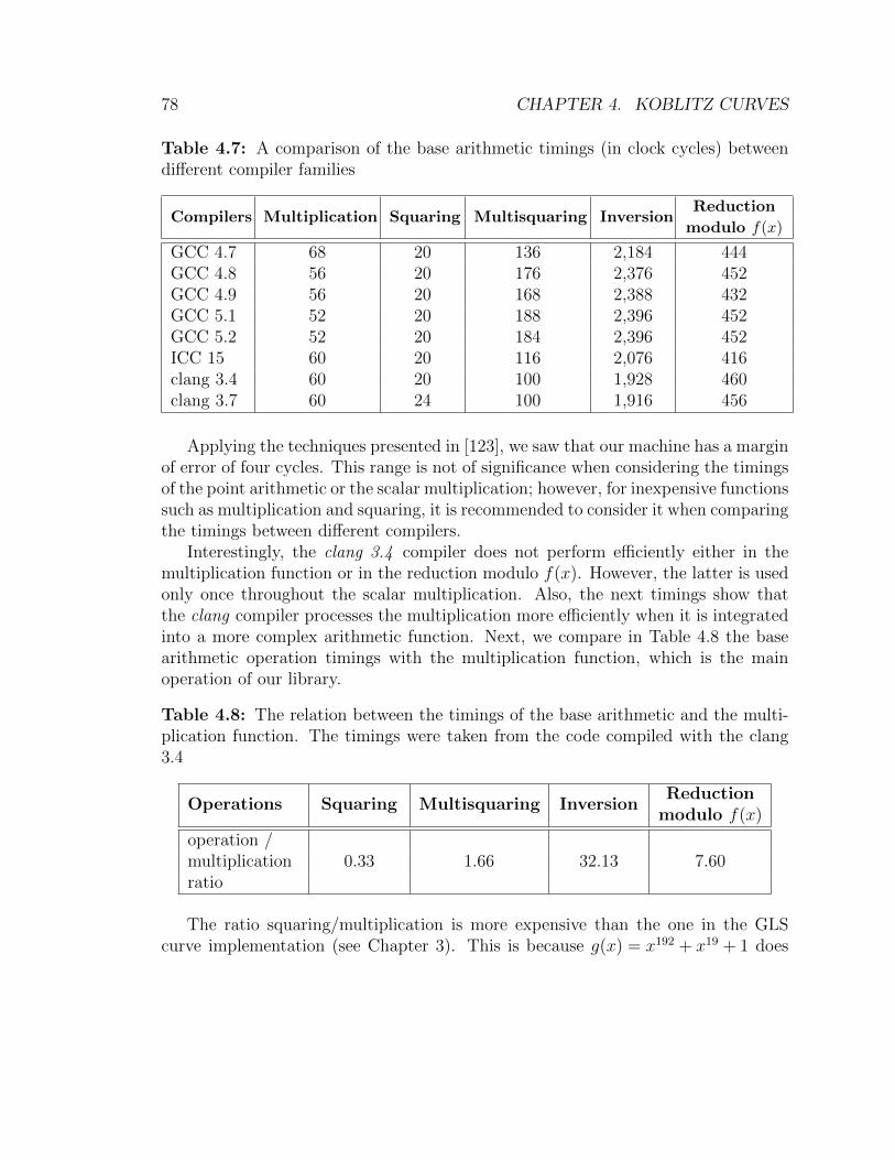
78 CHAPTER 4. KOBLITZ CURVES
Table 4.7: A comparison of the base arithmetic timings (in clock cycles) betweendifferent compiler families
Compilers Multiplication Squaring Multisquaring InversionReduction
modulo f(x)
GCC 4.7 68 20 136 2,184 444GCC 4.8 56 20 176 2,376 452GCC 4.9 56 20 168 2,388 432GCC 5.1 52 20 188 2,396 452GCC 5.2 52 20 184 2,396 452ICC 15 60 20 116 2,076 416clang 3.4 60 20 100 1,928 460clang 3.7 60 24 100 1,916 456
Applying the techniques presented in [123], we saw that our machine has a marginof error of four cycles. This range is not of significance when considering the timingsof the point arithmetic or the scalar multiplication; however, for inexpensive functionssuch as multiplication and squaring, it is recommended to consider it when comparingthe timings between different compilers.
Interestingly, the clang 3.4 compiler does not perform efficiently either in themultiplication function or in the reduction modulo f(x). However, the latter is usedonly once throughout the scalar multiplication. Also, the next timings show thatthe clang compiler processes the multiplication more efficiently when it is integratedinto a more complex arithmetic function. Next, we compare in Table 4.8 the basearithmetic operation timings with the multiplication function, which is the mainoperation of our library.
Table 4.8: The relation between the timings of the base arithmetic and the multi-plication function. The timings were taken from the code compiled with the clang3.4
Operations Squaring Multisquaring InversionReduction
modulo f(x)
operation /0.33 1.66 32.13 7.60multiplication
ratio
The ratio squaring/multiplication is more expensive than the one in the GLScurve implementation (see Chapter 3). This is because g(x) = x192 + x19 + 1 does
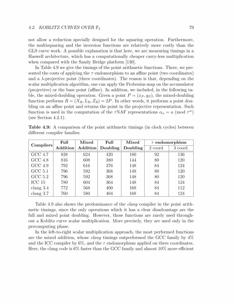
4.2. KOBLITZ CURVES OVER F4 79
not allow a reduction specially designed for the squaring operation. Furthermore,the multisquaring and the inversion functions are relatively more costly than theGLS curve work. A possible explanation is that here, we are measuring timings in aHaswell architecture, which has a computationally cheaper carry-less multiplicationwhen compared with the Sandy Bridge platform [130].
In Table 4.9 we give the timings of the point arithmetic functions. There, we pre-sented the costs of applying the τ endomorphism to an affine point (two coordinates)and a λ-projective point (three coordinates). The reason is that, depending on thescalar multiplication algorithm, one can apply the Frobenius map on the accumulator(projective) or the base point (affine). In addition, we included, in the following ta-ble, the mixed-doubling operation. Given a point P = (xP , yP ), the mixed-doublingfunction performs R = (XR, LR, ZR) = 2P . In other words, it performs a point dou-bling on an affine point and returns the point in the projective representation. Suchfunction is used in the computation of the τNAF representations αu = u (mod τw)(see Section 4.2.1).
Table 4.9: A comparison of the point arithmetic timings (in clock cycles) betweendifferent compiler families
CompilersFull Mixed Full Mixed τ endomorphism
Addition Addition Doubling Doubling 2 coord. 3 coord.
GCC 4.7 828 624 420 180 92 136GCC 4.8 816 608 380 144 80 120GCC 4.9 792 616 376 148 84 124GCC 5.1 796 592 368 148 80 120GCC 5.2 796 592 368 148 80 120ICC 15 780 604 364 148 84 124clang 3.4 772 568 400 168 84 112clang 3.7 760 580 404 168 84 124
Table 4.9 also shows the predominance of the clang compiler in the point arith-metic timings, since the only operations which it has a clear disadvantage are thefull and mixed point doubling. However, those functions are rarely used through-out a Koblitz curve scalar multiplication. More precisely, they are used only in theprecomputing phase.
In the left-to-right scalar multiplication approach, the most performed functionsare the mixed addition, whose clang timings outperformed the GCC family by 4%and the ICC compiler by 6%, and the τ endomorphism applied on three coordinates.Here, the clang code is 6% faster than the GCC family and almost 10% more efficient
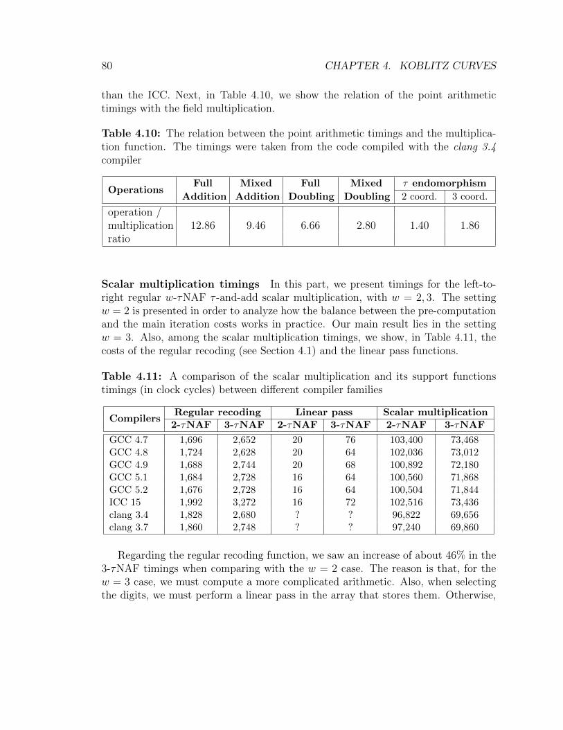
80 CHAPTER 4. KOBLITZ CURVES
than the ICC. Next, in Table 4.10, we show the relation of the point arithmetictimings with the field multiplication.
Table 4.10: The relation between the point arithmetic timings and the multiplica-tion function. The timings were taken from the code compiled with the clang 3.4compiler
OperationsFull Mixed Full Mixed τ endomorphism
Addition Addition Doubling Doubling 2 coord. 3 coord.
operation /12.86 9.46 6.66 2.80 1.40 1.86multiplication
ratio
Scalar multiplication timings In this part, we present timings for the left-to-right regular w-τNAF τ -and-add scalar multiplication, with w = 2, 3. The settingw = 2 is presented in order to analyze how the balance between the pre-computationand the main iteration costs works in practice. Our main result lies in the settingw = 3. Also, among the scalar multiplication timings, we show, in Table 4.11, thecosts of the regular recoding (see Section 4.1) and the linear pass functions.
Table 4.11: A comparison of the scalar multiplication and its support functionstimings (in clock cycles) between different compiler families
CompilersRegular recoding Linear pass Scalar multiplication2-τNAF 3-τNAF 2-τNAF 3-τNAF 2-τNAF 3-τNAF
GCC 4.7 1,696 2,652 20 76 103,400 73,468GCC 4.8 1,724 2,628 20 64 102,036 73,012GCC 4.9 1,688 2,744 20 68 100,892 72,180GCC 5.1 1,684 2,728 16 64 100,560 71,868GCC 5.2 1,676 2,728 16 64 100,504 71,844ICC 15 1,992 3,272 16 72 102,516 73,436clang 3.4 1,828 2,680 ? ? 96,822 69,656clang 3.7 1,860 2,748 ? ? 97,240 69,860
Regarding the regular recoding function, we saw an increase of about 46% in the3-τNAF timings when comparing with the w = 2 case. The reason is that, for thew = 3 case, we must compute a more complicated arithmetic. Also, when selectingthe digits, we must perform a linear pass in the array that stores them. Otherwise,
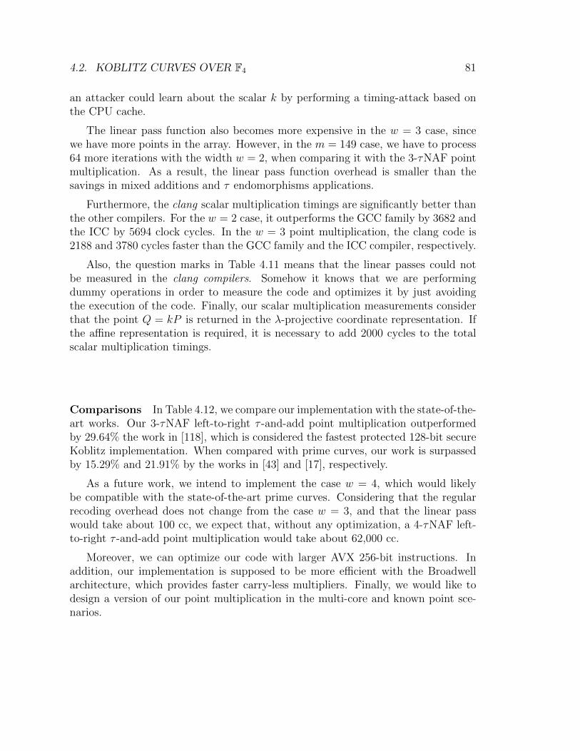
4.2. KOBLITZ CURVES OVER F4 81
an attacker could learn about the scalar k by performing a timing-attack based onthe CPU cache.
The linear pass function also becomes more expensive in the w = 3 case, sincewe have more points in the array. However, in the m = 149 case, we have to process64 more iterations with the width w = 2, when comparing it with the 3-τNAF pointmultiplication. As a result, the linear pass function overhead is smaller than thesavings in mixed additions and τ endomorphisms applications.
Furthermore, the clang scalar multiplication timings are significantly better thanthe other compilers. For the w = 2 case, it outperforms the GCC family by 3682 andthe ICC by 5694 clock cycles. In the w = 3 point multiplication, the clang code is2188 and 3780 cycles faster than the GCC family and the ICC compiler, respectively.
Also, the question marks in Table 4.11 means that the linear passes could notbe measured in the clang compilers. Somehow it knows that we are performingdummy operations in order to measure the code and optimizes it by just avoidingthe execution of the code. Finally, our scalar multiplication measurements considerthat the point Q = kP is returned in the λ-projective coordinate representation. Ifthe affine representation is required, it is necessary to add 2000 cycles to the totalscalar multiplication timings.
Comparisons In Table 4.12, we compare our implementation with the state-of-the-art works. Our 3-τNAF left-to-right τ -and-add point multiplication outperformedby 29.64% the work in [118], which is considered the fastest protected 128-bit secureKoblitz implementation. When compared with prime curves, our work is surpassedby 15.29% and 21.91% by the works in [43] and [17], respectively.
As a future work, we intend to implement the case w = 4, which would likelybe compatible with the state-of-the-art prime curves. Considering that the regularrecoding overhead does not change from the case w = 3, and that the linear passwould take about 100 cc, we expect that, without any optimization, a 4-τNAF left-to-right τ -and-add point multiplication would take about 62,000 cc.
Moreover, we can optimize our code with larger AVX 256-bit instructions. Inaddition, our implementation is supposed to be more efficient with the Broadwellarchitecture, which provides faster carry-less multipliers. Finally, we would like todesign a version of our point multiplication in the multi-core and known point sce-narios.
82 CHAPTER 4. KOBLITZ CURVES
Table 4.12: Scalar multiplication timings (in clock cycles) on 128-bit secure ellitpiccurves
Curve/Method TAR1 Architecture Timings
Koblitz over F2283 (NIST K-283)yes Haswell 99,000
τ -and-add, 5-τNAF [118]Twisted Edwards over F(2127−1)2 yes Haswell 59,000double-and-add [43]Kummer genus-2 over F2127−1 yes Haswell 54,389Kummer ladder [17]
Koblitz over F4149 yes Haswell 96,822τ-and-add, 2-τNAF (our work)Koblitz over F4149 yes Haswell 69,656τ-and-add, 3-τNAF (our work)1 Timing-attack resistant.
4.3 Summary
At first, we adapted the Joye-Tunstall recoding method to generate, for the firsttime, a timing-resistant τ -and-add scalar multiplication on Koblitz curves. Thisimplementation outperformed by 26% the protected Koblitz point multiplicationbased on the Montgomery ladder algorithm.
Next, we designed completely novel 128-bit secure scalar multiplication algo-rithms on Koblitz curves defined over F4. In order to achieve that, we implementeda fast base and quadratic field arithmetic, which took advantage of the redundanttrinomials method and allowed an efficient modular reduction.
Part II
The Discrete Logarithm Problem

5 | Finite Fields
Let FQ denote the finite field of order Q. The discrete logarithm problem (DLP) inFQ is that of determining, given a generator g of F∗Q and an element h ∈ F∗Q, theinteger x ∈ [0, Q − 2] satisfying h = gx. In the remainder of this chapter, we shallassume that the characteristic of FQ is 2 or 3.
Until recently, the fastest general-purpose algorithm known for solving the DLPin FQ was Coppersmith’s 1984 index-calculus algorithm [40] with a running time ofLQ[1
3, (32/9)1/3] ≈ LQ[1
3, 1.526], where as usual LQ[α, c] with 0 < α < 1 and c > 0
denotes the expression
exp((c+ o(1))(logQ)α(log logQ)1−α)
that is subexponential in logQ. In February 2013, Joux [86] presented a new DLPalgorithm with a running time of LQ[1
4+ o(1), c] (for some undetermined c) when
Q = q2n and q ≈ n. Shortly thereafter, Barbulescu, Gaudry, Joux and Thome [13]presented an algorithm with quasi-polynomial running time (logQ)O(log logQ) whenQ = q2n with q ≈ n.
These dramatic developments were accompanied by some striking computationalresults. For example, Gologlu et al. [68] computed logarithms in F28·3·255 = F26120
in only 750 CPU hours, and Joux [87] computed logarithms in F28·3·257 = F26168 inonly 550 CPU hours. The small computational effort expended in these experimentsdepends crucially on the special nature of the fields F26120 and F26168 — namely thatF26120 is a degree-255 extension of F28·3 with 255 = 28 − 1 (a Kummer extension),and F26168 is a degree-257 extension of F28·3 with 257 = 28 + 1 (a twisted Kummerextension). Adj et al. [2] presented a concrete analysis of the new algorithms anddemonstrated that logarithms in F36·509 can be computed in approximately 282 steps,which is considerably less than the 2128 steps required by Coppersmith’s algorithm.Unlike the aforementioned experimental results, the analysis by Adj et al. does notexploit any special properties of the fields F36·509 and F36·1429 .
The purpose of this work is to demonstrate that, with modest computational re-sources, the new algorithms can be used to solve instances of the discrete logarithm
85
86 CHAPTER 5. FINITE FIELDS
problem that remain beyond the reach of classical algorithms. The first target field isthe 1303-bit field F36·137 ; this field does not enjoy any Kummer-like properties. Moreprecisely, we are interested in solving the discrete logarithm problem in the order-rsubgroup G of F∗36·137 , where r = (3137 − 369 + 1)/7011427850892440647 is a 155-bitprime. The discrete logarithm problem in this group is of cryptographic interest be-cause the values of the bilinear pairing derived from the supersingular elliptic curveE : y2 = x3−x+ 1 over F3137 lie in G.1 Consequently, if logarithms in G can be com-puted efficiently then the associated bilinear pairing is rendered cryptographicallyinsecure. Note that since r is a 155-bit prime, Pollard’s rho algorithm [126] for com-puting logarithms in G is infeasible. Moreover, recent work on computing logarithmsin the 809-bit field F2809 [12] suggests that Coppersmith’s algorithm is infeasible forcomputing logarithms in G, whereas recent work on computing logarithms in the 923-bit field F36·97 [79] (see also [144]) indicates that computing logarithms in G using theJoux-Lercier algorithm [88] would be a formidable challenge. In contrast, we showthat Joux’s algorithm can be used to compute logarithms in G in just a few daysusing a small number of CPUs; more precisely, our computation consumed a total of888 CPU hours. The computational effort expended in our experiment is relativelysmall, despite the fact that our implementation was done using the computer algebrasystem Magma V2.20-2 [31] and is far from optimal.
The second target field is the 1551-bit field F36·163 ; this field does not enjoy anyKummer-like properties. More precisely, we are interested in solving the discretelogarithm problem in the order-r subgroup G of F∗36·163 , where r = 3163 + 382 + 1 isa 259-bit prime. The discrete logarithm problem in this group is of cryptographicinterest because the values of the bilinear pairing derived from the supersingularelliptic curve E : y2 = x3 − x − 1 over F3163 lie in G. This bilinear pairing wasfirst considered by Boneh, Lynn and Shacham in their landmark paper on shortsignature schemes [26]; see also [73]. Furthermore, the bilinear pairing derived fromthe quadratic twist of E was one of the pairings implemented by Galbraith, Harrisonand Soldera [59]. Again, we show that Joux’s algorithm can be used to computelogarithms in G in just a few days using a small number of CPUs; our computationused 1201 CPU hours.
After we had completed the F36·137 discrete logarithm computation, Granger,Kleinjung and Zumbragel [70] presented several practical improvements and refine-ments of Joux’s algorithm. These improvements allowed them to compute logarithmsin the 4404-bit field F212·367 in approximately 52,240 CPU hours, and drastically low-
1We note that the supersingular elliptic curves y2 = x3− x± 1 over F3n have embedding degree6 and were proposed for cryptographic use in several early papers on pairing-based cryptography[15, 26, 59, 72].
5.1. JOUX’S L[1/4 +O(1)] ALGORITHM 87
ered the estimated time to compute logarithms in the 4892-bit field F24·1223 to 259
modular multiplications. More recently, Joux and Pierrot [89] presented a more effi-cient algorithm for computing logarithms of factor base elements. The new algorithmwas used to compute logarithms in the 3796-bit characteristic-three field F35·479 inless than 8600 CPU hours.
Also, we present an analysis of the cost for solving the DLP in the characteristic-three fields F36·509 and F36·1429 . Both fields are used to construct k = 6 pairingsderived from supersingular elliptic curves Y 2 = X3 −X + 1 and Y 2 = X3 −X − 1over F3` considered in [26, 56, 15, 59] and implemented in [14, 72, 122, 6, 77, 24,34, 22]. Finally, we briefly discuss the practical implications of the quasi-polynomialalgorithm (QPA) of Barbulescu et al. [13] for solving the DLP in small-characteristicfields.
5.1 Joux’s L[1/4 + o(1)] algorithm
Let Fq3n be a finite field where n ≤ 2q + 1.2 The elements of Fq3n are representedas polynomials of degree at most n − 1 over Fq3 . Let N = q3n − 1, and let r be aprime divisor of N . In this work, we are interested in the discrete logarithm problemin the order-r subgroup of F∗q3n . More precisely, we are given two elements α, β oforder r in F∗q3n and we wish to find logα β. Let g be an element of order N in F∗q3n .Then logα β = (logg β)/(logg α) mod r. Thus, in the remainder of this section wewill assume that we need to compute logg h mod r, where h is an element of order rin F∗q3n .
The algorithm proceeds by first finding the logarithms (mod r) of all degree-oneelements in Fq3n (see Section 5.1.1). Then, in the descent stage, logg h is expressedas a linear combination of logarithms of degree-one elements. The descent stageproceeds in several steps, each expressing the logarithm of a degree-D element as alinear combination of the logarithms of elements of degree ≤ m for some m < D.Four descent methods are employed; these are described in Sections 5.1.2 – 5.1.5.
Notation. Nq3(m,n) denotes the number of monic m-smooth degree-n polynomialsin Fq3 [X], Aq3(m,n) denotes the average number of distinct monic irreducible factorsamong all monic m-smooth degree-n polynomials in Fq3 [X], and Sq3(m, d) denotesthe cost of testing m-smoothness of a degree-d polynomial in Fq3 [X]. Formulasfor Nq3(m,n), Aq3(m,n) and Sq3(m,n) are given in [2]. For γ ∈ Fq3 , γ denotes
the element γq2. For P ∈ Fq3 [X], P denotes the polynomial obtained by raising
2More generally, one could consider fields Fqkn where n ≤ 2q + 1. We focus on the case k = 3since our target fields are F36n with n ∈ {137, 163}, which we will embed in F(34)3·n .
88 CHAPTER 5. FINITE FIELDS
each coefficient of P to the power q2. The cost of an integer addition modulo ris denoted by Ar, and the cost of a multiplication in Fq3 is denoted by Mq3 . Theprojective general linear group of degree 2 over Fq is denoted PGL2(Fq). Pq is aset of distinct representatives of the left cosets of PGL2(Fq) in PGL2(Fq3); note that#Pq = q6 + q4 + q2. A matrix ( a bc d ) ∈ Pq is identified with the quadruple (a, b, c, d).
5.1.1 Setup
Select polynomials h0, h1 ∈ Fq3 [X] of small degree so that
X · h1(Xq)− h0(Xq) (5.1)
has an irreducible factor IX of degree n in Fq3 [X]; we will henceforth assume thatmax(deg h0, deg h1) = 2, whence n ≤ 2q + 1. Note that
X ≡ h0(Xq)
h1(Xq)≡(h0(X)
h1(X)
)q(mod IX). (5.2)
The field Fq3n is represented as Fq3n = Fq3 [X]/(IX) and the elements of Fq3n arerepresented as polynomials in Fq3 [X] of degree at most n− 1. Let g be a generatorof F∗q3n .
Finding logarithms of linear polynomials
Let B1 = {X + a | a ∈ Fq3}, and note that #B1 = q3. To compute the loga-rithms of B1-elements, we first generate linear relations of these logarithms. Let(a, b, c, d) ∈ Pq. Substituting Y 7→ (aX + b)/(cX + d) into the systematic equation
Y q − Y =∏α∈Fq
(Y − α) (5.3)
and using (5.2) yields((aX + b)(ch0 + d h1)− (ah0 + b h1)(cX + d)
)q(5.4)
≡ hq
1 · (cX + d) ·∏α∈Fq
[(a− αc)X + (b− αd)].
If the polynomial on the left side of (5.4) is 1-smooth, then taking logarithms (mod r)of both sides of (5.4) yields a linear relation of the logarithms of B1-elements and
5.1. JOUX’S L[1/4 +O(1)] ALGORITHM 89
the logarithm of h1. The probability that the left side of (5.4) is 1-smooth isNq3(1, 3)/q9 ≈ 1
6. Thus, after approximately 6q3 trials one expects to obtain q3
relations. The cost of the relation generation stage is 6q3 · Sq3(1, 3). The logarithmscan then be obtained by using Wiedemann’s algorithm for solving sparse systems oflinear equations [156, 41]. The expected cost of the linear algebra is q7 ·Ar since eachequation has approximately q nonzero terms.
5.1.2 Continued-fractions descent
Recall that we wish to compute logg h mod r, where h ∈ Fq3n = Fq3 [X]/(IX) hasorder r. We will henceforth assume that deg h = n − 1. The descent stage be-gins by multiplying h by a random power of g. The extended Euclidean algo-rithm is used to express the resulting field element h′ in the form h′ = w1/w2
where degw1, degw2 ≈ n/2 [83]; for simplicity, we shall assume that n is odd anddegw1 = degw2 = (n − 1)/2. This process is repeated until both w1 and w2 arem-smooth for some chosen m < (n − 1)/2. This gives logg h
′ as a linear combina-tion of logarithms of polynomials of degree at most m. The expected cost of thiscontinued-fractions descent step is approximately(
(q3)(n−1)/2
Nq3(m, (n− 1)/2)
)2
· Sq3(m, (n− 1)/2). (5.5)
The expected number of distinct irreducible factors of w1 and w2 is 2Aq3(m, (n−1)/2).In the concrete analysis, we shall assume that each of these irreducible factors hasdegree exactly m. The logarithm of each of these degree-m polynomials is thenexpressed as a linear combination of logarithms of smaller degree polynomials usingone of the descent methods described in Sections 5.1.3, 5.1.4 and 5.1.5.
5.1.3 Classical descent
Let p be the characteristic of Fq, and let q = p`. Let s ∈ [0, `], and let R ∈ Fq3 [X, Y ].Then it can be seen that[
R(X, (h0/h1)p`−s
)]ps≡ R′(Xps , X) (mod IX) (5.6)
where R′ is obtained from R by raising all its coefficients to the power ps. Letµ = degY R. Then multiplying both sides of (5.6) by h
qµ
1 gives[hp`−s·µ1 ·R(X, (h0/h1)p
`−s)]ps≡ h
qµ
1 ·R′(Xps , X) (mod IX). (5.7)
90 CHAPTER 5. FINITE FIELDS
Let Q ∈ Fq3 [X] with degQ = D, and let m < D. In the Joux-Lercier descentmethod [88], as modified by Gologlu et al. [67], one selects s ∈ [0, `] and searches fora polynomial R ∈ Fq3 [X, Y ] such that (i) Q | R2 where R2 = R′(Xps , X); (ii) degR1
and degR2/Q are appropriately balanced where R1 = hp`−sµ
1 R(X, (h0/h1)p`−s
); and(iii) both R1 and R2/Q are m-smooth. Taking logarithms of both sides of (5.7) thengives an expression for loggQ in terms of the logarithms of polynomials of degree atmost m.
A family of polynomials R satisfying (i) and (ii) can be constructed by finding abasis {(u1, u2), (v1, v2)} of the lattice
LQ = {(w1, w2) ∈ Fq3 [X]× Fq3 [X] : Q | (w1(X)− w2(X)Xps)}
where deg u1, deg u2, deg v1, deg v2 ≈ D/2. By writing (w1, w2) = a(u1, u2) +b(v1, v2) = (au1 + bv1, au2 + bv2) with a ∈ Fq3 [X] monic of degree δ and b ∈ Fq3 [X]of degree δ − 1, the points (w1, w2) in LQ can be sampled to obtain polynomi-als R(X, Y ) = w′′1(Y ) − w′′2(Y )X satisfying (i) and (ii) where w′′ is obtained fromw by raising all its coefficients to the power p−s. The number of lattice pointsto consider is therefore (q3)2δ. We have degw1, degw2 ≈ D/2 + δ, so degR1 =t1 ≈ 2(D/2 + δ)p`−s + 1 and degR2 = t2 ≈ (D/2 + δ) + ps. In order to ensure thatthere are sufficiently many such lattice points to generate a polynomial R for whichboth R1 and R2/Q are m-smooth, the parameters s and δ must be selected so that
q6δ � q3t1
Nq3(m, t1)· q3(t2−D)
Nq3(m, t2 −D). (5.8)
Ignoring the time to compute a balanced basis of LQ, the expected cost of finding apolynomial R satisfying (i)–(iii) is
q3t1
Nq3(m, t1)· q3(t2−D)
Nq3(m, t2 −D)·min(Sq3(m, t1), Sq3(m, t2 −D)). (5.9)
The expected number of distinct irreducible factors of R1 and R2/Q is Aq3(m, t1) +Aq3(m, t2 −D).
5.1.4 Grobner bases descent
Let Q ∈ Fq3 [X] with degQ = D. Let m = d(D + 1)/2e, and suppose that 3m < n.In Joux’s new descent method [86, Section 5.3], one finds degree-m polynomials
k1, k2 ∈ Fq3 [X] such that G = k1k2 − k1k2 = QR, where k1 = hm
1 k1(h0/h1) and
5.1. JOUX’S L[1/4 +O(1)] ALGORITHM 91
k2 = hm
1 k2(h0/h1), and R ∈ Fq3 [X]. Note that degR = 3m−D. If R is m-smooth,then we obtain a linear relationship between loggQ and logs of degree-m polynomials(see [4, Section 3.7]):
hmq
1 · k2 ·∏α∈Fq
(k1 − αk2) ≡ (Q(X)R(X))q (mod IX). (5.10)
To determine (k1, k2, R) that satisfy
k1k2 − k1k2 = QR, (5.11)
one can transform (5.11) into a system of multivariate quadratic equations over Fq.Specifically, each coefficient of k1, k2 and R is written using three variables over Fq.The coefficients of k1 and k2 can then be written in terms of the coefficients of k1 andk2. Hence, equating coefficients of X i of both sides of (5.11) yields 3m+ 1 quadraticequations. Equating Fq-components of these equations then yields 9m + 3 bilinearequations in 15m− 3D+ 9 variables over Fq. This system of equations can be solvedby finding a Grobner basis for the ideal it generates. Finally, solutions (k1, k2, R)are tested until one is found for which R is m-smooth. This yields an expressionfor loggQ in terms of the logarithms of approximately q + 1 + Aq3(m, 3m − D)polynomials of degree (at most) m; in the concrete analysis we shall assume thateach of the polynomials has degree exactly m.
5.1.5 2-to-1 descent.
The Grobner bases descent methodology of §2.5 can be employed in the case (D,m) =(2, 1). However, as also reported by Joux in his F26168 discrete log computation [87],we found the descent to be successful for only about 50% of all irreducible quadraticpolynomials. Despite this, some strategies can be used to increase this percentage.
Let Q(X) = X2 + uX + v ∈ Fq3 [X] be an irreducible quadratic polynomial forwhich the Grobner bases descent method failed.
Strategy 1. Introduced by Joux [87] and Gologlu et al. [68], this strategy is basedon the systematic equation derived from Y q′ − Y where q′ < q and Fq′ is a propersubfield of Fq3 instead of the systematic equation (5.3) derived from Y q − Y . Let pbe the characteristic of Fq, and let q = p`, q′ = p`
′, and s = `− `′. Then q = ps · q′.
Now, one searches for a, b, c, d ∈ Fq3 such that
G = (aX + b)(ch0 + d h1)ps − (ah0 + b h1)p
s
(cX + d) = QR

92 CHAPTER 5. FINITE FIELDS
with R ∈ Fq3 [X]. Note that degR = 2ps − 1.3 If R is 1-smooth, then we obtain alinear relationship between loggQ and logs of linear polynomials since
Gq ≡ hpsq
1 · (cX + d)ps ·∏α∈Fq′
((aX + b)p
s − α(cX + d)ps)
(mod IX),
as can be seen by making the substitution Y 7→ (aX + b)ps/(cX + d)p
sinto the
systematic equation derived from Y q′ − Y .Unfortunately, in all instances we considered, the polynomial R never factors
completely into linear polynomials. However, it hopefully factors into a quadraticpolynomial Q′ and 2ps− 3 linear polynomials, thereby yielding a relation between Qand another quadratic which has a roughly 50% chance of descending using Grobnerbases descent. Combined with the latter, this strategy descends about 95% of allirreducible quadratic polynomials in the fields F36·137 and F36·163 .
Strategy 2. We have
h2q
1 Q(X) ≡ h2q
1 Q((h0/h1)q) = h2q
0 + uhq
0hq
1 + vh2q
1
= (h2
0 + uh0h1 + v h2
1)q (mod IX). (5.12)
It can be seen that the degree-4 polynomial fQ(X) = h2
0 + uh0h1 + v h2
1 is either aproduct of two irreducible quadratics or itself irreducible. In the former case, weapply the standard Grobner bases descent method to the two irreducible quadratics.If both descents are successful, then we have succeeded in descending the original Q.
The strategies are combined in the following manner. For an irreducible quadraticQ ∈ Fq3 [X], we first check if the Grobner bases descent is successful. If the descentfails, we apply Strategy 2 to Q. In the case where fQ factors into two irreduciblequadratics, and at least one of them fails to descent with Grobner bases descent, weapply Strategy 1 to Q. If Strategy 1 fails on Q, we apply it to the two quadraticfactors of fQ. In the case where fQ is irreducible, we apply Strategy 1 to Q.
If none of the attempts succeed, we declare Q to be “bad”, and avoid it in thehigher-degree descent steps by repeating a step until all the quadratics encounteredare “good”. In our experiments with F36·137 and F36·163 , we observed that approxi-mately 97.2% of all irreducible quadratic polynomials Q were “good”.
3For our F36·137 and F36·163 computations, we have q = 34 and used q′ = 33, so s = 1 anddegR = 5.
5.2. COMPUTING DISCRETE LOGARITHMS IN F36·137 93
To see that this percentage is sufficient to complete the descent phase in thesetwo fields, consider a 3-to-2 descent step where the number of resulting irreduciblequadratic polynomials is 42 on average (cf. equation (5.10)). Then the probabilityof descending a degree-3 polynomial after finding one useful solution (k1, k2, R) inGrobner bases descent is 0.97242 ≈ 0.3. Therefore, after at most four trials we expectto successfully descend a degree-3 polynomial. Since the expected number of distinctsolutions of (5.11) is approximately q3 (according to equation (10) in [70]), one canafford this many trials.
5.2 Computing discrete logarithms in F36·137
The supersingular elliptic curve E : y2 = x3−x+ 1 has order #E(F3137) = cr, where
c = 7 · 4111 · 5729341 · 42526171
and
r = (3137 − 369 + 1)/c = 33098280119090191028775580055082175056428495623
is a 155-bit prime [23]. The Weil and Tate pairing attacks [112, 55] efficiently reducethe discrete logarithm problem in the order-r subgroup E of E(F3137) to the discretelogarithm problem in the order-r subgroup G of F∗36·137 .
Our approach to computing logarithms in G is to use Joux’s algorithm to computelogarithms in the quadratic extension F312·137 of F36·137 (so q = 34 and n = 137 inthe notation of Section 5.1). More precisely, we are given two elements α, β of orderr in F∗312·137 and we wish to find logα β. Let g be a generator of F∗312·137 . Thenlogα β = (logg β)/(logg α) mod r. Thus, in the remainder of the section we willassume that we need to compute logg h mod r, where h is an element of order r inF∗312·137 .
The DLP instance we solved is described in Section 5.2.1. The concrete esti-mates from Section 5.1 for solving the DLP instances are given in Section 5.2.2.These estimates are only upper bounds on the running time of the algorithm. Never-theless, they provide convincing evidence for the feasibility of the discrete logarithmcomputations. Our experimental results are presented in Section 5.2.3.
5.2.1 Problem instance
Let N denote the order of F∗312·137 . Using the tables from the Cunningham Project[134], we determined that the factorization of N is N = p4
1 ·∏31
i=2 pi, where the pi are

94 CHAPTER 5. FINITE FIELDS
the following primes (and r = p25):
p1 = 2 p2 = 5 p3 = 7 p4 = 13 p5 = 73 p6 = 823 p7 = 4111 p8 = 4933
p9 = 236737 p10 = 344693 p11 = 2115829 p12 = 5729341 p13 = 42526171
p14 = 217629707 p15 = 634432753 p16 = 685934341 p17 = 82093596209179
p18 = 4354414202063707 p19 = 18329390240606021 p20 = 46249052722878623693
p21 = 201820452878622271249 p22 = 113938829134880224954142892526477
p23 = 51854546646328186791017417700430486396513
p24 = 273537065683369412556888964042827802376371
p25 = 33098280119090191028775580055082175056428495623
p26 = 706712258201940254667826642673008768387229115048379
p27 = 108081809773839995188256800499141543684393035450350551
p28 = 91321974595662761339222271626247966116126450162880692588587183952237
p29 = 39487531149773489532096996293368370182957526257988573877031054477249
393549
p30 = 40189860022384850044254854796561182547553072730738823866986300807613
29207749418522920289
p31 = 19064323153825272072803685870803955622834286523139037403580752310822
7896644646984063736942624066227406898132113366226593158464419713.
We chose F34 = F3[U ]/(U4 + U2 + 2) and F312 = F34 [V ]/(V 3 + V + U2 + U),and selected h0(X) = V 326196X2 + V 35305X + V 204091 ∈ F312 [X] and h1 = 1. ThenIX ∈ F312 [X] is the degree-137 monic irreducible factor of X − h0(X34); the otherirreducible factor has degree 25.
We chose the generator g = X+V 113713 of F∗312·137 . To generate an order-r discretelogarithm challenge h, we computed
h′ =136∑i=0
(V bπ·(3
12)i+1c mod 312)X i
and then set h = (h′)N/r. The discrete logarithm logg h mod r was found to be
x = 27339619076975093920245515973214186963025656559.
This can be verified by checking that h = (gN/r)y, where y = x · (N/r)−1 mod r.
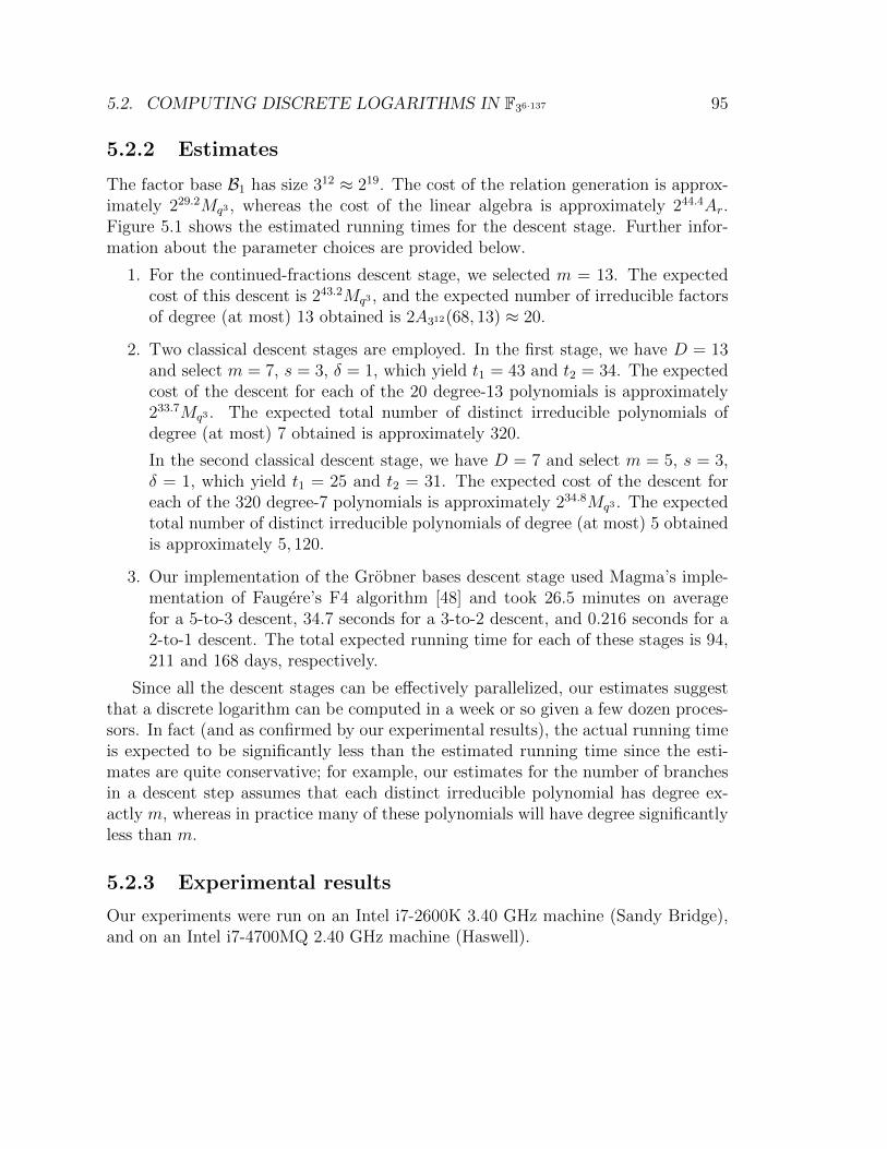
5.2. COMPUTING DISCRETE LOGARITHMS IN F36·137 95
5.2.2 Estimates
The factor base B1 has size 312 ≈ 219. The cost of the relation generation is approx-imately 229.2Mq3 , whereas the cost of the linear algebra is approximately 244.4Ar.Figure 5.1 shows the estimated running times for the descent stage. Further infor-mation about the parameter choices are provided below.
1. For the continued-fractions descent stage, we selected m = 13. The expectedcost of this descent is 243.2Mq3 , and the expected number of irreducible factorsof degree (at most) 13 obtained is 2A312(68, 13) ≈ 20.
2. Two classical descent stages are employed. In the first stage, we have D = 13and select m = 7, s = 3, δ = 1, which yield t1 = 43 and t2 = 34. The expectedcost of the descent for each of the 20 degree-13 polynomials is approximately233.7Mq3 . The expected total number of distinct irreducible polynomials ofdegree (at most) 7 obtained is approximately 320.
In the second classical descent stage, we have D = 7 and select m = 5, s = 3,δ = 1, which yield t1 = 25 and t2 = 31. The expected cost of the descent foreach of the 320 degree-7 polynomials is approximately 234.8Mq3 . The expectedtotal number of distinct irreducible polynomials of degree (at most) 5 obtainedis approximately 5, 120.
3. Our implementation of the Grobner bases descent stage used Magma’s imple-mentation of Faugere’s F4 algorithm [48] and took 26.5 minutes on averagefor a 5-to-3 descent, 34.7 seconds for a 3-to-2 descent, and 0.216 seconds for a2-to-1 descent. The total expected running time for each of these stages is 94,211 and 168 days, respectively.
Since all the descent stages can be effectively parallelized, our estimates suggestthat a discrete logarithm can be computed in a week or so given a few dozen proces-sors. In fact (and as confirmed by our experimental results), the actual running timeis expected to be significantly less than the estimated running time since the esti-mates are quite conservative; for example, our estimates for the number of branchesin a descent step assumes that each distinct irreducible polynomial has degree ex-actly m, whereas in practice many of these polynomials will have degree significantlyless than m.
5.2.3 Experimental results
Our experiments were run on an Intel i7-2600K 3.40 GHz machine (Sandy Bridge),and on an Intel i7-4700MQ 2.40 GHz machine (Haswell).

96 CHAPTER 5. FINITE FIELDS
Continued fraction descentTime: 243.2Mq3
68 (2)
Classical descent
7 (320)Classical descentTime: 320 · 234.8Mq3
Time: 20 · 233.7Mq3
13 (20)
5 (5,120)Grobner bases descentTime: 5, 120 · (26.5 minutes)
3 (219)
Time: 219 · (34.7 seconds)Grobner bases descent
1
2 (226)Grobner bases descentTime: 226 · (0.216 seconds)
Figure 5.1: A typical path of the descent tree for computing an individual logarithmin F312·137 (q = 34). The numbers in parentheses next to each node are the expectednumber of nodes at that level. ‘Time’ is the expected time to generate all nodes ata level.
5.3. COMPUTING DISCRETE LOGARITHMS IN F36·163 97
Relation generation took 1.05 CPU hours (Sandy Bridge, 1 core). The resultingsparse linear system of linear equation was solved using Magma’s multi-threadedparallel version of the Lanczos algorithm; the computation took 556.8 CPU hours(Sandy Bridge, 4 cores).
In the continued-fractions descent stage, the first degree-68 polynomial yielded 9irreducible factors of degrees 12, 12, 11, 10, 8, 6, 6, 2, 1, and the second degree-68polynomial yielded 11 irreducible factors of degrees 13, 12, 10, 10, 7, 6, 5, 2, 1, 1, 1.The computation took 22 CPU hours (Haswell, 4 cores).
Classical descent was used on the 9 polynomials of degree ≥ 8 to obtain polyno-mials of degree ≤ 7, and then on the 23 polynomials of degree 7 and 23 polynomialsof degree 6 to obtain polynomials of degree ≤ 5. These computations took 80 CPUhours (Haswell, 4 cores).
Finally, we used 5-to-3, 4-to-3, 3-to-2 and 2-to-1 Grobner bases descent proce-dures. The average time for a 4-to-3 descent was 33.8 seconds; the other averagetimes are given in Figure 5.1. In total, we performed 233 5-to-3 descents, 174 4-to-3descents, and 11573 3-to-2 descents. These computations took 115.2 CPU hours,1.5 CPU hours, and 111.2 CPU hours, respectively (Haswell, 4 cores). We also per-formed 493537 2-to-1 descents; their running times are incorporated into the runningtimes for the higher-level descents.
5.3 Computing discrete logarithms in F36·163
The supersingular elliptic curve E : y2 = x3 − x − 1 has order #E(F3163) = 3163 +382 + 1 = r, where r is the following 259-bit prime:
r = 589881151426658740854227725580736348850640632297373414091790995505756
623268837.
The Weil and Tate pairing attacks [112, 55] efficiently reduce the discrete logarithmproblem in the order-r group E = E(F3163) to the discrete logarithm problem in theorder-r subgroup G of F∗36·163 .
As in Section 5.2, we will compute logarithms in G by using Joux’s algorithmto compute logarithms in the quadratic extension F312·163 of F36·163 (so q = 34 andn = 163 in the notation of Section 5.1). We will compute logg h mod r, where g is agenerator of F∗312·163 and h is an element of order r in F∗312·163 .

98 CHAPTER 5. FINITE FIELDS
5.3.1 Problem instance
Let N denote the order of F∗312·163 . Using the tables from the Cunningham Project[134], we partially factored N as N = C · p4
1 ·∏22
i=2 pi, where the pi are the followingprimes (and r = p20):
p1 = 2 p2 = 5 p3 = 7 p4 = 13 p5 = 73 p6 = 653 p7 = 50857
p8 = 107581 p9 = 489001 p10 = 105451873 p11 = 380998157
p12 = 8483499631 p13 = 5227348213873 p14 = 8882811705390167
p15 = 4956470591980320134353 p16 = 23210817035829275705929
p17 = 3507171060957186767994912136200333814689659449
p18 = 6351885141964057411259499526611848626072045955243
p19 = 84268735918094105836318246511533764121140010481130741067443071103148
817701717
p20 = 58988115142665874085422772558073634885064063229737341409179099550575
6623268837
p21 = 13262905784043723370034025667618121081540438283177268680045186884853
26204127242781054287716913828905695771535319617625904849821802388801
p22 = 24879984727675011205198718183055547601122582974374576908898869641570
09269122423985704395925964922959410448009886539842494955927136450643
31019158574269,
and C is the following 919-bit composite number
C = 2873322036656120507394501949912283436722983546265951551507632957325767
0275216328747773792566523729655097848102113488795698936768394494992621
2312022819011019340957620502000045691081669475648919901346991751981450
8311534570945558522228827298337826215043744094861514754454151493177.
We verified that gcd(C,N/C) = 1 and that C is not divisible by any of the first 107
primes. Consequently, if an element g is selected uniformly at random from F∗312·163 ,and g satisfies g(N−1)/pi 6= 1 for 1 ≤ i ≤ 22, then g is a generator with very highprobability.4
We chose F34 = F3[U ]/(U4 + U2 + 2) and F312 = F34 [V ]/(V 3 + V + U2 + U), andselected h0(X) = 1 and
h1(X) = X2 + V 530855 ∈ F312 [X].
4More precisely, since C has at most 34 prime factors, each of which is greater than the primep = 179424673, the probability that g is a generator is at least (1− 1
p )34 > 0.99999981.
5.3. COMPUTING DISCRETE LOGARITHMS IN F36·163 99
Then IX ∈ F312 [X] is the degree-163 irreducible polynomial X · h1(X34)− 1:
IX = X163 + V 530855X + 2.
We chose g = X + V 2, which we hope is a generator of F∗312·163 .To generate an order-r discrete logarithm challenge h, we computed
h′ =162∑i=0
(V bπ·(3
12)i+1c mod 312)X i
and then set h = (h′)N/r. The discrete logarithm logg h mod r was found to be
x = 42639595149827919371329139195344900073259255425113252567203978435605
4526194343.
This can be verified by checking that h = (gN/r)y, where y = x · (N/r)−1 mod r.
5.3.2 Experimental results
Our experiments were run on an Intel i7-2600K 3.40 GHz machine (Sandy Bridge),and on an Intel Xeon E5-2650 2.00 GHz machine (Sandy Bridge-EP). The descentstrategy was similar to the one used for the F36·137 computation.
Relation generation took 0.84 CPU hours (Sandy Bridge, 1 core). The resultingsparse system of linear equations was solved using Magma’s multi-threaded parallelversion of the Lanczos algorithm; the computation took 852.5 CPU hours (SandyBridge, 4 cores).
In the continued-fractions descent stage with m = 15, the first degree-81 polyno-mial yielded 8 irreducible factors of degrees 15, 15, 14, 14, 10, 7, 5, 1, and the seconddegree-81 polynomial yielded 12 irreducible factors of degrees 12, 10, 9, 9, 9, 8, 6, 6,6, 4, 1, 1. The computation took 226.7 CPU hours (Sandy Bridge-EP, 16 cores).
Classical descent was used on the 11 polynomials of degree ≥ 8 to obtain polyno-mials of degree ≤ 7, and then a variant of classical descent (called the “alternative”method in Section 3.5 of [4]) was used on the 15 polynomials of degree 7 and 30polynomials of degree 6 to obtain polynomials of degree ≤ 5. These computationstook 51.0 CPU hours (Sandy Bridge-EP, 16 cores).
Finally, we used 5-to-3, 4-to-3 and 3-to-2 Grobner bases descent procedures. Thedescent was sped up by writing the coefficients of R (cf. equation (5.11)) in termsof the coefficients of k1 and k2; this reduced the number of variables in the resultingbilinear equations from 15m − 3D + 9 to 9m + 3. In total, we performed 213 5-to-3 descents, 187 4-to-3 descents, and 11442 3-to-2 descents. These computations

100 CHAPTER 5. FINITE FIELDS
took 24.0 CPU hours (Sandy Bridge-EP 16 cores), 0.8 CPU hours (Sandy Bridge, 4cores), and 44.8 CPU hours (Sandy Bridge, 4 cores), respectively. The running timesof the 2-to-1 descents were incorporated into the running times for the higher-leveldescents.
5.4 Higher extension degrees
As mentioned in the introduction of this chapter, there have been several practical im-provements and refinements in discrete logarithm algorithms since Joux’s L[1
4+o(1)]
algorithm. Most notably, Granger, Kleinjung and Zumbragel [70] presented severalrefinements that allowed them to compute logarithms in the 4404-bit characteristic-two field F212·367 , and Joux and Pierrot [89] presented a faster algorithm for computinglogarithms of factor base elements and used it to compute logarithms in the 3796-bitcharacteristic-three field F35·479 .
In Section 5.4.1, we show that the techniques from [89] and [70] can be usedto lower the estimate from [2] for computing discrete logarithms in the 4841-bitcharacteristic-three field F36·509 from 281.7Mq2 to 258.9Mq (where q = 36). In Section5.4.2, we use techniques from [70] to lower the estimate from [4] for computingdiscrete logarithms in the 13590-bit characteristic-three field F36·1429 from 295.8Mq2
to 278.8Mq2 (where q = 36). We emphasize that these estimates are upper boundson the running times of known algorithms for computing discrete logarithms. Ofcourse, it is possible that these upper bounds can be lowered with a more judiciouschoice of algorithm parameters, or with a tighter analysis, or with improvements tothe algorithms themselves.
5.4.1 Computing discrete logarithms in F36·509.
As in Section 4 of [2], we are interested in computing discrete logarithms in the orderr-subgroup of F∗36·509 , where r = (3509 − 3255 + 1)/7 is an 804-bit prime.
We use the algorithm developed by Joux and Pierrot [89], whence q = 36 andk = 1. The field F36 is represented as F3[u]/(u6 + 2u4 + u2 + 2u + 2). The fieldF36·509 is represented as F36 [X]/(IX), where IX is the degree-509 irreducible factorof h1(X)Xq − h0(X) with h0(X) = u46X + u219 and h1(X) = X(X + u409). Jouxand Pierrot [89] exploit the special form of h0(X) and h1(X) to accelerate the com-putation of logarithms of polynomials of degree ≤ 4; the dominant step is the com-putation of logarithms of degree-3 polynomials, where q linear algebra problems aresolved each taking time approximately q5/27Ar. The continued-fractions, classicaland Grobner bases descents are all performed over Fq.
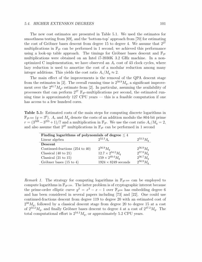
5.4. HIGHER EXTENSION DEGREES 101
The new cost estimates are presented in Table 5.1. We used the estimates forsmoothness testing from [69], and the ‘bottom-top’ approach from [70] for estimatingthe cost of Grobner bases descent from degree 15 to degree 4. We assume that 227
multiplications in F36 can be performed in 1 second; we achieved this performanceusing a look-up table approach. The timings for Grobner bases descent and F36
multiplications were obtained on an Intel i7-3930K 3.2 GHz machine. In a non-optimized C implementation, we have observed an Ar cost of 43 clock cycles, wherelazy reduction is used to amortize the cost of a modular reduction among manyinteger additions. This yields the cost ratio Ar/Mq ≈ 2.
The main effect of the improvements is the removal of the QPA descent stagefrom the estimates in [2]. The overall running time is 258.9Mq, a significant improve-ment over the 281.7Mq2 estimate from [2]. In particular, assuming the availability ofprocessors that can perform 227 F36-multiplications per second, the estimated run-ning time is approximately 127 CPU years — this is a feasible computation if onehas access to a few hundred cores.
Table 5.1: Estimated costs of the main steps for computing discrete logarithms inF36·509 (q = 36). Ar and Mq denote the costs of an addition modulo the 804-bit primer = (3509−3255 + 1)/7 and a multiplication in F36 . We use the cost ratio Ar/Mq = 2,and also assume that 227 multiplications in F36 can be performed in 1 second
Finding logarithms of polynomials of degree ≤ 4Linear algebra 252.3Ar 253.3Mq
DescentContinued-fractions (254 to 40) 256.9Mq 256.9Mq
Classical (40 to 21) 12.7× 254.2Mq 257.9Mq
Classical (21 to 15) 159× 249.4Mq 256.7Mq
Grobner bases (15 to 4) 1924× 8249 seconds 250.9Mq
Remark 1. The strategy for computing logarithms in F36·509 can be employed tocompute logarithms in F36·239 . The latter problem is of cryptographic interest becausethe prime-order elliptic curve y2 = x3 − x − 1 over F3239 has embedding degree 6and has been considered in several papers including [73] and [22]. One could usecontinued-fractions descent from degree 119 to degree 20 with an estimated cost of250Mq, followed by a classical descent stage from degree 20 to degree 15 at a costof 253.2Mq, and finally Grobner bases descent to degree 4 at a cost of 247.2Mq. Thetotal computational effort is 254.3Mq, or approximately 5.2 CPU years.
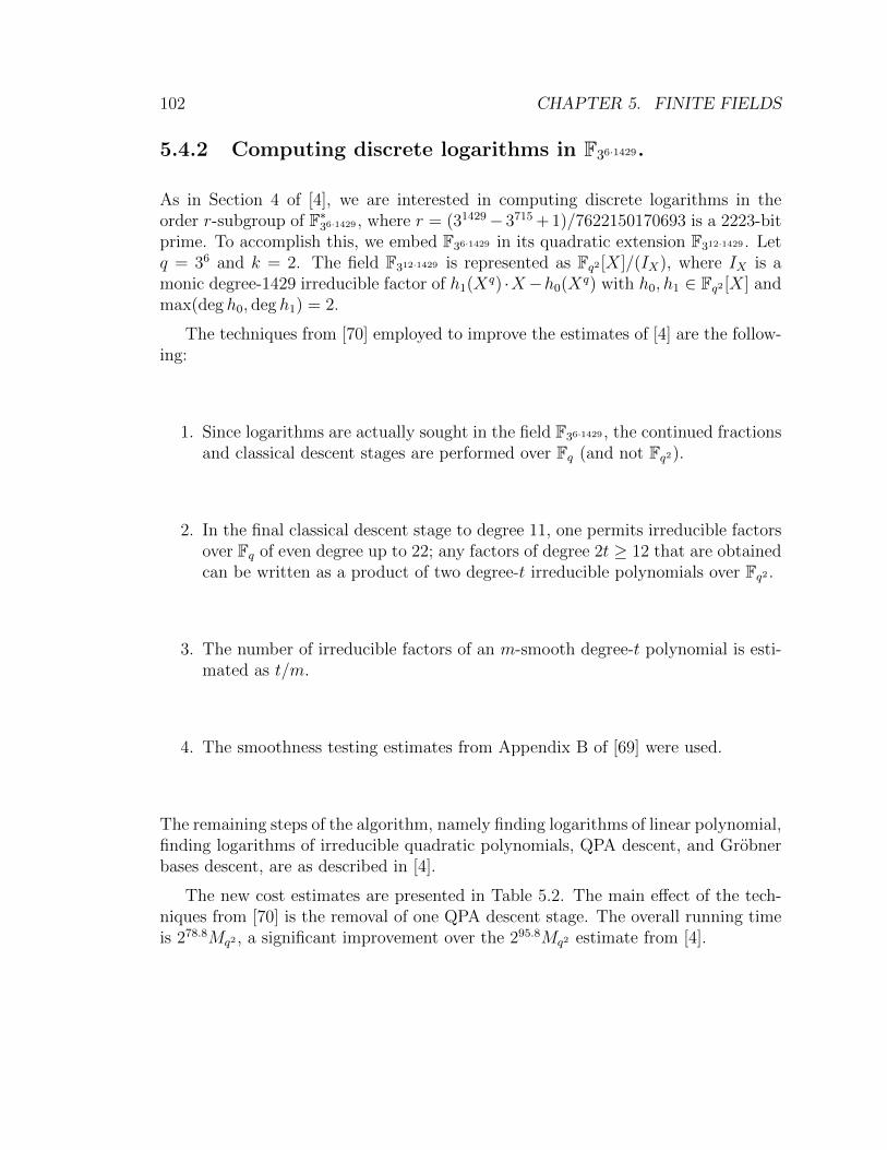
102 CHAPTER 5. FINITE FIELDS
5.4.2 Computing discrete logarithms in F36·1429.
As in Section 4 of [4], we are interested in computing discrete logarithms in theorder r-subgroup of F∗36·1429 , where r = (31429− 3715 + 1)/7622150170693 is a 2223-bitprime. To accomplish this, we embed F36·1429 in its quadratic extension F312·1429 . Letq = 36 and k = 2. The field F312·1429 is represented as Fq2 [X]/(IX), where IX is amonic degree-1429 irreducible factor of h1(Xq) ·X−h0(Xq) with h0, h1 ∈ Fq2 [X] andmax(deg h0, deg h1) = 2.
The techniques from [70] employed to improve the estimates of [4] are the follow-ing:
1. Since logarithms are actually sought in the field F36·1429 , the continued fractionsand classical descent stages are performed over Fq (and not Fq2).
2. In the final classical descent stage to degree 11, one permits irreducible factorsover Fq of even degree up to 22; any factors of degree 2t ≥ 12 that are obtainedcan be written as a product of two degree-t irreducible polynomials over Fq2 .
3. The number of irreducible factors of an m-smooth degree-t polynomial is esti-mated as t/m.
4. The smoothness testing estimates from Appendix B of [69] were used.
The remaining steps of the algorithm, namely finding logarithms of linear polynomial,finding logarithms of irreducible quadratic polynomials, QPA descent, and Grobnerbases descent, are as described in [4].
The new cost estimates are presented in Table 5.2. The main effect of the tech-niques from [70] is the removal of one QPA descent stage. The overall running timeis 278.8Mq2 , a significant improvement over the 295.8Mq2 estimate from [4].
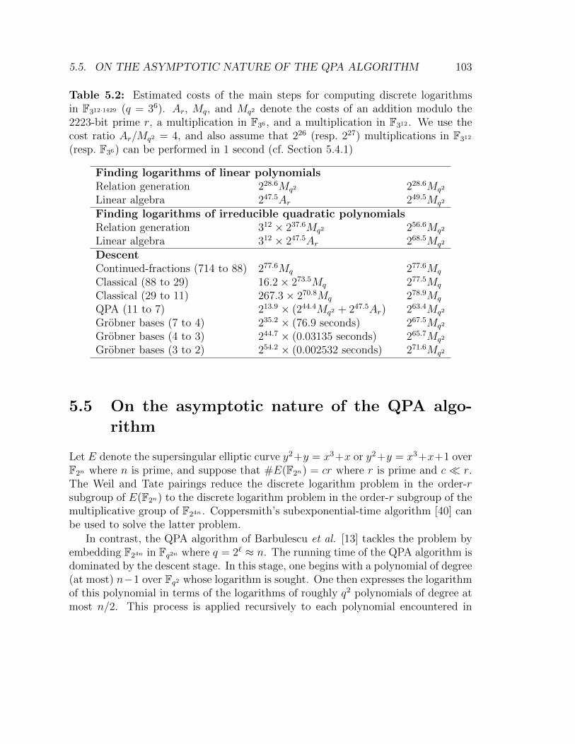
5.5. ON THE ASYMPTOTIC NATURE OF THE QPA ALGORITHM 103
Table 5.2: Estimated costs of the main steps for computing discrete logarithmsin F312·1429 (q = 36). Ar, Mq, and Mq2 denote the costs of an addition modulo the2223-bit prime r, a multiplication in F36 , and a multiplication in F312 . We use thecost ratio Ar/Mq2 = 4, and also assume that 226 (resp. 227) multiplications in F312
(resp. F36) can be performed in 1 second (cf. Section 5.4.1)
Finding logarithms of linear polynomialsRelation generation 228.6Mq2 228.6Mq2
Linear algebra 247.5Ar 249.5Mq2
Finding logarithms of irreducible quadratic polynomialsRelation generation 312 × 237.6Mq2 256.6Mq2
Linear algebra 312 × 247.5Ar 268.5Mq2
DescentContinued-fractions (714 to 88) 277.6Mq 277.6Mq
Classical (88 to 29) 16.2× 273.5Mq 277.5Mq
Classical (29 to 11) 267.3× 270.8Mq 278.9Mq
QPA (11 to 7) 213.9 × (244.4Mq2 + 247.5Ar) 263.4Mq2
Grobner bases (7 to 4) 235.2 × (76.9 seconds) 267.5Mq2
Grobner bases (4 to 3) 244.7 × (0.03135 seconds) 265.7Mq2
Grobner bases (3 to 2) 254.2 × (0.002532 seconds) 271.6Mq2
5.5 On the asymptotic nature of the QPA algo-
rithm
Let E denote the supersingular elliptic curve y2+y = x3+x or y2+y = x3+x+1 overF2n where n is prime, and suppose that #E(F2n) = cr where r is prime and c� r.The Weil and Tate pairings reduce the discrete logarithm problem in the order-rsubgroup of E(F2n) to the discrete logarithm problem in the order-r subgroup of themultiplicative group of F24n . Coppersmith’s subexponential-time algorithm [40] canbe used to solve the latter problem.
In contrast, the QPA algorithm of Barbulescu et al. [13] tackles the problem byembedding F24n in Fq2n where q = 2` ≈ n. The running time of the QPA algorithm isdominated by the descent stage. In this stage, one begins with a polynomial of degree(at most) n−1 over Fq2 whose logarithm is sought. One then expresses the logarithmof this polynomial in terms of the logarithms of roughly q2 polynomials of degree atmost n/2. This process is applied recursively to each polynomial encountered in
104 CHAPTER 5. FINITE FIELDS
the “descent tree”; the logarithm of each such polynomial of degree d is expressedin terms of the logarithms of roughly q2 polynomials of degree at most d/2. Toterminate the recursion, the logarithms of all degree-1 polynomials are obtainedusing a relatively fast method. The number of nodes in the descent tree gives a verycrude lower bound on the running time of the QPA algorithm. Since n ≈ q, thedescent tree has approximately log2 q levels and at least q2 log2 q nodes.
Table 5.3 compares the running time C(q) = exp(1.526(log 24q)1/3(log log 24q)2/3)of Coppersmith’s algorithm for computing discrete logarithms in F24q , and the lowerbound q2 log2 q on the running time of the QPA algorithm for computing discretelogarithms in Fq2n with q ≈ n.
Table 5.3: Comparison of the running time q2 log2 q of the QPA algorithm for com-puting logarithms in Fq2n with q ≈ n, and the running time C(q) of Coppersmith’salgorithm for computing logarithms in F24n
q q2 log2 q C(q)29 2162 293
210 2200 2124
211 2242 2165
212 2288 2219
213 2338 2290
214 2392 2382
215 2450 2501
We see from Table 5.3 that the QPA algorithm is faster than Coppersmith’salgorithm only when n ≈ q = 215. However, such n is too large to be of interest incryptography based on pairings over E(F2n).
As already stated in [13, Section 6.2], to determine the practical efficiency of theQPA algorithm, and therefore the implications of QPA to the security of pairing-based cryptosystems based on E(F2n), it is imperative that the descent stage ofQPA be combined with descent steps from classical algorithms. The asymptoticrunning time of the resulting hybrid algorithm is difficult to determine. Instead, theframework and tools introduced in [2] are used to perform a concrete analysis whichprovides a reasonably accurate picture of the effectiveness of the hybrid algorithm.
5.6. SUMMARY 105
5.6 Summary
In this chapter, we applied the recent techniques for solving the DLP on small-characteristic fields to the cases F36·137 and F36·163 . The implementations were donecompletely in the Magma algebra system and took 918 CPU hours and 1201 CPUhours, respectively.
Next, we realized a concrete analisis of the cost to solve the DLP in the fields F36·509
and F36·1429 using the Joux-Pierrot approach. Both fields were previously proposedas primitives for pairing-based protocols. Finally, we presented estimations for theBarbulescu et al. quasi-polynomial algorithm on different extension fields in orderto verify its feasibility on being applied to fields of cryptographic interest.

106 CHAPTER 5. FINITE FIELDS
6 | Elliptic and Hyperelliptic Curves
In the last two decades, the elliptic curve cryptosystems introduced by Koblitz andMiller [98, 113] have been increasingly employed to instantiate public-key standards[132] and protocols [44, 146]. The main reason for that is their reduced key size,which accommodate fast and lightweight implementations.
In 2011, Galbraith, Lin and Scott (GLS) [61] introduced efficient computableendomorphisms for a large class of elliptic curves defined over Fp2 , where p is a primenumber. Later, Hankerson, Karabina and Menezes [76] analyzed the GLS curvesdefined over characteristic two fields F22n , with prime n. For more details of the GLScurves, see Chapter 3.
Since then, many authors combined the GLS efficient endomorphisms with theGallant-Lambert-Vanstone decomposition method [63] to present high-performancescalar multiplication software implementations over binary [76, 120] and prime [81,103, 29, 50] fields.
The theoretical security of an elliptic curve is given by the complexity of solvingthe discrete logarithm problem (DLP) on its group of points. Given an elliptic curveE defined over a field Fq, a generator point P ∈ E(Fq) of order r and a challengepoint Q ∈ 〈P 〉, the DLP on E consists in computing the integer λ ∈ Zr such thatQ = λP .
Among the classical methods for solving the DLP on E(Fq) we can cite the BabyStep Giant Step [39, Section 19.4] and Pollard Rho [126] algorithms. Both of themrun in time O(
√q). In 1993, Menezes, Okamoto and Vanstone presented a method
[112] that uses the Weil pairing to reduce the DLP on E(Fq) to the same problemon F∗
qk, where k is the smallest positive integer such that r | qk− 1. In binary curves
where k is small, the attack is highly effective, because there exist quasi-polynomialalgorithms for solving the discrete logarithm on small-characteristic finite fields [13].For binary curves, we also have algorithms based on the index-calculus approach [49]which run in time O(
√qω), where ω is a constant related to the linear algebra.
In 2000, Gaudry, Hess and Smart (GHS) [65] applied the ideas in [54, 62] toreduce any instance of the DLP on a binary curve E/F2ln to one on the Jacobian
107
108 CHAPTER 6. ELLIPTIC AND HYPERELLIPTIC CURVES
of a hyperelliptic curve defined over a subfield F2l . Afterwards, Galbraith, Hess andSmart [60] extended the attack by using isogenies. Next, Hess [80] generalized theattack (gGHS) to arbitrary Artin-Schreier extensions.
The analysis of the practical implications of the GHS Weil descent method weremade by Menezes and Qu [108] who demonstrated that the attack is infeasible forelliptic curves over F2n with primes n ∈ [160, . . . , 600] and by Menezes, Teske andWeng [111] who showed that the attack can be applied to curves defined over com-posite extensions of a binary field. Finally, the authors in [76] analyzed the appli-cation of the gGHS attack over GLS binary curves E/F22n and concluded that forn ∈ [80, . . . , 256], the degree-127 extension is the only one that contains vulnerablecurve isogeny classes.
In this work, we wanted to get a practical perspective of the GHS Weil descentattack. In order to achieve this goal, we implemented the attack against a binaryGLS elliptic curve on the Magma computer algebra system. The implementationincluded the construction of vulnerable curves, the search for susceptible isogenouscurves and the adaptation of the Enge-Gaudry algorithm [46] to solve the discretelogarithm problem on the generated hyperelliptic curve.
Moreover, we proposed a mechanism to check for unsafe binary curve parame-ters against the GHS attack. The Magma source code for the algorithms presentedin this document is available at http://computacion.cs.cinvestav.mx/~thomaz/gls.tar.gz. Our program can be easily adapted for any extension field and can beexecuted on single and multi-core architectures.
6.1 Hyperelliptic Curves
Let F2l be a finite field of 2l elements, for some positive integer l, and let F2ln be adegree-n extension field of F2l . A hyperelliptic curve H/F2l of genus g is given bythe following non-singular equation,
H/F2l : y2 + h(x)y = f(x), (6.1)
where f, h ∈ F2l [x], deg(f) = 2g + 1 and deg(h) ≤ g. The set of F2ln-rational pointson H is H(F2ln) = {(x, y) : x, y ∈ F2ln , y
2 + h(x)y = f(x)} ∪ {O}. The opposite of apoint P = (x, y) ∈ H(F2ln) is denoted as P = (x, y + h(x)) and O = O.
The group law is not defined over the curve itself but on the Jacobian of H,denoted by JH(F2l), which is defined in terms of the set of divisors on H. A divisoris a finite formal sum of points on the curve and the set of all divisors on H yieldan abelian group denoted by Div(H). Let ci be an integer, then for each divisor
6.1. HYPERELLIPTIC CURVES 109
D =∑
Pi∈H ci(Pi), deg(D) =∑ci is the degree of D. The set Div0(H) of degree-
zero divisors forms a subgroup of Div(H).
The function field F2ln(H) of H is the set of rational functions on H. For each non-
zero function ϕ ∈ F2ln(H), we can associate a divisor div(ϕ) =∑
Pi∈H νPi(ϕ)(Pi),where νPi(ϕ) is an integer defined as follows:
νPi(ϕ) =
the multiplicity of Pi with respect to ϕ if ϕ has a zero at Pi
the negative of the multiplicity of Piwith respect to ϕ if ϕ has a pole at Pi
0 otherwise.
A non-zero rational function has only finitely many zeroes and poles. In addition,the number of poles equals the number of zeroes (with multiplicity). Therefore,νPi(ϕ) is equal to zero for almost all Pi and div(ϕ) is consequently well defined.
The divisor div(ϕ) is called principal. Given two functions ϕ0 and ϕ1 ∈ F2ln(H),the difference of two principal divisors div(ϕ0) and div(ϕ1) is also a principal divisor,corresponding to the fraction of the two functions. The set P(H) of principal divisorscontains 0 as div(1) and is a subgroup of Div0(H). The Jacobian of the curve H isgiven by the quotient group JH(F2l) = Div0(H)/P(H) and JH(F2l) is the Jacobianover F2l . Note that #JH(F2l) ≈ 2lg.
A consequence of the Riemann-Roch theorem [39, Section 4.4.2] is that everyelement of the Jacobian can be represented by a divisor of the form
D = (P1) + (P2) · · ·+ (Pr)− r(O) (6.2)
where Pi ∈ H for i = 1, . . . , r and r ≤ g. Furthermore, if Pi 6= Pj for all i 6= j, thenD is called a reduced divisor. A reduced divisor can be uniquely represented by apair of polynomials U, V ∈ F2l [x] such that (i) deg(V ) < deg(U) ≤ g; (ii) U is monic;and (iii) U |(V 2 + V h− f).
If U and V are two polynomials that satisfy the above conditions, we denote bydiv(U, V ) the corresponding element of JH(F2l). When U is irreducible in F2l [x] wesay that div(U, V ) is a prime divisor. Let D = div(U, V ) ∈ JH(F2l) and U =
∏Ui,
where each Ui is an irreducible polynomial in F2l [x], and let Vi = V mod Ui. ThenDi = div(Ui, Vi) is a prime divisor and D =
∑Di.
110 CHAPTER 6. ELLIPTIC AND HYPERELLIPTIC CURVES
6.2 The Hyperelliptic Curve Discrete Logarithm
Problem
Let q = 2l and g be the genus of the hyperelliptic curve H/Fq. The discrete logarithmproblem on JH(Fq) is defined as follows: given D1 ∈ JH(Fq) of order r and D2 ∈ 〈D1〉,find λ ∈ Zr such that D2 = λD1.
Besides the Pollard Rho algorithm, whose time complexity is O(√
πqg
2), the meth-
ods proposed in the literature for solving the DLP on H are index-calculus-basedalgorithms:
1. Gaudry in [64] proposed an algorithm whose complexity is O(g3q2 log2 q +g2g!q log2 q). If one considers a fixed genus g, the algorithm executes in time
O(q2+ε). In [65], the algorithm is modified to perform in time O(q2gg+1
+ε). Here,ε is a number less than 1.
2. The Enge-Gaudry algorithm [46] has an expected running time of Lqg [√
2] wheng/ log q →∞. Here, Lx[c] denotes the expression e((c+o(1))
√log x
√log log x).
3. In [66], Gaudry et al. propose a double large prime variation in order to improvethe relation collection phase. For curves with fixed genus g ≥ 3 the algorithm
runs in time O(q2− 2g ).
4. The approach from Sarkar and Singh [137, 138], based on the Nagao’s work[115], avoids the requirement of solving a multi-variate system and combinesa sieving method proposed by Joux and Vitse [90]. They showed that it ispossible to obtain a single relation in about (2g + 3)! trials.
6.3 The Gaudry-Hess-Smart (GHS) Weil descent
attack
Let F2ln be a degree-n extension of F2l and let E be an elliptic curve defined overF2ln given by the equation
E/F2ln : y2 + xy = x3 + ax2 + b a ∈ F2ln , b ∈ F∗2ln . (6.3)
The GHS Weil descent attack [65] consists of the following steps,
1. The Weil descent:

6.3. THE GAUDRY-HESS-SMART (GHS) WEIL DESCENT ATTACK 111
(a) Construct the Weil restriction WE/F2l
of scalars of E, which is an n-dimensional abelian variety over F2l . One can construct this variety asfollows. Let β = {φ1, . . . , φn} be a basis of F2ln viewed as a vector spaceover F2l . Then write a, b, x and y in terms of β,
a =n∑i=1
aiφi, b =n∑i=1
biφi, x =n∑i=1
xiφi and y =n∑i=1
yiφi. (6.4)
Given that β is a linearly independent set, by substituting the equations(6.4) into the equation (6.3) we obtain an n-dimensional abelian varietyA defined over F2l . Moreover, the group law of A is similar to the ellipticcurve E group law.
(b) Intersect A with n − 1 hyperplanes (e.g. x1 = x2 = · · · = xn = x) toobtain a subvariety of A, and then use its linear independence propertyto obtain a curve H over F2l .
2. Reduce the DLP on E(F2ln) to the DLP on JH(F2l).
3. Solve the DLP on JH(F2l).
Let γ ∈ F2ln , σ : F2ln → F2ln be the Frobenius automorphism defined as σ(γ) = γ2l ,γi = σi(γ) for all i ∈ {0, . . . , n− 1} and
m = m(γ) = dim(SpanF2{(1, γ1/2
0 ), . . . , (1, γ1/2n−1)}).
Finally, let us assume that
either n is odd or m(b) = n or TrF2ln
/F2(a) = 0. (6.5)
Then the GHS Weil descent attack constructs an explicit group homomorphismχ : E(F2ln) → JH(F2l), where H is a hyperelliptic curve defined over F2l of genusg = 2m−1 or g = 2m−1 − 1.
6.3.1 The generalized GHS (gGHS) Weil descent attack
In [80] Hess generalized the GHS restrictions (6.5) as follows. Let ℘(x) = x2 +x andF = F2ln(x), ∆ = fF2[σ] + ℘(F ) where f = γ1/x+ γ3 + xγ2 for γ1, γ2, γ3 ∈ F2ln suchthat γ1γ2 6= 0.
Given a polynomial p =∑d
i=0 pixi ∈ F2[x] of degree d we write p(σ)(x) =∑d
i=0 pix2li . For each element γ ∈ F2ln , Ordγ(x) is the unique monic polynomial
112 CHAPTER 6. ELLIPTIC AND HYPERELLIPTIC CURVES
p ∈ F2[x] of least degree such that p(σ)(γ) = 0. Furthermore, we define the m-degree Ordγ1,γ2,γ3 as,
Ordγ1,γ2,γ3 =
{lcm(Ordγ1 ,Ordγ2) if TrF
2ln/F2(γ3) = 0
lcm(Ordγ1 ,Ordγ2 , x+ 1) otherwise.
Then ∆/℘(F ) ∼= F2[x]/Ordγ1,γ2,γ3 and the Frobenius automorphism σ of F withrespect to F2ln extends to a Frobenius automorphism of a function field C = F (℘−1(∆))with respect to F2ln if and only if,
either TrF2ln
/F2(γ3) = 0 or TrF2ln
/F2l
(γ1) 6= 0 or TrF2ln
/F2l
(γ2) 6= 0. (6.6)
In addition, the genus of C is given by
gC = 2m − 2m−deg(Ordγ1 ) − 2m−deg(Ordγ2 ) + 1
and there exists a curve H with genus gC that can be related to an elliptic curveE/F2ln : y2 + xy = x3 + ax2 + b with a = γ3 and b = (γ1γ2)2.
6.3.2 Using isogenies to extend the attacks
Let E and E ′ be two ordinary elliptic curves defined over F2ln and given by theequation (6.3). A rational map Ψ: E → E ′ over F2ln is an element of the ellipticcurve E ′(F2ln(E)). An isogeny Φ: E → E ′ over F2ln is a non-constant rational mapover F2ln and is also a group homomorphism from E(F2ln) to E ′(F2ln). In that case,we say that E and E ′ are isogenous. It is known that E and E ′ are isogenous overF2ln if and only if #E(F2ln) = #E ′(F2ln) [147].
An isogeny Φ: E → E ′ induces a map Φ∗ : F2ln(E ′)→ F2ln(E), called the pullbackof Φ [57], which is necessarily injective,
Φ∗ : F2ln(E ′) → F2ln(E)
θ → θ ◦ Φ.
If x ∈ E ′(F2ln), we can pull back x along Φ, and obtain a divisor
D =∑
P∈Φ−1(x)
νP (Φ)(P ).
The degree δ of Φ is defined by the integer [F2ln(E) : Φ∗(F2ln(E ′))] and we say thatΦ is a δ-isogeny.
The authors in [60] propose to extend the range of vulnerable curves against theGHS attack (and equivalently the gGHS attack) by finding an explicit representationfor an isogeny Φ: E → E ′ and determining if there exists at least one elliptic curveE ′ against which the attack is effective.

6.4. ANALYZING THE GLS ELLIPTIC CURVES 113
6.4 Analyzing the GLS elliptic curves
Let F22n be a degree-2 extension of F2n . Also, let E/F2n be an ordinary elliptic curvegiven by the equation
E/F2n : y2 + xy = x3 + ax2 + b a ∈ F2n , b ∈ F∗2n , (6.7)
with Tr(a) = 1. We know that #E(F2n) = q + 1− t, where t is the trace of E overF2n . It follows that #E(F22n) = (q + 1)2 − t2. Let a′ ∈ F22n such that Tr(a′) = 1.Then we can construct the GLS curve,
E ′/F22n : y2 + xy = x3 + a′x2 + b. (6.8)
Which is isomorphic to E over F24n under the involutive isomorphism τ : E → E ′.The GLS endomorphism can be constructed by applying τ with the Frobenius auto-morphism σ, defined as (x, y) 7→ (x2n , y2n), as follows, ψ = τστ−1.
6.4.1 Applying the GHS Weil descent attack
The theoretical security of a given binary GLS curve E/F22n depends basically onthe complexity of solving the DLP on its group of points E(F22n). As discussed inthe introduction of this chapter, the usual approach is to apply the Pollard Rho
algorithm for elliptic curves, which runs in approximately√
π22n
2operations [126].
However, after the publication of the GHS reduction, it is also necessary to checkwhether the complexities of solving the DLP on JH(F2), JH(F22) or JH(F2n) are lowerthan solving it on E(F22n). If such is the case, the smallest complexity provides usthe real security of the curve E.
Let us assume that the number of isogenous curves E ′ is smaller than the num-ber of vulnerable isogeny classes, then the following steps describe a method fordetermining if a given GLS curve is vulnerable against the extended GHS attack:
1. Setting the environment. Let us have a GLS curve Ea,b/F22n given by the
equation (6.8) but defined with the particular parameters a and b. In thecontext of the GHS attack, the extension field F22n can be seen as a degree-nextension of F22 or a degree-2n extension of F2. For the sake of simplicity, wewill represent the base field as F22 . Nonetheless, the steps must be executedfor both base representations.
114 CHAPTER 6. ELLIPTIC AND HYPERELLIPTIC CURVES
2. Checking the b parameter. We know that (xn + 1)(σ) = x22n + x = 0 ⇔x22n = x. In addition, Ordγ|(xn + 1). Given that the polynomial xn + 1factorizes as (x + 1) · fi · . . . · fs, let d = deg(fi). Then, search a pair ofpolynomials s1 = (x+ 1)j1 · f j2i and s2 = (x+ 1)j3 · f j4i , with positive integers jiand find a representation of b as (γ1γ2)2, such that Ordγi = si(σ) and Ordγ1,γ2,aderive a small associated value gC .
3. Solving the DLP on a hyperelliptic curve. If such minimum pair s1, s2
exists (i), apply the Weil descent on E to construct a hyperelliptic curve H.Check if the complexity of solving the DLP on JH(F22) is smaller than solvingit on E(F22n) (ii). If that is the case, the curve E is vulnerable against theGHS attack. If either (i) or (ii) is false, go to step 4.
4. The extended GHS attack. For each isogenous curve E ′ to E, perform thecheck (steps 2 and 3). If there is no vulnerable elliptic curve E ′ isogenous toE, then the curve E is not vulnerable against the extended GHS attack.
If the number of isogenous curves E ′ is greater than the number of vulnerableisogeny classes, a more efficient method to perform the vulnerability check is to listall vulnerable parameters b and store all of the related group orders #Ea,b(F22n) ina set L. The check consists in verifying whether #Ea,b(F22n) ∈ L [76].
The extension field F22n can also be represented as a degree-2 extension of F2n .However, as analyzed in [76], in this setting the GHS attack generates hyperellipticcurves of genus 2 or 3. Solving the DLP on the Jacobian of these curves is not easierthan solving it on E(F22n) with the Pollard Rho method.
The complexity of solving the DLP on JH(F22) (or JH(F2)) is determined by thegenus of the curve H (see Section 6.2). In the GHS attack context, the genus ofthe constructed hyperelliptic curve H is given by the degree of the minimum pairof polynomials (s1, s2). For each extension degree n, these values are derived fromthe factors of the polynomial xn + 1. For this reason, in characteristic two, we havemany extensions where the genus of H is large and consequently, the GHS attack isineffective for any GLS curve defined over such extension fields.
To illustrate those cases, we present in Table 6.1 the costs of solving the DLPwith the GHS/Enge-Gaudry approach and the Pollard Rho algorithm on binaryGLS curves E/F22n with n ∈ [5, 257]. We chose all the hidden constant factors inthe Enge-Gaudry algorithm complexity to be one, and suppressed all fields whosegenus of the generated curve H is higher than 106. In addition, the effort of findinga vulnerable curve against the GHS attack is not included in the cost for solving theDLP.
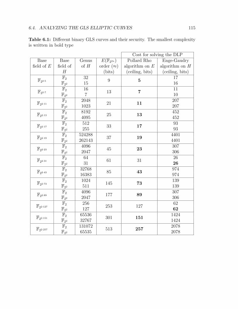
6.4. ANALYZING THE GLS ELLIPTIC CURVES 115
Table 6.1: Different binary GLS curves and their security. The smallest complexityis written in bold type
Cost for solving the DLPBase
field of EBase
field ofH
Genusof H
E(F22n)order (≈)
(bits)
Pollard Rhoalgorithm on E(ceiling, bits)
Enge-Gaudryalgorithm on H(ceiling, bits)
F22·5F2 32
9 517
F22 15 16
F22·7F2 16
13 711
F22 7 10
F22·11F2 2048
21 11207
F22 1023 207
F22·13F2 8192
25 13452
F22 4095 452
F22·17F2 512
33 1793
F22 255 93
F22·19F2 524288
37 194401
F22 262143 4401
F22·23F2 4096
45 23307
F22 2047 306
F22·31F2 64
61 3126
F22 31 26
F22·43F2 32768
85 43974
F22 16383 974
F22·73F2 1024
145 73139
F22 511 139
F22·89F2 4096
177 89307
F22 2047 306
F22·127F2 256
253 12762
F22 127 62
F22·151F2 65536
301 1511424
F22 32767 1424
F22·257F2 131072
513 2572078
F22 65535 2078
116 CHAPTER 6. ELLIPTIC AND HYPERELLIPTIC CURVES
6.4.2 A mechanism for finding vulnerable curves
In this part, we propose a mechanism for performing the step 3 check on the param-eter b of a given GLS curve Ea,b. This mechanism is useful when the number of GHSvulnerable isogeny classes is greater than the number of isogenous curves to Ea,b.Similarly to the previous section, F22n is a degree-n extension field of F22 . However,the method can be easily adapted to any field representation.
Let xn + 1 = (x + 1)f1 · · · fs, where each irreducible polynomial fi ∈ F2[x] hasdegree d and fi 6= fj for i 6= j. Also, let S = {(x + 1)j1f j2i , (x + 1)j3f j4i }ji∈{0,1} bea nonempty finite set where for each pair (s1, s2) ∈ S, deg(s1) ≥ deg(s2). Then letB = {b = (γ1γ2)2 : γ1, γ2 ∈ F∗22n , ∃(s1, s2) ∈ S|s1(σ)(γ1) = 0 ∧ s2(σ)(γ2) = 0}.
Let f, g ∈ F2[x] be two degree-d polynomials. Then we have the following theo-rems:
Theorem 12. (f · g)(σ)(x) = (f(σ) ◦ g(σ))(x) = (g(σ) ◦ f(σ))(x).
Proof. Let q = 22. The expression (f · g)(x) can be written as
(d∑i=0
fixi)(
d∑j=0
gjxj) =
d∑i=0
d∑j=0
figjxi+j.
Then,
(f · g)(σ)(x) =d∑i=0
d∑j=0
figjxqi+j =
d∑i=0
d∑j=0
fi
(gjx
qj)qi
=d∑i=0
fi
d∑j=0
(gjx
qj)qi
=d∑i=0
fi
(d∑j=0
gjxqj
)qi
= (f(σ) ◦ g(σ)) (x).
The proof of the case (f · g)(σ)(x) = (g(σ) ◦ f(σ))(x) is similar.
Theorem 13. f(σ)(x) | (f · g)(σ)(x) over F22n(α1, . . . , αqd) where each αi is a rootof the polynomial f(σ).
Proof. Given that p(σ)(x) has a zero at x = 0 for all polynomial p ∈ F2[x], let αbe a root of f(σ)(x) in its splitting field. Then g(σ)(f(σ)(α)) = g(σ)(0) = 0, i.e.,α is also a root of (f · g)(σ). As a result, f(σ) =
∏(x − αi) divides (f · g)(σ) over
F22n(α1, . . . , αqd).
Theorem 14. ∀γ ∈ F22n, we have that Ordγ(σ)(x) splits on F2.
6.4. ANALYZING THE GLS ELLIPTIC CURVES 117
Proof. From the the previous theorem, we have that for a polynomial p(x) ∈ F2[x],every factor p(x) of p(x) satisfies p(σ)(x)|p(σ)(x) over F22n(α1, . . . , αdeg(p)) where each
αi is a root of p. Then, since Ordγ(x)|xn + 1 we have that Ordγ(σ)(x)|(xq2n + x)over F22n(α1, . . . , αdeg(Ordγ)) where each αi is a root of Ordγ(σ)(x). Consequently,F22n = F22n(α1, . . . , αdeg(Ordγ)) and Ordγ(σ)(x) splits over F2[x].
For a given b ∈ F∗22n , we can determine whether b is in B as follows. For all
(s1, s2) = (∑
j s1,jxj,∑
j s2,jxj) ∈ S, let bi(x) = si(σ)(b1/2x) =
∑j(b
1/2si,j)xqj and
let si(x) = xdeg(si)si(σ)( 1x). Then,
gcd (b1(x), s2(x)) 6= 1 ⇔ ∃γ ∈ F∗22n such that s1(σ)(b1/2γ) = 0 and s2(σ)(1
λ) = 0
⇔ s1(σ)(x) has a zero at γ1 = b1/2γ and
s2(σ)(x) has a zero at γ2 =1
γ
⇔ b = (γ1γ2)2 where s1(σ)(γ1) = 0 and
s2(σ)(γ2) = 0
⇔ b = (γ1γ2)2 ∈ B.
Let us now assume that S contains only the pairs of polynomials (s1, s2) thatconstruct parameters b which are vulnerable against the gGHS attack. Then, for anarbitrary GLS curve E we have that,
Ea,b is vulnerable⇔ ∃(s1, s2) ∈ S such that gcd (b1(x), s2(x)) 6= 1. (6.9)
Complexity analysis. Let s1 = (x + 1)fi be the maximum degree polynomial ofall pairs in S and the complexity of computing the greatest common divisor overelements in S be O((qd+1)
2). Then the complexity for checking a parameter b with
the above mechanism is O(#S(qd+1)2). This complexity is an upper bound because
in practice we see that a gcd in S requires a smaller number of operations.
At last, we summarize the mechanism in Algorithm 24. Note that, for determiningwhether a given b is a vulnerable parameter, the algorithm must be executed in allbase field representations.
118 CHAPTER 6. ELLIPTIC AND HYPERELLIPTIC CURVES
Algorithm 24 A mechanism for verifying the binary curve parameter b
Input: The element b ∈ F∗22n , the polynomial lists b1, s2 obtained from the set S.Output: True if the binary curve defined with a parameter b is vulnerable against
the gGHS attack and False otherwise.
1: aux ← 1, j ← 0
2: while aux = 1 and j < #S do3: j ← j + 14: aux ← gcd(b1[j], s2[j])5: end while
6: if aux 6= 1 then7: return True8: else9: return False
10: end if
6.5 A concrete attack on the GLS curve E/F262
In order to understand the practical implications of the GHS Weil descent algorithmover a binary GLS curve, we implemented a complete attack on a curve defined overthe field F231·2 . Such field was chosen for two reasons: (i) solving the DLP on theJacobian of a hyperelliptic curve obtained by the GHS attack is easier then solvingit on the elliptic curve (see Table 6.1); (ii) the small amount of resources required forsolving the DLP in this curve allowed us to experiment with different approaches tothe problem.
6.5.1 Building a vulnerable curve
Let F22·31 be an extension field of Fq with q = 22·31/n where n ∈ {31, 62}. Then wecan represent the field F262 as follows,
• n = 62, q = 2, F262∼= F2[v]/f(v), with f(v) = v62 + v29 + 1.
• n = 31, q = 22, F22∼= F2[z]/g(z), with g(z) = z2 + z + 1.
a F262∼= F22 [u]/h(u), with h(u) = u31 + u3 + 1
6.5. A CONCRETE ATTACK ON THE GLS CURVE E/F262 119
Also, let E be a binary GLS curve given by the following equation
Ea,b/F262 : y2 + xy = x3 + ax2 + b a ∈ F262 , b ∈ F∗231
Given that the parameter a can be chosen arbitrarily subject to the constraintTrF262/F2(a) = 1, we chose a = z2. The next step was to find a vulnerable parameterb ∈ F∗231 which defines a curve Ea,b that is vulnerable against the gGHS attack.Moreover, to simulate a cryptographic environment, we must have #Ea,b(F262) = c·r,with small c and prime r.
Let x31 + 1 = (x+ 1)f1 · · · f6. We have deg(fi) = 5. Then Tables 6.2 and 6.3 giveus a list of polynomials that generate the vulnerable parameters b = (γ1γ2)2.
Table 6.2: Polynomials Ordγi which generate low-genus hyperelliptic curves for thecase n = 31, q = 22
Ordγ1 Ordγ2 deg(Ordγ1) deg(Ordγ2) m genus E-G algorithmcomplexity
(x+1)fi x+ 1 6 1 6 32 26.46fi x+ 1 5 1 6 31 25.93
Table 6.3: Polynomials Ordγi which generate low-genus hyperelliptic curves for thecase n = 62, q = 2
Ordγ1 Ordγ2 deg(Ordγ1) deg(Ordγ2) m genus E-G algorithmcomplexity
(x+1)2fi x+ 1 7 1 7 64 26.46
At first, we looked for vulnerable parameters b ∈ F∗231 by obtaining the roots ofthe polynomials listed in Tables 6.2 and 6.3. However, for all those b parameters,log2 |r| < 52. For that reason, we considered non-GLS vulnerable parameters b ∈ F∗262for which log2 |r| ≥ 52. As a result, 61 isogeny classes were found. Let L be the setof its group orders. Then, in a 20-core Intel Xeon E5-2658 2.40GHz, we executedfor 70 hours an extensive search through all b ∈ F∗231 checking if #Ea,b(F262) ∈ L.However, no isogenous curves were found and the extended GHS attack could notbe carried out.
Next, under the setting (n = 31, q = 22), we chose the vulnerable parameterb = u24 + u17 + u16 + u12 + u5 + u4 + u3 + u + 1, which allowed us to construct agroup with order #Ea,b(F262) = 4611686014201959530. The size of our subgroup ofinterest is of about 51 bits. In theory, solving the DLP on this subgroup through the

120 CHAPTER 6. ELLIPTIC AND HYPERELLIPTIC CURVES
Pollard Rho method would take about 226 steps, which is the same cost as solvingthe DLP with the GHS/Enge-Gaudry approach.
Finally, we created an order-r generator point P ∈ Ea,b(F262) with the MagmaRandom function:
P (x, y) =(u30 + z2u28 + zu27 + u26 + zu25 + zu24 + u23 + z2u20 + u18 + zu17
+ zu16 + u15 + u12 + z2u10 + zu9 + z2u8 + u7 + zu6 + u4 + u2
+ z2u+ z,
zu30 + z2u29 + z2u26 + z2u25 + zu24 + u23 + z2u22 + z2u21 + zu20
+ u19 + zu18 + u17 + u15 + zu14 + zu13 + z2u12 + z2u10 + zu9 + u8
+ zu7 + u6 + u2 + zu).
The challenge Q was generated with the same function:
Q(x, y) =(u29 + z2u28 + u27 + u26 + z2u25 + zu24 + u23 + zu22 + z2u20 + z2u17
+ z2u16 + zu12 + u11 + zu10 + z2u9 + z2u8 + zu7 + zu6 + z2u5 + zu4+
z2u2 + u+ z2,
u30 + u29 + z2u28 + u27 + zu26 + z2u24 + zu22 + u21 + z2u20 + z2u19
+ zu18 + zu17 + zu15 + u14 + zu12 + z2u11 + u10 + z2u9 + u6 + u5
+ z2u3 + z2u2 + z2u+ z).
Then we constructed the following genus-32 hyperelliptic curve with the Weil descentmethod1:
H(F22) : y2 + (z2x32 + x16 + z2x8 + z2x2 + x)y =
x65 + x64 + z2x33 + zx32 + x17 + z2x16 + x8 + x5 + x4 + z2x3 + zx2 + zx.
The points P,Q were mapped to the JH(F22), which generated the divisors DP andDQ.
6.5.2 Adapting the Enge-Gaudry Algorithm
To solve the DLP on JH(Fq), with q = 22 and genus g = 32, we adapted theEnge-Gaudry algorithm by restricting the factor base size in order to balance the
1In this step, we used the function WeilDescent from Magma..
6.5. A CONCRETE ATTACK ON THE GLS CURVE E/F262 121
relation collection and the linear algebra phases. According to [46], we can balancethe two phases by selecting the factor base degree as m = dlogq Lqg [%]e where % =√
12
+ 14ϑ−√
14ϑ
for some positive integer ϑ which complies with (i) g ≥ ϑ log q and
(ii) q ≤ Lqg [1√ϑ]. Similarly to the Section 6.4, we chose the constant factors of the
algorithm complexity to be one. For all values of ϑ that satisfy the restrictions (i)and (ii), we have m = [4, 6].
However, in practice, we constructed the factor base dynamically. At first, weinitialized our base F as an empty set and imposed a restriction so that F cancontain polynomials up to degree m. Next, for each valid relation in the Enge-Gaudry algorithm, that is, when the polynomial U of a divisor D = div(U, V ) isd-smooth, we included in F all irreducible factors of U which were not in F . Finally,when the number of relations were equal to the number of factors in F , we concludedthe relations collection phase.
Experimentally, we saw that, at the end of the relations collection phase, just aportion of the irreducible polynomials of degree less or equal than m were includedin F . For that reason, in order to have approximately the same factor base size asif we had constructed a factor base with all irreducible polynomials of degree up to6, we chose m = 7. The algorithm was executed within the Magma v2.20-2 system,in one core of a Intel Core i7-4700MQ 2.40GHz machine. The timings of each phaseare presented below.
Table 6.4: Timings for the adapted Enge-Gaudry algorithm
Random walk initialization 3.00 sRelations collection 284.52 s
Linear Algebra (Lanczos) 0.11 s
At the end of the relation collection phase, our factor basis had 1458 elements,which is 44.12% of the total number of irreducible polynomials of degree 7 andbelow. Although the algorithm phases were not balanced as expected, solving thelinear algebra system was trivial, and we considered our degree selection satisfactory.Finally, the computed discrete logarithm is given as λ = 2344450470259921.
An analysis of the algorithm balance: the genus-32 case
In order to verify the theoretical balance of [46] in the context of the dynamic factorbase construction, we executed the algorithm with different factor base degree limits.The results are presented in Table 6.5.
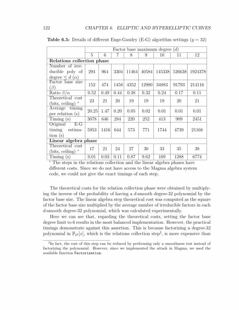
122 CHAPTER 6. ELLIPTIC AND HYPERELLIPTIC CURVES
Table 6.5: Details of different Enge-Gaudry (E-G) algorithm settings (g = 32)
Factor base maximum degree (d)5 6 7 8 9 10 11 12
Relations collection phaseNumber of irre-ducible poly ofdegree ≤ d (α)
294 964 3304 11464 40584 145338 526638 1924378
Factor base size(β)
152 474 1458 4352 12980 34883 91793 214116
Ratio β/α 0.52 0.49 0.44 0.38 0.32 0.24 0.17 0.11Theoretical cost(bits, ceiling) ∗
23 21 20 19 19 19 20 21
Average timingper relation (s)
20.25 1.47 0.20 0.05 0.02 0.01 0.01 0.01
Timing (s) 3078 646 284 220 252 413 909 2451Original E-Gtiming estima-tion (s)
5953 1416 644 573 771 1744 4739 21168
Linear algebra phaseTheoretical cost(bits, ceiling) ∗
17 21 24 27 30 33 35 38
Timing (s) 0.01 0.03 0.11 0.87 9.62 169 1288 6774∗ The steps in the relations collection and the linear algebra phases havedifferent costs. Since we do not have access to the Magma algebra systemcode, we could not give the exact timings of each step.
The theoretical costs for the relation collection phase were obtained by multiply-ing the inverse of the probability of having a d-smooth degree-32 polynomial by thefactor base size. The linear algebra step theoretical cost was computed as the squareof the factor base size multiplied by the average number of irreducible factors in eachd-smooth degree-32 polynomial, which was calculated experimentally.
Here we can see that, regarding the theoretical costs, setting the factor basedegree limit to 6 results in the most balanced implementation. However, the practicaltimings demonstrate against this assertion. This is because factorizing a degree-32polynomial in F22 [x], which is the relations collection step2, is more expensive than
2In fact, the cost of this step can be reduced by performing only a smoothness test instead offactorizing the polynomial. However, since we implemented the attack in Magma, we used theavailable function Factorization.
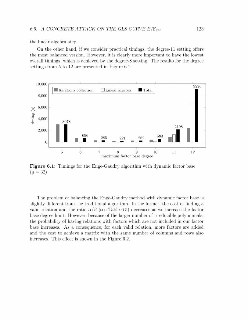
6.5. A CONCRETE ATTACK ON THE GLS CURVE E/F262 123
the linear algebra step.
On the other hand, if we consider practical timings, the degree-11 setting offersthe most balanced version. However, it is clearly more important to have the lowestoverall timings, which is achieved by the degree-8 setting. The results for the degreesettings from 5 to 12 are presented in Figure 6.1.
5 6 7 8 9 10 11 12
0
2,000
4,000
6,000
8,000
10,000
3078
696285 221 262 583
2198
9226
maximum factor base degree
timing(s)
Relations collection Linear algebra Total
Figure 6.1: Timings for the Enge-Gaudry algorithm with dynamic factor base(g = 32)
The problem of balancing the Enge-Gaudry method with dynamic factor base isslightly different from the traditional algorithm. In the former, the cost of finding avalid relation and the ratio α/β (see Table 6.5) decreases as we increase the factorbase degree limit. However, because of the larger number of irreducible polynomials,the probability of having relations with factors which are not included in our factorbase increases. As a consequence, for each valid relation, more factors are addedand the cost to achieve a matrix with the same number of columns and rows alsoincreases. This effect is shown in the Figure 6.2.
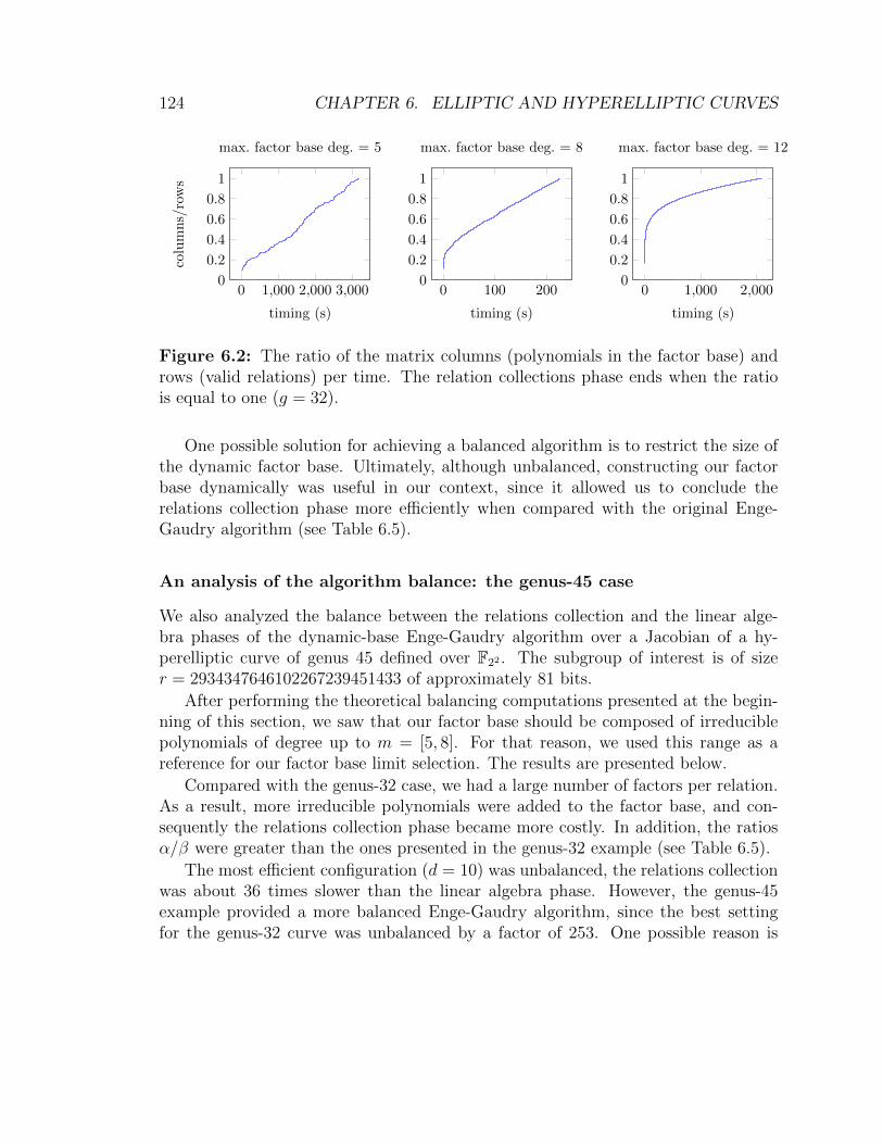
124 CHAPTER 6. ELLIPTIC AND HYPERELLIPTIC CURVES
0 1,000 2,000 3,0000
0.2
0.4
0.6
0.8
1
timing (s)
columns/rows
max. factor base deg. = 5
0 100 2000
0.2
0.4
0.6
0.8
1
timing (s)
max. factor base deg. = 8
0 1,000 2,0000
0.2
0.4
0.6
0.8
1
timing (s)
max. factor base deg. = 12
Figure 6.2: The ratio of the matrix columns (polynomials in the factor base) androws (valid relations) per time. The relation collections phase ends when the ratiois equal to one (g = 32).
One possible solution for achieving a balanced algorithm is to restrict the size ofthe dynamic factor base. Ultimately, although unbalanced, constructing our factorbase dynamically was useful in our context, since it allowed us to conclude therelations collection phase more efficiently when compared with the original Enge-Gaudry algorithm (see Table 6.5).
An analysis of the algorithm balance: the genus-45 case
We also analyzed the balance between the relations collection and the linear alge-bra phases of the dynamic-base Enge-Gaudry algorithm over a Jacobian of a hy-perelliptic curve of genus 45 defined over F22 . The subgroup of interest is of sizer = 2934347646102267239451433 of approximately 81 bits.
After performing the theoretical balancing computations presented at the begin-ning of this section, we saw that our factor base should be composed of irreduciblepolynomials of degree up to m = [5, 8]. For that reason, we used this range as areference for our factor base limit selection. The results are presented below.
Compared with the genus-32 case, we had a large number of factors per relation.As a result, more irreducible polynomials were added to the factor base, and con-sequently the relations collection phase became more costly. In addition, the ratiosα/β were greater than the ones presented in the genus-32 example (see Table 6.5).
The most efficient configuration (d = 10) was unbalanced, the relations collectionwas about 36 times slower than the linear algebra phase. However, the genus-45example provided a more balanced Enge-Gaudry algorithm, since the best settingfor the genus-32 curve was unbalanced by a factor of 253. One possible reason is

6.5. A CONCRETE ATTACK ON THE GLS CURVE E/F262 125
Table 6.6: Details of different Enge-Gaudry algorithm settings (g = 45)
Factor base maximum degree (d)7 8 9 10 11 12 13
Relations collection phaseNumber of irre-ducible poly ofdegree ≤ d (α)
3304 11464 40584 145338 526638 1924378 7086598
Factor base size(β)
1626 5227 16808 52366 158226 460240 1268615
Ratio β/α 0.49 0.46 0.41 0.36 0.30 0.24 0.18Theoretical cost(bits, ceiling) ∗
27 26 25 25 25 25 26
Average timingper relation (s)
29.45 4.60 1.05 0.29 0.12 0.07 0.09
Timing (s) 47895 24067 17621 15204 18909 32630 107902Original E-Gtiming estima-tion (s)
97319 52780 42532 42148 62670 136631 602361
Linear algebra phaseTheoretical cost(bits, ceiling) ∗
25 28 31 34 37 40 43
Timing (s) 0.62 3.79 39 421 4804 48661 417920∗ The steps in the relations collection and the linear algebra phases havedifferent costs. Since we do not have access to the Magma algebra systemcode, we could not give the exact timings of each step.
that, here, each linear algebra steps computed over operands of about 81 bits, whichare 30 bits longer than the operands processed in the genus-32 linear algebra steps.
We expect that, for curves with larger genus, with respectively larger subgroups,a fully balanced configuration can be found. The results for each setting in the45-genus example is shown in Figure 6.3.
In Figure 6.4, we show the progression of the ratio
number of valid relations
factor base size
during the relations collection phase. Similarly to the genus-32 case, for biggerd values, the rate of the factor base growth stalled the progress of the relationscollection algorithm. Again, one potential solution to this issue is to impose limitson the factor base size.
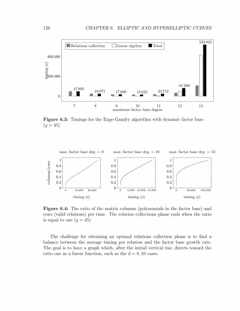
126 CHAPTER 6. ELLIPTIC AND HYPERELLIPTIC CURVES
7 8 9 10 11 12 13
0
200,000
400,000
47 89524 071 17 660 15 625 23 712
81 290
525 822
maximum factor base degree
timing(s)
Relations collection Linear algebra Total
Figure 6.3: Timings for the Enge-Gaudry algorithm with dynamic factor base(g = 45)
0 10,000 20,0000
0.2
0.4
0.6
0.8
1
timing (s)
columns/rows
max. factor base deg. = 8
0 5,000 10,000 15,0000
0.2
0.4
0.6
0.8
1
timing (s)
max. factor base deg. = 10
0 50,000 100,0000
0.2
0.4
0.6
0.8
1
timing (s)
max. factor base deg. = 13
Figure 6.4: The ratio of the matrix columns (polynomials in the factor base) androws (valid relations) per time. The relation collections phase ends when the ratiois equal to one (g = 45)
The challenge for obtaining an optimal relations collection phase is to find abalance between the average timing per relation and the factor base growth rate.The goal is to have a graph which, after the initial vertical rise, directs toward theratio one as a linear function, such as the d = 8, 10 cases.
6.6. SUMMARY 127
6.5.3 The Pollard Rho method
In order to verify the correspondence between the theoretical complexities and thepractical results, we implemented the Pollard rho method which, for GLS curvesE/F22·31 , requires about 29.65 times the amount of work to solve the DLP with theGHS/Enge-Gaudry approach (see Table 6.1).
Our Pollard rho random walk implementation was based on the r-adding walk(with r = 100) method proposed in [149] and on the Floyd’s cycle-finding technique.The algorithm was also implemented on Magma and executed in eight cores of aIntel Xeon E5-2650 2.60GHz machine.
After computing 68880848 points, we found the discrete logarithm in 63.18 CPUhours. Each step of the algorithm, which includes two modular integer addition andone point addition, took about 0.026 seconds. Comparing the practical experimentsof the Pollard rho and the GHS/Enge-Gaudry algorithms, we have that the latteris about 6329.23 times faster. Note that, both implementations could be possiblyimproved by implementing them in C and exploiting the computing resources of ourparticular architetcure.
6.6 Summary
Here, we presented an implementation of the GHS attack against a binary GLS curvedefined over F22·31 . The DLP was solved in the Jacobian of a genus-32 hyperellipticcurve over F22 with a modified version of the Enge-Gaudry algorithm. In this version,we used a dynamic factor base in the relations collection phase. As a result, thisphase proved to be more than twice as fast as the factor base proposed in the originalalgorithm.
Moreover, we realized experiments to understand the dynamic factor base mech-anism with different configurations. In order to strengthen our conclusion, we alsoprovided experiments in the Jacobian of a genus-45 binary hyperelliptic curve.

128 CHAPTER 6. ELLIPTIC AND HYPERELLIPTIC CURVES

Part III
Conclusion

7 | Final Discussions
In the subsequent sections we present a general analysis of the work presented inthis thesis. We start by enumerating our main contributions and then examinethe impact of them in the development of cryptography primitives constructed oversmall-characteristic fields. Finally, we consider the problems and challenges left forfuture research and the open possibilities for investigation in the technological andalgorithmic areas.
7.1 Contributions
In the following paragraphs, we concisely specify our contributions in the area ofhigh-speed elliptic curve cryptography,
• A new system of projective coordinates, denominated lambda coordinates, whichprovided state-of-the-art formulas for computing the point arithmetic in binaryelliptic curves. In addition, its form (x, λ = x + y
x), is particularly appropri-
ate for scalar multiplication methods based on the point halving operation,since it bypasses the point coordinates transformation overhead imposed bythis operation.
• Design of efficient base (Fq) and quadratic (Fq2) field arithmetic. More pre-cisely, the implementation of fast arithmetic for the case q = 2127 aimed forhigh-end desktops. This implementation exploits the 128-bit SSE/AVX vectorset of instructions and the 64-bit carry-less multiplier, both technologies whichare ubiquitous on current desktop platforms. Our efficient arithmetic, alongwith the lambda coordinate system formulas, supported the speed-record soft-ware implementation of a 128-bit secure scalar multiplication in a binary GLScurve.
131
132 CHAPTER 7. FINAL DISCUSSIONS
• A novel right-to-left halve-and-add Montgomery ladder algorithm. For thefirst time, the point halving operation could be applied efficiently in a scalarmultiplication algorithm based on the Montgomery ladder. In addition, thealgorithm precomputes the points to be added throughout the main iteration.As a consequence, a major speed-up is expected in the fixed-point scenario.
• The first timing-resistant scalar multiplication algorithm designed for four-core platforms. To achieve this, we combined the double-and-add left-to-right(without precomputation) and the halve-and-add right-to-left (with precom-putation) Montgomery ladder point multiplication approaches with the endo-morphism provided by the GLS binary curves. As a result, we improved by50% the one-core 128-bit secure Montgomery double-and-add algorithm imple-mentation.
• A regular τ -adic recoding based on the work in [91]. This method was anecessary step for the implementation of the first timing-attack resistant scalarmultiplication in Koblitz curves, which surpassed by 26% the fastest protectedMontgomery ladder point multiplication implementation on Koblitz curves [25].
• The construction of a new family of Koblitz curves defined over a prime ex-tension of the field F4. The arithmetic in quadratic fields is well-suited forimplementation on concurrent computing architectures, such as the currentdesktops and some mobile devices. As a result, we achieved a speed recordin protected 128-bit software scalar multiplication implementation on Koblitzcurves.
• Finally, we developed base arithmetic fully based on redundant trinomials [45].Our scalar multiplication in Koblitz curves over F4 was implemented using thetrinomial g(x) = x192 +x19 +1, which was carefully selected in order to provideefficient timings for the main base arithmetic operations: multiplication andsquaring.
Next, we list our contributions in the area of the discrete logarithm problem,
• A concrete analysis of the impact of the recent discrete logarithm problemadvances [86, 68, 13, 70, 89] on the pairing-friendly fields F36·509 and F36·1429 .Our study was important to understand the computing costs for solving theDLP on fields of cryptographic importance. Also, it assisted the community indeciding whether those fields are secure to be employed in practical protocols.
7.1. CONTRIBUTIONS 133
• The practical application of the new methods for solving the DLP over small-characteristic fields to the cases F36·137 and F36·163 . The field F36·163 was previ-ously considered for implementing pairing-based protocols [26, 59]. Our com-putations were temporarily established as a record in breaking cryptographic-relevant fields.
• An implementation of the GHS attack against a GLS binary elliptic curvedefined over F22·31 with the Magma algebraic system. The implementationshowed us that, in practice, the GHS attack is more efficient than the PollardRho approach, even though both have approximately the same theoretical cost.
• The analysis of the cost of the Enge-Gaudry algorithm [46] for solving the dis-crete logarithm problem with a dynamic factor base. In this work, we realizedexperiments to determine the best factor base configuration in order to balancethe relation collection and the linear algebra phases. Moreover, we showed howthis optimal setting differs from the theoretical balance, which are based onasymptotic cost estimates.
7.1.1 Publications
The work presented in this document were published in the following papers,
• T. Oliveira, J. Lopez, D. F. Aranha and F. Rodrıguez-Henrıquez. LambdaCoordinates for Binary Elliptic Curves. In Cryptographic Hardware and Em-bedded System - CHES 2013, volume 8086 of LNCS, pages 311 - 330. SpringerBerlin Heidelberg, 2013.
• G. Adj, A. Menezes, T. Oliveira and F. Rodrıguez-Henrıquez. Weakness ofF36·509 for Discrete Logarithm Cryptography. In Pairing-Based Cryptography- Pairing 2013, volume 8365 of LNCS, pages 20 - 44. Springer InternationalPublishing, 2014.
• T. Oliveira, J. Lopez, D. F. Aranha and F. Rodrıguez-Henrıquez. Two isthe fastest prime: lambda coordinates for binary elliptic curves. Journal ofCryptographic Engineering, 4(1):3 - 17, 2014.
• T. Oliveira, J. Lopez, D. F. Aranha and F. Rodrıguez-Henrıquez. Fast PointMultiplication Algorithms for Binary Elliptic Curves with and without Pre-computation. In Selected Areas in Cryptography - SAC 2014, volume 8781 ofLNCS, pages 324 - 344. Springer International Publishing, 2014.
134 CHAPTER 7. FINAL DISCUSSIONS
• G. Adj, A. Menezes, T. Oliveira and F. Rodrıguez-Henrıquez. Computing Dis-crete Logarithms in F36·137 and F36·163 Using Magma. In International Workshopon the Arithmetic of Finite Fields - WAIFI 2014, volume 9061 of LNCS, pages3 - 22. Springer International Publishing, 2014.
• G. Adj, A. Menezes, T. Oliveira and F. Rodrıguez-Henrıquez. Weakness ofF36·1429 and F24·3041 for discrete logarithm cryptography. Finite Fields and TheirApplications, 32:148 - 170, 2015.
• T. Oliveira and J. Chi. Attacking a Binary GLS Elliptic Curve with Magma.In Progress in Cryptology - LATINCRYPT 2015, volume 9230 of LNCS, pages308 - 326. Springer International Publishing, 2015.
7.2 Advances
Recently, a number of new approaches for solving the discrete logarithm problem inelliptic curves (ECDLP) were proposed. Those advances, concisely discussed in [58],brought doubt and mistrust to the practical use of binary curves in the academiccommunity [135]. However, the same authors in [58] concluded their survey with thefollowing statement,
The current situation, not at all definitive, is that there is no consensuswhether there is a subexponential algorithm for ECDLP in characteristic2.
Considering this current scenario, our work proposed, through new technologicaland algorithmic ideas, alternative methods to compute, in software, efficient andsecure scalar multiplications on binary curves. Our result showed that the binarycurves are highly competitive with the mainstream approaches on prime curves.
In the discrete logarithm problem (DLP) area, our theoretical analysis of theimpact of the recently proposed algorithms to solve the DLP on small-characteristicfields in pairing-based fields helped to clarify the range of fields which are suitable forthe secure instantitation of pairing-based protocols. Moreover, our implementationof the attacks against fields that were previously proposed in the literature depictedthe potential of the recent approaches.
Finally, our work on the DLP on binary GLS curves provided a better compre-hension of the practical implications of the gGHS attack on this novel family ofcurves. In addition, we presented, for the first time, a concrete analysis of the effectof the dynamic factor base to the Enge-Gaudry algorithm for solving the DLP on ahyperelliptic curve.
7.3. FUTURE WORK 135
7.3 Future work
7.3.1 Open questions
In this section, we list the open problems related to our work. The problems are notpresented in any order of significance, but grouped by the two main subjects of ourthesis.
Are there more efficient approaches to compute the inversion operationin binary fields? After the publication, in 1988, of the Itoh-Tsujii algorithm [84]for inversion in binary fields1, there wasn’t any major advances to improve the effi-ciency of this operation. The continuous decrease of the carry-less multiplier latencyand throughput emphasizes even more the high cost of the inversion function. Forinstance, in the Haswell architecture, the relation between the inversion and multi-plication costs (in clock cycles) is more than thirty (see Section 4.2.5).
An efficient inversion operation would open more possibilities in the implemen-tation of the scalar multiplication algorithm. For example, one could choose torepresent the points with affine coordinates, whose arithmetic are based on inver-sions and, consequently, reduce the required amount of memory throughout the mainiteration of the algorithm.
Is the Karatsuba method faster than the schoolbook algorithm? Asymp-totically, the Karatsuba technique computational complexity of O(nlog23) is betterthan the O(n2) complexity of the schoolbook approach. However, in practice, thecost of pre- and post-processing the operands is higher in the Karatsuba algorithm.In addition, the cost of multiplying two 64-bit operands is approaching the cost ofthe basic logical operations, which are used in the peripheral phases of the Karatsubamethod. The evolution of these instructions costs is shown in Table 7.1.
As a result, when multiplying polynomials stored in a few words (i.e. two orthree), the schoolbook algorithm may be faster. Let us analyze the two-word case.For the Karatsuba method we need three multiplications and twelve logical instruc-tions, while the schoolbook algorithm requires four multiplications and five logicalinstructions. If we have a scenario where one 64-bit carry-less multiplication costsless than seven logical operations, then the schoolbook method is more efficient.
1As the title of the article suggests, the method was devised for finite fields elements representedby a normal basis, where the squaring operation is computed by low-cost circular shifts. In thecase of the polynomial representation, it is too much expensive to compute the algorithm throughmultiple squarings. As a consequence, precomputed tables are required (see Section 3.1.3).
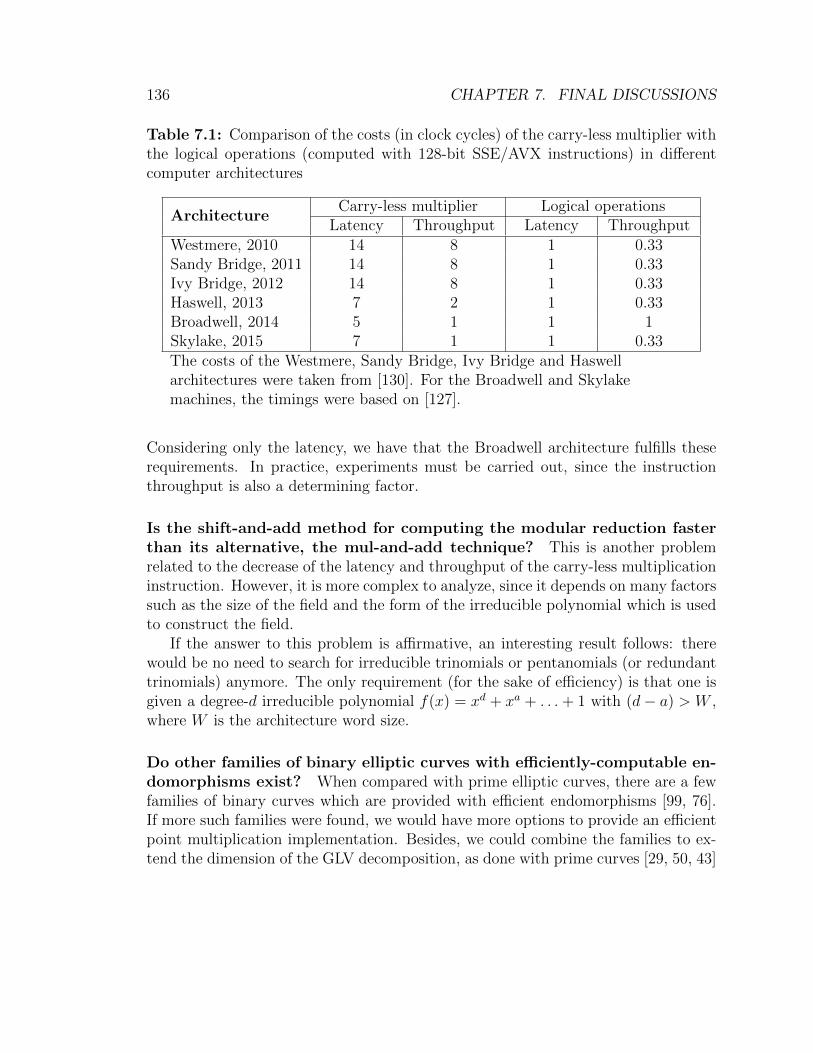
136 CHAPTER 7. FINAL DISCUSSIONS
Table 7.1: Comparison of the costs (in clock cycles) of the carry-less multiplier withthe logical operations (computed with 128-bit SSE/AVX instructions) in differentcomputer architectures
ArchitectureCarry-less multiplier Logical operations
Latency Throughput Latency ThroughputWestmere, 2010 14 8 1 0.33Sandy Bridge, 2011 14 8 1 0.33Ivy Bridge, 2012 14 8 1 0.33Haswell, 2013 7 2 1 0.33Broadwell, 2014 5 1 1 1Skylake, 2015 7 1 1 0.33The costs of the Westmere, Sandy Bridge, Ivy Bridge and Haswellarchitectures were taken from [130]. For the Broadwell and Skylakemachines, the timings were based on [127].
Considering only the latency, we have that the Broadwell architecture fulfills theserequirements. In practice, experiments must be carried out, since the instructionthroughput is also a determining factor.
Is the shift-and-add method for computing the modular reduction fasterthan its alternative, the mul-and-add technique? This is another problemrelated to the decrease of the latency and throughput of the carry-less multiplicationinstruction. However, it is more complex to analyze, since it depends on many factorssuch as the size of the field and the form of the irreducible polynomial which is usedto construct the field.
If the answer to this problem is affirmative, an interesting result follows: therewould be no need to search for irreducible trinomials or pentanomials (or redundanttrinomials) anymore. The only requirement (for the sake of efficiency) is that one isgiven a degree-d irreducible polynomial f(x) = xd + xa + . . .+ 1 with (d− a) > W ,where W is the architecture word size.
Do other families of binary elliptic curves with efficiently-computable en-domorphisms exist? When compared with prime elliptic curves, there are a fewfamilies of binary curves which are provided with efficient endomorphisms [99, 76].If more such families were found, we would have more options to provide an efficientpoint multiplication implementation. Besides, we could combine the families to ex-tend the dimension of the GLV decomposition, as done with prime curves [29, 50, 43]

7.3. FUTURE WORK 137
and, consequently, accelerate the scalar multiplication computation.
Is it possible to compute the point halving operation in projective coor-dinates? Computing a timing-resistant right-to-left halve-and-add scalar multipli-cation is not feasible in practice. This is because the right-to-left approach impliesa higher overhead in order to protect the point multiplication. More precisely, wemust apply the linear pass function twice on the accumulator points (see Sections3.3 and 4.2.4). When the NAF-width w value is big (e.g. four or five), this overheadbecomes too high.
However, to perform the left-to-right approach efficiently, we need that the ac-cumulator point be represented in projective coordinates throughout the main pointmultiplication loop. If we could devise a method to perform the point halving in pro-jective coordinates which was faster than the projective point doubling operation, wecould improve the efficiency of the protected scalar multiplication in binary curves.
Can we apply the GLV decomposition method with the Montgomery lad-der algorithm? In Section 3.4, we presented a method combining the GLV ap-proach with the Montgomery ladder in order to compute the scalar multiplication inthe multi-core scenario. However, for a one-core architecture, it is not known howto maintain the Montgomery ladder point difference together with the applicationsof a non-trivial endomorphism.
If the same speed-ups obtained in the GLV approach were achieved in the Mont-gomery ladder algorithm, we would have the fastest timing-resistant scalar multipli-cation approach.
Is it faster to solve the DLP over small-characteristic fields with FPGAs?It would be useful to analyze the performance of FPGAs to perform the first de-scent phases (i.e. continuous-fraction and classical) of the DLP algorithms. Thosephases consist of multiple instances of simple functions, such as the polynomial mul-tiplication and smoothness testing, which are fully independent. As a result, theimplementation of these algorithms in FPGAs could be faster than executing themin desktop machines that are embedded with just four to sixteen cores.
Can we use GPUs to accelerate the relations collection phase of theEnge-Gaudry algorithm? The relations collection phase is one of the most cru-cial steps of the Enge-Gaudry method for solving the DLP in hyperelliptic curves.If we improve the efficiency for collecting a relation, we could reduce the factor base

138 CHAPTER 7. FINAL DISCUSSIONS
degree and, consequently, would have a smaller set of equations to be solved in thesubsequent linear algebra step.
The challenge is to devise an implementation for adding divisors which is suitablefor efficient implementation in many GPU threads. Also, this implementation mustrequire a minimum amount of memory, in order to extend the GPU parallelism.
Is there a polynomial-time algorithm to solve the DLP over small-char-acteristic fields? After the recent outstanding advances in solving the DLP oversmall-characteristic fields, which included a quasi-polynomial algorithm [13], the ex-pectations for finding a polynomial-time approach in the near future are high. How-ever, one questions whether another framework will be required for such an achieve-ment. In practice, we must devise an efficient descent method which outpaces theone based on the complex Grobner basis algorithm for solving bilinear equations.
7.3.2 Further possibilities
Next, we present different subjects that could complement and advance the workdeveloped in this thesis.
Implementation of the GLS and Koblitz curves scalar multiplication indifferent architectures and scenarios. In this thesis, we presented point multi-plication implementations focused on high-end desktop architectures. However, it isworthwhile to analyze the efficiency of those curves in constrained platforms, whereresources such as memory and power are scarce, the instruction set is simpler andthe register size is smaller. On the other hand, architectures that provides a higherlevel of parallelism, such as GPUs, could also be explored.
In addition, the fixed-point setting should also be analyzed, since it is part ofelliptic curve-based digital signatures protocols [132].
Instruction-level parallelism in the point multiplication implementations.The opportunities for applying the 256-bit AVX instruction set and its future 512-bit extension (AVX-512) to scalar multiplication implementations could be studied.The larger 256-bit registers could be used to generate an efficient one-step shift-and-add modular reduction. Also, the same techniques used to implement a 128-bitbase arithmetic could be applied to higher security levels by using larger vectorizedregisters.
7.3. FUTURE WORK 139
Alternative methods to avoid side-channel attacks based on the CPUcache. As we increase the NAF w-width, we also increase the pre- and post-computation overhead. At the same time, we save point additions in the scalarmultiplication main loop. The bound for selecting the value of w lies on the balancebetween these two phases2. For timing attack-resistant implementations, the w valuealso determines the not-negligible linear pass function cost, which increases with theprecomputed points.
An alternative method that mitigates the impact of the CPU cache timing-attackprotection would allow the expansion of the NAF-width w and the efficiency improve-ment of the scalar multiplication.
The impact of the side-channel attacks in multi-core architectures. Themultiple cores currently available in desktops and mobile devices can be used to accel-erate the scalar multiplication computations (see Sections 3.3.5 and 3.4). However,there are few studies [154] on the vulnerability of cryptographic implementations inthese architectures.
Binary elliptic curves with higher security levels. According to a recent NSAstatement on cryptographic algorithms, documents classified as “TOP SECRET”,which is the maximum U.S. government security level, should be signed with 384-bitelliptic curves (192-bit security level) [133]. More precisely, with the standard NISTP-384. As a result, we must expect, in the near future, a greater demand for scalarmultiplication implementations with more than 128 bits of security.
For binary curves, we have different options for implementing an efficient high-security level point multiplication. For 256 bits of security, one could select a GLScurve defined over F22·251 or F22·257 or a Koblitz curve defined over the field F2571 .Both curves require cost estimations, new arithmetic techniques and a crafty imple-mentation in order to be considered proper to be used in practice.
Implementation of algorithms for computing Grobner basis. The Grobnerbasis descent is one of the most crucial phases of the small-characteristic field DLPalgorithms. This is because it determines the smoothness bound that the previousdescent phases must reach. Presently, the Magma algebra system [31] holds one ofthe most popular [3, 70] state-of-the-art implementation of the Faugere’s F4 algo-rithm [47], which is used to compute the Grobner basis.
2This statement applies only to architectures that do not have any memory restraints, suchas high-end desktops. For constrained devices, one also must care about the required amount ofmemory when pre- or post-processing the points.

140 CHAPTER 7. FINAL DISCUSSIONS
Given that the Magma code is not public, we do not know whether optimizationsfor a particular small-characteristic field could be applied. As a result, an efficientopen-source implementation of the F4 (or F5 [48]) algorithm would allow the generaluse of a Grobner basis computation technique and possibly extend the reach of therecent small-characteristic DLP solver methods.
Solving the DLP on higher extensions of pairing-related fields The analysispresented in [4, 3] showed that solving the DLP on large-extension fields such asF36·1429 and F24·3041 is infeasible in practice. Although theoretically broken, thosefields are constructed with a large prime extension, which makes the descent phasetoo costly and still dependent of the expensive QPA step. Devising methods to reducethe cost of the DLP on those fields can possibly give insights for further asymptoticreductions in the general algorithm for solving the DLP on small-characteristic fields.
One of the last remaining fields that was considered for pairing-based cryptog-raphy but hasn’t been practically broken yet is F212·439 , which is the embedded fieldof a genus two supersingular curve [34]. Here, we could analyze the applicabilityof the new methods [71, 89] to improve the efficiency of the DLP algorithms forsmall-characteristic fields.
Solving the DLP on a weak GLS curve defined over F22·127. According to theauthors in [76], solving the DLP over a GLS curve E/F22·127 defined with vulnerableparameters against the generalized/extended GHS attack (see Section 6.3) has acost of 52 bits. Roughly, a current high-end desktop can process about 244 relationgeneration steps in one month3.
As a consequence, we would need about 28 = 256 machines to compute therelations collection phase in one month. This number can be reduced if we consideroptimizations in the divisor arithmetic functions, the CPU/GPU parallelism (seeSection 7.3.1) or relaxing the deadline by two or more months.
Solving the DLP on such GLS elliptic curves would show, in practice, the potentialof the GHS attack against a curve that provides about 128 bits of security with thetraditional Pollard rho method. Also, it would give us the expertise for implementingthe Enge-Gaudry algorithm in a large scale.
3In small-characteristic field DLP algorithms, the relations collection step is less costly whencompared with the hyperelliptic DLP solvers. Experimentally, in an Intel Core i7-4700MQ machine,we verified that a desktop can process 246 steps of the former algorithm in one month. Consideringthat the latter algorithm step is four times more expensive, we estimated the cost as 244.
7.3. FUTURE WORK 141
Binary elliptic curves defined over F8. Defining a binary elliptic curve over F8
would allow us to develop fast arithmetic, which can take profit from the internalparallelism of the current commercial desktops. However, it is necessary to performan analysis of its security against attacks based on the Weil restriction. As stated bythe authors in [109], the field F23 is “partially weak”, which means that “only a non-negligible proportion of all elliptic curves over [this field] can be solved significantlyfaster that it takes Pollard’s rho method”.
As a result, one could determine this non-negligible proportion and find securefields of cryptographic interest for implementing efficient scalar multiplication algo-rithms.
Practical generalized GHS attack Given that the curve C over k generated bythe generalized GHS method is in general not hyperelliptic, the effectiveness of thisattack depends on that the addition operation in JC(k) is similar to this operationin hyperelliptic curves and that the cost of solving the DLP in JC(k) is the same ofsolving it in a hyperelliptic curve with the Enge-Gaudry algorithm [110].
An interesting line of research would be to analyze the feasibility of the gGHSattack against elliptic curves currently used in real-world protocols, verifying how dothe above assumptions hold in practice.

142 CHAPTER 7. FINAL DISCUSSIONS
Bibliography
[1] G. Adj, A. Menezes, T. Oliveira, and F. Rodrıguez-Henrıquez. Weakness ofF36·1429 and F24·3041 for Discrete Logarithm Cryptography. Cryptology ePrintArchive, Report 2013/737, 2013. http://eprint.iacr.org/.
[2] G. Adj, A. Menezes, T. Oliveira, and F. Rodrıguez-Henrıquez. Weakness ofF36·509 for Discrete Logarithm Cryptography. In Pairing-Based Cryptography- Pairing 2013, volume 8365 of LNCS, pages 20 – 44. Springer InternationalPublishing, 2014.
[3] G. Adj, A. Menezes, T. Oliveira, and F. Rodrıguez-Henrıquez. ComputingDiscrete Logarithms in F36·137 and F36·163 Using Magma. In Arithmetic of FiniteFields, volume 9061 of LNCS, pages 3 – 22. Springer International Publishing,2015.
[4] G. Adj, A. Menezes, T. Oliveira, and F. Rodrıguez-Henrıquez. Weakness ofF36·1429 and F24·3041 for discrete logarithm cryptography. Finite Fields and TheirApplications, 32:148 – 170, 2015.
[5] G. B. Agnew, R. C. Mullin, and S. A. Vanstone. An implementation of ellip-tic curve cryptosystems over F2155 . IEEE Selected Areas in Communications,11(5):804–813, 1993.
[6] O. Ahmadi, D. Hankerson, and A. Menezes. Software Implementation of Arith-metic in F3m . In Arithmetic of Finite Fields, volume 4547 of LNCS, pages85–102. Springer Berlin Heidelberg, 2007.
[7] O. Ahmadi, D. Hankerson, and F. Rodrıguez-Henrıquez. Parallel Formulationsof Scalar Multiplication on Koblitz Curves. Journal of Universal ComputerScience, 14(3):481–504, 2008.
143

144 BIBLIOGRAPHY
[8] E. Al-Daoud, R. Mahmod, M. Rushdan, and A. Kilicman. A new additionformula for elliptic curves over GF (2n). IEEE Transactions on Computers,51(8):972–975, 2002.
[9] D. F. Aranha, A. Faz-Hernandez, J. Lopez, and F. Rodrıguez-Henrıquez.Faster Implementation of Scalar Multiplication on Koblitz Curves. In Progressin Cryptology - LATINCRYPT 2012, volume 7533 of LNCS, pages 177–193.Springer Berlin Heidelberg, 2012.
[10] D. F. Aranha, J. Lopez, and D. Hankerson. Efficient Software Implementationof Binary Field Arithmetic Using Vector Instruction Sets. In Progress in Cryp-tology - LATINCRYPT 2010, volume 6212 of LNCS, pages 144–161. SpringerBerlin Heidelberg, 2010.
[11] R. M. Avanzi, M. Ciet, and F. Sica. Faster Scalar Multiplication on KoblitzCurves Combining Point Halving with the Frobenius Endomorphism. In PublicKey Cryptography - PKC 2004, volume 2947 of LNCS, pages 28–40. SpringerBerlin Heidelberg, 2004.
[12] R. Barbulescu, C. Bouvier, J. Detrey, P. Gaudry, H. Jeljeli, E. Thome,M. Videau, and P. Zimmermann. Discrete logarithm in GF(2809) with FFS.Cryptology ePrint Archive, Report 2013/197, 2013. http://eprint.iacr.org/.
[13] R. Barbulescu, P. Gaudry, A. Joux, and E. Thome. A Heuristic Quasi-Polynomial Algorithm for Discrete Logarithm in Finite Fields of Small Char-acteristic. In Advances in Cryptology - EUROCRYPT 2014, volume 8441 ofLNCS, pages 1–16. Springer Berlin Heidelberg, 2014.
[14] P. S. L. M. Barreto, S. D. Galbraith, C. hEigeartaigh, and M. Scott. Efficientpairing computation on supersingular Abelian varieties. Designs, Codes andCryptography, 42(3):239–271, 2007.
[15] P. S. L. M. Barreto, H. Y. Kim, B. Lynn, and M. Scott. Efficient Algorithmsfor Pairing-Based Cryptosystems. In Advances in Cryptology - CRYPTO 2002,volume 2442 of LNCS, pages 354–369. Springer Berlin Heidelberg, 2002.
[16] D. J. Bernstein. Curve25519: New Diffie-Hellman Speed Records. In PublicKey Cryptography - PKC 2006, volume 3958 of LNCS, pages 207–228. SpringerBerlin Heidelberg, 2006.
145
[17] D. J. Bernstein, C. Chuengsatiansup, T. Lange, and P. Schwabe. Kummerstrikes back: new DH speed records. Cryptology ePrint Archive, Report2014/134, 2014. http://eprint.iacr.org/.
[18] D. J. Bernstein and T. L. (editors). eBACS: ECRYPT Benchmarking of Cryp-tographic Systems, Accessed: May 12 2014. http://bench.cr.yp.to.
[19] D. J. Bernstein and T. Lange. Explicit-Formulas Database.http://www.hyperelliptic.org/EFD.
[20] D. J. Bernstein and T. Lange. Security dangers of the NIST curves, 2013.Invited talk, International State of the Art Cryptography Workshop.
[21] D. J. Bernstein, T. Lange, and R. Farashahi. Binary Edwards Curves. InCryptographic Hardware and Embedded Systems - CHES 2008, volume 5154 ofLNCS, pages 244–265. Springer Berlin Heidelberg, 2008.
[22] J. L. Beuchat, J. Detrey, N. Estibals, E. Okamoto, and F. Rodrıguez-Henrıquez.Fast Architectures for the ηT Pairing over Small-Characteristic SupersingularElliptic Curves. IEEE Transactions on Computers, 60(2):266–281, 2011.
[23] J.-L. Beuchat, J. Detrey, N. Estibals, E. Okamoto, and F. Rodrıguez Henrıquez.Fast Architectures for the ηT Pairing over Small-Characteristic SupersingularElliptic Curves. IEEE Transactions on Computers, 60(2):266 – 281, 2011.
[24] J. L. Beuchat, E. Lopez-Trejo, L. Martınez-Ramos, S. Mitsunari, andF. Rodrıguez-Henrıquez. Multi-core Implementation of the Tate Pairing overSupersingular Elliptic Curves. In Cryptology and Network Security, volume5888 of LNCS, pages 413–432. Springer Berlin Heidelberg, 2009.
[25] M. Bluhm and S. Gueron. Fast Software Implementation of Binary Ellip-tic Curve Cryptography. Cryptology ePrint Archive, Report 2013/741, 2013.http://eprint.iacr.org/.
[26] D. Boneh, B. Lynn, and H. Shacham. Short Signatures from the Weil Pairing.Journal of Cryptology, 17(4):297–319, 2004.
[27] J. W. Bos, C. Costello, H. Hisil, and K. Lauter. Two is Greater than One.Cryptology ePrint Archive, Report 2012/670, 2012. http://eprint.iacr.org/.
[28] J. W. Bos, C. Costello, H. Hisil, and K. Lauter. Fast Cryptography in Genus2. In Advances in Cryptology - EUROCRYPT 2013, volume 7881 of LNCS,pages 194 – 210. Springer Berlin Heidelberg, 2013.
146 BIBLIOGRAPHY
[29] J. W. Bos, C. Costello, H. Hisil, and K. Lauter. High-Performance Scalar Mul-tiplication Using 8-Dimensional GLV/GLS Decomposition. In CryptographicHardware and Embedded Systems - CHES 2013, volume 8086 of LNCS, pages331 – 348. Springer Berlin Heidelberg, 2013.
[30] J. W. Bos, T. Kleinjung, R. Niederhagen, and P. Schwabe. ECC2K-130 onCell CPUs. In Progress in Cryptology - AFRICACRYPT 2010, volume 6055of LNCS, pages 225–242. Springer Berlin Heidelberg, 2010.
[31] W. Bosma, J. Cannon, and C. Playoust. The Magma algebra system. I. Theuser language. Journal of Symbolic Computation, 24(3 - 4):235 – 265, 1997.
[32] W. Bosma and H. Lenstra. Complete Systems of Two Addition Laws forElliptic Curves. Journal of Number Theory, 53(2):229 – 240, 1995.
[33] R. Brent and P. Zimmerman. Algorithms for finding al-most irreducible and almost primitive trinomials. Proceedingsof a conference in honour of Professor H.C. Williams, 2003.http://web.comlab.ox.ac.uk/oucl/work/richard.brent/pd/rpb212.pdf.
[34] S. Chatterjee, D. Hankerson, and A. Menezes. On the Efficiency and Securityof Pairing-Based Protocols in the Type 1 and Type 4 Settings. In Arithmeticof Finite Fields, volume 6087 of LNCS, pages 114–134. Springer Berlin Heidel-berg, 2010.
[35] S. Chatterjee, K. Karabina, and A. Menezes. A New Protocol for the NearbyFriend Problem. In Cryptography and Coding, volume 5921 of LNCS, pages236–251. Springer Berlin Heidelberg, 2009.
[36] J.-J. Chi and T. Oliveira. Attacking a Binary GLS Elliptic Curve with Magma.In Progress in Cryptology - LATINCRYPT 2015, volume 9230 of LNCS, pages308 – 326. Springer International Publishing, 2015.
[37] D. V. Chudnovsky and G. V. Chudnovsky. Sequences of numbers generated byaddition in formal groups and new primality and factorization tests. Advancesin Applied Mathematics, 7(4):385–434, 1986.
[38] N. M. Clift. Calculating optimal addition chains. Computing, 91(3):265 – 284,2011.
147
[39] H. Cohen, G. Frey, R. Avanzi, C. Doche, T. Lange, K. Nguyen, and F. Ver-cauteren. Handbook of Elliptic and Hyperelliptic Curve Cryptography. Chap-man & Hall/CRC, Second edition, 2012.
[40] D. Coppersmith. Fast evaluation of logarithms in fields of characteristic two.IEEE Transactions on Information Theory, 30(4):587–594, 1984.
[41] D. Coppersmith. Solving Homogeneous Linear Equations Over GF (2)via Block Wiedemann Algorithm. AMS Mathematics of Computation,62(205):333–350, 1994.
[42] C. Costello, H. Hisil, and B. Smith. Faster Compact Diffie-Hellman: Endomor-phisms on the x-line. In Advances in Cryptology - EUROCRYPT 2014, volume8441 of LNCS, pages 183 – 200. Springer Berlin Heidelberg, 2014.
[43] C. Costello and P. Longa. FourQ: four-dimensional decompositions on a Q-curve over the Mersenne prime. Cryptology ePrint Archive, Report 2015/565,2015. http://eprint.iacr.org/.
[44] T. Dierks and E. Rescorla. The Transport Layer Security (TLS) ProtocolVersion 1.2, 2008. http://www.ietf.org/rfc/rfc5246.txt.
[45] C. Doche. Redundant Trinomials for Finite Fields of Characteristic 2. InInformation Security and Privacy, volume 3574 of LNCS, pages 122 – 133.Springer Berlin Heidelberg, 2005.
[46] A. Enge and P. Gaudry. A general framework for subexponential discretelogarithm algorithms. Acta Arithmetica, 102:83–103, 2002.
[47] J. C. Faugere. A new efficient algorithm for computing Grobner bases (F4) .Journal of Pure and Applied Algebra , 139(1–3):61–88, 1999.
[48] J. C. Faugere. A New Efficient Algorithm for Computing Grobner Bases With-out Reduction to Zero (F5). In Proceedings of the 2002 International Sympo-sium on Symbolic and Algebraic Computation, ISSAC ’02, pages 75–83. ACM,2002.
[49] J.-C. Faugere, L. Perret, C. Petit, and G. Renault. Improving the Complexity ofIndex Calculus Algorithms in Elliptic Curves over Binary Fields. In Advances inCryptology - EUROCRYPT 2012, volume 7237 of LNCS, pages 27–44. SpringerBerlin Heidelberg, 2012.
148 BIBLIOGRAPHY
[50] A. Faz-Hernandez, P. Longa, and A. H. Sanchez. Efficient and Secure Al-gorithms for GLV-Based Scalar Multiplication and Their Implementation onGLV-GLS Curves. In Topics in Cryptology - CT-RSA 2014, volume 8366 ofLNCS, pages 1–27. Springer International Publishing, 2014.
[51] M. Firasta, M. Buxton, P. Jinbo, K. Nasri, and S. Kuo. Intel AVX: New Fron-tiers in Performance Improvements and Energy Efficiency. Technical report,Intel Corporation, May 2008. http://software.intel.com.
[52] A. Fog. Instruction Tables: List of Instruction Latencies, Throughputs andMicro-operation Breakdowns for Intel, AMD and VIA CPUs, Accessed: May14 2014. http://www.agner.org/optimize/instruction tables.pdf.
[53] K. Fong, D. Hankerson, J. Lopez, and A. Menezes. Field inversion and pointhalving revisited. IEEE Transactions on Computers, 53(8):1047–1059, 2004.
[54] G. Frey. How to disguise an elliptic curve, 1998.http://www.cacr.math.uwaterloo.ca/conferences/1998/ecc98/frey.ps.
[55] G. Frey and H. G. Ruck. A Remark Concerning m-Divisibility and the Dis-crete Logarithm in the Divisor Class Group of Curves. AMS Mathematics ofComputation, 62(206):865 – 874, 1994.
[56] S. D. Galbraith. Supersingular Curves in Cryptography. In Advances in Cryp-tology - ASIACRYPT 2001, volume 2248 of LNCS, pages 495–513. SpringerBerlin Heidelberg, 2001.
[57] S. D. Galbraith. Mathematics of Public Key Cryptography. Cambridge Uni-versity Press, First edition, 2012.
[58] S. D. Galbraith and P. Gaudry. Recent progress on the elliptic curve dis-crete logarithm problem. Cryptology ePrint Archive, Report 2015/1022, 2015.http://eprint.iacr.org/.
[59] S. D. Galbraith, K. Harrison, and D. Soldera. Implementing the Tate Pairing.In Algorithmic Number Theory, volume 2369 of LNCS, pages 324–337. SpringerBerlin Heidelberg, 2002.
[60] S. D. Galbraith, F. Hess, and N. P. Smart. Extending the GHS Weil DescentAttack. In Advances in Cryptology - EUROCRYPT 2002, volume 2332 ofLNCS, pages 29–44. Springer Berlin Heidelberg, 2002.
149
[61] S. D. Galbraith, X. Lin, and M. Scott. Endomorphisms for Faster Elliptic CurveCryptography on a Large Class of Curves. Journal of Cryptology, 24(3):446–469, 2011.
[62] S. D. Galbraith and N. P. Smart. A Cryptographic Application of Weil Descent.In Cryptography and Coding, volume 1746 of LNCS, pages 191–200. SpringerBerlin Heidelberg, 1999.
[63] R. P. Gallant, R. J. Lambert, and S. A. Vanstone. Faster Point Multiplicationon Elliptic Curves with Efficient Endomorphisms. In Advances in Cryptol-ogy - CRYPTO 2001, volume 2139 of LNCS, pages 190–200. Springer BerlinHeidelberg, 2001.
[64] P. Gaudry. An Algorithm for Solving the Discrete Log Problem on HyperellipticCurves. In Advances in Cryptology - EUROCRYPT 2000, volume 1807 ofLNCS, pages 19–34. Springer Berlin Heidelberg, 2000.
[65] P. Gaudry, F. Hess, and N. P. Smart. Constructive and destructive facets ofWeil descent on elliptic curves. Journal of Cryptology, 15(1):19–46, 2002.
[66] P. Gaudry, E. Thome, N. Theriault, and C. Diem. A double large prime varia-tion for small genus hyperelliptic index calculus. Mathematics of Computation,76:475–492, 2007.
[67] F. Gologlu, R. Granger, G. McGuire, and J. Zumbragel. On the FunctionField Sieve and the Impact of Higher Splitting Probabilities. In Advances inCryptology - CRYPTO 2013, volume 8043 of LNCS, pages 109–128. SpringerBerlin Heidelberg, 2013.
[68] F. Gologlu, R. Granger, G. McGuire, and J. Zumbragel. Solving a 6120-bitDLP on a Desktop Computer. In Selected Areas in Cryptography - SAC 2013,volume 8282 of LNCS, pages 136–152. Springer Berlin Heidelberg, 2014.
[69] R. Granger, T. Kleinjung, and J. Zumbragel. Breaking ‘128-bit Se-cure’ Supersingular Binary Curves (or how to solve discrete logarithms inF24·1223 and F212·367). Cryptology ePrint Archive, Report 2014/119, 2014.http://eprint.iacr.org/.
[70] R. Granger, T. Kleinjung, and J. Zumbragel. Breaking ‘128-bit secure’ su-persingular binary curves (or how to solve discrete logarithms in F24·1223 andF212·367). In Advances in Cryptology - CRYPTO 2014, volume 8617 of LNCS,pages 126–145. Springer, 2014.

150 BIBLIOGRAPHY
[71] R. Granger, T. Kleinjung, and J. Zumbragel. On the Powers of 2. CryptologyePrint Archive, Report 2014/300, 2014. http://eprint.iacr.org/.
[72] R. Granger, D. Page, and M. Stam. Hardware and software normal basis arith-metic for pairing-based cryptography in characteristic three. IEEE Transac-tions on Computers, 54(7):852–860, 2005.
[73] R. Granger, D. Page, and M. Stam. On Small Characteristic Algebraic Tori inPairing-Based Cryptography. LMS Journal of Computation and Mathematics,9:64–85, 2006.
[74] M. Hamburg. Fast and compact elliptic-curve cryptography. Cryptology ePrintArchive, Report 2012/309, 2012. http://eprint.iacr.org/.
[75] D. Hankerson, J. L. Hernandez, and A. Menezes. Software Implementationof Elliptic Curve Cryptography over Binary Fields. In Cryptographic Hard-ware and Embedded Systems - CHES 2000, volume 1965 of LNCS, pages 1–24.Springer Berlin Heidelberg, 2000.
[76] D. Hankerson, K. Karabina, and A. Menezes. Analyzing the Galbraith-Lin-Scott Point Multiplication Method for Elliptic Curves over Binary Fields. IEEETransactions on Computers, 58(10):1411–1420, 2009.
[77] D. Hankerson, A. Menezes, and M. Scott. Software implementation of pairings.Identity-Based Cryptography, 2:188 – 206, 2008.
[78] D. Hankerson, A. Menezes, and S. Vanstone. Guide to Elliptic Curve Cryptog-raphy. Springer-Verlag New York, Inc., 2003.
[79] T. Hayashi, T. Shimoyama, N. Shinohara, and T. Takagi. Breaking Pairing-Based Cryptosystems Using ηT Pairing over GF (397). In Advances in Cryptol-ogy - ASIACRYPT 2012, volume 7658 of LNCS, pages 43 – 60. Springer BerlinHeidelberg, 2012.
[80] F. Hess. Generalising the GHS Attack on the Elliptic Curve Discrete LogarithmProblem. LMS Computation and Mathematics, 7:167–192, 2004.
[81] Z. Hu, P. Longa, and M. Xu. Implementing the 4-dimensional GLV methodon GLS elliptic curves with j-invariant 0. Designs, Codes and Cryptography,63(3):331–343, 2012.
151
[82] Y.-J. Huang, C. Petit, N. Shinohara, and T. Takagi. Improvement of Faugereet al.’s Method to Solve ECDLP. In Advances in Information and ComputerSecurity - IWSEC 2013, volume 8231 of LNCS, pages 115–132. Springer BerlinHeidelberg, 2013.
[83] R. M. I. Blake, R. Fuji-Hara and S. Vanstone. Computing logarithms in finitefields of characteristic two. SIAM Journal on Algebraic and Discrete Methods,5(2):276–285, 1984.
[84] T. Itoh and S. Tsujii. A fast algorithm for computing multiplicative inversesin GF(2m) using normal bases. Information and Computation, 78(3):171–177,1988.
[85] M. Jacobson, A. Menezes, and A. Stein. Solving Elliptic Curve Discrete Log-arithm Problems Using Weil Descent. Cryptology ePrint Archive, Report2001/041, 2001. http://eprint.iacr.org/.
[86] A. Joux. A new index calculus algorithm with complexity L(1/4 + o(1)) invery small characteristic. Cryptology ePrint Archive, Report 2013/095, 2013.http://eprint.iacr.org/.
[87] A. Joux. Discrete logarithm in GF (26168), 2013. Number Theory List ([email protected]).
[88] A. Joux and R. Lercier. The Function Field Sieve in the Medium Prime Case.In Advances in Cryptology - EUROCRYPT 2006, volume 4004 of LNCS, pages254–270. Springer Berlin Heidelberg, 2006.
[89] A. Joux and C. Pierrot. Improving the Polynomial time Precomputationof Frobenius Representation Discrete Logarithm Algorithms. In Advancesin Cryptology - ASIACRYPT 2014, volume 8873 of LNCS, pages 378–397.Springer Berlin Heidelberg, 2014.
[90] A. Joux and V. Vitse. Cover and Decomposition Index Calculus on EllipticCurves Made Practical. In Advances in Cryptology - EUROCRYPT 2012,volume 7237 of LNCS, pages 9–26. Springer Berlin Heidelberg, 2012.
[91] M. Joye and M. Tunstall. Exponent Recoding and Regular ExponentiationAlgorithms. In Progress in Cryptology - AFRICACRYPT 2009, volume 5580of LNCS, pages 334–349. Springer Berlin Heidelberg, 2009.

152 BIBLIOGRAPHY
[92] D. Kim and S. Lim. Integer Decomposition for Fast Scalar Multiplication onElliptic Curves. In Selected Areas in Cryptography, volume 2595 of LNCS,pages 13–20. Springer Berlin Heidelberg, 2003.
[93] K. H. Kim and S. I. Kim. A New Method for Speeding Up Arithmetic on El-liptic Curves over Binary Fields. Cryptology ePrint Archive, Report 2007/181,2007. http://eprint.iacr.org/.
[94] B. King. An Improved Implementation of Elliptic Curves over GF (2n) whenUsing Projective Point Arithmetic. In Selected Areas in Cryptography, volume2259 of LNCS, pages 134–150. Springer Berlin Heidelberg, 2001.
[95] E. Knudsen. Elliptic Scalar Multiplication Using Point Halving. In Advances inCryptology - ASIACRYPT 99, volume 1716 of LNCS, pages 135–149. SpringerBerlin Heidelberg, 1999.
[96] D. E. Knuth. The Art of Computer Programming: Seminumerical Algorithms,volume 2. Addison-Wesley Longman Publishing Co., Inc., Third edition, 1997.
[97] A. H. Koblitz, N. Koblitz, and A. Menezes. Elliptic curve cryptography: Theserpentine course of a paradigm shift . Journal of Number Theory , 131(5):781– 814, 2011.
[98] N. Koblitz. Elliptic Curve Cryptosystems. Mathematics of Computation,48(177):203–209, 1987.
[99] N. Koblitz. CM-Curves with Good Cryptographic Properties. In Advancesin Cryptology - CRYPTO 91, volume 576 of LNCS, pages 279–287. SpringerBerlin Heidelberg, 1992.
[100] T. Lange. A note on Lopez-Dahab coordinates. Cryptology ePrint Archive,Report 2004/323, 2006. http://eprint.iacr.org/.
[101] C. H. Lim and H. S. Hwang. Speeding Up Elliptic Scalar Multiplication withPrecomputation. In Information Security and Cryptology - ICISC 99, volume1787 of LNCS, pages 102–119. Springer Berlin Heidelberg, 2000.
[102] P. Longa and F. Sica. Four-Dimensional Gallant-Lambert-Vanstone ScalarMultiplication. In Advances in Cryptology - ASIACRYPT 2012, volume 7658of LNCS, pages 718–739. Springer Berlin Heidelberg, 2012.

153
[103] P. Longa and F. Sica. Four-Dimensional Gallant-Lambert-Vanstone ScalarMultiplication. Journal of Cryptology, 27(2):248–283, 2014.
[104] J. Lopez and R. Dahab. Fast Multiplication on Elliptic Curves over GF(2m)without Precomputation. In Cryptographic Hardware and Embedded Systems,CHES 99, volume 1717 of LNCS, pages 316 – 327. Springer Berlin Heidelberg,1999.
[105] J. Lopez and R. Dahab. Improved Algorithms for Elliptic Curve Arithmeticin GF(2n). In Selected Areas in Cryptography, volume 1556 of LNCS, pages201–212. Springer Berlin Heidelberg, 1999.
[106] J. Lopez and R. Dahab. An overview of elliptic curve cryptography. Techni-cal Report IC-00-10, Institute of Computing, University of Campinas, 2000.http://www.ic.unicamp.br/reltech/2000/00-10.pdf.
[107] J. Lopez and R. Dahab. New Point Compression Algorithms for Binary Curves.In IEEE Information Theory Workshop, 2006, pages 126–130, 2006.
[108] A. Menezes and M. Qu. Analysis of the Weil Descent Attack of Gaudry, Hessand Smart. In Topics in Cryptology - CT-RSA 2001, volume 2020 of LNCS,pages 308–318. Springer Berlin Heidelberg, 2001.
[109] A. Menezes and E. Teske. Cryptographic Implications of Hess’ Gener-alized GHS Attack. Cryptology ePrint Archive, Report 2004/235, 2004.http://eprint.iacr.org/.
[110] A. Menezes and E. Teske. Cryptographic implications of Hess’ generalized GHSattack. Applicable Algebra in Engineering, Communication and Computing,16(6):439 – 460, 2005.
[111] A. Menezes, E. Teske, and A. Weng. Weak Fields for ECC. In Topics inCryptology - CT-RSA 2004, volume 2964 of LNCS, pages 366–386. SpringerBerlin Heidelberg, 2004.
[112] A. J. Menezes, T. Okamoto, and S. A. Vanstone. Reducing elliptic curvelogarithms to logarithms in a finite field. IEEE Transactions on InformationTheory, 39(5):1639–1646, 1993.
[113] V. S. Miller. Use of Elliptic Curves in Cryptography. In Advances in Cryp-tology - CRYPTO 85, volume 218 of LNCS, pages 417–426. Springer BerlinHeidelberg, 1986.
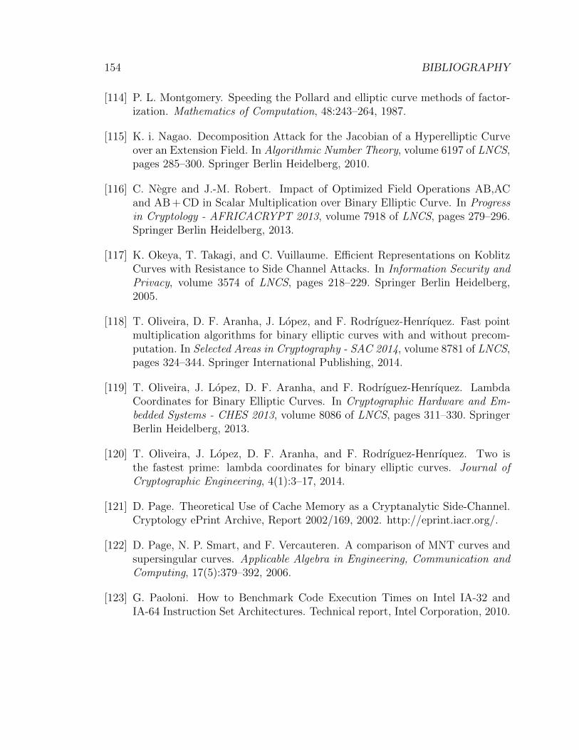
154 BIBLIOGRAPHY
[114] P. L. Montgomery. Speeding the Pollard and elliptic curve methods of factor-ization. Mathematics of Computation, 48:243–264, 1987.
[115] K. i. Nagao. Decomposition Attack for the Jacobian of a Hyperelliptic Curveover an Extension Field. In Algorithmic Number Theory, volume 6197 of LNCS,pages 285–300. Springer Berlin Heidelberg, 2010.
[116] C. Negre and J.-M. Robert. Impact of Optimized Field Operations AB,ACand AB + CD in Scalar Multiplication over Binary Elliptic Curve. In Progressin Cryptology - AFRICACRYPT 2013, volume 7918 of LNCS, pages 279–296.Springer Berlin Heidelberg, 2013.
[117] K. Okeya, T. Takagi, and C. Vuillaume. Efficient Representations on KoblitzCurves with Resistance to Side Channel Attacks. In Information Security andPrivacy, volume 3574 of LNCS, pages 218–229. Springer Berlin Heidelberg,2005.
[118] T. Oliveira, D. F. Aranha, J. Lopez, and F. Rodrıguez-Henrıquez. Fast pointmultiplication algorithms for binary elliptic curves with and without precom-putation. In Selected Areas in Cryptography - SAC 2014, volume 8781 of LNCS,pages 324–344. Springer International Publishing, 2014.
[119] T. Oliveira, J. Lopez, D. F. Aranha, and F. Rodrıguez-Henrıquez. LambdaCoordinates for Binary Elliptic Curves. In Cryptographic Hardware and Em-bedded Systems - CHES 2013, volume 8086 of LNCS, pages 311–330. SpringerBerlin Heidelberg, 2013.
[120] T. Oliveira, J. Lopez, D. F. Aranha, and F. Rodrıguez-Henrıquez. Two isthe fastest prime: lambda coordinates for binary elliptic curves. Journal ofCryptographic Engineering, 4(1):3–17, 2014.
[121] D. Page. Theoretical Use of Cache Memory as a Cryptanalytic Side-Channel.Cryptology ePrint Archive, Report 2002/169, 2002. http://eprint.iacr.org/.
[122] D. Page, N. P. Smart, and F. Vercauteren. A comparison of MNT curves andsupersingular curves. Applicable Algebra in Engineering, Communication andComputing, 17(5):379–392, 2006.
[123] G. Paoloni. How to Benchmark Code Execution Times on Intel IA-32 andIA-64 Instruction Set Architectures. Technical report, Intel Corporation, 2010.
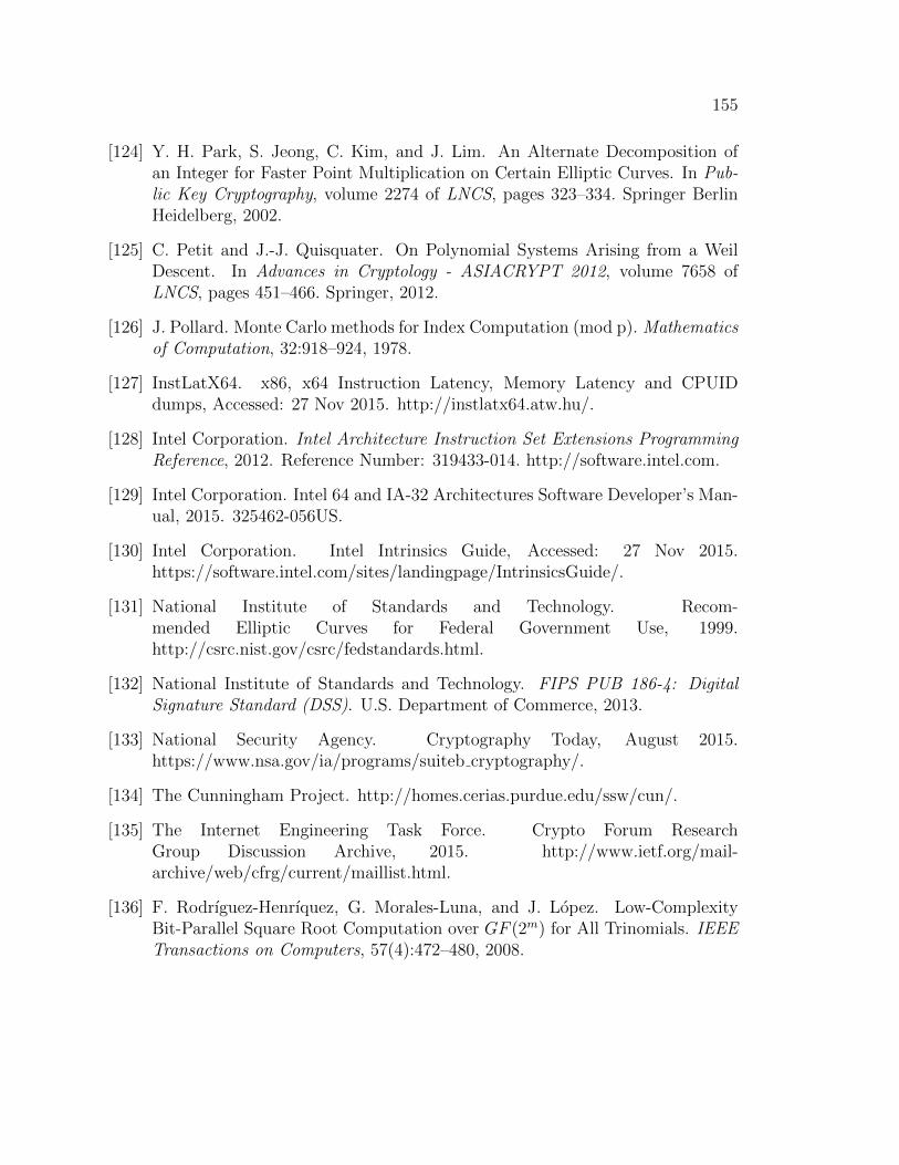
155
[124] Y. H. Park, S. Jeong, C. Kim, and J. Lim. An Alternate Decomposition ofan Integer for Faster Point Multiplication on Certain Elliptic Curves. In Pub-lic Key Cryptography, volume 2274 of LNCS, pages 323–334. Springer BerlinHeidelberg, 2002.
[125] C. Petit and J.-J. Quisquater. On Polynomial Systems Arising from a WeilDescent. In Advances in Cryptology - ASIACRYPT 2012, volume 7658 ofLNCS, pages 451–466. Springer, 2012.
[126] J. Pollard. Monte Carlo methods for Index Computation (mod p). Mathematicsof Computation, 32:918–924, 1978.
[127] InstLatX64. x86, x64 Instruction Latency, Memory Latency and CPUIDdumps, Accessed: 27 Nov 2015. http://instlatx64.atw.hu/.
[128] Intel Corporation. Intel Architecture Instruction Set Extensions ProgrammingReference, 2012. Reference Number: 319433-014. http://software.intel.com.
[129] Intel Corporation. Intel 64 and IA-32 Architectures Software Developer’s Man-ual, 2015. 325462-056US.
[130] Intel Corporation. Intel Intrinsics Guide, Accessed: 27 Nov 2015.https://software.intel.com/sites/landingpage/IntrinsicsGuide/.
[131] National Institute of Standards and Technology. Recom-mended Elliptic Curves for Federal Government Use, 1999.http://csrc.nist.gov/csrc/fedstandards.html.
[132] National Institute of Standards and Technology. FIPS PUB 186-4: DigitalSignature Standard (DSS). U.S. Department of Commerce, 2013.
[133] National Security Agency. Cryptography Today, August 2015.https://www.nsa.gov/ia/programs/suiteb cryptography/.
[134] The Cunningham Project. http://homes.cerias.purdue.edu/ssw/cun/.
[135] The Internet Engineering Task Force. Crypto Forum ResearchGroup Discussion Archive, 2015. http://www.ietf.org/mail-archive/web/cfrg/current/maillist.html.
[136] F. Rodrıguez-Henrıquez, G. Morales-Luna, and J. Lopez. Low-ComplexityBit-Parallel Square Root Computation over GF (2m) for All Trinomials. IEEETransactions on Computers, 57(4):472–480, 2008.
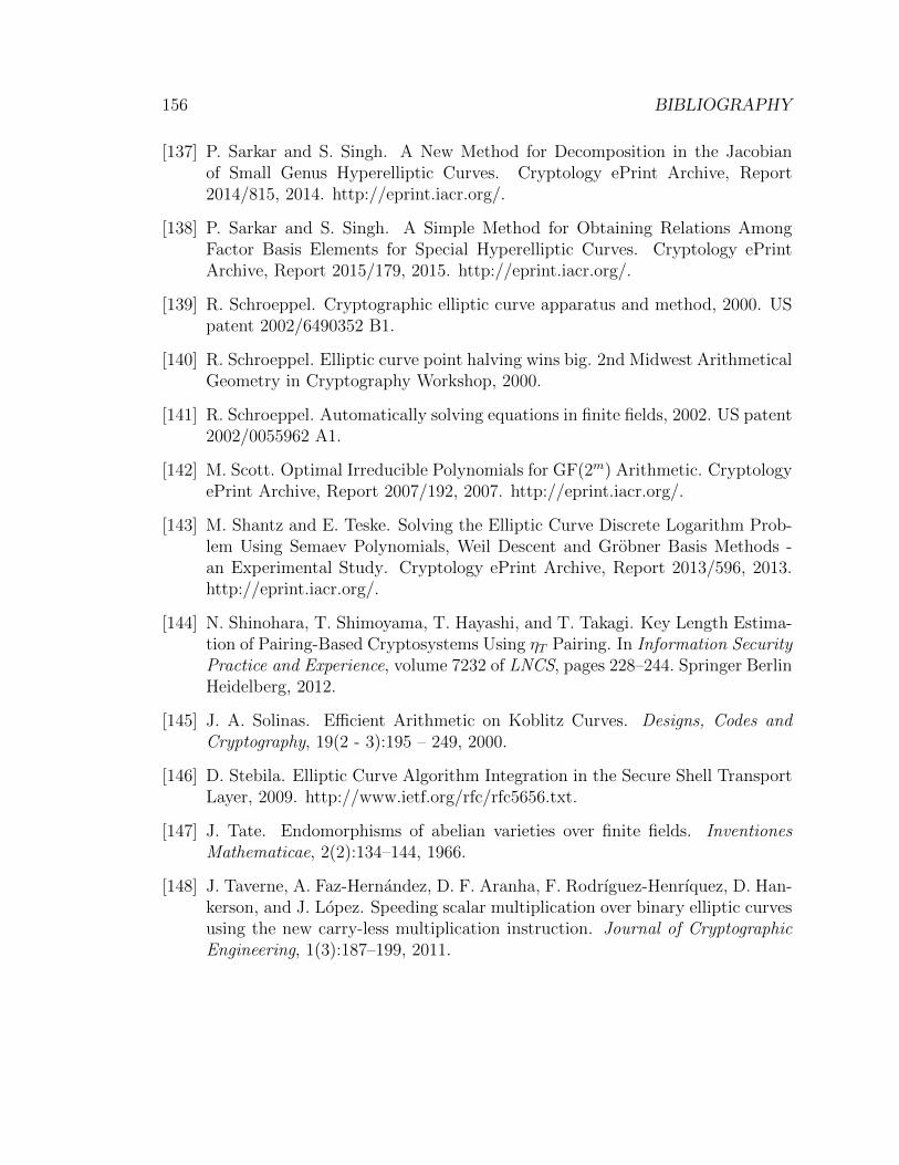
156 BIBLIOGRAPHY
[137] P. Sarkar and S. Singh. A New Method for Decomposition in the Jacobianof Small Genus Hyperelliptic Curves. Cryptology ePrint Archive, Report2014/815, 2014. http://eprint.iacr.org/.
[138] P. Sarkar and S. Singh. A Simple Method for Obtaining Relations AmongFactor Basis Elements for Special Hyperelliptic Curves. Cryptology ePrintArchive, Report 2015/179, 2015. http://eprint.iacr.org/.
[139] R. Schroeppel. Cryptographic elliptic curve apparatus and method, 2000. USpatent 2002/6490352 B1.
[140] R. Schroeppel. Elliptic curve point halving wins big. 2nd Midwest ArithmeticalGeometry in Cryptography Workshop, 2000.
[141] R. Schroeppel. Automatically solving equations in finite fields, 2002. US patent2002/0055962 A1.
[142] M. Scott. Optimal Irreducible Polynomials for GF(2m) Arithmetic. CryptologyePrint Archive, Report 2007/192, 2007. http://eprint.iacr.org/.
[143] M. Shantz and E. Teske. Solving the Elliptic Curve Discrete Logarithm Prob-lem Using Semaev Polynomials, Weil Descent and Grobner Basis Methods -an Experimental Study. Cryptology ePrint Archive, Report 2013/596, 2013.http://eprint.iacr.org/.
[144] N. Shinohara, T. Shimoyama, T. Hayashi, and T. Takagi. Key Length Estima-tion of Pairing-Based Cryptosystems Using ηT Pairing. In Information SecurityPractice and Experience, volume 7232 of LNCS, pages 228–244. Springer BerlinHeidelberg, 2012.
[145] J. A. Solinas. Efficient Arithmetic on Koblitz Curves. Designs, Codes andCryptography, 19(2 - 3):195 – 249, 2000.
[146] D. Stebila. Elliptic Curve Algorithm Integration in the Secure Shell TransportLayer, 2009. http://www.ietf.org/rfc/rfc5656.txt.
[147] J. Tate. Endomorphisms of abelian varieties over finite fields. InventionesMathematicae, 2(2):134–144, 1966.
[148] J. Taverne, A. Faz-Hernandez, D. F. Aranha, F. Rodrıguez-Henrıquez, D. Han-kerson, and J. Lopez. Speeding scalar multiplication over binary elliptic curvesusing the new carry-less multiplication instruction. Journal of CryptographicEngineering, 1(3):187–199, 2011.
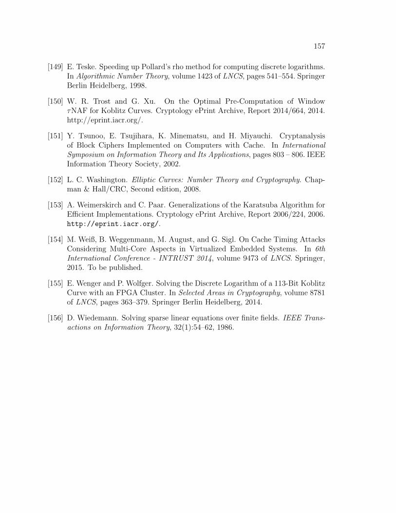
157
[149] E. Teske. Speeding up Pollard’s rho method for computing discrete logarithms.In Algorithmic Number Theory, volume 1423 of LNCS, pages 541–554. SpringerBerlin Heidelberg, 1998.
[150] W. R. Trost and G. Xu. On the Optimal Pre-Computation of WindowτNAF for Koblitz Curves. Cryptology ePrint Archive, Report 2014/664, 2014.http://eprint.iacr.org/.
[151] Y. Tsunoo, E. Tsujihara, K. Minematsu, and H. Miyauchi. Cryptanalysisof Block Ciphers Implemented on Computers with Cache. In InternationalSymposium on Information Theory and Its Applications, pages 803 – 806. IEEEInformation Theory Society, 2002.
[152] L. C. Washington. Elliptic Curves: Number Theory and Cryptography. Chap-man & Hall/CRC, Second edition, 2008.
[153] A. Weimerskirch and C. Paar. Generalizations of the Karatsuba Algorithm forEfficient Implementations. Cryptology ePrint Archive, Report 2006/224, 2006.http://eprint.iacr.org/.
[154] M. Weiß, B. Weggenmann, M. August, and G. Sigl. On Cache Timing AttacksConsidering Multi-Core Aspects in Virtualized Embedded Systems. In 6thInternational Conference - INTRUST 2014, volume 9473 of LNCS. Springer,2015. To be published.
[155] E. Wenger and P. Wolfger. Solving the Discrete Logarithm of a 113-Bit KoblitzCurve with an FPGA Cluster. In Selected Areas in Cryptography, volume 8781of LNCS, pages 363–379. Springer Berlin Heidelberg, 2014.
[156] D. Wiedemann. Solving sparse linear equations over finite fields. IEEE Trans-actions on Information Theory, 32(1):54–62, 1986.