centro de investigacion y de estudios avanzados … · dedicado a mi familia, a mi pap a francisco...

CENTRO DE INVESTIGACION Y DE ESTUDIOSAVANZADOS DEL INSTITUTO POLITECNICO NACIONAL

UNIDAD ZACATENCO

DEPARTAMENTO DE MATEMATICAS

Procesos de difusion en una dimensiony polinomios ortogonales

T E S I S

Que presenta

Jonathan Josue Gutierrez Pavon

Para obtener el grado de

MAESTRO EN CIENCIAS

EN LA ESPECIALIDAD DE

MATEMATICAS

Director de la tesis

Dr. Carlos Pacheco Gonzalez

Mexico, D. F. Febrero, 2015

CENTER FOR RESEARCH AND ADVANCED STUDIESOF THE NATIONAL POLYTECHNIC INSTITUTE

CAMPUS ZACATENCO

DEPARTMENT OF MATHEMATICS

One dimensional diffusion processesand orthogonal polynomials

T H E S I S

PRESENTED BY

Jonathan Josue Gutierrez Pavon

TO OBTAIN THE DEGREE OF

MASTER IN SCIENCE

IN THE SPECIALITY OF

MATHEMATICS

THESIS ADVISOR

Dr. Carlos Pacheco Gonzalez

Mexico, D. F. February , 2015

One dimensional diffusionprocesses and orthogonal

polynomials

Dedicado a mi familia,A mi papa Francisco Gutierrez Gutierrez,

A mi mama Isabel Pavon Hernandez,A mi hermana Rebeca Gutierrez Pavon,

Y a la familia Guzman Hernandez, porque son como una familia para mi.

Agradecimientos

Agradezco al Dr. Carlos Pacheco por toda la ayuda brindada, su interes en la elaboracion de estetrabajo, su dedicacion y paciencia.

A mis amigos y a mi familia, por todo el apoyo brindado.

Agradezco al Centro de Investigacion y Estudios Avanzados del Instituto Politecnico Nacional y alConsejo Nacional de Ciencia y Tecnologıa (CONACYT) por el apoyo economico proporcionadoque me permitio realizar este trabajo.

Tambien agradezco a la Universidad de Costa Rica por todo el apoyo brindado.

5

Abstract

We describe the general theory of diffusion processes, which contains as a particular case thesolutions of stochastic differential equations. The idea of the theory is to construct explicitly thegenerator of the Markov process using the so-called scale function and the speed measure. We alsoexplain how the theory of orthogonal polynomials help to study some diffusions. In addition, usingthe theory of diffusions, we present the Brox model, which is a process in a random environment.

Resumen

Describimos la teorıa general de procesos de difusion, que contiene como caso particular las solu-ciones de ecuaciones diferenciales estocasticas. La idea de la teorıa es construir explıcitamenteel generador de los procesos de Markov usando la suncion de escala y la medida de velocidad.Tambien explicamos como la teorıa de polinomios ortogonales ayuda a estudiar algunas difusiones.Ademas, usando la teoria de difusiones, presentamos el modelo de Brox, que es un proceso conambiente aleatorio.

Introduction

In the world where we live there are many natural phenomena that have a random character, andthe theory of probability is a tool that permits us to explain some of these events.

In this work, we will study the so-called diffusion processes in one dimension. The diffusionprocesses allow us to model some natural phenomena, such as random motion of particles. Adiffusion is a random process that has two important features: continuous paths and the Markovproperty. This last property is characterized by the loss of memory, which means that one canmake estimates of the future of the process based solely on its present state just as one could knowthe full history of the process. In other words, by conditioning on the present state of the system,its future and past are independent.

It turns out that a process Xt with the Markov property, is characterized by its infinitesimalgenerator, which is specified by the following operator

Af(x) := limt→0+

E(f(Xt)|X0 = x)− f(x)

tfor some functions f.

In this work we construct the infinitesimal generator using the scale function and the speedmeasure; these two objects characterize the infinitesimal generator. If (l, r), an interval in R,is the state space of the process Xt, then the scale function is the probability that the processfirst reaches r before l. On the other hand, the speed measure can be written in terms of theexpectation of the first time the process reaches either l or r.

Under appropriate assumptions on the scale function and the speed measure one can obtain thatthe infinitesimal generator can be written as a differential operator of order 2, also called a Sturm-Liouville operator, given by

Af(x) = µ(x)f ′(x) +σ2(x)

2f ′′(x), where µ and σ are certain functions.

This type of operators, with suitable conditions, are associated with diffusion processes that aresolutions of a stochastic differential equations. This differential operator has particular interestbecause it is related to some orthogonal polynomials. More precisely, if we consider the functionsµ(x) and σ2(x) to be polynomials of degree at most 1 and 2 respectively, then there exist orthogonalpolynomials that are eigenfunctions of the operator, and the process associated with this operatorhas a density probability function that can be written in terms of these orthogonal polynomials.

In this work, we also study an example of a diffusion whose infinitesimal generator is not a Sturm-Liouville operator. What one has to do is to construct explicitly the scale function and the speedmeasure. The process we consider is called the Brox diffusion [11], and it is an example of aprocess in a random environment. The importance of this type of processes is that it considersthe random medium.

9

10

This thesis is mainly based on Chapter VII of D. Revuz, and M. Yor. [3]. In chapter 1, we showin detail the results that allow us to write the infinitesimal generator of a diffusion process X interms of the scale function s and the speed measure m. We prove the following result

d

dm

d

dsf+ =

d

dm

d

dsf− = lim

t→0+

E(f(Xt)|X0 = x)− f(x)

t,

where on the left hand side we have derivatives with respect to the function s and the measure m.

In chapter 2 we present the main result on orthogonal polynomials that we use in chapter 3. Inchapter 3 we characterize the probability density of the Ornstein-Uhlenbeck, the Cox-Ingersoll-Rossand Jacobi diffusions through Hermite, Laguerre and Jacobi orthogonal polynomials respectively.At the end of chapter 3 we give an example of a diffusion that does not fit in the classical context:the Brox diffusion, which is a diffusion in a random environment.

Contents

Introduction 9

1 Diffusion processes in one dimension 151.1 Notation . . . . . . . . . . . . . . . . . . . . . . . . . . . . . . . . . . . . . . . . . . 151.2 Diffusion process . . . . . . . . . . . . . . . . . . . . . . . . . . . . . . . . . . . . . 161.3 The scale function . . . . . . . . . . . . . . . . . . . . . . . . . . . . . . . . . . . . 181.4 The speed measure . . . . . . . . . . . . . . . . . . . . . . . . . . . . . . . . . . . . 211.5 Infinitesimal operator . . . . . . . . . . . . . . . . . . . . . . . . . . . . . . . . . . 291.6 A particular classic case . . . . . . . . . . . . . . . . . . . . . . . . . . . . . . . . . 36

2 Orthogonal polynomials in one dimension 432.1 Orthogonal polynomials . . . . . . . . . . . . . . . . . . . . . . . . . . . . . . . . . 432.2 The derivative of orthogonal polynomials . . . . . . . . . . . . . . . . . . . . . . . 452.3 A differential equation for the orthogonal polynomials . . . . . . . . . . . . . . . . 462.4 Classical orthogonal polynomials . . . . . . . . . . . . . . . . . . . . . . . . . . . . 482.5 The formula of Rodrigues type . . . . . . . . . . . . . . . . . . . . . . . . . . . . . 492.6 Completeness of the orthogonal polynomials . . . . . . . . . . . . . . . . . . . . . . 51

2.6.1 Hermite polynomials . . . . . . . . . . . . . . . . . . . . . . . . . . . . . . . 512.6.2 Jacobi polynomials . . . . . . . . . . . . . . . . . . . . . . . . . . . . . . . 52

2.7 Example: Hermite polynomials . . . . . . . . . . . . . . . . . . . . . . . . . . . . . 532.7.1 The three terms recurrence relation . . . . . . . . . . . . . . . . . . . . . . 532.7.2 Orthogonality of the Hermite polynomials . . . . . . . . . . . . . . . . . . . 54

3 Diffusions and orthogonal polynomials 573.1 The Ornstein-Uhlenbeck process . . . . . . . . . . . . . . . . . . . . . . . . . . . . 573.2 The Cox-Ingersoll-Ross process . . . . . . . . . . . . . . . . . . . . . . . . . . . . . 593.3 The Jacobi process . . . . . . . . . . . . . . . . . . . . . . . . . . . . . . . . . . . . 603.4 The Brox process . . . . . . . . . . . . . . . . . . . . . . . . . . . . . . . . . . . . . 61

Bibliography 66

11

12 CONTENTS

Chapter 1

Diffusion processes in onedimension

1.1 Notation

1. The symbol θt represents a transformation such that the effect on a path ω := ω(s)s≥0 isthe following θt(ω) = ω(s)s≥t. This transformation is called the shift operator and hasthe properties

(a) Xt(θs(ω)) = Xt+s(ω) for all stochastic process X := Xt : t ≥ 0 and

(b) θt θs = θt+s.

2. The expression an a means that the sequence an converges to a, and an ≤ an+1 for all n.Similarly an a means that the sequence an converges to a, and an ≥ an+1 for all n.

3. Let X := Xt : t ≥ 0 be a Markov process with state space E, and A ⊆ E measurable,then Px(Xt ∈ A) := P (Xt ∈ A | X0 = x) and Ex(Xt) := E(Xt | X0 = x). Also, p(t, x, dy)

represents the transition probability distribution, i.e. P (Xt ∈ A|X0 = x) =

∫A

p(t, x, dy).

1.2 Diffusion process

In this section we will look at some basic concepts about diffusions.

Definition 1.2.1. Let E = (l, r) be an interval of R which may be closed, open, semi open, boundedor unbounded.

1. The hitting time of a one-point set x is denote by Tx, and defined by

Tx := inft > 0 : Xt = x.

2. A stochastic process X = X(t), t ≥ 0 with state space E is called a diffusion process ifit satisfies the following:

(a) The paths of X are continuous.

13

14 CHAPTER 1. DIFFUSION PROCESSES IN ONE DIMENSION

(b) X enjoys the strong Markov property, i.e. for F : Ω → R measurable and τ a stoppingtime, then

Ex(F (X θτ )|Fτ ) = EXτ (F (X)).

(c) X is regular, i.e. for any x ∈ int(E) and y ∈ E, Px(Ty <∞) > 0.

3. For any interval I = (a, b) such that [a, b] ⊆ E, we denote by σI the exit time of I, i.e.σI := Ta ∧ Tb. We also write mI(x) := Ex(σI).

Theorem 1.2.2. If I is bounded, the function mI is bounded on I.

Proof. Note that for any fixed y in I, we may pick α < 1 and t > 0 such that

maxPy(Ta > t), Py(Tb > t) = α. (1.1)

From the regularity of X, Py(Ta <∞) > 0, then

0 < Py(Ta <∞) = Py

( ∞⋃n=0

Ta < n

)≤∞∑n=0

Py (Ta < n) .

Consequently there exists an n0 such that Py(Ta < n0) > 0. Thus Py(Ta > n0) < 1, and by thesame procedure we obtain an m0 such that Py(Tb > m0) < 1. Now, define t := maxn0,m0 andα := maxPy(Ta > n0), Py(Tb > m0).

We will prove thatsupx∈I

Px(σI > t) ≤ α. (1.2)

Let y be a fixed point in I. If y < x < b then

Px(σI > t) ≤ Px(Tb > t) ≤ Py(Tb > t) ≤ α < 1.

The second inequality is because any path that starts in y has to pass through x.

Similarly if a < x < y, then

Px(σI > t) ≤ Px(Ta > t) ≤ Py(Ta > t) ≤ α < 1,

which yields (1.2).

Now, since σI = u+ σI θu on σI > u, we have

Px(σI > nt) = Px(σI > (n− 1)t, σI > nt)

= Px(σI > (n− 1)t, (n− 1)t+ σI θ(n−1)t > nt)

= Ex

(1σI>(n−1)t · 1(n−1)t+σIθ(n−1)t>nt

)= Ex

(1σI>(n−1)t · 1σIθ(n−1)t>t

)= Ex

(1σI>(n−1)t · 1σI>t θ(n−1)t

)(Markovproperty

)= Ex

(1σI>(n−1)t · EX(n−1)t

(1σI>t)).

1.3. THE SCALE FUNCTION 15

Since σI > (n− 1)t, then X(n−1)t ∈ I and, by (1.2), we obtain

EX(n−1)t

(1σI>t) ≤ α.

Therefore Px(σI > nt) ≤ αPx (σI > (n− 1)t).

Recursively it follows that

Px(σI > nt) ≤ αn. (1.3)

On the other hand, we know that Ex(σI) ≤∞∑n=0

t Px(σI > nt). Hence

Ex(σI) ≤∞∑n=0

tαn = t(1− α)−1 <∞.

Remark: For a and b in E and l ≤ a < x < b ≤ r, the probability Px(Tb < Ta) is the probabilitythat the process started at x exits (a, b) by its right end. We also have that

Px(Tb < Ta) + Px(Ta < Tb) = 1.

1.3 The scale function

Theorem 1.3.1. There exists a continuous, strictly increasing function s on E such that

Px(Tb < Ta) =s(x)− s(a)

s(b)− s(a). (1.4)

for any a, b, x in E with l ≤ a < x < b ≤ r. Also if s is another function with the same properties,then s = αs+ β with α > 0 and β ∈ R.

Proof. The event Tr < Tl is equal to the disjoint union

Tr < Tl, Ta < Tb⋃Tr < Tl, Tb < Ta.

Note that Tl = Ta + Tl θTa always, and Tr = Ta + Tr θTa on the set Ta < Tb. Then by theMarkov property we have

Px (Tr < Tl, Ta < Tb) = Ex(1Tr<Tl · 1Ta<Tb

)= Ex

(1Ta+TrθTa<Ta+TlθTa · 1Ta<Tb

)= Ex

(1Tr<Tl θTa · 1Ta<Tb

)(Markovproperty

)= Ex

(EXTa (1Tr<Tl) · 1Ta<Tb

).


Since XTa = a, then EXTa (1Tr<Tl) = Ea(1Tr<Tl), thus

Px (Tr < Tl, Ta < Tb) = Ex(Ea(1Tr<Tl) · 1Ta<Tb

)= Ea(1Tr<Tl) · Ex(1Ta<Tb)

= Pa(Tr < Tl) · Px(Ta < Tb).

We finally obtain

Px(Tr < Tl) = Pa(Tr < Tl) · Px(Ta < Tb) + Pb(Tr < Tl) · Px(Tb < Ta). (1.5)

Define s(x) := Px(Tr < Tl), and solving for Px(Tb < Ta) we obtain the formula in the statement.

Let us now verify first s is increasing. Indeed, because the paths of X are continuous

Px(Tr < Tl) ≤ Py(Tr < Tl) if x < y.

We now see that s is strictly increasing. Suppose there exists x < y such that s(x) = s(y). Thenfor any b > y, by (1.4) we obtain

Py(Tb < Tx) =s(y)− s(x)

s(b)− s(x)= 0.

This contradicts the regularity of the process. Therefore s is strictly increasing.

We now will prove that s is continuous. To this end, we first prove that

limn→∞

Px(Tan < Tb) = Px(Ta < Tb), if an a. (1.6)

Note that if a < x and an a then Tan Ta if X(0) = x.

We know that XTa = a if X(0) = x. Then

Px(Ta < Tb) = Px

( ∞⋂n=1

Tan < Tb

)= limn→∞

Px(Tan < Tb),

because Tan+1 < Tb ⊆ Tan < Tb.

On the other hand, if l ≤ a < x < b ≤ r we know that it holds the equality (1.5).

Suppose that y ∈ E, and consider yn y (the case yn y is similar).

We will see that s(yn)→ s(y). Take b ∈ E such that l ≤ y < yn < b ≤ r. By (1.5) we know that

Py(Tb < Tyn) =s(y)− s(yn)

s(b)− s(yn).

Then

0 = limn→∞

Py(Tb < Tyn) = limn→∞

s(y)− s(yn)

s(b)− s(yn). (1.7)

Since yn y and s is strictly increasing, s(yn) > s(yn+1) > ... > s(y), so the sequence s(yn)is decreasing and bounded by s(y). Therefore there exists α such that s(yn) → α and s(b) > α.Hence by (1.7) we obtain that s(yn)→ s(y).

1.4. THE SPEED MEASURE 17

Suppose now that s is another function such that s is continuous, strictly increasing, and

Px(Tb < Ta) =s(x)− s(a)

s(b)− s(a),

then we will prove s = αs+ β, for some α > 0, β ∈ R.

Let l ≤ a < x < b ≤ r, from (1.5)

Px(Tr < Tl) = Px(Ta < Tb)Pa(Tr < Tl) + Px(Tb < Ta)Pb(Tr < Tl), (1.8)

where, by definition, s(x) = Px(Tr < Tl) and Px(Tb < Ta) =s(x)− s(a)

s(b)− s(a). Then by (1.8) we obtain

s(x) =s(b)− s(x)

s(b)− s(a)· Pa(Tr < Tl) +

s(x)− s(a)

s(b)− s(a)· Pb(Tr < Tl).

Therefore s = αs+ β, with

α :=s(b)− s(a)

Pb(Tr < Tl)− Pa(Tr < Tl), β :=

s(a)Pb(Tr < Tl)− s(b)Pa(Tr < Tl)

Pb(Tr < Tl)− Pa(Tr < Tl).

Definition 1.3.2. The function s of the Theorem 1.3.1 is called the scale function of the processX. In particular we say that X is on its natural or standard scale if s(x) = x.

Note that if a process X has scale function s, then the process Y := s(X) is on its natural scale.

1.4 The speed measure

Definition 1.4.1. Let s be a continuous function and strictly increasing on [l, r]. A function f iscalled s-convex if for l ≤ a < x < b ≤ r

(s(b)− s(a))f(x) ≤ (s(b)− s(x))f(a) + (s(x)− s(a))f(b). (1.9)

Define also the right and left s-derivativesdf+

dsand

df−ds

as

df+

ds(x) := lim

y→x+

f(y)− f(x)

s(y)− s(x), and

df−ds

(x) := limy→x−

f(x)− f(y)

s(x)− s(y). (1.10)

At the points where they coincide we say that f has an s-derivative.

If m is a measure, then we define the m-derivative of f at x as

df

dm(x) := lim

y→x+

f(y)− f(x)

m((x, y]).

Lemma 1.4.2. Let s be a continuous function and strictly increasing on [l, r]. If f is s-convex,then f is continuous on [l, r].


Proof. Since f is s-convex, if l ≤ u < w < v ≤ r, then

(s(v)− s(u))f(w) ≤ (s(w)− s(u))f(v) + (s(v)− s(w))f(u).

This impliesf(w)− f(u)

s(w)− s(u)≤ f(v)− f(u)

s(v)− s(u)≤ f(v)− f(w)

s(v)− s(w). (1.11)

Now, let x ∈ (l, r) and pick v ∈ (l, r) such that l ≤ x < v ≤ r, and apply (1.11) to obtain

f(x)− f(l)

s(x)− s(l)≤ f(v)− f(x)

s(v)− s(x)≤ f(r)− f(x)

s(r)− s(x). (1.12)

By (1.12) we obtain

f(x)− f(l)

s(x)− s(l)· (s(v)− s(x)) + f(x) ≤ f(v) ≤ f(r)− f(x)

s(r)− s(x)· (s(v)− s(x)) + f(x). (1.13)

Take v x in (1.13) to see that limv→x+

f(v) = f(x). Therefore f is right continuous. Left continuity

is shown in exactly the same way.

Lemma 1.4.3. Let s be a continuous function and strictly increasing on [l, r]. If f is a function

s-convex on [l, r], thendf+

dsand

df−ds

are increasing, thus of bounded variation.

Proof. Let l ≤ x < y ≤ r, and pick xn, yn such that l ≤ x < xn < y < yn ≤ r.

Since f is s-convex then

f(xn)− f(x)

s(xn)− s(x)≤ f(y)− f(xn)

s(y)− s(xn)≤ f(yn)− f(y)

s(yn)− s(y). (1.14)

From (1.14) we obtain

f(xn)− f(x)

s(xn)− s(x)≤ f(yn)− f(y)

s(yn)− s(y).

Finally take xn → x and yn → y.

Lemma 1.4.4. Let f be a function s-convex on I = [a, b] and f(a) = f(b) = 0. Then there exists

a measure µ such that µ((c, d]) =df+

ds(d)− df+

ds(c), and

f(x) = −∫ b

a

GI(x, y) µ(dy),

where

GI(x, y) :=

(s(x)− s(a))(s(b)− s(y))

s(b)− s(a), a ≤ x ≤ y ≤ b,

(s(y)− s(a))(s(b)− s(x))

s(b)− s(a), a ≤ y ≤ x ≤ b,

0, otherwise.

GI is called the Green function.


Proof. Using the integration by parts formula for Stieltjes integrals we obtain∫ b

a

GI(x, y) µ(dy) =

∫ b

a

GI(x, y) d

(df+

ds(y)

)=

s(b)− s(x)

s(b)− s(a)

∫ x

a

(s(y)− s(a)) d

(df+

ds(y)

)+

s(x)− s(a)

s(b)− s(a)

∫ b

x

(s(b)− s(y)) d

(df+

ds(y)

)=

s(b)− s(x)

s(b)− s(a)

((s(x)− s(a))

df+

ds(x)−

∫ x

a

df+

ds(y) ds(y)

)+

s(x)− s(a)

s(b)− s(a)

((s(x)− s(b))df+

ds(x)−

∫ b

x

df+

ds(y) ds(y)

)

=s(b)− s(x)

s(b)− s(a)(f(a)− f(x)) +

s(x)− s(a)

s(b)− s(a)(f(x)− f(b))

= −f(x).

Theorem 1.4.5. There exists a unique measure m such that for all I = (a, b)

mI(x) =

∫ b

a

GI(x, y) m(dy) =

∫ b

a

GI(x, y) d

(−d(mI(y))+

ds

),

with [a, b] ⊆ E, and where GI is the Green function.

Proof. We apply the Lemma 1.4.4. We will first show that −mI is s-convex. Let a < c < x < d < b,and J := (c, d), I := (a, b). Then by the Markov property we obtain

mI(x) = Ex (σI)

(σI=σJ+σIθσJ )= Ex (σJ + σI θσJ )

= mJ(x) + Ex (σI θσJ )

= mJ(x) + Ex (σI θσJ )(Markovproperty

)= mJ(x) + Ex

(EXσJ (σI)

)= mJ(x) + Ex

(EXσJ (σI) · 1Tc<Td

)+ Ex

(EXσJ (σI) · 1Td<Tc

)= mJ(x) + Ex

(EXTc (σI) · 1Tc<Td

)+ Ex

(EXTd (σI) · 1Td<Tc

)= mJ(x) + Ex

(Ec (σI) · 1Tc<Td

)+ Ex

(Ed (σI) · 1Td<Tc

)= mJ(x) + Ec (σI) · Ex

(1Tc<Td

)+ Ed (σI) · Ex

(1Td<Tc

)= mJ(x) + Ec (σI) · Px (Tc < Td) + Ed (σI) · Px (Td < Tc)

= mJ(x) +mI(c) ·(s(d)− s(x)

s(d)− s(c)

)+mI(d) ·

(s(x)− s(c)s(d)− s(c)

). (1.15)


Hence if follows that −mI is s-convex. Also, mI(a) = mI(b) = 0. Then by Lemma 1.4.4 there

exists a measure m with m(dy) := d(−d(mI(y))+

ds

), such that

mI(x) =

∫ b

a

GI(x, y) m(dy) =

∫ b

a

GI(x, y) d

(−d(mI(y))+

ds

).

Let us check the uniqueness of m. Let J := (c, d) ⊆ I := (a, b). If we consider the functions mI(x)and mJ(x), and we apply the Theorem 1.4.5, then there exist measures m and m such that

m(dy) = d

(−d(mI(y))+

ds

), and m(dy) = d

(−d(mJ(y))+

ds

).

However, if we calculate the s-derivative in both side of (1.15), we obtain

d(mI(y))+

ds=d(mJ(y))+

ds+ C,

where C is a constant, in particular this holds for J = I. Therefore m = m.

Corollary 1.4.6. The measure m satisfies that

m((w, z]) =

(−d(mI(z))+

ds

)−(−d(mI(w))+

ds

).

Definition 1.4.7. The measure m of the Theorem 1.4.5 is called the speed measure of the processX.

Lemma 1.4.8. If v(x) := Ex

(∫ Ta∧Tb

0

1(c,b) Xudu

), then

v(x) =

Ex(Tc ∧ Tb) + Px(Tc < Tb) · v(c), x ∈ (c, b),Px(Tc < Ta) · v(c), x ∈ (a, c].

In particular if x ∈ (c, b) we havedv+

ds=dEx(Tc ∧ Tb)+

ds+ C, where C is a constant.

Proof. Let x ∈ (c, b), and define now σJ := Tc ∧ Tb. By the Markov property we obtain

Px(Tc < Tb) · v(c) = Ex(1Tc<Tb

)· Ec

(∫ σI

0

1(c,b) Xu du

)= Ex

(1Tc<Tb · Ec

(∫ σI

0

1(c,b) Xu du

))(c=XTc=XσJ )

= Ex

(1Tc<Tb · EXσJ

(∫ σI

0

1(c,b) Xu du

))(Markovproperty

)= Ex

(1Tc<Tb ·

(∫ σI

0

1(c,b) Xu du

) θσJ

)= Ex

(1Tc<Tb ·

(∫ σIθσJ

0

1(c,b) Xu θσJ du

))

= Ex

(1Tc<Tb ·

∫ σI

σJ

1(c,b) Xu du

).


On the other hand, since x ∈ (c, b) we have

Ex(Tc ∧ Tb) = Ex(1Tc<Tb · (Tc ∧ Tb)

)+ Ex

(1Tb<Tc · (Tc ∧ Tb)

)= Ex

(1Tc<Tb ·

∫ σJ

0

du

)+ Ex

(1Tb<Tc ·

∫ σJ

0

du

)( σJ=σIon Tb<Tc

)= Ex

(1Tc<Tb ·

∫ σJ

0

1(c,b) Xu du

)+ Ex

(1Tb<Tc ·

∫ σI

0

1(c,b) Xu du

).

Therefore if x ∈ (c, b), then Ex(Tc ∧ Tb) + Px(Tc < Tb) · v(c) equals

Ex

(1Tc<Tb ·

∫ σI

0

1(c,b) Xu du

)+ Ex

(1Tb<Tc ·

∫ σI

0

1(c,b) Xu du

)= v(x). (1.16)

In the same way we obtain that, if x ∈ (a, c] then

v(x) = Px(Tc < Ta) · v(c). (1.17)

Combining (1.16) and (1.17), we arrive at the equality

v(x) = [Ex(Tc ∧ Tb) + Px(Tc < Tb) · v(c)] · 1(c,b) + Px(Tc < Ta) · v(c) · 1(a,c]

=

[Ex(Tc ∧ Tb) +

s(b)− s(x)

s(b)− s(c)· v(c)

]· 1(c,b) +

s(x)− s(a)

s(c)− s(a)· v(c) · 1(a,c]

= Ex(Tc ∧ Tb) · 1(c,b) +s(b)− s(x)

s(b)− s(c)· v(c) · 1(c,b) +

s(x)− s(a)

s(c)− s(a)· v(c) · 1(a,c].

In the following, C0(R) will denote the space of the continuous functions that vanish at infinity.

Corollary 1.4.9. If I = (a, b), x ∈ I, f ∈ C0(R), then

Ex

(∫ Ta∧Tb

0

f (Xs) ds

)=

∫ b

a

GI(x, y)f(y)m(dy). (1.18)

Proof. Let c ∈ (a, b). We will now prove that the function v(x) := Ex

(∫ Ta∧Tb

0

1(c,b) Xudu

)is

s-concave on (a, b). So −v(x) is s-convex.

We will show that

Px(Tm < Tn) · v(m) + Px(Tn < Tm) · v(n) ≤ v(x),

where a < m < x < n < b, which means that v is s-concave. Let σJ := Tm ∧Tm and σI := Ta ∧Tb,


then σI = σJ + σI θσJ . Note that by the Markov property

Px(Tm < Tn) · v(m) = Ex(1Tm<Tn

)· Em

(∫ Ta∧Tb

0

1(c,b) Xu du

)

= Ex

(1Tm<Tn · Em

(∫ σI

0

1(c,b) Xu du

))(m=XTm=XσJ )

= Ex

(1Tm<Tn · EXσJ

(∫ σI

0

1(c,b) Xu du

))(Markovproperty

)= Ex

(1Tm<Tn ·

(∫ σI

0

1(c,b) Xu du

) θσJ

)= Ex

(1Tm<Tn ·

∫ σIθσJ

0

1(c,b) Xu θσJ du

)

= Ex

(1Tm<Tn ·

∫ σJ+σIθσJ

σJ

1(c,b) Xu du

)(σJ+σIθσJ=σI)

= Ex

(1Tm<Tn ·

∫ σI

σJ

1(c,b) Xu du

).

In the same way we obtain that

Px(Tn < Tm) · v(n) = Ex

(1Tn<Tm ·

∫ σI

σJ

1(c,b) Xu du

).

Then

Px(Tm < Tn) · v(m) + Px(Tn < Tm) · v(n) = Ex

(∫ σI

σJ

1(c,b) Xu du

)≤ Ex

(∫ σI

0

1(c,b) Xu du

)= v(x).

So −v is s-convex and v(a) = v(b) = 0. Therefore, applying the Lemma 1.4.4, there exists a

measure µ such that µ(dy) = −d(dv+

ds(y)

)and

v(x) =

∫ b

a

GI(x, y) µ(dy) = −∫ b

a

GI(x, y) d

(dv+

ds(y)

). (1.19)

Then by Lemma 1.4.8 we arrive to

v(x) = −∫GI(x, y) 1(c,b) d

(dEy(Tc ∧ Tb)+

ds

)=

∫GI(x, y) 1(c,b) m(dy),

where m is the speed measure.

1.5 Infinitesimal operator

The purpose of this section is to prove that the scale function and the speed measure characterizethe infinitesimal operator of the diffusion process X. We will appeal to some standard results ofthe theory of semigroups (see e.g. [3]).

1.5. INFINITESIMAL OPERATOR 23

In the following, Pt will denote the semigroup Pt(f)(x) := E(f(Xt)|X0 = x).

Definition 1.5.1. Let X be a diffusion process. A function f ∈ C0(R) is said to belong to thedomain DA of the infinitesimal operator of X if the limit

Af = limt→0+

Ptf − ft

(1.20)

exists in C0(R). This operator A : DA → C0(R) is called the infinitesimal operator of theprocess X or of the semigroup Pt.

By the properties of the Markov process, if f ∈ C0(R) then

E(f(Xt+h) | Ft) = Ph(f(Xt)), (1.21)

where Ft := σ(Xs : s ≤ t).

The following result which is useful for our purposes can be found in [3, p.282].

Lemma 1.5.2. If f ∈ DA, then:

1. The function t→ Ptf is differentiable in C0(R) and

d

dtPtf = APtf = PtAf.

2. Ptf − f =

∫ t

0

PsAf ds.

Lemma 1.5.3. For all y ∈ E we have that

α := Ey

(f(Xt−s)− f(X0)−

∫ t−s

0

Af(Xu)du

)= 0, (1.22)

Proof.

α = Ey(f(Xt−s))− f(y)− Ey(∫ t−s

0

Af(Xu)du

)= Ey (E(f(Xt−s)| F0))− f(y)− Ey

(E

(∫ t−s

0

Af(Xu)du

∣∣∣∣ F0

))(

(1.21) andFubini

)= Ey(Pt−sf(X0))− f(y)− Ey

(∫ t−s

0

E(Af(Xu) |F0) du

)(1.21)

= Pt−sf(y)− f(y)− Ey(∫ t−s

0

PuAf(X0) du

)= Pt−sf(y)− f(y)−

∫ t−s

0

PuAf(y) du

(Lemma 1.5.2)= 0.


Theorem 1.5.4. Let X0 := x. If f ∈ DA, then the process

Mft := f(Xt)− f(X0)−

∫ t

0

Af(Xs) ds,

is a martingale with respect to Ftt≥0 for every x.

Proof. Since f and Af are bounded, one can check that Mft is integrable for each t. Now, let

s < t, by the Markov property we have

Ex(Mft | Fs) = Ex

(f(Xt)− f(X0)−

∫ t

0

Af(Xu) du

∣∣∣∣ Fs)(adding ±f(Xs))

= Mfs + Ex

(f(Xt)− f(Xs)−

∫ t

s

Af(Xu)du

∣∣∣∣ Fs)= Mf

s + Ex

(f(Xt−s)− f(X0)−

∫ t−s

0

Af(Xu)du

θs

∣∣∣∣Fs)(Markovproperty

)= Mf

s + EXs

(f(Xt−s)− f(X0)−

∫ t−s

0

Af(Xu)du

)(Lemma 1.5.3)

= Mfs .

Therefore Mft is a martingale with respect to Ftt≥0.

Theorem 1.5.5. Let f ∈ DA and x in the interior of E. Then the s-derivative of f exists exceptpossibly on the set x : m(x) > 0.

Proof. Let f ∈ DA, σI := Ta ∧ Tb and x ∈ (a, b) such that [a, b] ⊆ E.

By Theorem 1.5.4, we know that Mft is a martingale with respect to Ftt≥0. Also |Mf

t | ≤ α+t ·β.

This implies that |Mft∧σI | ≤ α+ σI · β.

Define S := α+ σI · β. By Theorem 1.2.2 we have that Ex(σI) <∞, which implies Ex(S) <∞.

Let us prove that Mft∧σI is uniformly integrable. Indeed

limc→∞

supt

∫|Mf

t∧σI|>c

∣∣Mft∧σI

∣∣dP ≤ limc→∞

supt

∫|S|>c

∣∣S|dP= lim

c→∞

∫|S|>c

∣∣S|dP= 0.

By Doob optional stopping theorem (see e.g. [2, p.87]) , we have that Ex(MfσI ) = Ex(Mf

0 ) = 0, so

Ex(f(XσI ))− f(x) = Ex

(∫ σI

0

Af(Xs) ds

).

Now, by Corollary 1.4.9 we obtain

Ex(f(XσI ))− f(x) = Ex

(∫ σI

0

Af(Xs) ds

)=

∫ b

a

GI(x, y)Af(y) m(dy). (1.23)


On the other hand, we have that

Ex (f(XσI )) = Ex(f(XσI ) · 1Ta<Tb

)+ Ex(f(XσI ) · 1Tb<Ta)

= Ex(f(XTa) · 1Ta<Tb) + Ex(f(XTb) · 1Tb<Ta)= Ex(f(a) · 1Ta<Tb) + Ex(f(b) · 1Tb<Ta)= f(a) · Ex(1Ta<Tb) + f(b) · Ex(1Tb<Ta)

= f(a) · Px(Ta < Tb) + f(b) · Px(Tb < Ta)

= f(a) · s(b)− s(x)

s(b)− s(a)+ f(b) · s(x)− s(a)

s(b)− s(a). (1.24)

Then substituting in (1.24) in the equation (1.23) we arrive at

f(a) · s(b)− s(x)

s(b)− s(a)+ f(b) · s(x)− s(a)

s(b)− s(a)− f(x) =

∫ b

a

GI(x, y)Af(y)m(dy). (1.25)

By the definition of Green function we have for every x ∈ (a, b) that∫ b

a

GI(x, y)Af(y) m(dy) =s(b)− s(x)

s(b)− s(a)·∫ x

a

(s(y)− s(a))Af(y)m(dy)

+s(x)− s(a)

s(b)− s(a)·∫ b

x

(s(b)− s(y))Af(y)m(dy). (1.26)

Replacing (1.26) in the equation (1.25) and simplifying we obtain

f(b)− f(x)

s(b)− s(x)− f(x)− f(a)

s(x)− s(a)= J1 + J2, (1.27)

where

J1 :=

∫ x

a

s(y)− s(a)

s(x)− s(a)Af(y)m(dy).

J2 :=

∫ b

x

s(b)− s(y)

s(b)− s(x)Af(y)m(dy).

If we take b x in the equality (1.27) and we apply the theorem of differentiation of Lebesgue to

J2 ·m((x, b])

m((x, b]), then

df+

ds(x)− f(x)− f(a)

s(x)− s(a)=

∫ x

a

s(y)− s(a)

s(x)− s(a)Af(y)m(dy) +m(x)Af(x).

In the same manner, in this last equality we take a x, which yields

df+

ds(x)− df−

ds(x) = 2m(x)Af(x).

Therefore the s-derivative of f exists except possibly on the set x : m(x) > 0.


Corollary 1.5.6. The s-derivative of f ∈ DA exists for almost every x ∈ R.

Proof. Note that by construction of the speed measure m we known that

m((w, z]) = −dEz(σI)+

ds+dEw(σI)+

ds,

Since −mI(x) := −Ex(σI) is s-convex, then−Ex(σI)+

dsis increasing, and so

−Ex(σI)+

dsis contin-

uous except possibly in a countable set. Therefore m(x) = 0 for almost every x ∈ R. By theTheorem 1.5.5we obtain that the s-derivative of f ∈ DA exists for almost every x ∈ R.

The following result resembles the fundamental theorem of calculus.

Theorem 1.5.7. Let f ∈ DA, then∫ x+h

x

Af(y)m(dy) =df+

ds(x+ h)− df+

ds(x). (1.28)

Proof. Since the formula (1.25) is valid for all x ∈ (a, b), pick h > 0 such that x + h ∈ (a, b), andapply the formula to obtain

∫ b

a

GI(x+ h, y)Af(y)m(dy) = f(a) · s(b)− s(x+ h)

s(b)− s(a)+ f(b) · s(x+ h)− s(a)

s(b)− s(a)− f(x+ h). (1.29)

By substraction (1.29) and (1.25) and simplifying, we obtain

f(b)− f(a)

s(b)− s(a)− f(x+ h)− f(x)

s(x+ h)− s(x)=

∫ b

a

GI(x+ h, y)−GI(x, y)

s(x+ h)− s(x)Af(y)m(dy). (1.30)

By definition of the Green function is easy check that∣∣∣∣GI(x+ h, y)−GI(x, y)

s(x+ h)− s(x)

∣∣∣∣ ≤ 2.

Note that by definition of the Green function, we have that for every y, the s-derivative of GIexists on x.

Then take h 0 in (1.30), and apply the convergence dominated theorem

f(b)− f(a)

s(b)− s(a)− df+

ds(x) =

∫ b

a

dGI(x, y)

dsAf(y)m(dy).

Apply the definition of GI we arrive at

f(b)− f(a)

s(b)− s(a)− df+

ds(x) =

∫ b

x

s(b)− s(y)

s(b)− s(a)Af(y)m(dy)−

∫ x

a

s(y)− s(a)

s(b)− s(a)Af(y)m(dy) (1.31)

This formula is true for any point x ∈ (a, b). Hence we can pick h > 0 such that x + h ∈ (a, b),and then apply the formula. Indeed, by substituting x+ h in lieu of x in (1.31) we obtain


f(b)− f(a)

s(b)− s(a)− df+

ds(x+h) =

∫ b

x+h

s(b)− s(y)

s(b)− s(a)Af(y)m(dy)−

∫ x+h

a

s(y)− s(a)

s(b)− s(a)Af(y)m(dy). (1.32)

Finally, subtracting (1.32) and (1.31) and simplifying, we obtain (1.28)∫ x+h

x

Af(y)m(dy) =df+

ds(x+ h)− df+

ds(x).

Corollary 1.5.8. Let f ∈ DA, then∫ x+h

x

Af(y)m(dy) =df−ds

(x+ h)− df−ds

(x).

However, if the s-derivative of f exists in x and x+ h, then∫ x+h

x

Af(y)m(dy) =df

ds(x+ h)− df

ds(x).

Theorem 1.5.9. Let f ∈ DA, and x ∈ (a, b), then

Af(x) =d

dm

d

dsf+(x) =

d

dm

d

dsf−(x). (1.33)

Proof. Let xn be a sequence such that xn x. By the Theorem 1.5.7 we have∫ xn

x

Af(y)m(dy) =df+

ds(xn)− df+

ds(x).

Dividing both sides by m((x, xn]), we have

1

m((x, xn])

∫ xn

x

Af(y)m(dy) =df+ds (xn)− df+

ds (x)

m((x, xn]).

If we take xn x and apply Lebesgues theorem of differentiation, then

Af(x) =d

dm

d

dsf+(x).

Similarly Af(x) =d

dm

d

dsf−(x).

Corollary 1.5.10. Let f ∈ DA, then for almost every x ∈ (a, b)

Af(x) =d

dm

d

dsf(x). (1.34)


1.6 A particular classic case

In this section we will see a particular class of diffusions, namely those for which the infinitesimal

operator is of the form Lf(x) := µ(x)f ′(x) +1

2σ2(x)f ′′(x). This operator L is associated with a

stochastic process that is solution of the stochastic differential equation dXt = µ(Xt)dt+σ(Xt)dBt,where Bt is the Brownian motion. (see e.g. [1]).

Let us see how L is a special case of the infinitesimal operator Af(x) :=d

dm

d

dsf(x). Suppose that

the following limits exist

µ(x) := limh→0

E(Xh −X0|X0 = x)

h, and σ2(x) := lim

h→0

E((Xh −X0)2|X0 = x

)h

. (1.35)

We first show that the scale function s(x) := Px(Tr < Tl), where l < x < r, is solution of theequation

µ(x)f ′(x) +1

2σ2(x)f ′′(x) = 0, f(l) = 0, f(r) = 1. (1.36)

Note that the boundary conditions s(l) = 0 and s(r) = 1 are obvious, since s(x) is the probabilityof reaching r before l, starting the process from x.

Since l < X0 = x < r, then by the continuity of the trajectory there exists h > 0 such thatl < Xh < r. At time h, conditioning on the position of Xh, the probability of reaching r before l iss(Xh). Denote E(·|X0 = x) = Ex(·). According to ([10, p.193]), by the law of total probabilities

s(x) = Ex(s(Xh)) + o(h). (1.37)

On the other hand, let 4X := Xh −X0. If s has continuous second derivative, then using Taylorsformula

s(Xh) = s(X0 +4X)

= s(X0) +4X · s′(X0) +(4X)2

2· s′′(ξ), (1.38)

where ξ is between x and Xh. Taking expectation of (1.38) and dividing by h we arrive to

1

hEx(s(Xh)) =

1

hs(x) +

1

hEx(4X) · s′(x) +

1

hEx((4X)2) · s

′′(ξ)

2. (1.39)

By substituting (1.37) in (1.39) one has

1

hs(x) +

o(h)

h=

1

hs(x) +

1

hEx(4X) · s′(x) +

1

hEx((4X)2) · s

′′(ξ)

2. (1.40)

Adding ± 1

hEx((4X)2) · s

′′(x)

2we have that (1.40) becomes

o(h)

h=

1

hEx(4X) · s′(x) +

1

hEx((4X)2) · s

′′(x)

2+

1

hEx((4X)2) ·

(s′′(ξ)

2− s′′(x)

2

). (1.41)

1.6. A PARTICULAR CLASSIC CASE 29

Finally, if s′′ is continuous, by taking h 0 we obtain

0 = µ(x) · s′(x) + σ2(x) · s′′(x)

2. (1.42)

Therefore we see that the function s satisfies the equation (1.36), thus by solving (1.36) for s

s′(x) := s(x), where s(x) := e−∫ xl

2µ(z)

σ2(z)dz. (1.43)

Also, it is easy to check that

s′(x)

s(x)=−2µ(x)

σ2(x). (1.44)

Now we will prove that the speed measure m can be obtained from the solution of the equation

f ′(x) · µ(x) +σ2(x)

2· f ′′(x) = −1, f(l) = 0, f(r) = 0. (1.45)

This is so because, by construction, the speed measure m is in term ofd(mI)+

ds, and we show that

mI(x) is solution of the equation (1.45).

Remember that mI(x) := Ex(σI) and σI := Tl ∧ Tr. Note that

w(x) := E

(∫ σI

0

1du

∣∣∣∣X0 = x

)= Ex(σI) = mI(x).

Thus we study the following. Let g be a continuous and bounded function, and define

Z :=

∫ σI

0

g(Xu)du, and w(x) := E

(∫ σI

0

g(Xu)du

∣∣∣∣X0 = x

).

Now, choose h > 0 small enough such that σI = h+ σI θh, and note that

Z θh =

(∫ σI

0

g(Xu)du

) θh =

∫ σIθh

0

g(Xu θh)du =

∫ h+σIθh

h

g(Xu)du =

∫ σI

h

g(Xu)du.

(1.46)

On the other hand, if we denote E(·|X0 = x) = Ex(·), by the Markov property

E(w(Xh)|X0 = x) = Ex

[E

(∫ σI

0

g(Xu)du

∣∣∣∣X0 = Xh

)]= Ex[EXh(Z)](

Markovproperty

)= Ex(Z θh)

= E

(∫ σI

h

g(Xu)du

∣∣∣∣X0 = x

). (1.47)


Again, with h small enough

E

(∫ h

0

g(Xu)du

∣∣∣∣X0 = x

)= h · E

(1

h

∫ h

0

g(Xu)du

∣∣∣∣X0 = x

)= h · E(g(X0)|X0 = x) + o(h)

= h · g(x) + o(h). (1.48)

If 4X := Xh −X0, then

w(x) := Ex

(∫ σI

0

g(Xu)du

)= Ex

(∫ h

0

g(Xu)du

)+ Ex

(∫ σI

h

g(Xu)du

)(by 1.48and 1.47

)= h · g(x) + o(h) + Ex(w(x+4X))(

byTaylorsformula

)= h · g(x) + o(h) + Ex

(w(x) + w′(x)4X + w′′(ξ)

(4X)2

2

)= h · g(x) + o(h) + w(x) + w′(x) · Ex (4X) +

w′′(ξ)

2Ex((4X)2

),

where ξ is between x and Xh. From the previous equality adding ±w′′(x)2 Ex((4X)2) we obtain

w′(x) · 1

hEx (4X) +

w′′(x)

2· 1

hEx((4X)2

)+

(w′′(ξ)

2− w′′(x)

2

)· 1

hEx((4X)2

)+o(h)

h= −g(x).

(1.49)

Now, suppose that w′′ is continuous, and by (1.35), then by taking h 0 in the equation (1.49),we arrive to

µ(x)w′(x) +σ2(x)

2w′′(x) = −g(x). (1.50)

The equality in (1.50) is true for any continuous and bounded function g, then if g = 1, we haveby definition of w that

w(x) := E

(∫ σI

0

1du

∣∣∣∣X0 = x

)= Ex(σI) = mI(x).

Then mI is solution of the equation

µ(x)w′(x) +σ2(x)

2w′′(x) = −1. (1.51)

Solving (1.51) for mI we obtain

mI(x) = −∫ x

l

e∫ yl−2µ(z)

σ2(z)dz ·H(y)dy + C, (1.52)

where H(x) :=

∫ x

l

2

σ2(y)e∫ yl

2µ(z)

σ2(z)dzdy, and C is a constant.

1.6. A PARTICULAR CLASSIC CASE 31

Using (1.44) we have that (1.52) becomes

mI(x) = −∫ x

l

[s(y)

(∫ y

l

2

σ2(z)s(z)dz

)dy

]+ C. (1.53)

Now, define M(x) :=∫ xl

2dzσ2(z)s(z) . Since s′(x) = s(x), then the previous equation becomes

mI(x) =

∫ x

l

−M(y)s′(y)dy + C =

∫ x

l

−M(y)s(dy) + C. (1.54)

Calculating the s-derivative in both sides of (1.54), we arrive to

−dmI(x)+

ds= M(x). (1.55)

By Corollary 1.4.6 we have that the measure defined by m((a, b]) := M(b) −M(a) is the speedmeasure. Also, we have an explicit formula for the speed measure:

m((a, b]) := M(b)−M(a) =

∫ b

a

M ′(x)dx =

∫ b

a

2

s′(x)σ2(x)dx. (1.56)

If we consider this measure m given in (1.56) and the scale function (1.43), it turns out that the

infinitesimal operatord

dm

d

dsf(x) is equal to Lf(x) := µ(x)f ′(x) +

1

2σ2(x)f ′′(x). Let us see this

fact.

First note that

1

m(x)· ddx

(1

s(x)

df(x)

dx

)=

s(x)σ2(x)

2·(−s′(x)

s(x)· f′(x)

s(x)+

1

s(x)· f ′′(x)

)(1.57)

(1.44)=

s(x)σ2(x)

2·(

2µ(x)

σ2(x)· f′(x)

s(x)+

1

s(x)· f ′′(x)

)= µ(x)f ′(x) +

1

2σ2(x)f ′′(x)

= Lf(x).


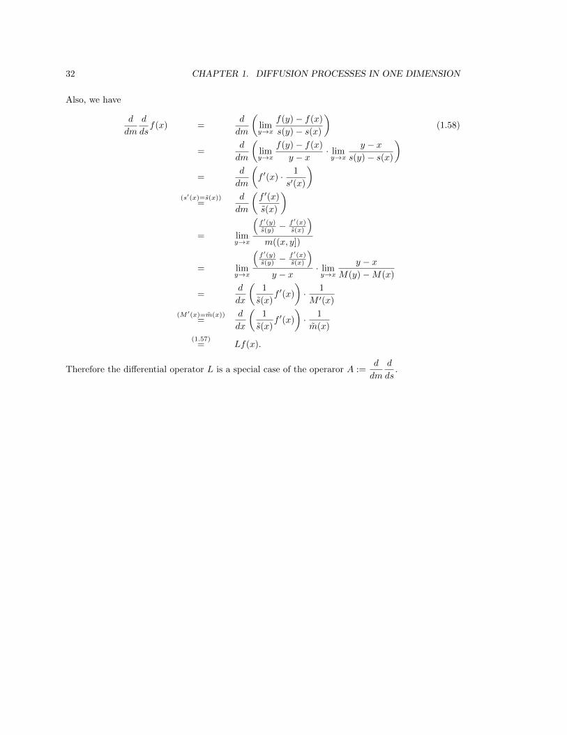
Also, we have

d

dm

d

dsf(x) =

d

dm

(limy→x

f(y)− f(x)

s(y)− s(x)

)(1.58)

=d

dm

(limy→x

f(y)− f(x)

y − x· limy→x

y − xs(y)− s(x)

)=

d

dm

(f ′(x) · 1

s′(x)

)(s′(x)=s(x))

=d

dm

(f ′(x)

s(x)

)

= limy→x

(f ′(y)s(y) −

f ′(x)s(x)

)m((x, y])

= limy→x

(f ′(y)s(y) −

f ′(x)s(x)

)y − x

· limy→x

y − xM(y)−M(x)

=d

dx

(1

s(x)f ′(x)

)· 1

M ′(x)

(M ′(x)=m(x))=

d

dx

(1

s(x)f ′(x)

)· 1

m(x)

(1.57)= Lf(x).

Therefore the differential operator L is a special case of the operaror A :=d

dm

d

ds.

Chapter 2

Orthogonal polynomials in onedimension

2.1 Orthogonal polynomials

In this section we will look at some basic concepts on orthogonal polynomials, and some importanttheorems in relation with this topic.

Definition 2.1.1. Let (a, b) ⊆ R and w : (a, b) → R a positive function. We say that a set ofpolynomials p0, p1, ... (with pn of degree n) is orthogonal respect to w, if

〈pn, pm〉 := 〈pn, pm〉w :=

∫ b

a

pn(x)pm(x) w(x)dx = dnδnm,

where dn 6= 0, and δnm denotes the Kronecker delta, that is, δnm = 0 if n 6= m, and δnm = 1 ifn = m. If, in addition, dn = 1 we say that the polynomials are orthonormal.

Theorem 2.1.2. Let w : (a, b) → R be a positive function. Then there exists a sequence oforthogonal polynomials pn with respect to w such that 〈pn, pm〉w = dnδnm.

Proof. Use the Gram-Schmidt process in the sequence of polynomials pn(x) := xn with the inner

product 〈f, g〉 :=∫ baf(x)g(x)w(x)dx.

Theorem 2.1.3. Let pn be a sequence of orthogonal polynomials (of degree n) with respect to w.Then 〈pn, q〉w = 0 for any polynomial q of degree m < n; that is, the polinomial pn is orthogonalto any polynomial of degree less that n.

Proof. Note that any polynomial of degree m, where m < n can be written as a linear combi-nation of the polynomials p0, p1, ..., pm. Let q be a polynomial of degree m. Then there exist

α1, α2, ..., αm such that q =

m∑k=0

αkpk. Then 〈pn, q〉w =m∑k=0

αk〈pn, pk〉w = 0.

33

34 CHAPTER 2. ORTHOGONAL POLYNOMIALS IN ONE DIMENSION

Theorem 2.1.4. If pn and qn are two orthogonal polynomials (of degree n) with respect to w, thenthere exists λ 6= 0 such that pn = λqn.

Proof. Pick λ such that the degree of pn − λqn is n − 1. By the previous theorem we know that〈pn, pn − λqn〉w = 0 and 〈qn, pn − λqn〉w = 0. This implies that 〈pn, pn〉w = λ〈pn, qn〉w and〈qn, pn〉w = λ〈qn, qn〉w.

Then ‖pn − λqn‖2 = 〈pn − λqn, pn − λqn〉w = 0, therefore pn − λqn = 0.

Note 1: In this chapter, A always represents a polynomial of degree at most 2 and B a polynomialof degree at most 1. This is so is because if A or B do not satisfy this condition, then there does notexist a polynomial P that is solution of the differential equation A(x)P ′′(x)+B(x)P ′(x)+λP (x) = 0(see e.g. [12]). Also, w : (a, b)→ R is a positive function.

Theorem 2.1.5. Let A, B and w be defined as in Note 1. Assume that

d

dx(A(x)w(x)) = B(x)w(x).

Thenlimx→a+

xnA(x)w(x) = 0, n = 0, 1, 2... (2.1)

Proof. We have that (xnA(x)w(x))′ = xn(A(x)w(x))′ + nxn−1A(x)w(x), n = 0, 1, 2..., and byassumption we know that (A(x)w(x))′ = B(x)w(x), then

(xnA(x)w(x))′ = xnB(x)w(x) + nxn−1A(x)w(x).

By integrating both sides we obtain

xnA(x)w(x) =

∫ x

a

[snB(s)w(s) + nsn−1A(s)w(s)]ds.

Since snB(s)w(s) + nsn−1A(s)w(s) is continuous, the integral is continuous. Therefore we arriveto lim

x→a+xnA(x)w(x) = 0.

Similarly we obtain thatlimx→b−

xnA(x)w(x) = 0, n = 0, 1, 2... (2.2)

2.2 The derivative of orthogonal polynomials

Theorem 2.2.1. Let A and B be polynomials as in Note 1, and let w : (a, b) → R be a pos-itive function. Let qn be a sequence of orthogonal polynomials with respect to w, such that(A(x)w(x))′ = B(x)w(x). Then q′n is a sequence of orthogonal polynomials with respect tow1 := Aw.

Proof. Let n > m, and define φ(x) := xm−1B(x). We know that

〈φ, qn〉w =

∫ b

a

xm−1B(x)qn(x)w(x)dx = 0, (2.3)

2.3. A DIFFERENTIAL EQUATION FOR THE ORTHOGONAL POLYNOMIALS 35

because the degree of xm−1B(x) is less than n.

On the other hand, by using (A(x)w(x))′ = B(x)w(x)

〈φ, qn〉w =

∫ b

a

xm−1qn(x)[B(x)w(x)]dx =

∫ b

a

xm−1qn(x)(A(x)w(x))′dx.

Using (2.3), integration by parts and Theorem 2.1.5 we arrive to

0 = 〈φ, qn〉w = −(m− 1)

∫ b

a

xm−2A(x)qn(x)w(x)dx−∫ b

a

xm−1A(x)q′n(x)w(x)dx.

Also, we know that ∫ b

a

xm−2A(x)qn(x)w(x)dx = 0,

because the degree of xm−2A(x) is less than n.

Hence ∫ b

a

xm−1q′n(x)[A(x)w(x)]dx = 0.

Therefore, the sequence q′n is orthogonal with respect to w1 = Aw.

Corollary 2.2.2. Let A and B as in the note 1. Let qn be a sequence of orthogonal polynomialswith respect to w, such that they satisfy the equation (A(x)w(x))′ = B(x)w(x). Then the sequence

q(m)n of polynomials is orthogonal with respect to wm := Amw.

Also (A(x)wm(x))′ = Bm(x)wm(x), with Bm(x) = A′(x)m+B(x).

Proof. One can repeat the process in the proof of Theorem 2.2.1.

2.3 A differential equation for the orthogonal polynomials

Theorem 2.3.1. Let A, B and w as in note 1, and such that (A(x)w(x))′ = B(x)w(x). Then theset of orthogonal polynomials with respect to w are solution of the differential equation

A(x)f ′′(x) +B(x)f ′(x) + λnf(x) = 0,

where λn = −n[ (n−1)2 A′′ +B′].

Proof. By Theorem 2.2.1 we know that q′n is a sequence of orthogonal polynomials with respect toAw. Also, abusing of the notation we have

〈q′n(x), xm−1〉Aw = 0 if m < n. (2.4)

Using integration by parts, (2.1) and (2.2) we obtain

0 = 〈q′n(x), xm−1〉Aw =−1

m

∫ b

a

xm[A(x)q′n(x)w(x)]′dx. (2.5)


Note that

[A(x)q′n(x)w(x)]′ = A′(x)q′n(x)w(x) +A(x)q′′n(x)w(x) +A(x)q′n(x)w′(x),

but

A′(x)q′n(x)w(x) +A(x)q′n(x)w′(x) = q′n(x)[A′(x)w(x) +A(x)(x)w′(x)] = q′n(x)B(x)w(x).

Then[A(x)q′n(x)w(x)]′ = A(x)q′′n(x)w(x) + q′n(x)B(x)w(x),

And by (2.5)

0 =

∫ b

a

xm[A(x)q′′n(x) + q′n(x)B(x)]w(x)dx.

This says that the polynomial A(x)q′′n(x) + q′n(x)B(x) of degree n is orthogonal to the polynomialsof degree m with respect to w, with m < n. Therefore by Theorem 2.1.4 there exists −λn 6= 0such that

A(x)q′′n(x) +B(x)q′n(x) = −λnqn(x).

Then, comparing coefficients in

A(x)q′′n(x) +B(x)q′n(x) + λnqn(x) = 0, (2.6)

we obtain λn = −n[ (n−1)2 A′′ +B′].

2.4 Classical orthogonal polynomials

Some classical orthogonal polynomials are specified in the following table:

Polynomial Interval A(x) w(x) B(x)Jacobi (−1, 1) 1− x2 (1− x)α(1 + x)β β − α− (α+ β + 2)x

Laguerre (0,∞) x xαe−x α+ 1− xHermite (−∞,∞) 1 e−x

2 −2x

By Theorem 2.3.1 we know that the Jacobi polynomials are solution of the differential equation

(1− x2)J ′′n(x) + [β − α− (α+ β + 2)x]J ′n(x) + n(n+ α+ β + 1)Jn(x) = 0. (2.7)

The Laguerre polynomials are solution of

xL′′n(x) + [α+ 1− x]L′n(x) + nLn(x) = 0. (2.8)

The Hermite polynomials are solution of

H ′′n(x)− 2xH ′n(x) + 2nHn(x) = 0. (2.9)

2.5. THE FORMULA OF RODRIGUES TYPE 37

Note that the general equation is of the form

A(x)p′′n(x) +B(x)p′n(x) = −λnpn(x),

and we see that the orthogonal polynomials are eigenfunctions of the operator Lf := Af ′′ + Bf ′

associated with the eigenvalues given by the Theorem 2.3.1.

2.5 The formula of Rodrigues type

The solutions of the equations (2.7), (2.8) and (2.9) can be expressed compactly using the formulaof Rodrigues type which is derived using the following lemma.

Lemma 2.5.1. For m = 0, 1, 2..., the sequence of orthogonal polynomials q(m)n satisfies

d

dx

(A(x)wm(x)

d

dx(q(m)n (x))

)= λn,mwm(x)q(m)

n (x), n = 0, 1, 2..., (2.10)

where λn,m = (n−m)(

12 (n+m− 1)A′′(0) +B′(0)

)and wm(x) is as in Corollary 2.2.2.

Proof. Note that

d

dx

(A(x)wm(x)

d

dx(q(m)n (x))

)= wm(x)[Bm(x)q(m+1)

n (x) +A(x)q(m+2)n (x)]

= wm(x)[Bm(x)(q(m)n (x))′ +A(x)(q(m)

n (x))′].

because (A(x)wm(x))′ = Bm(x)wm(x) by Corollary 2.2.2. Also, again by Corollary 2.2.2 and

Theorem 2.3.1, there exist λn,m such that the sequence of orthogonal polynomials q(m)n are solution

ofA(x)(q(m)

n (x))′′ +Bm(x)(q(m)n (x))′ = λn,mq

(m)n (x). (2.11)

Thend

dx

(A(x)wm(x)

d

dx(q(m)n (x))

)= wm(x)λn,mq

(m)n (x).

Comparing coefficients in the equation (2.11) we obtain

λn,m = (n−m)

(1

2(n+m− 1)A′′(0) +B′(0)

).

Theorem 2.5.2 (Formula of Rodrigues type ). The orthogonal polynomials qn with respect to wcan be written in the form

qn(x) =cnw(x)

dn

dxn(An(x)w(x)) , (2.12)

where cn is a constant.


Proof. We apply Lemma 2.5.1 several times. If m = 0 in (2.10), we have

(A(x)w(x)q′n(x))′ = λn,0w(x)qn(x). (2.13)

Note that w1(x)q′n(x) = A(x)w(x)q′n(x). Then by substituting in (2.13) we obtain

λn,0w(x)qn(x) = (w1(x)q′n(x))′ =(λn,1w1(x)q′n(x))′

λn,1. (2.14)

Applying again (2.10) in (2.14) with m = 1 we obtain

(λn,1w1(x)q′n(x))′

λn,1=

(A(x)w1(x)q′′n(x))′′

λn,1.

Now, since w2(x) = A2(x)w(x) = A(x)w1(x), by applying again (2.10) to the above equation wearrive at

λn,0w(x)qn(x) =(w2(x)q′′n(x))′′

λn,1=

(λn,2w2(x)q′′n(x))′′

λn,2λn,1=

(A(x)w2(x)q′′′n (x))′′′

λn,2λn,1.

Continuing with this process we obtain

λn,0w(x)qn(x) =(A(x)wn−1(x)q

(n)n (x))(n)

λn,n−1 · · · λn,1. (2.15)

Note that q(n)n is constant. Then from (2.15) we arrive to

qn(x) =cnw(x)

(A(x)wn−1(x))(n), (2.16)

where cn =q

(n)n (x)

λn,n−1 · · · λn,1λn,0. Since wn−1(x) = An−1(x)w(x), substituting in (2.16) we obtain

the result.

2.6 Completeness of the orthogonal polynomials

Other important result that we will prove is that the orthogonal polynomials with respect to the

function w form a base of L2((a, b), w(x)dx) :=

f :

∫ b

a

f2(x)w(x)dx <∞

. For this purpose, we

use the Fourier transform.

2.6. COMPLETENESS OF THE ORTHOGONAL POLYNOMIALS 39

2.6.1 Hermite polynomials

Note that the space generated by the Hermite polynomials coincides with the space generated bythe polynomials 1, x, x2, x3, .... Let E be the closure of the space generated by these monomials.

Suppose that E 6= L2(R, e−x2

dx). Then there exists f ∈ L2(R, e−x2

dx)−E such that f−PE(f) 6= 0,where PE is the orthogonal projection on E.

Then, by definition of PE , we have that for all e ∈ E

〈e, f − PE(f)〉w = 0, (2.17)

In particular for e := xn, for all n = 0, 1, 2...

On the other hand, let g ∈ L2(R, e−x2

dx). If 〈xn, g〉w = 0 for all n, then the function G defined by

G(z) :=

∫ ∞−∞

ezxg(x)e−x2

dx,

is 0 for every z, because

G(z) =

∫ ∞−∞

ezxg(x)e−x2

dx =

∞∑n=0

zn

n!

∫ ∞−∞

xng(x)e−x2

dx = 0.

If we pick z = it, we have

∫ ∞−∞

eitxg(x)e−x2

dx = 0. This implies that the Fourier transform

of g(x)e−x2

is 0. Then g(x)e−x2

= 0 is the function 0 in L2(R, e−x2

dx), and thus so is g. Inparticular, this holds for g := f − PE(f), which implies that PE(f) = f . This contradicts the factthat f − PE(f) 6= 0.

Therefore the Hermite polynomials form a orthogonal basis for the space L2(R, e−x2

dx).

2.6.2 Jacobi polynomials

We use the same idea of the previous proof. Note that the space generated by the Jacobi polyno-mials equals the space generated by the polynomials 1, x, x2, x3, .... Let E be the closure of thespace generated by these monomials.

Suppose that E 6= L2((−1, 1), (1− x)α(1 + x)βdx). Then there exists f ∈ L2(R, e−x2

dx)−E suchthat f − PE(f) 6= 0, where PE is the orthogonal projection on E.

Then, by definition of PE , we have that for all e ∈ E

〈e, f − PE(f)〉w = 0, (2.18)

In particular for e := xn, for all n = 0, 1, 2...

On the other hand, let g ∈ L2((−1, 1), (1 − x)α(1 + x)βdx). If 〈xn, g〉w = 0 for all n, then thefunction G defined by

G(z) :=

∫ 1

−1

ezxg(x)(1− x)α(1 + x)βdx,


is 0 for every z, because

G(z) =

∫ 1

−1

ezxg(x)(1− x)α(1 + x)βdx =

∞∑n=0

zn

n!

∫ 1

−1

xng(x)(1− x)α(1 + x)βdx = 0.

If we pick z = it, we have

∫ ∞−∞

eitxg(x)1(x)(−1,1)(1−x)α(1+x)βdx = 0. This implies that the Fourier

transform of g(x)1(x)(−1,1)(1 − x)α(1 + x)β is 0. Then g(x)1

(x)(−1,1)(1 − x)α(1 + x)β is the function 0

in L2((−1, 1), (1 − x)α(1 + x)βdx), and thus so is g. In particular, this holds for g := f − PE(f),which implies that PE(f) = f . This contradicts the fact that f − PE(f) 6= 0.

Therefore the Jacobi polynomials form an orthogonal basis for the space L2((−1, 1), (1− x)α(1 +x)βdx).

Note: The proof that the Laguerre polynomials form an orthogonal basis for the Hilbert spaceL2((0,∞), xαe−xdx) is similar.

2.7 Example: Hermite polynomials

2.7.1 The three terms recurrence relation

The Hermite polynomials can be defined applying the Rodrigues formula, with A(x) := 1, B(x) :=

−2x, and w(x) := e−x2

. Then one arrives at

Hn(x) := (−1)nex2 dn

dxne−x

2

. (2.19)

By induction it is easy to check that

dn+1

dxn+1e−x

2

= −2xdn

dxne−x

2

− 2ndn−1

dxn−1e−x

2

. (2.20)

Multiplying both sides of (2.20) by (−1)nex2

we arrive at the following recurrence relation for theHermite polynomials:

Hn+1(x) = 2xHn(x)− 2nHn−1(x). (2.21)

On the other hand, it is also easy to verify

H ′n(x) = 2xHn(x)−Hn+1(x), (2.22)

and also that

H ′n(x) = 2nHn−1(x). (2.23)

2.7. EXAMPLE: HERMITE POLYNOMIALS 41

2.7.2 Orthogonality of the Hermite polynomials

The Hermite polynomials are orthogonal with respect to the function w(x) = e−x2

. We will showthat ∫ ∞

−∞Hn(x)Hm(x)e−x

2

dx = 0 if n 6= m.

Suppose that n > m. Then using integration by parts m times we have∫ ∞−∞

Hn(x)Hm(x)e−x2

dx = (−1)n∫ ∞−∞

Hm(x)dn

dxne−x

2

dx

= (−1)n+1

∫ ∞−∞

H ′m(x)dn−1

dxn−1e−x

2

dx

= (−1)n+2

∫ ∞−∞

H ′′m(x)dn−2

dxn−2e−x

2

dx

...

= (−1)n+m

∫ ∞−∞

H(m)m (x)

dn−m

dxn−me−x

2

dx

= (−1)n+mH(m)m (x)

∫ ∞−∞

dn−m

dxn−me−x

2

dx

= (−1)n+mH(m)m (x)

dn−m−1

dxn−m−1e−x

2

∣∣∣∣∞−∞

= 0. (2.24)

Now, we will show that ∫ ∞−∞

(Hn(x))2e−x2

dx = n!2n√π.

By (2.24), if n = m we arrive at∫ ∞−∞

(Hn(x))2e−x2

dx =

∫ ∞−∞

H(n)n (x)e−x

2

dx. (2.25)

By (2.23) we have that H ′n(x) = 2nHn−1(x), and differentiating both side of this equality weobtain H ′′n(x) = 2n · 2(n− 1)Hn−2(x). Applying this process n times we arrive at

H(n)n (x) = 2n · 2(n− 1) · · · 2(1)H0(x).

Since H0(x) = 1, then H(n)n (x) = n!2n. Substituting in (2.25) we obtain∫ ∞−∞

(Hn(x))2e−x2

dx = n!2n∫ ∞−∞

e−x2

dx = n!2n√π.

Therefore the Hermite polynomials are orthogonal on L2(R, e−x2

dx).

Chapter 3

Diffusions and orthogonalpolynomials

In this chapter we characterize the density probability function of the diffusion processes: Jacobi,Ornstein-Uhlenbeck and Cox-Ingersoll-Ross. We do so by using orthogonal polynomials. At theend we give an example of a diffusion that does not fit as a classical example: the Brox diffusion.

3.1 The Ornstein-Uhlenbeck process

The Ornstein-Uhlenbeck process is solution of the stochastic differential equation

dXt = −Xtdt+ dBt. (3.1)

It is known that the infinitesimal operator associated with this process is

Lf(x) :=1

2f ′′(x)− xf ′(x). (3.2)

Note that the Hermite polynomials are solution of LHn(x) = −nHn(x). Remember that the do-main of L are the functions f such that f and Lf vanish at infinity. Then the Hermite polynomialsdo not belong to the domain of L.

But if we consider the space L2(R, e−x2

dx) :=

f :

∫ ∞−∞

f2(x)e−x2

dx <∞

, then the Hermite

polynomials are functions vanishing at infinity on L2(R, e−x2

dx). Therefore on L2(R, e−x2

dx) itmakes sense to consider LHn(x) = −nHn(x).

We known that the Hermite polynomials form an orthogonal basis of the Hilbert space L2(R, e−x2

dx)

with the inner product given by 〈f, g〉 :=

∫ ∞−∞

f(x)g(x)e−x2

dx. Also these polynomials satisfy∫ ∞−∞

H2n(x)e−x

2

dx = n!2n√π. See chapter 2.

Then the polynomials Hn√n!2n

√π

form an orthonormal basis for the Hilbert space L2(R, e−x2

dx) and

they satisfy L

(Hn(x)√n!2n

√π

)= −n

(Hn(x)√n!2n

√π

).

43

44 CHAPTER 3. DIFFUSIONS AND ORTHOGONAL POLYNOMIALS

We want to express the transition function of the Ornstein-Uhlenbeck process in terms of theHermite polynomials. To this end, note that C0(R) ⊆ L2(R, e−x2

dx), and so any f ∈ C0(R) can

be written as a linear combination of the orthonormal basis of L2(R, e−x2

dx). Therefore we arriveto

f =

∞∑n=0

〈f, φn〉φn, (3.3)

where φn :=Hn√n!2n√π

, and 〈f, φn〉 :=

∫ ∞−∞

f(x)φn(x)e−x2

dx.

Since φn is an eigenfunction of L corresponding to the eigenvalue λn := −n, i.e. Lφn = −nφn,then one can check that uf (t, x) := e−nt〈f, φn〉φn(x) solves the equation

∂uf (t, x)

∂t= Luf (t, x), u(0, x) = 〈f, φn〉φn(x). (3.4)

If uf (t, x) is a superposition of such functions, i.e. uf (t, x) :=

∞∑n=0

e−nt〈f, φn〉φn(x), then uf (t, x)

solves the equation

∂uf (t, x)

∂t= Luf (t, x), uf (0, x) = f(x). (3.5)

On the other hand, applying the properties of semigroups we obtain that Ptf(x) also satisfies theequation (3.5). Hence Ptf(x) = uf (t, x), because the solution is unique. (See e.g [9, p.500]).

Since Ptf(x) := E(f(Xt)|X0 = x) =

∫ ∞−∞

f(y)p(t, x, dy), using the dominated convergence theorem

we arrive at ∫ ∞−∞

f(y)p(t, x, dy) =

∞∑n=0

e−nt〈f, φn〉φn(x)

=

∞∑n=0

e−nt(∫ ∞−∞

f(y)φn(y)e−y2

dy

)φn(x)

=

∫ ∞−∞

f(y)

( ∞∑n=0

e−ntφn(y)φn(x)e−y2

)dy.

Then p(t, x, dy) has a density p(t, x, y), and it is given by

p(t, x, y) = e−y2∞∑n=0

e−nt

n!2n√πHn(y)Hn(x). (3.6)

These same arguments can be applied to diffusions where other orthonormal polynomials areeigenfunctions of the infinitesimal operator. This can be done by taking into consideration asuitable Hilbert space where the polynomials form an orthonormal basis.

3.2. THE COX-INGERSOLL-ROSS PROCESS 45

3.2 The Cox-Ingersoll-Ross process

The Cox-Ingersoll-Ross process is solution of the stochastic differential equation

dXt = (1−Xt)dt+√

2XtdBt.

The infinitesimal operator associated with this process is

Lf(x) := xf ′′(x) + (1− x)f ′(x).

Also, the Laguerre polynomials Ln, n = 0, 1, 2... in (2.8), are eigenfunctions of L associated withthe eigenvalues λn := −n.

If we consider the space L2((0,∞), e−xdx), with the inner product 〈f, g〉 :=

∫ ∞0

f(x)g(x)e−xdx,

then the Laguerre polynomials form an orthogonal basis, and multiplying by a suitable constantCn we obtain that ϕn := CnLn, n = 0, 1, 2..., form an orthonormal basis of the Hilbert spaceL2((0,∞), e−xdx).

Applying the same arguments used in section 3.1, we obtain that the Cox-Ingersoll-Ross processhas a density function, which is given by

p(t, x, y) = e−y∞∑n=0

e−ntC2nLn(y)Ln(x).

3.3 The Jacobi process

The Jacobi process is solution of the stochastic differential equation

dXt = [(β − α)− (α+ β + 2)Xt]dt+√

2(1−X2t ) dBt.

In this case, the associated infinitesimal operator is

Lf(x) := (1− x2)f ′′(x) + [(β − α)− (α+ β + 2)x]f ′(x).

And the eigenfunctions of L are the Jacobi polynomials Jn, n = 0, 1, 2... in (2.7), associated withthe eigenvalues λn := −n(n+ α+ β + 1).

Consider L2((−1, 1), (1− x)α(1 + x)βdx

), with 〈f, g〉 :=

∫ 1

−1

f(x)g(x)(1 − x)α(1 + x)βdx. Then

for suitable constants Kn, the functions ψn := KnJn, n = 0, 1, 2... form an orthonormal basis ofthe Hilbert space L2

((−1, 1), (1− x)α(1 + x)βdx

).

Now, apply the same arguments as in the section 3.1, we obtain that the Jacobi process has adensity function given by

p(t, x, y) = (1− y)α(1 + y)β∞∑n=0

e−n(n+α+β+1)tK2nJn(y)Jn(x).


3.4 The Brox process

As part of the motivation of this thesis, we will show an example of one diffusion whose associated

infinitesimal operator is not of the classical form Lf(x) := µ(x)f ′(x)+1

2σ2(x)f ′′(x). This diffusion

is called the Brox process (see e.g. [11]).

Consider informally the equation

dXt = −1

2W ′(Xt)dt+ dBt, (3.7)

where B := Bt : t ≥ 0 is the standard Brownian motion, and W := W (x) : x ∈ R is a two sidedBrownian motion, and they are both independent of each other. Here W ′ denotes the derivativeof W , sometimes called the white noise.

When leaving fixed a trajectory of W , the equation (3.7) can be interpreted as a stochastic differ-ential equation. This way of thinking corresponds to considering the process X := Xt : t ≥ 0associated with the infinitesimal operator

Lf(x) :=1

2eW (x) d

dx

(e−W (x) df(x)

dx

). (3.8)

This corresponds to considering the scale function

s(x) :=

∫ x

0

eW (y)dy, (3.9)

and the speed measure

m(A) :=

∫A

2e−W (y)dy, for Borel sets A ⊆ R. (3.10)

Let us check so:

d

dm

d

dsf(x) =

d

dm

(limh→0

f(x+ h)− f(x)

s(x+ h)− s(x)

)=

d

dm

(limh→0

f(x+ h)− f(x)

h· limh→0

11h

∫ x+h

xeW (y)dy

)

=d

dm

(e−W (x)f ′(x)

)= lim

h→0

f ′(x+ h)e−W (x+h) − f ′(x)e−W (x)

m((x, x+ h])

= limh→0

f ′(x+ h)e−W (x+h) − f ′(x)e−W (x)∫ x+h

x2e−W (y)dy

= limh→0

f ′(x+ h)e−W (x+h) − f ′(x)e−W (x)

h· limh→0

11h

∫ x+h

x2e−W (y)dy

=d

dx

(e−W (x) d

dxf(x)

)· e

W (x)

2

= Lf(x). (3.11)

3.4. THE BROX PROCESS 47

Then one considers rigourously the operatord

dm

d

dsf , where s is the scale function defined in (3.9),

and m is the speed measure defined in (3.10). We want to see that the process X associated withthis operator is a diffusion, when leaving fixed W .

To this end, we use a result of K. Ito and H.P.McKean (see e.g. [5, p.165]), where we can reconstructa process Y in natural scale through the speed measure mY and the local time. The procedure isdone in the following way. Observe that

Xt = BT−1t, (3.12)

where

Tt :=

∫ ∞−∞

Lt(x)mY (dx), (3.13)

and Lt(y) is the so-called local time (see e.g. [7, p.32]), which can be calculated as

Lt(y) := limε→0

1

2ε

∫ t

0

1x−ε<Bs<x+εds. (3.14)

In our case, the process X is not in natural scale, but the new process Yt := s(Xt) is in naturalscale [3]. Now, by applying the Ito formula (see e.g. [4, p.149]), we find that s(Xt) satisfies theequation

ds(Xt) = eW (Xt)dBt = eW (s−1(s(Xt)))dBt.

ThusdYt = 0dt+ eW (s−1(Yt))dBt. (3.15)

Leaving fixed a trajectory of W , the equation (3.15) can be interpreted as a stochastic differentialequation. Then the process Y is associated with the infinitesimal operator

LY f(x) = eW (s−1(x))f ′′(x). (3.16)

By the formula (1.56) and (3.16), we obtain that the speed measure associated with the processYt is

mY (A) =

∫A

2e−W (s−1(x))dx,

for any Borel set A.

Then applying the reconstruction of K. Ito and and H.P.McKean one has

s(Xt) = BT−1t,

with Tt as in ( 3.13) .

But BT−1t

is a diffusion (see e.g. [6, p.277]), and so s(Xt) is a diffusion. Hence since s is continuous

and strictly increasing, Xt = s−1(BT−1t

) is a diffusion process for each trajectory W. One could

write XW to emphasize that the diffusion process X is conditioned to W .

Let us define rigourously the process X when it is not conditioned to W . We leave fixed a trajectoryW , then we denote by PW the corresponding probability measure of XW over C([0,∞)), and if µ


is the probability measure over C(R) associated to the Brownian motion W : Ω→ C(R), then bythe law of total probability we obtain the formula for the corresponding probability measure of Xwithout fixing W :

P (C) =

∫Ω

PW (ω)(C)µ(dω),

for any measurable set C in C([0,∞)).

Bibliography

[1] B. Oksendal. (2003). Stochastic Differential Equations. Springer-Verlag.

[2] C. Tudor. (2002). Procesos Estocasticos. Sociedad Matematica Mexicana.

[3] D. Revuz, M. Yor. (1999). Continuous Martingales and Brownian Motion. Springer-Verlag.

[4] F.C. Klebaner. (2005). Introduction to Stochastic Calculus with Applications. Imperial Col-lege Press.

[5] K. Ito, H.P. Mckean. (1965). Diffusion Processes and their Sample Paths. Springer-Verlag

[6] L.Rogers, D. Williams. (1987). Diffusions, Markov Processes, and Martingales. Wiley.

[7] M.B. Marcus, J. Rosen. (2006). Markov Processes, Gaussian Processes, and Local Times.Cambridge University Press.

[8] P. Mandl. (1968). Analytical Treatment of one Dimensional Markov Processes. Academia,Publishing House of the Czechoslovak Academy of Sciences.

[9] R.N. Bhattacharya, E. C. Waymire. (1990). Stochastic Processes with Applications. Wiley.

[10] S. Karlin, H.M. Taylor. (1981). A Second Course in Sthochastic Processes. Academic Press.

[11] Th. Brox. (1986). A one dimensional diffusion process in a Wiener medium. The Annals ofProbability, Vol.14. No.4, 1206-1218.

[12] T.S. Chihara (1978). An Introduction to Orthogonal Polynomials. Gordon and Breach.

[13] W. Schoutens. (2000). Stochastic Processes and Orthogonal Polynomials. Springer-Verlag.

49

centro de investigacion y de estudios avanzados … · dedicado a mi familia, a mi pap a francisco...

Documents