XLIX Reunión AnualNoviembre de 2014

ISSN 1852-0022ISBN 978-987-28590-2-2

A CENTURY OF NOMINAL HISTORY IN ARGENTINA: MONETARY INSTABILITY AND NON-NEUTRALITIES

Basco EmilianoBurdisso TamaraCorso EduardoD'Amato LauraGrillo FedericoKatz Sebastián

ANALES | ASOCIACION ARGENTINA DE ECONOMIA POLITICA

1

A Century of nominal history in Argentina: monetary instability and non-neutralities*† Emiliano Basco (UBA-UNLaM-BCRA ) Tamara Burdisso (UBA-BCRA) Eduardo Corso (UBA-BCRA ) Laura D´Amato (UBA-BCRA ) Federico Grillo (BCRA) Sebastian Katz (UBA-UdeSA-BCRA)

First Draft August, 2014

Abstract We use a bivariate ARIMA model to test the neutrality hypotheses for Argentina over the period 1900-2012. We find that over the whole period permanent shocks to monetary aggregates have a more than proportional on prices and a negative permanent impact on real GDP. To investigate if these findings are related to a particular regime we test for structural breaks using Bai-Perron methodology. We verify that more than proportional price responses and “negative long-run non-neutrality” only appear in price instability environments. This negative non-neutrality could reflect the presence of disruptive mechanisms identify in the literature in high inflation environments. JEL classification: C31, C41, C51, C22, C51. Keywords: Money, prices, real GDP, neutrality, unit roots, structural breaks, Argentina.

* ebasco@gmail.com; tamaraburdisso@gmail.com;eacorso@yahoo.com; laura.damato@gmail.com; fedogrillo@gmail.com; katzberm@gmail.com The opinions expressed in this paper are of the authors and do not necessarily represent those of the BCRA. † A preliminary version of this paper was presented at VII Congreso Internacional de Economía y Gestión “Econ 2013” organized by Facultad de Ciencias Económicas, UBA, in the “Cien años de economía y sociedad en la Argentina 1913 – 2013” session. We would like to thanks Prebisch Library staff and Tornquist Library staff, and specially Mariano Iglesias, for their invaluable assistance in the search for economic history literature and data.

2

Resumen Utilizamos un modelo ARIMA bivariado parra testear las hipótesis de neutralidad de Argentina durante el período 1900-2012. Encontramos que para todo el período shocks permanentes a los agregados monetarios tienen un impacto más que proporcional en los precios y uno negativo en el PIB real. Para investigar si estos hallazgos se deben a algún régimen nominal en particular testeamos la presencia de quiebres estructurales usando la metodología de Bai-Perron. Verificamos la respuesta más que proporcional de los precios al dinero y las no-neutralidades negativas sólo aparecen en entornos de inestabilidad de precios. Esta no-neutralidad negativa podría reflejar la presencia de mecanismos disruptivos identificados por la literatura en entornos de alta inflación. Clasificación JEL: C31, C41, C51, C22, C51. Palabras Clave: dinero, precios, PIB real, neutralidad, raíces unitarias, quiebre estructural, Argentina.

3

I. Introduction

“South Americans… are always in trouble about their currency. Either it is too good for home use, or, as frequently happens, it is too bad for foreign exchange. Generally they have too much of it, but their own idea is that they never have enough… the Argentines alter their currency almost as frequently as they change their presidents… No people in the world take a keener interest in currency experiments than the Argentines.” W. R. Lawson in The Bankers Magazine of 1899, quoted in Alec Ford (1962).

Typically considered a disputed and controversial subject, there are no many consensual propositions in macroeconomics. The idea that in the long run nominal variables behave in a neutral (or “superneutral”) way can probably be one of the few of them. A member of a more general family of “irrelevance hypothesis” –that includes, besides others, Fisher’s parity, the neutrality of exchange rate regimes, PPP, Modigliani-Miller theorem and its associated lemmas like the Ricardian equivalence- neutrality of money is probably the best known of these propositions. Following this notion, permanent changes in monetary aggregates –in its levels or its rates of growth- should translate in proportional variations of absolute prices –or in the general inflation rate- without affecting relative prices and the associated real quantities. A broad body of evidence tends to confirm this theoretical assumption. In fact, one of the more robust empirical regularities in the literature is the existence of a strong positive correlation between money and prices in the long run and that this relationship is close to proportional (Lucas, 1980; McCandless and Weber, 1995). Many papers, however, suggest that this relationship could be contingent to the prevailing macroeconomic regime and that in low inflation contexts proportionality can weaken (Sargent and Surico, 2011). Basco, D´Amato and Garegnani (2009) and Bozzoli and della Paolera (2014) verify this stylized fact for some periods in Argentina. At the same time, in line with neutrality hypothesis, the evidence tends to indicate the that there is no long run correlation between monetary evolution and the behavior of real GDP. However, this finding is not as robust as the previous one (Walsh, 2003). McCandless et al. (1995) found that there is no correlation between money growth and real GDP growth for a large set of countries but positive one for a subsample of OECD over the period 1960-1990. This is not the only empirical mismatch of the empirical evidence with the orthogonality assumption about nominal and real developments. More relevant is the fact that this theoretical assumption contrasts with abundant empirical evidence that shows that countries experiencing macro instability –and high inflation in particular- tend to exhibit a notably worst real performance than countries functioning in a more stable nominal environment (see, among others, Barro 1995, 1996). Long run “negative” non-neutralities of this kind are not easy to accommodate for standard monetary theory (Heymann and Leijonhufvud, 1995). As Tobin (1992) says, “…theory puts the burden of the proof on anyone who contends that money and monetary inflations or deflations” can have serious consequences for economic activity and general well being. Strictly following neutrality, the consequences of monetary policies are supposed to be irrelevant in the long run because, in equilibrium, a perfectly anticipated inflation has no real effects, except for the distortionary effects of the inflation tax.

4

Of course, in the short-run inflationary surprises can have positive real effects on output if agents make expectational mistakes. These effects are however, transitory and disappear once the monetary authority abuses of inflationary surprises. Moreover, this abuse in using monetary policy to stimulate the economy could also lead to a lack of credibility in stabilization policies, generating a higher sacrifice ratio. If this is all, pure economic theory does not seem to provide enough compelling reasons for the generalized dislike that people feel against inflation (Barro and Fischer, 1976). This is not, however, what the empirical evidence on inflationary regimes shows. Through many and diverse channels, nominal instability has huge costs on the real performance of economies and strong negative effects on welfare. Money is an institution that has evolved to facilitate trade and allows society to develop complex patterns of division of labor. By severely impairing economic calculation, the bad functioning of monetary institutions in high inflation makes very difficult to coordinate economic activities. Nominal uncertainty leads agents to waste resources and to dedicate unnecessary efforts to the process of exchange. At the same time, in an uncertain context the possibility of experiencing huge capital losses and arbitrary redistributions of wealth leads agents to modify their microeconomic behavior. Strong “flexibility preference” in the sense of Hicks (1974) and the drastic shortening of relevant time horizons are two basic adaptive features of these episodes (Fanelli and Frenkel, 1995). Credit disintermediation and the negative reward of long run maturity activities like investment and innovation seriously affect the possibility of economic growth. It is through these various effects of “economic disorganization” that monetary instability could generate the “negative” long run non-neutralities that explain the public’s –and economist’s- dislike for inflation. Proliferation of monetary disorder episodes along its problematic macroeconomic history made the study of the Argentinean case a source of inspiration –a great laboratory- for the search of explanations to these “negative non neutralities”. Through decades, many research works were capable to identify some of the main mechanisms in operation in the frequent disruptive episodes that characterized the Argentinean experience. However, in spite of identifying many of these channels, so far a few of these studies have analyzed in a systematic way the issue of neutrality of money in the case of Argentina, with the exception of a quite recent paper by Bae and Ratti, 2000. The present paper tries to accomplish this task. Based on a database not wholly disposable until now, which includes data since the beginning of the 20th century, we analyze some interactions between nominal and real variables, testing for neutrality. Following Fisher and Seater (1993), we study the statistical properties and the order of integration of the underlying series and test the neutrality propositions for Argentina. We also evaluate if the relationship between nominal and real variables that we find for the complete period change when we consider different nominal regimes. The paper is organized as follows. In the next section we review the main contributions of the theoretical and empirical literature on neutrality. In section III we describe the data set and examine the main stylized facts in the nominal evolution of Argentina. The methodology chosen to test neutrality is presented in the fourth section, jointly with the results of the unit root tests implemented to determine the order of integration of the time series. The fifth section presents the empirical results. Since our results for

5

the whole sample could be dependent on the presence of different nominal regimes, we test for the presence of structural breaks in the time series and check if our results regarding neutrality remain once we split the sample according to these breaks. Finally, the last section concludes.

II. The related literature The notion of the long-run neutrality of money goes back to early statements of the quantity theory but the contemporary term was introduced into the English-speaking world by Hayek (1931) -and attributed by him to Wicksell (1898). According to this notion, in equilibrium, real allocations should be independent of the monetary side of the economy. This statement doesn’t mean that in the short term –i.e. the transition between two equilibriums– real effects could not be verified as a result of nominal disturbances. In fact, since Patinkin (1956), the modern hypothesis of the neutrality of money does not require appealing to the validity of the so-called classical

dichotomy for the “irrelevance” of nominal variables in the long-run. In standard modern macroeconomic models the influence of the nominal variables in the economy is transmitted to the economy through different channels. However, these influences are assumed to be temporary. Nominal shocks do not affect real allocations in the long-run. This result does not hold if permanent effects of monetary disturbances are incorporated. Mundell (1963) and Tobin (1965, 1969) questioned the Fisher’s parity as an equilibrium relationship arguing that, under increases in the expected rate of inflation, substitution trough physical capital could be verified, with the consequent decline in real returns of alternative assets to money –i.e. the nominal interest rates increases less than expected inflation. Money would no longer be “superneutral” and increases in the expected rate of inflation could have a permanent effect on equilibrium capital stock. But, as stressed by Orphanides and Solow (1990), this result is far from being confirmed empirically and has not played any role in discussions on high-inflation episodes in which the evidence seems to point strongly in the opposite direction. In fact, Fischer (1974) and Stockman (1981) argue that the “Tobin effect” could change its sign. This would happen if there is complementary between money and physical capital rather than substitution. Thus, an increase in expected inflation simultaneously decreases the demand for money and physical capital, adversely affecting the long-run level of GDP. Both cases refer, however, to portfolio decisions in “equilibrium”. It is difficult to assume, conversely, that inflationary processes reflect such equilibriums. Non-neutralities have been emphasized by Heymann and Leijonhufvud (1995), when characterizing high inflation regimes. They stress that the deterioration of money as a basic mechanism to simplify economic decisions and provide information about relative scarcities hinders economic activity and resources allocation. At the same time the erosion of the role of money as a store of value leads to the shortening of contracts term, severely reducing financial intermediation. In this case, monetary institutions can eventually be themselves a source of non-neutralities. In fact, an important number of non-neutralities emerging from high inflation environments have been pointed out in the literature: Excessive relative price

6

variability (Fischer, 1981; Blejer, 1983; Tommasi, 1992; Ball and Mankiw, 1995), the emergence of high search costs (Sheshinski and Weiss, 1977), the negative effects of inflation on economic performance (Harberger and Edwards, 1980; Harberger,1988; Kormendi and Meguire, 1985; Rodrik, 1990; Barro, 1995, 1996; Bullard and Keating, 1995) and on financial intermediation (Roubini and Sala-i-Martin, 1995; De Gregorio and Guidotti, 1995), are some examples of these non-neutralities. Focusing on the empirical evidence on long-run money neutrality, Bullard (1999) in an excellent review of the empirical evidence on the topic stresses that the notion of neutrality refers to a “hypothetical experiment, not directly observed in actual economies” of a permanent one-time unexpected change in money supply on prices and real quantities. Early tests of money neutrality, based on regressing the level of real output on money were criticized and proved to be inconsistent by Lucas and Sargent because of being based on reduced form models, and not testing for permanent changes in money. It was not until Nelson and Plosser (1982) showed that macroeconomic time series can be in general well described as non-stationary autorregresive processes, that the idea of permanent changes in a macroeconomic time series began to be econometrically handled. Lucas (1980) provided prima facie evidence of a strong and close to proportional relationship between money and prices in the US for the period 1953-1977 at low frequencies. Later on, McCandless et al. (1995) confirmed the same strong correlation for a set of 110 countries over a 30 years period. The evidence also tends to show that in most economies there is no long run correlation between monetary evolution and real GDP (Kormendi and Meguire, 1984; Geweke, 1986). This evidence is, however, less robust. For example, McCandless and Weber (1995) found no correlation between money and GDP growth when considering their complete sample of 110 countries. But when they restrict the sample to OECD countries the correlation between money growth and real GDP growth tends to be moderately positive. Although quite robust across countries, these correlations do not constitute a proof of, strictly speaking¸ money neutrality. As stressed by Bullard (1999), such a proof requires identifying permanent or at least highly persistent and unexpected shocks to the money stock that are correlated with prices and at the same time uncorrelated with real variables. In line with the Lucas-Sargent critique, Fisher and Seater (1989, 1993) and King and Watson (1992, 1994, 1997) developed tests of long-run neutrality of money that precisely evaluate the presence of such unexpected shocks to money supply. Using these tests, King and Watson (1997) found little evidence against the long-run neutrality proposition when they studied the postwar period (1950-1990) in the US. More recently, additional evidence on the money prices and output correlations, incorporating data for the Great Moderation period (De Grawe and Polan, 2001), showed that the strong, close to one correlation found by Lucas (1980) and McCandless et al. (1995) weakens once periods or countries with a lower long-run trend inflation are considered, suggesting that this long-run correlation could be subject to breaks.

7

Sargent and Surico (2011) have recently explored this idea for the US economy. Covering the period 1900 to 2005, they revise the low-frequency correlation between money growth and inflation found by Lucas (1980) for the period 1953-1977. Using a time varying coefficients VAR and a DSGE model that incorporates a policy rule, they confirm that the unit slope found by Lucas (1980) for this period, is not feature of other periods and depends on the weight assigned by the monetary authority to price stability. They conclude that the findings by Lucas (1980) can be attributed to monetary policy responding weakly to inflationary pressures. When looking at the empirical evidence on Argentina, Bae et al. (2000) apply the Fisher and Seater methodology to low frequency data of Argentina and Brasil over the period 1884-1996 to test long-run neutrality. They find that increases in money growth lead to declines in output growth –i.e. a negative non-neutrality of the negative Tobin type-. This non-neutrality is robust to the introduction of dummies controlling for episodes of financial disruptions in the 90s. Gabrielli et al. (2004) found differences in the bivariate dynamics of money and prices for the periods of high (1979-1989) and low (1991-2001) inflation using VAR bivariate models. More recently Basco et al. (2009) studied the regime dependence of the long-run relationship between money and prices over the period 1977-2006 and found that proportionality holds for the high inflation period but weakens once inflation lowers. Their findings are in line with the instability and regime dependence of the long-run money prices relationship found by Sargent et al. (2011) for the US economy. Quite recently Bozzoli and della Paolera (2014) adopt a long-run view to study the monetary history of Argentina over the period 1890-2010. They use descriptive analysis to look at the money-prices relationship and find a break with the quantity theory in periods of price stability, whereas a proportional relationship between money and prices reappears during periods of high inflation, also in line with the findings of Sargent et al. (2011). Regarding the empirical evidence on the type of non-neutralities associated to high inflation and high monetary instability, Frenkel (1989) studied the shortening effects on time horizon of the relevant economic decisions and contractual structure of the economy. Tommasi (1992), Dabús (2000) and Castagnino and D’Amato (2013) study the relationship between inflation and relative price variability. More recently, Burdisso, Corso and Katz (2014), when focusing on portfolio allocation, associate domestic financial disintermediation and dollarization of portfolios during the high inflation experience in Argentina to the “perverse Tobin effect”. In this paper we will explicitly test the neutrality proposition for Argentina over the period 1900-2012. Differently to the approach adopted by Bae et al. (2000), who use dummies to control for episodes of monetary disruptions, we investigate whether the validity of the long-run neutrality prepositions holds depending on the inflationary regime in force. Argentina is a particularly interesting laboratory to develop this exercise because, over the span we consider, it went through periods of low, moderate and high inflation, and two hyperinflation episodes. Along with this pronounced nominal instability there were recurrent de facto and de jure changes in the monetary regime, including several reforms of the Central Bank chart that radically changed its mandate and degree of independence.

8

III. Argentina: a lab of (failed but relevant) monetary experiments

Hypothesis testing based on historical is problematic if the data does not provide enough variability to implement meaningful econometric tests. This is particularly the case for countries enjoying enough nominal stability. As suggested by the quote at the beginning of this paper –and cited in the classic study of Alec Ford on the Argentinean experience with the gold standard- it seems obvious, however, that this is not the case of Argentina. Because of recurrent monetary disruptions and frequent changes in the policy regime, our country offers a kind of “great empirical laboratory” to analyze the interaction between nominal and real phenomena. Since very early historians and economists were challenged by the bias of Argentina to experience frequent episodes of nominal (and financial) instability, and a rich tradition of studies focusing on the history of monetary (and financial) evolution and its interactions with real phenomena emerged. Williams (1920), Piñero (1921), Prebisch (1922), Ford (1962), Olivera (1964, 1967), Olarra Jiménez (1969), Díaz Alejandro (1970), Ferns (1973), Mallon and Sourrouille (1973) and Vázquez-Presedo (1971-76), among others, were critical milestones in such a classic lineage. More recently, the stream of research initiated by Cortes Conde (1989) with its classic Money, Debt and Crises and followed by Della Paolera with Ortiz (1995) and with Taylor (2001) and Gerchunoff et al. (2008) are too part of that rich tradition. Finally, among many others, Canavese (1979), Frenkel (1979, 1989), Heyman (1986), Heyman and Leijonhufvud (1995) are important steps in the understanding of the disruptive effects of high inflation. Although some of these studies adopted a narrative approach, many of them took a more quantitative avenue. But this is not an easy task, because of the lack of long and homogenous official time series for the relevant nominal and real variables.1 Many of these studies tried to solve the problem appealing to original sources and elaborating its own ones. Taking advantage of these previous efforts, we continue with the task of producing homogenous time series of relevant macroeconomic aggregates and prices. The job required a special effort. The setting up of the database implied the consultation of several sources, trying to use the information as close as possible to the official or primary data supplier. In general, from this process several series covering different sub-periods were obtained for each variable of interest. Then, the series were constructed linking up the various series consulted for the same variable, either using data in levels or the annual percentage changes, and giving prominence to the latest series when overlaps were observed. The database reflects annual average of monthly or quarterly data. Besides, the series constructed were compared to some of the most relevant historical databases of the Argentine economy available, such as IERAL (1986), Vázquez-Presedo (1988 and 1994), Della Paolera and Taylor (2003), Gerchunoff and Llach (2003) and Ferreres (2005). The specific methodology and sources of information of the series used in this paper are described in the Appendix.

1 Recently, the Central Bank of Argentina has provided homogenous monetary series since 1941 but there are not official chained index for the real GDP for the different base years available, and official chained CPI series are available only from 1943.

9

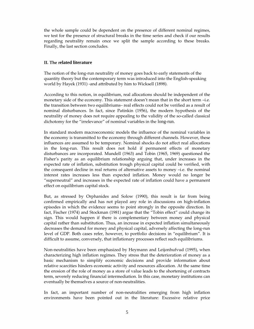
Argentina holds the dubious honor of having one of the highest inflation records internationally. The annual rate of inflation was 35.5% on average in the period considered in this study. However, as discussed in detail in the following sections, throughout this long period there have been very different nominal regimes. Until the first half of last century Argentina experienced very low inflation (the average annual rate was 1.7%), partially explained by the presence of several deflationary records. As a result inflation variability was significantly high in this period (a standard deviation of 8% and a coefficient of variation 4%). Since 1945 inflation became moderate and chronic (annual inflation was on average 25.9%) until the mid-seventies. In 1975, after a period of price controls and strong repressed inflationary pressures, the economy experienced an inflationary outburst. This episode, known as the Rodrigazo, decisively led the economy to a period of high inflation that lasted fifteen years and culminated in hyperinflationary episodes in 1989/1990. During this chaotic period, inflation registered annual records of three digits associated with the monetization of significant fiscal deficits and exhibited an extremely high variability (st. dev. of 800%). In 1991, the implementation of the currency board, “the Convertibility Plan”, and a broad economic reform allowed the economy to reach a stage of greater nominal stability, achieving one digit inflation for eight years. This scheme ended in an economic and financial crisis in 2001, leading the peso to a sharp depreciation along 2002. Contrary to expectations based on the previous inflationary history of Argentina, the sharp depreciation of the peso did not imply the acceleration in inflation in the aftermath of the crisis. However, during the 2000s, inflation rates have grown back to persistently moderate levels after 2007. As can be seen from Figure 1, prices followed very closely the dynamics of money. For the whole period under analysis, money, measured by M3 bimonetary, recorded an annual average increase of 39%.

Figure 1: Money and prices in logs. 1900-2012

-30

-20

-10

0

10

20

30

1900

1910

1920

1930

1940

1950

1960

1970

1980

1990

2000

2010

Log(M3 bim)Log(CPI)

(Log

sof

CP

I, M

3 b

im.)

-30

-20

-10

0

10

20

30

1900

1910

1920

1930

1940

1950

1960

1970

1980

1990

2000

2010

Log(M3 bim)Log(CPI)

-30

-20

-10

0

10

20

30

1900

1910

1920

1930

1940

1950

1960

1970

1980

1990

2000

2010

Log(M3 bim)Log(CPI)

-30

-20

-10

0

10

20

30

1900

1910

1920

1930

1940

1950

1960

1970

1980

1990

2000

2010

Log(M3 bim)Log(CPI)

(Log

sof

CP

I, M

3 b

im.)

This chaotic nominal evolution implied large transfers of wealth. In different inflationary episodes, holders of domestic financial assets have experienced very significant capital losses. Since real interest rates were mostly negative in times of high inflation (see Figure 2). Thus, not only holdings of currency suffered these losses but also holding in saving accounts and time deposits. Figure 3 shows money holdings

10

losses in terms of GDP of different monetary aggregates experienced by the public between 1901 and 2012.2,3

Figure 2: Real deposit interest rates (annual %) 1901-2012

-100%

-80%

-60%

-40%

-20%

0%

20%

40%

1901

1905

190919

13191

719

2119

2519

2919

3319

37194

119

4519

4919

5319

57196

119

65196

919

73197

719

81198

519

8919

9319

9720

0120

0520

09

(An

nua

l%)

-100%

-80%

-60%

-40%

-20%

0%

20%

40%

1901

1905

190919

13191

719

2119

2519

2919

3319

37194

119

4519

4919

5319

57196

119

65196

919

73197

719

81198

519

8919

9319

9720

0120

0520

09-100%

-80%

-60%

-40%

-20%

0%

20%

40%

1901

1905

190919

13191

719

2119

2519

2919

3319

37194

119

4519

4919

5319

57196

119

65196

919

73197

719

81198

519

8919

9319

9720

0120

0520

09-100%

-80%

-60%

-40%

-20%

0%

20%

40%

1901

1905

190919

13191

719

2119

2519

2919

3319

37194

119

4519

4919

5319

57196

119

65196

919

73197

719

81198

519

8919

9319

9720

0120

0520

09

(An

nua

l%)

2 Note that transfers of wealth have been from the holders of monetary assets to the issuers of such instruments: the government in the case of currency in circulation and banks in the case of deposits. That is, the public sector “shared” in many cases the inflation tax with financial institutions. However, sometimes the mechanism used by the government to capture some of that revenue has been raising reserve requirements of entities (although at some stages they have earned interests). See Brock (1989). 3 The inflation tax of the different aggregates was estimated according to the following

calculation: - For currency in circulation and current account deposits:

t

t

t

t

P

M

ππ+1

where:

tM is currency in circulation or deposits in period t .

tP is the consumer price index in t and tπ is the inflation rate in t .

t is measure in years (from 1941 on is measure in months, because data is available and

monthly frequency becomes more relevant for periods of high inflation). - For fixed time deposits and savings accounts, the corresponding nominal interest rate was taken into account:

t

tt

t

t i

P

M

ππ

+−

1 where:

ti is the relevant nominal interest rate.

11

Figure 3: Inflation tax (% of GDP) 1901-2012

-15%

-10%

-5%

0%

5%

10%

15%

20%

25%

30%

35%

1901

1906

1911

1916

1921

1926

1931

1936

1941

1946

1951

1956

1961

1966

1971

1976

1981

1986

1991

1996

2001

2006

2011

Inflation tax - M3

Inflation tax - M2

Inflation tax - M1

Inflation tax – Currency

(% o

fG

DP

)

-15%

-10%

-5%

0%

5%

10%

15%

20%

25%

30%

35%

1901

1906

1911

1916

1921

1926

1931

1936

1941

1946

1951

1956

1961

1966

1971

1976

1981

1986

1991

1996

2001

2006

2011

Inflation tax - M3

Inflation tax - M2

Inflation tax - M1

Inflation tax – Currency

-15%

-10%

-5%

0%

5%

10%

15%

20%

25%

30%

35%

1901

1906

1911

1916

1921

1926

1931

1936

1941

1946

1951

1956

1961

1966

1971

1976

1981

1986

1991

1996

2001

2006

2011

Inflation tax - M3

Inflation tax - M2

Inflation tax - M1

Inflation tax – Currency

(% o

fG

DP

)

Along with the mentioned nominal instability, monetary aggregates to GDP ratios showed a trend towards monetization until the mid 40s, a demonetization phase during the moderate and high inflation periods reaching a minimum level at the end of the 80s with the hyperinflation episodes, and a new monetization stage afterwards, in a context of strong volatility alongside this trends (see Figure 4).

Figure 4: Ratios of monetary aggregates to GDP

1900-2012

0%

5%

10%

15%

20%

25%

30%

35%

40%

45%

50%

1900

190419

0819

12191

619

2019

2419

2819

32193

619

4019

44194

819

5219

5619

6019

6419

6819

7219

7619

8019

8419

88199

219

9620

00200

420

0820

12

M1 bim. M3 bim.

(% o

fGD

P)

0%

5%

10%

15%

20%

25%

30%

35%

40%

45%

50%

1900

190419

0819

12191

619

2019

2419

2819

32193

619

4019

44194

819

5219

5619

6019

6419

6819

7219

7619

8019

8419

88199

219

9620

00200

420

0820

12

M1 bim. M3 bim.

(% o

fGD

P)

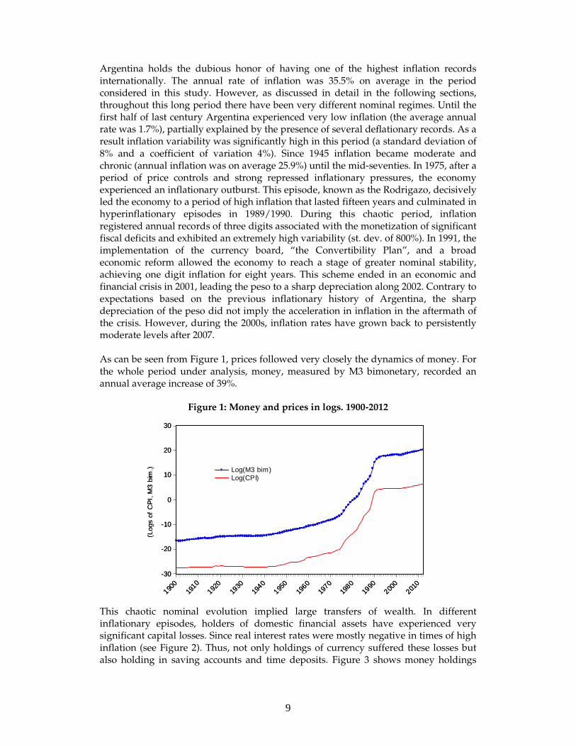
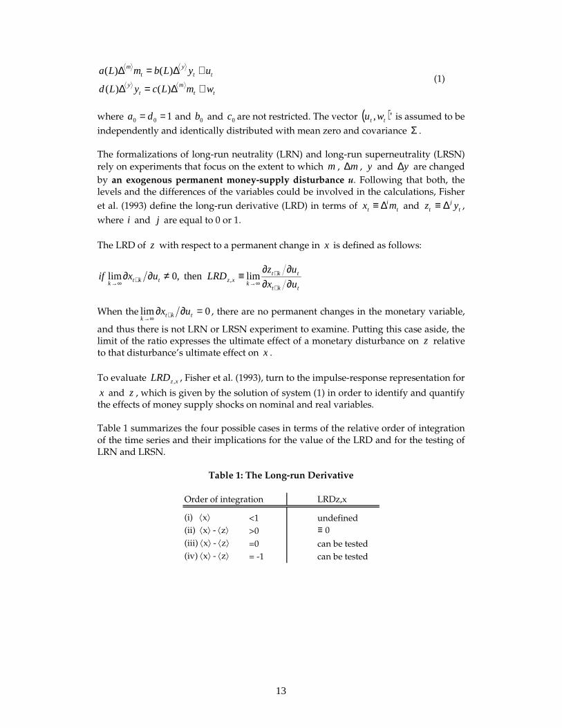
A first approach to study neutrality is to look at the relationship between money growth and inflation and money growth and GDP growth. Figure 5 shows that the linear correlation for the whole sample between annual money growth and inflation is quite strong (0.97); while is negative and near zero between annual changes of GDP and money growth (-0.16). In the next section we will draw on a methodology to analyze in a more rigorously and systematic way these correlations.

Figure 5: Changes in money, prices and GDP

12

(1900-2012)

-0.5

0.0

0.5

1.0

1.5

2.0

2.5

3.0

3.5

0 1 2 3

Dlog(M3 bim)

Dlo

g(C

PI)

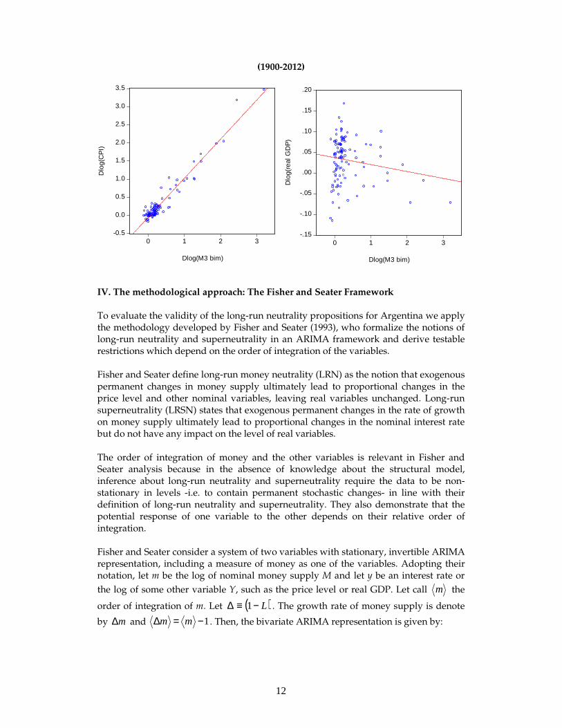
IV. The methodological approach: The Fisher and Seater Framework To evaluate the validity of the long-run neutrality propositions for Argentina we apply the methodology developed by Fisher and Seater (1993), who formalize the notions of long-run neutrality and superneutrality in an ARIMA framework and derive testable restrictions which depend on the order of integration of the variables. Fisher and Seater define long-run money neutrality (LRN) as the notion that exogenous permanent changes in money supply ultimately lead to proportional changes in the price level and other nominal variables, leaving real variables unchanged. Long-run superneutrality (LRSN) states that exogenous permanent changes in the rate of growth on money supply ultimately lead to proportional changes in the nominal interest rate but do not have any impact on the level of real variables. The order of integration of money and the other variables is relevant in Fisher and Seater analysis because in the absence of knowledge about the structural model, inference about long-run neutrality and superneutrality require the data to be non-stationary in levels -i.e. to contain permanent stochastic changes- in line with their definition of long-run neutrality and superneutrality. They also demonstrate that the potential response of one variable to the other depends on their relative order of integration. Fisher and Seater consider a system of two variables with stationary, invertible ARIMA representation, including a measure of money as one of the variables. Adopting their notation, let m be the log of nominal money supply M and let y be an interest rate or

the log of some other variable Y, such as the price level or real GDP. Let call m the

order of integration of m. Let ( )L−≡∆ 1 . The growth rate of money supply is denote

by m∆ and 1−=∆ mm . Then, the bivariate ARIMA representation is given by:

-.15

-.10

-.05

.00

.05

.10

.15

.20

0 1 2 3

Dlog(M3 bim)

Dlo

g(re

al G

DP

)

13

ttm

ty

tty

tm

wmLcyLd

uyLbmLa

+∆=∆

+∆=∆

)()(

)()( (1)

where 100 == da and 0b and 0c are not restricted. The vector ( )', tt wu is assumed to be

independently and identically distributed with mean zero and covariance Σ . The formalizations of long-run neutrality (LRN) and long-run superneutrality (LRSN)

rely on experiments that focus on the extent to which m , m∆ , y and y∆ are changed

by an exogenous permanent money-supply disturbance u. Following that both, the levels and the differences of the variables could be involved in the calculations, Fisher

et al. (1993) define the long-run derivative (LRD) in terms of ti

t mx ∆≡ and tj

t yz ∆≡ ,

where i and j are equal to 0 or 1.

The LRD of z with respect to a permanent change in x is defined as follows:

tkt

tkt

kxztkt

k ux

uzLRDuxif

∂∂∂∂

≡≠∂∂+

+

∞→+∞→limthen ,0lim ,

When the 0lim =∂∂ +∞→ tktk

ux , there are no permanent changes in the monetary variable,

and thus there is not LRN or LRSN experiment to examine. Putting this case aside, the limit of the ratio expresses the ultimate effect of a monetary disturbance on z relative to that disturbance’s ultimate effect on x .

To evaluate xzLRD , , Fisher et al. (1993), turn to the impulse-response representation for

x and z , which is given by the solution of system (1) in order to identify and quantify the effects of money supply shocks on nominal and real variables. Table 1 summarizes the four possible cases in terms of the relative order of integration of the time series and their implications for the value of the LRD and for the testing of LRN and LRSN.

Table 1: The Long-run Derivative

Order of integration LRDz,x

(i) ⟨x⟩ <1 undefined

(ii) ⟨x⟩ - ⟨z⟩ >0 ≡ 0(iii) ⟨x⟩ - ⟨z⟩ =0 can be tested

(iv) ⟨x⟩ - ⟨z⟩ = -1 can be tested

14

a. Long-run neutrality

LRN definition: Money is long-run neutral if λ=myLRD , where 1=λ when y is a

nominal variable and 0=λ when y is a real variable. As can been seen from Table 1, the four possible cases for the order of integration should be analyzed in order to get the LRN.

Case (i): when m is less than one, myLRD , is not defined, simply because there are no

permanent shocks in the level of money stock, so LRN is meaningless.

Case (ii): when 11≥+≥ ym , 0, ≡myLRD . In this case there are permanent shocks to

the level of money stock, but there can’t be permanent shocks to y. Therefore the LRN holds when y is a real variable or the nominal interest rate. However, if y is a nominal variable, LRN is violated.

Case (iii): when 1≥= ym . myLRD , can be tested in order to find out if the

permanent shocks to the level of money stocks are correlated with permanent shocks to

the variable y. If 1== ym , a test of LRN is possible because there are permanent

changes in m and y. On the other hand, if 2== ym , there are permanent change in

the growth rates of both m and y. In this case we have that mymy LRDLRD ,, =∆∆ . This

direct translation means that growth-rate-to-growth-rate propositions are not LRSN propositions, even though they involve changes in growth rate of money; rather they are equivalent to level-to-level LRN.

Case (iv): when 11≥−≥ ym , which is equivalent to 1≥∆= ym . myLRD , can be

tested although this case is uncommon. A necessary condition for long run neutrality is that the permanent shocks to money do not change the growth rate of y. Concerning LRSN, we will analyze how the effects of permanent shocks in the growth rate of money change the level of other variables. b. Long-run superneutrality

LSRN definition: Money is long-run superneutral if µ=∆myLRD , where 1=µ when y

is the nominal rate of interest and 0=µ when y is a real variable.

The definition of LRSN only applies to those variables y for which LRN implies

LRDy,m=0. The implications µ=∆myLRD , are also analyzed for the four cases of the

Table 1.

Case (i): when m∆ is less than one (i.e. m is less than two), myLRD ∆, is not defined.

LRSN is meaningless.

15

Case (ii): when 11≥+≥∆ ym (i.e. 22 ≥+≥ ym ), 0, ≡∆myLRD . When

2=m and 0=y , permanent changes in m∆ cannot be associated with nonexistent

changes in y.

Case (iii): when 1≥=∆ ym (i.e. 21≥+≥ ym ), myLRD ∆, can be tested, even

though LRN cannot be rejected because 0, ≡myLRD .

Case (iv): when 11≥−=∆ ym (i.e. 2≥= ym ), myLRD ∆, can be tested. Note that

in this case we can check the LRN of m with respect to y which can be expressed as

0, =∆∆ myLRD , stating that the growth rate of y remains unchanged in the long run.

Thus, LRSN can be evaluated only if LRN holds; or equivalently if LRN does not hold, LRSN cannot hold. However, if LRN holds, this does not imply that LRSN should hold. Table 2 below summarizes the results for LRN and LRSN.

Table 2: Long-Run Neutrality and Superneutrality Restrictions

⟨y⟩ ⟨m⟩=0 ⟨m⟩=1 ⟨m⟩=2 ⟨m⟩=0 ⟨m⟩=1 ⟨m⟩=2

0 undefined ≡ 0 ≡ 0 undefined undefined ≡ 0

1 undefined can be tested ≡ 0 undefined undefined can be tested

2 undefined can be tested can be tested undefined undefined can be tested

LRDy,∆mLRDy,m

LRN → LRDy,m = λ LRN → LRDy,∆m = µ

How to evaluate the LRD empirically

In order to test LRN or LRSN, the LRD should be evaluated. Fisher and Seater (1993) propose to use the Barlett estimator of the frequency-zero regression coefficient, in the

regression of yy∆ on mm∆ . This estimator is given by kk

β∞→

lim where kβ is the slope

coefficient from the regression:

( ) ( ) ktkttkkktt emmyy +−+=− −−−− 11 βα (2)

when 1== my .

According to (2), kb is the slope between the money growth rates and y growth rates.

The Barlett estimator is the limit of this slope as the span over which those growth rates are computed goes to infinity.

On the other hand, when 1=y and 2=m , the regression is:

( ) ( ) ktkttkkktt emmyy +∆−∆+=− −−−− 11 βα (3)

and kβ has a similar interpretation.

16

The estimates of kβ were obtained for k=1,…,30 and a 95% confidence intervals

corrected by Newey and West (1987) technique, which were constructed from a t distribution using the number of observation divided by k as degrees of freedom. In the next section we analyze the order of integration for the different monetary aggregates, prices and real GDP.4 Testing unit roots The order of integration of the time series of interest is a key feature that should be analyzed carefully to carry out the empirical analysis. Many macroeconomic series show a high degree of persistence, and sometimes it becomes quite difficult to distinguish between a high degree of persistence and a permanent shock. Unit roots diagnostics tests have been designated to classify macroeconomic variables into those that have been subject to permanent shocks and those that have not. Nevertheless, these kinds of tests are far from perfect and face empirical limitations. As pointed out by Maddala and Kim (2004) some of these tests have problems of low power -e.g. the augmented Dickey- Fuller (ADF) test- or size distortions -e.g. the Phillips-Perron (PP) test-. Taking into account the Monte Carlo evidence showed in the literature (Schwert, 1989; De Jong, 1992; Agiakoglou and Newbold, 1992), and following Maddala et al. (2004) advice, we have decided not to use the popular ADF neither PP unit root tests.5 Given that one of the central problems with unit root tests based in autorregresive processes are MA errors, the original PP test was designed to pay attention to MA errors. Even so, it suffers from severe size distortions when the MA root parameter is large (Schwert, 1989). For this reason, useful modifications of these tests are evaluated below. Ng and Perron (2001) proposed modifications of the PP test to correct the size distortions caused by

MA errors. Two modified versions of PP test, αMZ and tMZ statistics, are presented

based upon GLS detrended data.6 Furthermore the test developed by Elliot, Rothenberg and Stock (1996), henceforth ERS, is tested as well. The ERS test is a modification of the ADF test, and it has the advantage of being the second best when uniformly most powerful test does not exist.7 This test is also based on the quasi-differencing regression like the modified versions of PP test. Thereby and using these challenging developments in unit root tests we will evaluate the stochastic behavior of the data under study namely, monetary aggregates, prices and real GDP.

4 Our sample, as Fisher et. al (1993) sample, are annual data that includes more than one

hundred observations. Like them, we consider till k=30 as the empirical limit of kβ . 5 In Maddala and Kim (2004), chapter 4, the authors said “…hence, ADF and PP test, still often used, should be discarded in favor of these tests (referring to the PP and ADF modification’s tests)”. 6 Elliot, Rothenterberg and Stock (1996) define a quasi-difference of yt in order to detendred the data, so that the explanatory variables (constant or/and lineal trend) are taken out of the data prior to running the unit root test regression. 7 Uniformly most powerful test does not exist for the unit root hypothesis. A consequence of this fact is the large number of unit root tests on the literature. See Stock, 1994, and Maddala and Kim, 2004.

17

In Table 3 the results of the Ng-Perron tests for the annual consumer price index (CPI) are shown for the sample 1900-2012. As can seen from the table, in the case of the log level of the CPI, both statistic tests fall inside de acceptance region (they do not reject the null hypothesis of a unit root), regardless the test specification has a constant (the

reader should compare the αMZ =1.760 and tMZ =1.641 against Ng-Perron critical

value at 5%, -8.10 and -1.98 respectively) or has a constant and a linear trend (in this

case one should compare the αMZ =-1.471 and tMZ =-0.753 against Ng-Perron

asymptotic critical value at %5, -17.30 and -2.91 respectively). When the difference in CPI logs is tested, the results depend on the test specification: (i) a constant or (ii) a constant plus a linear trend. In the (i) case, both modified versions of PP test give the same conclusions at any level of significance -i.e. they reject the null hypothesis of unit root-. On the other hand, in the (ii) case, the presence of a unit root at 5% significance level for both tests is rejected, but when the significance level is 1% the null hypothesis is not rejected. In fact, the presence of a linear trend in the inflation rate is not a realistic assumption, moreover when the span is a century. This result could be biased by the presence of structural breaks possibly related to different macroeconomic regimes, as will be shown bellow. Looking at the second difference of the log of CPI, both statistics reject the null hypothesis of a unit root at any significance level.8

Table 3: Ng-Perron unit root tests for Consumer Price Index

Unit root tests

H0: the series has a unit root

Sample: 1900-2012

Bandwidth: Andrews automatic using Bartlett kernel

MZa MZt MZa MZt

Log(CPI) 1.760 1.641 -1.471 -0.753

∆Log(CPI) -16.714 -2.891 -19.706 -3.126

∆∆Log(CPI) -55.710 -5.276

1% -13.80 -2.58 -23.80 -3.42

5% -8.10 -1.98 -17.30 -2.91

10% -5.70 -1.62 -14.20 -2.62

HAC corrected variance (Bartlett kernel)

Exogenous: constantExogenous: constant and

linear trend

Asymptotic critical

values, Ng-Perron

(2001, Table 1)

Ng-Perron test

Table 4 shows the unit root test for the CPI according to Elliot, Rothenberg and Stock (1996). The statistical conclusions from ERS tests are exactly the same as Ng-Perron tests. Thus, whether the inflation rate could have or not a linear trend, the CPI would be considered I(2) or I(1) respectively.

8 We do not show the results for the second difference of log of CPI with the specification with constant and linear trend because it does not make any economic sense.

18

Table 4: ERS unit root tests for Consumer Price Index

Unit root testsH0: the series has a unit root

Sample: 1900-2012

Bandwidth: Andrews automatic using Bartlett kernel

Log(CPI)

∆Log(CPI)

∆∆Log(CPI)

1%

5%

10%

HAC corrected variance (Bartlett kernel)

0.447

Asymptotic critical

values, Elliott-

Rothenberg-Stock

(1996, Table 1)

1.95 4.23

3.12 5.64

4.19 6.80

79.750 55.499

1.470 4.641

Elliott-Rothenberg-Stock

Test

Exogenous: constantExogenous: constant and

linear trend

ERS test ERS test

Tables 5 and 6 present the same type of unit root analysis for the remaining nominal variables. As can be seen from Table 3, currency, M1, M2 and M3 do not show a clear-cut if they should be treated as I(1) or I(2) variables. Working at 5% level of significance, the null hypothesis of the presence of a unit root in the logs differences

should be rejected, for all variables for both statistics ( αMZ and tMZ ). As a

consequence, all variables should be considered I(1), regardless the exogenous variables added to the specification test. In contrast, if the 1% level of significance is considered, the presence of a unit root in the logs differences of currency, M1, M2 and M3 would not be rejected and they should be considered I(2). On the other hand, the monetary base is clearly I(1), for both modified versions of PP test, despite the exogenous variables included in the test specification.

19

Table 5: Ng-Perron unit root tests for monetary aggregates

Unit root tests

H0: the series has a unit root

Sample: 1900-2012

Bandwidth: Andrews automatic using Bartlett kernel

MZa MZt MZa MZt

Log(Currency) 1.989 2.065 -1.299 -0.681

∆Log(Currency) -9.190 -2.124 -17.732 -2.953

∆∆Log(Currency) -42.408 -4.597

Log(Mon_base) 1.982 2.192 -1.286 -0.687

∆Log(Mon_base) -22.350 -3.342 -27.262 -3.680

Log(M1) 2.014 2.164 -1.283 -0.677

∆Log(M1) -11.816 -2.420 -19.154 -3.074

∆∆Log(M1) -52.253 -5.108

Log(M2) 2.005 2.143 -1.364 -0.706

∆Log(M2) -11.863 -2.428 -18.467 -3.015

∆∆Log(M2) -54.787 -5.231

Log(M3) 1.935 1.999 -1.462 -0.743

∆Log(M3) -10.361 -2.270 -15.906 -2.792

∆∆Log(M3) -55.505 -57.730

1% -13.80 -2.58 -23.80 -3.42

5% -8.10 -1.98 -17.30 -2.91

10% -5.70 -1.62 -14.20 -2.62

HAC corrected variance (Bartlett kernel)

Exogenous: constant and

linear trend

Asymptotic critical

values, Ng-Perron

(2001, Table 1)

Ng-Perron testExogenous: constant

The ERS unit root tests give the same conclusions as the Ng-Perron tests for all variables but currency. As the Table 6 shows, in the case of currency, there is even more evidence that this variable could be treated as I(2). The ERS test with a constant is equal to 3.279 over the 5% level of significance (3.12); hence the unit root at 5% level should not be rejected.

20

Table 6: ERS unit root tests for monetary aggregates

Unit root testsH0: the series has a unit root

Sample: 1900-2012

Bandwidth: Andrews automatic using Bartlett kernel

Log(Currency)

∆Log(Currency)

∆∆Log(Currency)

Log(Mon_base)

∆Log(Mon_base)

Log(M1)

∆Log(M1)

∆∆Log(M1)

Log(M2)

∆Log(M2)

∆∆Log(M2)

Log(M3)

∆Log(M3)

∆∆Log(M3)

1%

5%

10%

HAC corrected variance (Bartlett kernel)

60.840

1.119 3.360

59.215

3.279 5.310

0.684

Elliott-Rothenberg-Stock

Test

Exogenous: constantExogenous: constant and

linear trend

ERS test ERS test

5.817

109.530

2.404

0.498

108.551

2.341

0.467

100.648

2.641

57.154

5.022

54.886

4.23

5.64

6.80

59.807

4.836

Asymptotic critical

values, Elliott-

Rothenberg-Stock

(1996, Table 1)

1.95

3.12

4.19

0.460

101.862

115.263

Looking at real variables, both GDP and real balances are undoubtedly I(1) variables regardless of the exogenous variables specified in the unit root test (see Table 7).

Table 7: Ng-Perron and ERS unit root tests for real variables

Unit root tests

H0: the series has a unit root

Sample: 1900-2012

Bandwidth: Andrews automatic using Bartlett kernel

MZa MZt MZa MZt

Log(Real GDP) 1.550 4.099 -4.969 -1.515 Log(Real GDP)

∆Log(Real GDP) -40.260 -4.453 -51.181 -5.058 ∆Log(Real GDP)

Log(Real balances - M3) 0.888 0.688 -8.913 -2.111 Log(Real balances - M3)

∆Log(Real balances - M3) -25.667 -3.565 -41.550 -4.554 ∆Log(Real balances - M3)

1% -13.80 -2.58 -23.80 -3.42 1%

5% -8.10 -1.98 -17.30 -2.91 5%

10% -5.70 -1.62 -14.20 -2.62 10%

HAC corrected variance (Bartlett kernel)

Asymptotic critical

values, Elliott-

Rothenberg-Stock

(1996, Table 1)

1.95 4.23

3.12 5.64

4.19 6.80

58.328 10.872

1.294 2.447

663.480 21.714

0.809 1.797

Elliott-Rothenberg-Stock

Test

Exogenous:

constant

Exogenous: constant

and linear trend

ERS test ERS test

Exogenous: constant and

linear trend

Asymptotic critical

values, Ng-Perron

(2001, Table 1)

Ng-Perron testExogenous: constant

21

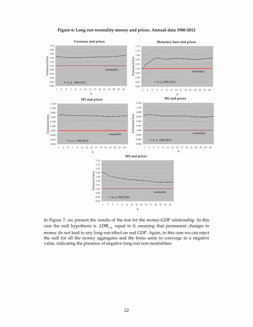
V. Empirical results Following Fisher and Seater (1993), we use the Barlett estimator to calculate de long-run derivate LRD according to equations (2) and (3) depending on the order of integration of the respective time series.9 We consider the five money aggregates described above: Currency in circulation, the monetary base, M1, M2 and M3 and test the validity of long-run neutrality hypothesis with respect to both prices and real GDP.10 Figure 6 shows the results of the long-run neutrality test of the five money aggregates with respect to prices, in particular, the evolution of the betas considering 1 to 30 lags

and its appropriate confidence intervals. The null hypothesis is mpLRD , equal to 1, i.e.

permanent changes in the money supply should lead in the long run to changes of equal magnitude in prices. In all cases the null is rejected and the estimated betas seem to converge to a value that exceeds 1, indicating that the relationship between different measures of money and prices is more than proportional.

9 It is important to remember that this methodology assumes explicitly that innovations in the monetary process are exogenous to the other variables in the exercise, something that we are not questioning here. 10 These variables are defined in the Appendix.

22

Figure 6: Long run neutrality money and prices. Annual data 1900-2012

Monetary base and prices

0.90

0.93

0.95

0.98

1.00

1.03

1.05

1.08

1.10

1.13

1 3 5 7 9 11 13 15 17 19 21 23 25 27 29

k

Est

imat

ed

be

ta

b_k 1900-2012

neutrality

M1 and prices

0.940

0.960

0.980

1.000

1.020

1.040

1.060

1.080

1.100

1.120

1 3 5 7 9 11 13 15 17 19 21 23 25 27 29

k

Est

imat

ed b

eta

b_k 1900-2012

neutrality

M2 and prices

0.940

0.960

0.980

1.000

1.020

1.040

1.060

1.080

1.100

1.120

1 3 5 7 9 11 13 15 17 19 21 23 25 27 29

k

Est

imat

ed b

eta

b_k 1900-2012

neutrality

M3 and prices

0.94

0.96

0.98

1.00

1.02

1.04

1.06

1.08

1.10

1.12

1.14

1 3 5 7 9 11 13 15 17 19 21 23 25 27 29

k

Est

ima

ted

bet

a

b_k 1900-2012

neutrality

Currency and prices

0.90

0.92

0.94

0.96

0.98

1.00

1.02

1.04

1.06

1.08

1.10

1 3 5 7 9 11 13 15 17 19 21 23 25 27 29

k

Est

ima

ted

bet

a

b_k 1900-2012

neutrality

In Figure 7, we present the results of the test for the money-GDP relationship. In this

case the null hypothesis is myLDR , equal to 0, meaning that permanent changes in

money do not lead to any long-run effect on real GDP. Again, in this case we can reject the null for all the money aggregates and the betas seem to converge to a negative value, indicating the presence of negative long-run non-neutralities.

23

Figure 7: Long run neutrality money and real GDP. Annual data 1900-2012

Monetary base and real GDP

-0.035

-0.030

-0.025

-0.020

-0.015

-0.010

-0.005

0.000

1 3 5 7 9 11 13 15 17 19 21 23 25 27 29

k

Est

imat

ed b

eta

b_k 1900-2012

neutrality

M1 and real GDP

-0.035

-0.030

-0.025

-0.020

-0.015

-0.010

-0.005

0.000

1 3 5 7 9 11 13 15 17 19 21 23 25 27 29

k

Est

imat

ed b

eta

b_k 1900-2012

neutrality

bo

M2 and real GDP

-0.035

-0.030

-0.025

-0.020

-0.015

-0.010

-0.005

0.000

1 3 5 7 9 11 13 15 17 19 21 23 25 27 29

k

Est

imat

ed b

eta

b_k 1900-2012

neutrality

M3 and real GDP

-0.035

-0.030

-0.025

-0.020

-0.015

-0.010

-0.005

0.000

1 3 5 7 9 11 13 15 17 19 21 23 25 27 29

k

Est

imat

ed b

eta

b_k 1900-2012

neutrality

Currency and real GDP

-0.035

-0.030

-0.025

-0.020

-0.015

-0.010

-0.005

0.000

1 3 5 7 9 11 13 15 17 19 21 23 25 27 29

k

Est

imat

ed b

eta

b_k 1900-2012

neutrality

These results are not completely novel. In fact, Bae et al. (2000) using the same methodology to study long-run money neutrality in Argentina and Brazil during the period 1884-1996 have a similar result: Money is neutral with respect to output in both countries, but not superneutral.11 They refer to this finding as an opposite “Tobin effect”. They check if the rejection of long-run superneutrality is related to the presence of anomalous events. In order to control for these events, they introduce intercept dummies for banking crisis episodes.12 The introduction of these dummies does not change their general results.

11 We do not test superneutrality for the whole period because we find that money is not long-run neutral with respect to both output and prices and, as mentioned before in Section IV, long-run neutrality is a necessary condition for long-run superneutrality. 12 In doing that, they follow Boscher and Ostrok (1994) and Haug and Lucas (1997).

24

We depart form their approach since our presumption is that the non neutralities found are related to the presence of structural breaks in the sample. Thus, we investigate the presence of structural breaks in the time series and their coincidence.13 In fact, pronounced coincident breaks in the time series of money and prices over the period 1900-2012 can be detected by simple visual inspection (see Figure 1). Additionally, the finding of a linear trend in inflation, difficult to explain from an intuitive point of view, suggests the presence of regimes changes. Structural breaks in money-prices relationship were studied by Basco et al. (2009) for the period 1977-2006. Also, D’Amato and Garegnani (2013), when studying inflation dynamics in Argentina over the period 1960-2006, identify structural breaks in this time series using the Bai-Perron test. In the following section we test for the presence of multiple breaks in money aggregates, prices and velocity to identify relevant sub-periods in the evolution of nominal variables.14 Our guess is that these breaks would probably be related to relevant changes in nominal regimes that can be identified with a narrative description of the evolution of monetary frameworks in Argentina. Identifying structural breaks in time series To test for the presence of multiple breaks we appeal to the battery of tests developed by Bai and Perron (1998, 2003), which are quite general and flexible, something particularly attractive for the time series of Argentina. The Bai-Perron (1998, 2003) methodology allows estimating multiple partial breaks for a subset of parameters in linear models. Thus, the method can be applied to pure or partial structural change models. Bai et al. (1998, 2003) also developed a procedure to construct confidence intervals for break dates, allowing for different distribution for the data and errors and different serial correlation in the errors as well. They provide three type of tests: (i) a test of no break vs. a fixed number of breaks, (ii) two tests of no break against an unknown number of breaks, the Double Maximum Tests and (iii) and a sequential test of l versus l+1 breaks, to select the number of breaks which has advantage relative to information criterion as BIC and LWZ, since it takes into account potential heterogeneity across segments. Given the changing dynamics of the time series of nominal variables in Argentina, we choose the most flexible estimation procedure. Thus, we test breaks in the mean values of the time series of money aggregates, prices, velocity. In all cases the regression model adjusted was an autoregressive process with one lag and a HAC covariance to

13 As a cross check exercise, we introduced intercept dummy variables to control for crisis and anomalous periods. Similar to the findings of Bae and Ratti (2000) these controls are statistically significant but do not change the non neutrality results. The results of this exercise are disposable upon request 14 In spite of not being a nominal variable, we study the behavior of money velocity too. The reason is that this variable resumes the evolution of real GDP and money real balances and can give us a sense of the response of the public in terms of money demand to the signals coming from nominal (and real) instability.

25

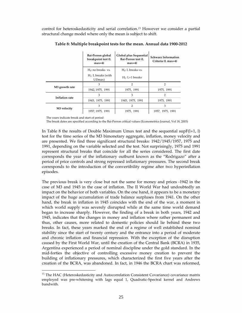
control for heteroskedasticity and serial correlation.15 However we consider a partial structural change model where only the mean is subject to shift.

Table 8: Multiple breakpoint tests for the mean. Annual data 1900-2012

Bai-Perron global

breakpoint test (L

max=4)

Global plus Sequential

Bai-Perron test (L

max=4)

Schwarz Information

Criteria (L max=4)

H0: no breaks vs. H0: L breaks vs.

H1: L breaks (with

UDmax)H1: L+1 breaks

3 2 2

1942, 1975, 1991 1975, 1991 1975, 1991

3 3 2

1945, 1975, 1991 1945, 1975, 1991 1975, 1991

3 2 3

1957, 1975, 1991 1975, 1991 1957, 1975, 1991

The years indicate break and start of period

The break dates are specified according to the Bai-Perron critical values (Econometrics Journal, Vol 18, 2003)

M3 growth rate

Inflation rate

M3 velocity

In Table 8 the results of Double Maximum Umax test and the sequential supF(l+1, l) test for the time series of the M3 bimonetary aggregate, inflation, money velocity and are presented. We find three significant structural breaks: 1942/1945/1957, 1975 and 1991, depending on the variable selected and the test. Not surprisingly, 1975 and 1991 represent structural breaks that coincide for all the series considered. The first date corresponds the year of the inflationary outburst known as the “Rodrigazo” after a period of price controls and strong repressed inflationary pressures. The second break corresponds to the introduction of the convertibility regime after two hyperinflation episodes. The previous break is very close but not the same for money and prices -1942 in the case of M3 and 1945 in the case of inflation. The II World War had undoubtedly an impact on the behavior of both variables. On the one hand, it appears to be a monetary impact of the huge accumulation of trade balance surpluses from 1941. On the other hand, the break in inflation in 1945 coincides with the end of the war, a moment in which world supply was severely disrupted while at the same time world demand began to increase sharply. However, the finding of a break in both years, 1942 and 1945, indicates that the changes in money and inflation where rather permanent and thus, other causes, more related to domestic policies should lie behind these two breaks. In fact, these years marked the end of a regime of well established nominal stability since the start of twenty century and the entrance into a period of moderate and chronic inflation and financial repression. With the exception of the disruption caused by the First World War, until the creation of the Central Bank (BCRA) in 1935, Argentina experienced a period of nominal discipline under the gold standard. In the mid-forties the objective of controlling excessive money creation to prevent the building of inflationary pressures, which characterized the first five years after the creation of the BCRA, was abandoned. In fact, in 1946 the BCRA chart was reformed,

15 The HAC (Heteroskedasticity and Autocorrelation Consistent Covariance) covariance matrix employed was pre-whitening with lags equal 1, Quadratic-Spectral kernel and Andrews bandwith.

26

instituting a radically different monetary regime: deposits were nationalized and commercial banks began to act as financial agents of the BCRA that was assigned the task of manipulating interest rates and directing credit to specific sectors of the economy, according to the objectives of the central government. In the case of money velocity there are three structural breaks: 1975 and 1991 –coincident with the other variables considered- and 1957. As mentioned above, the inflationary outburst of 1975 marked the beginning of a high inflation regime; and the adoption of Convertibility in 1991 led to a drastic disinflation. Both episodes had a dramatic impact on real money demand. As stressed by McCallum (1989) and others, rapid changes in trend inflation as those of 1975 and 1991 have a quite permanent impact on the desire of agents to maintain real money holdings, in the spirit of the Cagan (1956) model developed to describe hyperinflation episodes. The fact that money velocity does not break along with money and prices in the 40s can also be interpreted in the same spirit, since it was not until the end of the fifties that Argentina began to register truly high inflation records. In most part of this decade price controls and financial repression probably maintained real money holdings artificially high, but after 1955 a liberalization process began and key relative prices where allowed to adjust.16 Looking inside the periods Having identified the structural breaks in the time series of money, prices and money velocity, we now turn to evaluate if the non neutralities that we find for the complete sample are due to non neutralities in any of the sub-periods in which the breaks split the sample rather than a feature of the complete sample. Ideally, to be consistent with the identified structural breaks, the sample should be divided in four periods: 1900-1944, 1945-1974, 1975-1991 and 1992-2012,. But, using annual data, we lack of the degrees of freedom required to implement Fisher and Seater’s neutrality test. Thus, we first consider two periods: before and after 1975. We study the first one using annual data, since there are not reliable time series at a higher frequency for this period. This implies not being able to analyze the sub periods generated by the structural break around 1942 and 1945. The second period -1975-2012- can be splitted into the two remaining sub periods -1975-1991 and 1992-2012- and analyzed using quarterly data. We are aware that in this case we are relaying on observations at a higher frequency than desired to analyze long run phenomena. In fact, evaluating the limit of LRD for a k=30 is not the same when dealing with years than with quarters. However, we consider that a 30 quarters horizon is reasonable to evaluate long run responses. In Figure 8 and 9 we present the results of the test for the first sub period: 1900-1974. It can be seen from Figure 8, that shows the results for the money and price relationship, that the evidence is mixed: Permanent changes in money supply lead in the long-run to

16 After a big devaluation of the currency and tariffs increases as part of an IMF agreement, in 1959 Argentina experienced for the first time in its economic history a three digit inflation record (114% annually).

27

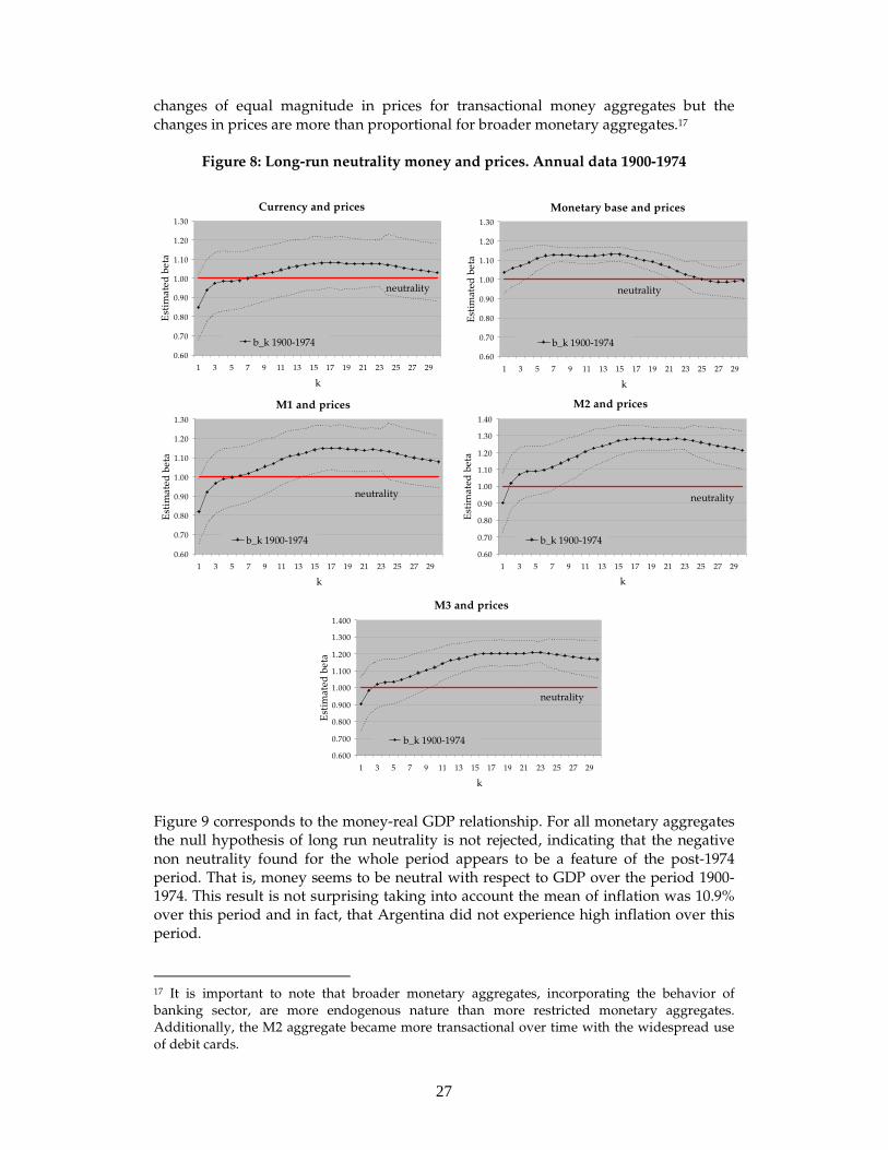
changes of equal magnitude in prices for transactional money aggregates but the changes in prices are more than proportional for broader monetary aggregates.17

Figure 8: Long-run neutrality money and prices. Annual data 1900-1974

Monetary base and prices

0.60

0.70

0.80

0.90

1.00

1.10

1.20

1.30

1 3 5 7 9 11 13 15 17 19 21 23 25 27 29

k

Est

imat

ed b

eta

b_k 1900-1974

neutrality

M1 and prices

0.60

0.70

0.80

0.90

1.00

1.10

1.20

1.30

1 3 5 7 9 11 13 15 17 19 21 23 25 27 29

k

Est

imat

ed b

eta

b_k 1900-1974

neutrality

M2 and prices

0.60

0.70

0.80

0.90

1.00

1.10

1.20

1.30

1.40

1 3 5 7 9 11 13 15 17 19 21 23 25 27 29

k

Est

imat

ed b

eta

b_k 1900-1974

neutrality

M3 and prices

0.600

0.700

0.800

0.900

1.000

1.100

1.200

1.300

1.400

1 3 5 7 9 11 13 15 17 19 21 23 25 27 29

k

Est

imat

ed b

eta

b_k 1900-1974

neutrality

Currency and prices

0.60

0.70

0.80

0.90

1.00

1.10

1.20

1.30

1 3 5 7 9 11 13 15 17 19 21 23 25 27 29

k

Est

imat

ed b

eta

b_k 1900-1974

neutrality

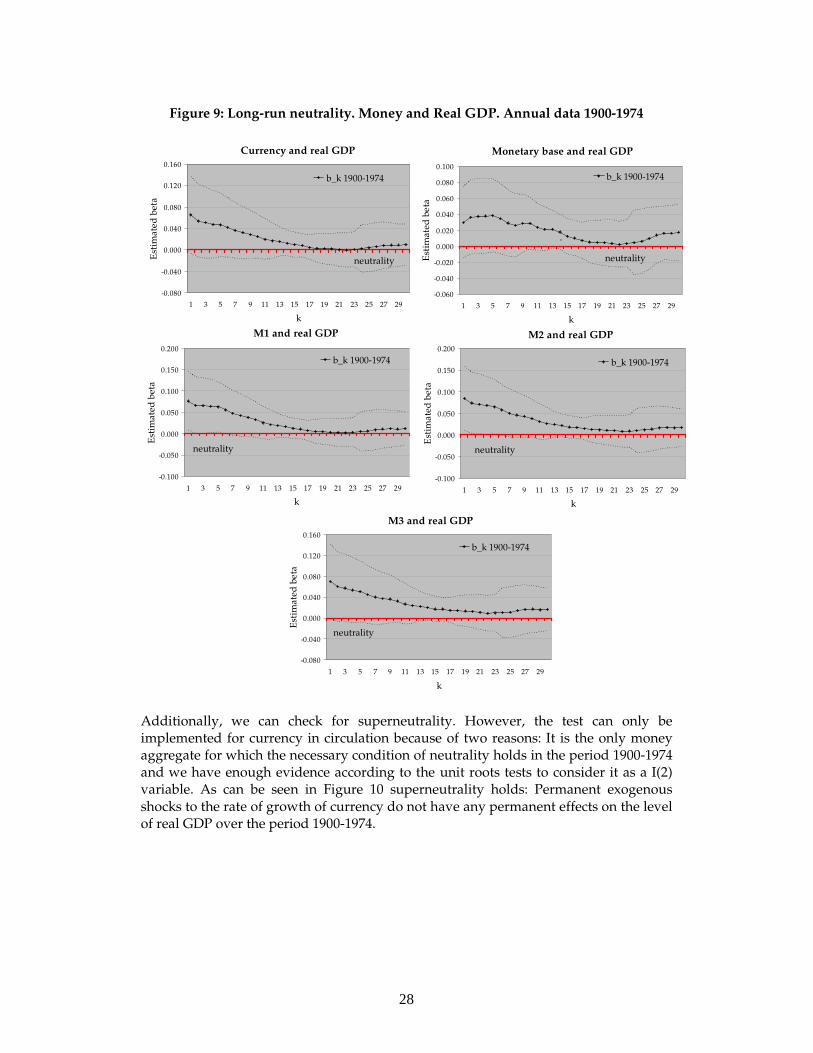
Figure 9 corresponds to the money-real GDP relationship. For all monetary aggregates the null hypothesis of long run neutrality is not rejected, indicating that the negative non neutrality found for the whole period appears to be a feature of the post-1974 period. That is, money seems to be neutral with respect to GDP over the period 1900-1974. This result is not surprising taking into account the mean of inflation was 10.9% over this period and in fact, that Argentina did not experience high inflation over this period.

17 It is important to note that broader monetary aggregates, incorporating the behavior of banking sector, are more endogenous nature than more restricted monetary aggregates. Additionally, the M2 aggregate became more transactional over time with the widespread use of debit cards.

28

Figure 9: Long-run neutrality. Money and Real GDP. Annual data 1900-1974

Monetary base and real GDP

-0.060

-0.040

-0.020

0.000

0.020

0.040

0.060

0.080

0.100

1 3 5 7 9 11 13 15 17 19 21 23 25 27 29

k

Est

imat

ed b

eta

b_k 1900-1974

a

neutrality

M1 and real GDP

-0.100

-0.050

0.000

0.050

0.100

0.150

0.200

1 3 5 7 9 11 13 15 17 19 21 23 25 27 29

k

Est

imat

ed b

eta

b_k 1900-1974

neutrality

M2 and real GDP

-0.100

-0.050

0.000

0.050

0.100

0.150

0.200

1 3 5 7 9 11 13 15 17 19 21 23 25 27 29

k

Est

ima

ted

bet

a

b_k 1900-1974

neutrality

M3 and real GDP

-0.080

-0.040

0.000

0.040

0.080

0.120

0.160

1 3 5 7 9 11 13 15 17 19 21 23 25 27 29

k

Est

imat

ed b

eta

b_k 1900-1974

neutrality

Currency and real GDP

-0.080

-0.040

0.000

0.040

0.080

0.120

0.160

1 3 5 7 9 11 13 15 17 19 21 23 25 27 29

k

Est

imat

ed

bet

a

b_k 1900-1974

neutrality

Additionally, we can check for superneutrality. However, the test can only be implemented for currency in circulation because of two reasons: It is the only money aggregate for which the necessary condition of neutrality holds in the period 1900-1974 and we have enough evidence according to the unit roots tests to consider it as a I(2) variable. As can be seen in Figure 10 superneutrality holds: Permanent exogenous shocks to the rate of growth of currency do not have any permanent effects on the level of real GDP over the period 1900-1974.

29

Figure 10: Long-run superneutrality. Currency and real GDP. Annual data 1900-1974

Solid line represents the estimated beta_k coefficients.

Dashed lines are the bound of the 95% confidence interval of the estimated coefficients

-0.8

-0.6

-0.4

-0.2

0.0

0.2

0.4

0.6

0.8

1.0

1 2 3 4 5 6 7 8 9 10 11 12 13 14 15 16 17 18 19 20 21 22 23 24 25 26 27 28 29 30

k

Est

imat

ed b

eta

beta_k 1900-1974

For the rest of the sample, 1975-2012 we can analyze the two indentified sub-periods: Before and after the two hyperinflation episodes. For the first sub-period (1975q1-1990q1) we perform two exercises: (i) including the two hyperinflation episodes, which are in fact very anomalous and transitory disruptions (1975q1-1990q1) and (ii) discarding them (1975q1-1988q4). For the second sub-period (1990q2-2012q4), we do a similar exercise: (iii) consider the period 1990q2 -2012q4, which includes the sharp decline of inflation that led to a strong re-monetization of the economy after the implementation of the Convertibility Plan in April 1991, and (iv) analyzing the period 1993q1-2012q4. For the money-prices relationship, if we consider the hyperinflation episodes (case (i)) we have the same the patterns found for the period 1900-1974 using annual data: For restricted aggregate as currency, long-run neutrality holds, but for M3 the response of prices to permanents changes in money is more than proportional.18 If we discard the two hyperinflations (case (ii)), proportionality holds for both aggregates in the period 1975q1-1988q4 (see Figures 11 and 12).19 This result is in line with Sargent and Surico (2011) who find that proportionality seems to be mostly a feature of high inflation regimes attributed to monetary policy responding weakly to inflationary pressures, as it was the case of Argentina over the 70s and 80s, under a fiscal dominance regime. Looking at the period 1993q1-2012q4 (case (iv)), long-run neutrality holds for currency but not for M3 (see Figures 11 and 12).

18 Figures 11 and 12 show the results for the periods discarding the hyperinflations (case (ii)) and also discarding the strong recovery after the implementation of Convertibility Plan. The results for these periods (1975q1-1990q1 and 1990q2-2012q4) are available upon request. 19 We also test for monetary base, M1 and M2, and the patterns of these aggregates are quite similar to the path obtained using annual data 1900-1974. These results are available upon request.

30

Figure 11: Long-run neutrality. Currency and prices. Quarterly data 1975-2012

Solid line represents the estimated beta_k coefficients. Dashed lines are the bound of the 95% confidence interval of the estimated coefficients

0.00

0.20

0.40

0.60

0.80

1.00

1.20

1 2 3 4 5 6 7 8 9 10 11 12 13 14 15 16 17 18 19 20 21 22 23 24 25 26 27 28

k

Est

ima

ted

bet

a

beta_k 1975q1-1988q4

beta_k 1993q1-2012q4

Figure 12: Long-run neutrality. M3 and prices. Quarterly data 1975-2012

Solid line represents the estimated beta_k coefficients.

Dashed lines are the bound of the 95% confidence interval of the estimated coefficients

0.00

0.20

0.40

0.60

0.80

1.00

1.20

1.40

1 2 3 4 5 6 7 8 9 10 11 12 13 14 15 16 17 18 19 20 21 22 23 24 25 26 27 28

k

Est

ima

ted

bet

a

beta_k 1975q1-1988q4

beta_k 1993q1-2012q4

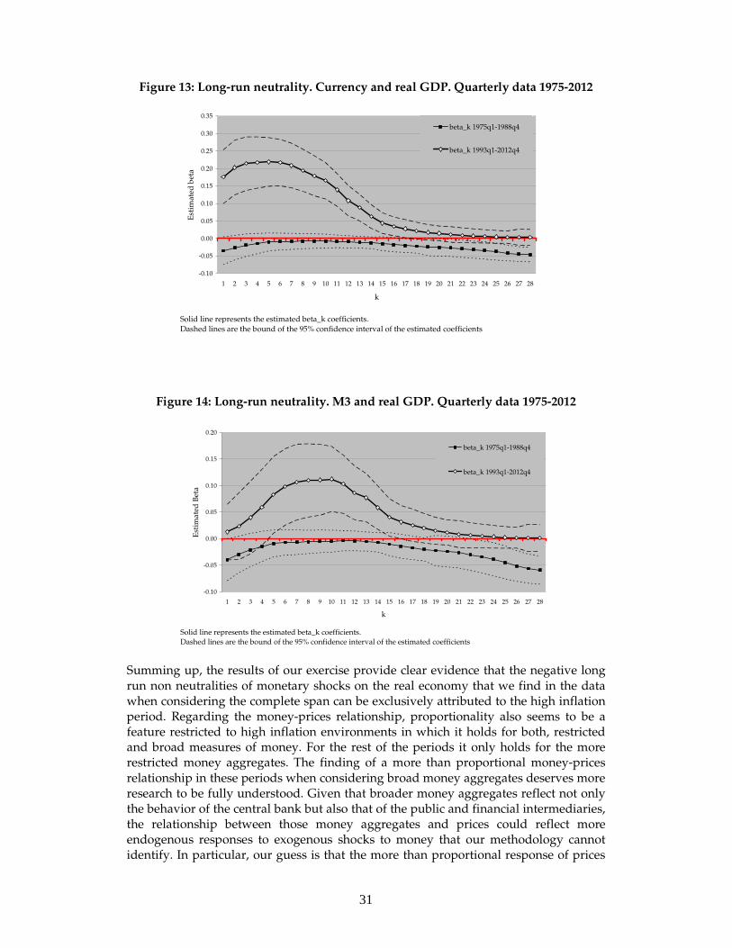
The results with respect to the long run money-real GDP relationship are quite interesting. The estimates for the high inflation period (1975q1-1988q4) clearly show that there are negative long run non-neutralities associated to permanent changes in money, considering both, currency and the M3 aggregate (see Figures 13 and 14). In case (iv), 1993q1-2012q4 period, the betas converge to 0, indicating that shocks to the aggregates –currency and M3- are neutral in the long run. Additionally, the pronounced U-inverted humped form depicted by the betas throughout the transition, suggest that the transitory effects of shocks to M3 on real activity are clearly positive. In fact, this is the only period in which the betas remain positive. Note that in this case we conduct the test using data at a higher frequency. This implies that our data incorporates some short–run variability not present at the annual frequency.

31

Figure 13: Long-run neutrality. Currency and real GDP. Quarterly data 1975-2012

Solid line represents the estimated beta_k coefficients. Dashed lines are the bound of the 95% confidence interval of the estimated coefficients

-0.10

-0.05

0.00

0.05

0.10

0.15

0.20

0.25

0.30

0.35

1 2 3 4 5 6 7 8 9 10 11 12 13 14 15 16 17 18 19 20 21 22 23 24 25 26 27 28 29 30

k

Est

imat

ed b

eta

beta_k 1975q1-1990q1 beta_k 1990q2-2012q4 beta_k 1994q1-2012q4

Neutrality

-0.10

-0.05

0.00

0.05

0.10

0.15

0.20

0.25

0.30

0.35

1 2 3 4 5 6 7 8 9 10 11 12 13 14 15 16 17 18 19 20 21 22 23 24 25 26 27 28

k

Est

imat

ed b

eta

beta_k 1975q1-1988q4

beta_k 1993q1-2012q4

Figure 14: Long-run neutrality. M3 and real GDP. Quarterly data 1975-2012

Solid line represents the estimated beta_k coefficients.

Dashed lines are the bound of the 95% confidence interval of the estimated coefficients

-0.10

-0.05

0.00

0.05

0.10

0.15

0.20

1 2 3 4 5 6 7 8 9 10 11 12 13 14 15 16 17 18 19 20 21 22 23 24 25 26 27 28

k

Est

ima

ted

Bet

a

beta_k 1975q1-1988q4

beta_k 1993q1-2012q4

Summing up, the results of our exercise provide clear evidence that the negative long run non neutralities of monetary shocks on the real economy that we find in the data when considering the complete span can be exclusively attributed to the high inflation period. Regarding the money-prices relationship, proportionality also seems to be a feature restricted to high inflation environments in which it holds for both, restricted and broad measures of money. For the rest of the periods it only holds for the more restricted money aggregates. The finding of a more than proportional money-prices relationship in these periods when considering broad money aggregates deserves more research to be fully understood. Given that broader money aggregates reflect not only the behavior of the central bank but also that of the public and financial intermediaries, the relationship between those money aggregates and prices could reflect more endogenous responses to exogenous shocks to money that our methodology cannot identify. In particular, our guess is that the more than proportional response of prices

32

to money could be associated to the high monetary instability to which economic agents were subject along the historical period we study -which at different amplitudes led to sharp positive as well as negative swings in broad measures of money. The increasing persistence of inflation over this period could probably contribute to this result too. Overall, these findings deserves more to be fully understand. VI. Conclusions Using the methodology developed by Fisher and Seater (1993) we test long run money neutrality for Argentina over the period 1900-2013. The long history of monetary instability and recurrent changes in the monetary framework that characterize the history of the country over these long span of time provides enough variability as to investigate the validity of these propositions. When considering the whole period we find significant non neutralities of exogenous permanent shocks on both prices and real GDP: Permanent exogenous shocks in money have a negative permanent effect on real output. At the same time this shocks reflect in more than proportional changes in prices. Since the economy went trough periods of low, moderate and high inflation as well as two hyperinflation episodes over this long span, we evaluate if the non neutralities that we find are in fact related to any of the periods rather than a feature of the whole sample. We identify structural breaks in the time series of different measures of money and prices. Based on these breaks, we split the sample and test neutrality for the identified sub periods. We corroborate that the negative non neutralities of exogenous permanent shocks to money on real GDP only remain for the high inflation period experienced by the country between 1975 and 1988. In all the other periods money is neutral with respect to real GDP. We also find that once we discard the hyperinflation episodes, the proportionality of prices with respect to money holds for all money aggregates in the high inflation period, a result in line with recent findings in the literature: Proportionality between money and prices seems to hold only in those periods in which the monetary authorities do not successfully respond to inflationary pressures. For the rest of the periods prices are proportional to money if restricted aggregates as the monetary base or currency are considered, but shocks to broader money aggregates lead to more than proportional changes in prices, a finding that deserves more research. Our findings corroborate that in high inflation environments there are permanent negative effects of innovations to money on the real economy, a concern of a large strand of the literature that focused on characterizing high inflation regimes and their real costs.

33

References Agiakoglou, C. and P. Newbold (1992): “Empirical Evidence on Dickey-Fuller type tests”, Journal of Time Series Analysis, 13, pp. 471-483 Bae, S. and R. Ratti (2000): “Long Run Neutrality, High Inflation, and Bank Insolvencies in Argentina and Brazil”, Journal of Monetary Economics, 46, pp. 581-604. Bai, J. y P. Perron (1998): “Estimating and Testing Linear Models with Multiple Structural Changes”, Econometrica, vol. 66(1), pp. 47-78, January. Bai, J. y P. Perron (2003): “Computation and Analysis of Multiple Structural Change Models”, Journal of Applied Econometrics, 18, 1, pp. 1-22. Baiocco, P. (1937): La economía bancaria argentina a través de sus índices más significativos en el período 1901-1935, Buenos Aires University, School of Economics. Ball, L. and G. Mankiw (1995): “Relative-Price Changes as Aggregate Supply Shocks”, The Quarterly Journal of Economics, vol. 110, N°1, pp.161-193. Barro, R. (1995): “Inflation and Economics Growth”, Bank of England, Quarterly Bulletin, (May), pp. 39-52. Barro, R. (1996): “Inflation and Growth”, Federal Reserve Bank of St. Louis Review, 78(3), pp. 153-169. Barro, R. and S. Fischer (1976): “Recent Developments in Monetary Theory”, Journal of Monetary Economics, 2, pp. 133-67. Basco, E., L. D ´Amato and L. Garegnani (2009): “Understanding the money - prices relationship under low and high inflation regimes: Argentina 1977 - 2006”, Journal of International Money and Finance. BCRA: Monetary and financial statistics, database in bank’s Web site (www.bcra.gov.ar). BCRA (various): Statistical Supplement of Revista Económica. BCRA (various): Statistical Bulletin. BCRA (various): Memories. BCRA (1990): “Información Estadística sobre Tasas de Interés”, Supplement of the Statistical Bulletin, June. Blejer, M. (1983): “On the Anatomy of Inflation: The Variability of Relative Commodity Prices in Argentina”, Journal of Money, Credit and Banking, vol. 15(4), pp. 469-82, November.

34

Boscher, J. and C. Ostrok (1994): “Long-Run Neutrality and Superneutrality in an ARIMA Framework: Comment”, The American Economic Review, Vol. 84, N° 5, pp. 1470-1473. Bozzoli G. and G. della Paolera (2014): “Evolución Monetaria, Regímenes de Banca Central y Teoría Cuantitativa del Dinero (QTM) en Argentina 1880-2010”, in Historia de las Instituciones Monetarias Argentinas R. Cortés Conde, L. D’Amato and J. Ortiz Batalla editors, Asociación Argentina de Economía Política, editorial Temas, forthcoming August 2014. Birentzwaig, A. E. (1982): Relevamiento estadístico de la economía argentina: 1900-1980, Banco de Análisis y Computación. Consultora de Investigaciones Económicas y Estadísticas (BAC), Buenos Aires. Bullard, J. (1999): “Testing Long-Run Monetary Neutrality Propositions: Lessons from the Recent Research”, Federal Reserve Bank of St. Louis Review, October/December. Bullard, J. and J. Keating (1995): “The long-run relationship between inflation and output in postwar economies”, Journal of Monetary Economics, vol. 36(3), pp. 477-496, December. Bunge, A. E. (1918): “Costo de la vida en la Argentina, de 1910 a 1917”, Revista de Economía Argentina, 1(1), pp. 39-63. Burdisso, T., E. Corso and S. Katz (2013): “Un efecto Tobin “perverso”: disrupciones monetarias y financieras y composición óptima del portafolio en Argentina”, Desarrollo Económico, Vol. 53, N° 209-210. Brock, P. L. (1989): “Reserve Requirements and the Inflation Tax”, Journal of Money, Credit and Banking, Vol. 21, N° 1 (February), pp. 106-121. Cagan, R. (1956): “The Monetary Dynamics of Hyperinflation”, in Studies in the Quantity Theory of Money, M. Friedman ed., Chicago: University of Chicago Press. Canavese, A. (1979): “La hipótesis estructural en la teoría de inflación”, Ensayos Económicos BCRA, N° 11, septiembre. Castagnino, T. and L. D’Amato (2013): “Régimen y dinámica inflacionaria subyacente: ¿comovimiento generalizado o ajuste de precios relativos?”, in Dinámica inflacionaria, persistencia y formación de precios y salarios, L. D´Amato, E. López Enciso and M. T. Ramírez G. (eds.), México: CEMLA. CEPAL (1958): “Anexo: algunos estudios especiales y estadísticas macroeconómicas preparados para el informe” in El desarrollo económico de la Argentina, Consejo Económico y Social, Santiago de Chile, June. Cortes Conde, R. (1979): El progreso argentino 1880-1914. Buenos Aires, Sudamericana, p. 226.

35

Cortes Conde, R. (1989): Dinero, deuda y crisis: Evolución fiscal y monetaria en la Argentina, 1862-1890, Buenos Aires: Sudamericana. Dabús, C. (2000): “Inflationary regimes and relative price variability: evidence from Argentina”, Journal of Development Economics, vol. 62(2), pp. 535-547, August. D´Amato L. and M. L. Garegnani (21013): “How Persistent is Inflation in Argentina?: Inflation Regimes and Price Dynamics in the Last 50 Years”, in Dinámica inflacionaria, persistencia y formación de precios y salarios, L . D’Amato, E. López Enciso and M. T. Ramírez G., editors, CEMLA. De Gregorio, J. and P. Guidotti (1995): “Financial development and economic growth”, World Development, vol. 23(3), pp. 433-448, March. De Grauwe, P. and M. Polan (2001): “Is Inflation Always and Everywhere a Monetary Phenomenon?”, CEPR Discussion Paper N° 2841. De Jong, D. N. (1992): “Integration vs. Trend Stationary in Time Series”, Econometrica, 60, pp. 423-433. Della Paolera, G. and J. Ortiz (1995): “Dinero, intermediación financiera y nivel de actividad en 110 años de historia económica argentina”, UTDT Working Papers, December. Della Paolera, G. and A. Taylor (2001): “Straining at the Anchor: The Argentine Currency Board and the Search for Macroeconomic Stability, 1880-1935”, NBER Series on Long Term Factors in Economic Growth, Chicago: Chicago University Press. Della Paolera, G. and A. Taylor (2003): A New Economic History of Argentina, Cambridge University Press. Díaz Alejandro, C. (1970): Essays on the Economic History of the Argentine Republic. New Haven: Yale University press. Díaz Alejandro, C. (1981): “Tipo de cambio y términos de intercambio en la República Argentina: 1913-76”, CEMA Research Series N° 22. Dirección General de Estadística de la Nación (1928): “Veinte años de estadística bancaria de la República Argentina 1908-1927”, coord.: R. Prebisch, Vol. 31. Dirección Nacional de Estadística y Censos (1945): Statistical Bulletin. Dirección Nacional de Estadística y Censos (1963): “Costo del Nivel de Vida en la Capital Federal”, Buenos Aires, February. Elliot, G., T. J. Rothenterberg and J. H. Stock (1996): “Efficient Tests for an Autoregresive Unit Root”, Econometrica, 64, pp. 813-836. Fanelli, J. M. and R. Frenkel (1995): “Estabilidad y estructura: interacciones en el crecimiento económico”, in Estabilización Macroeconómica, reforma estructural y comportamiento Industrial, Jorge Katz (ed.), Alianza Editorial, Buenos Aires.

36

Ferns, H. S. (1973): The Argentine Republic, 1516-1971. Newton Abbot: David and Charles. Ferreres, O. J. (2005): Dos siglos de economía argentina (1810-2004). Fundación Norte y Sur (Argentina), El Ateneo. Frenkel, R. (1979): “Decisiones de precio en alta inflación”, Desarrollo Económico, Vol. 19, N° 75, octubre-noviembre. Frenkel, R. (1989): “Inflación e hiperinflación, el infierno tan temido”, Revista Ciencia Hoy, Vol. 1, N° 3, abril-mayo 1989, pp. 52-61. Fischer, S. (1974): “Money and the Production Function”, Economic Inquiry, Vol. 12, Issue 4, pp. 517–533, December. Fischer, S. (1981): “Relative Shocks, Relative Price Variability, and Inflation”, Brookings Papers on Economic Activity, 2, pp. 381–431. Fisher, M. and J. Seater (1989): “Neutralities of Money”, Department of Economics and Business, unpublished manuscript, North Carolina University State University. Fisher, M. and J. Seater (1993): “Long-Run Neutrality and Superneutrality in ARIMA Framework”, American Economic Review, 83, June. Ford, A. (1962): The Gold Standard, 1880:1914: Britain and Argentina. Oxford: Clarendon Press. Gabrielli, F., G. McCandless and J. Rouillet (2004): “The Intertemporal Relation Between Money and Prices: Evidence from Argentina”, Latin American Journal of Economics, Vol. 41, 123, pp. 199-215. Gerchunoff, P. and L. Llach (2003): El ciclo de la ilusión y el desencanto: un siglo de políticas económicas argentinas, Ariel, Buenos Aires. Gerchunoff, P., F. Rocchi and G. Rossi (2008): Desorden y Progreso: Las Crisis Económicas Argentinas, 1870-1905, Edhasa. Geweke, J. F. (1986): “The Superneutrality of Money in the United States: An Interpretation of the Evidence”, Econometrica, vol. 54(1), pp. 1-21, January. Harberger, A. (1988): “World inflation revisited” in Economic effects of the government budget, edited by E. Helpman, A. Razin and E. Sadka, M.I.T Press: Cambridge and London, pp 217-237. Harberger, A. and S. Edwards (1980): “International Evidence on the Sources of Inflation”, Department of Economics, University of Chicago, mimeo, December.

Haug, A. and R. Lucas (1997): “Long-Run Neutrality and Superneutrality in an ARIMA Framework: Comment”, American Economic Review, vol. 87(4), pp. 756-59, September.

37

Hayek, F. A. (1931): Prices and Production, London: Routledge. Heymann, D. (1986): “Tres ensayos sobre inflación y políticas de estabilización”, Documentos de trabajo N° 18, Comisión Económica para América Latina y el Caribe (CEPAL), Naciones Unidas, Buenos Aires, febrero. Heymann, D. and A. Leijonhufvud (1995): High Inflation: The Arne Ryde Memorial Lectures, Oxford: Clarendon Press. Hicks, J. (1974): The Crisis of Keynesian Economics, New York: Basic Books. IEERAL (1986): “Estadísticas de la evolución económica de Argentina. 1913-1984”, Estudios N° 39, July/September. King, R. and M. Watson (1992): “Testing long run neutrality”, Working Paper Series, Macroeconomic Issues 92-18, Federal Reserve Bank of Chicago. King, R. and M. Watson (1994): “The post-war U.S. phillips curve: a revisionist econometric history”, Carnegie-Rochester Conference Series on Public Policy, Elsevier, vol. 41(1), pp. 157-219, December. King, R. and M. Watson (1997): “Testing long-run neutrality”, Economic Quarterly, Federal Reserve Bank of Richmond, issue Sum, pp. 69-101. Kormendi, R. C. and P. G. Meguire (1984): “Cross-Regime Evidence of Macroeconomic Rationality”, Journal of Political Economy, vol. 92(5), pp. 875-908, October. Kormendi, R. C. and P. G. Meguire (1985): “Macroeconomic Determinants of Growth: Cross-Country Evidence”, Journal of Monetary Economics, 16(2), pp. 141-163. Maddala, G. S. and I. M. Kim (2004): Unit Roots, Cointegration, and Structural Change. Themes in Modern Econometrics. Cambridge University Press. Mallon, R. and J. V. Sourrouille (1973): La política económica en una sociedad conflictiva, Amorrourtu, Buenos Aires. Martínez, R. G. (1999): “Recopilación de series históricas del producto y del ingreso”, CEPAL, Buenos Aires Office, April. McCallum, B. (1989): Monetary Economics, Theory and Policy, New York: Macmillan Publishing Company, London: Colier Macmillan Publishers. McCandless, G. T. and W. E. Weber (1995): “Some Monetary Facts”, Quarterly Review, Federal Reserve Bank of Minneapolis, Vol. 19, N° 3, (Summer), pp. 2-11. Mundell, R. (1963): "Inflation and Real Interest", Journal of Political Economy, vol. 71. Nelson, C. R. and C. I. Plosser (1982): “Trends and Random Walks in Macroeconomic Time Series”, Journal of Monetary Economics, 10, pp. 139-162.

38

Newey, W. and K. West (1987): “A Simple, Positive Semi-Definite, Heteroskedasticity and Autocorrelation Consistent Covariance Matrix”, Econometrica, Vol. 55, N°3, pp. 703-708, May. Ng, S. and P. Perron (2001): “Lag length selection and the construction of unit root tests with good size and power”, Econometrica, 69, pp. 1519–1554. Lucas, R. (1980); “Two Illustrations of the Quantity Theory of Money”, American Economic Review, 70(5), pp. 1005-1014 Olarra Jiménez, R. (1969): Evolución monetaria argentina, EUDEBA: Buenos Aires. Olivera, J. H. G. (1964): “On Structural Inflation and Latin-American Structuralism”, Oxford Economic Papers, November, Vol. XVI, pp. 321-32. Olivera, J. H. G. (1967): “Aspectos dinámicos de la inflación estructural”, Desarrollo Económico, Vol. 7, N° 27, Octubre-Diciembre, pp. 261-266. Orphanides, A. and R. M. Solow (1990): “Money, Inflation, and Growth”, in Handbook of Monetary Economics, B. M. Friedman and F. H. Hahn (eds.), Amsterdam: North Holland. Patinkin, D. (1956); Money, interest, and prices : an integration of monetary and value theory, Evanston, II : Row, Peterson and Company. Piñero, N. (1921): La moneda, el crédito y los bancos en la Argentina, Jesús Menéndez, Buenos Aires. Prebisch, R. (1922): “Anotaciones sobre nuestro medio circulante”, Revista de Ciencias Económicas, (mayo-junio) Rodrik, D. (1990): “How should structural adjustment programs be designed?”, World Development, vol. 18(7), pp. 933-947, July. Roubini, N. and X. Sala-i-Martin (1995): “A growth model of inflation, tax evasion, and financial repression”, Journal of Monetary Economics, vol. 35(2), pp. 275-301, April. Sargent T. and P. Surico (2011): “Two Illustrations of the Quantity Theory of Money: Breakdowns and Revivals”, American Economic Review, 101, February. Schwert, G. W. (1989): “Test for Unit Roots: a Monte Carlo Investigation”, Journal of Business and Economic Statistics, 7, pp. 147-159. Sheshinski, E. and Y. Weiss (1977): “Inflation and Costs of Price Adjustment”, Review of Economic Studies, vol. 44(2), pp. 287-303, June. Stock, J. H. (1994): “Unit Roots, Structural Breaks, and Trends” in R.F. Engle and D. L. McFadden (eds), Handbook of Econometrics, Vol. IV. Elsevier. Amsterdam. Stockman, A. C. (1981): “Anticipated inflation and the capital stock in a cash in-advance economy”, Journal of Monetary Economics, Vol. 8, Issue 3, pp. 387–393.

39

Tobin, J. (1965): “Money and Economic Growth”, Econometrica, Vol. 33, N° 4 (October), pp. 671-684. Tobin, J. (1969): “A General Equilibrium Approach to Monetary Theory”, Journal of Money, Credit and Banking, vol. 1(1), pp. 15-29, February. Tobin, J. (1992): “Money”, The New Palgrave Dictionary of Finance and Money, Vol. 2, pp. 770-779 and in The New Palgrave Dictionary of Economics, Second Edition, 2008. Tommasi, M. (1992): “Inflation and Relative Prices Evidence from Argentina”, UCLA Economics Working Papers 661, Department of Economics. Vázquez-Presedo, V. (1971-76): Estadísticas Históricas Argentinas, 2 vols., Buenos Aires. Ed Macchi. Vázquez-Presedo, V. (1988): Estadísticas Históricas Argentinas 1873-1973, Instituto de Economía Aplicada, Academia Nacional de Ciencias Económicas, Buenos Aires. Vázquez-Presedo, V. (1994): Estadísticas Históricas Argentinas 1970-1990, Instituto de Economía Aplicada, Academia Nacional de Ciencias Económicas, Buenos Aires. Walsh, C. E. (2003): Monetary Theory and Policy, third edition, Cambridge: MIT press. Wicksell, K. (1898): Geldzins und Güterpreise. Eine Untersuchung über die den Tauschwert des Geldes bestimmenden Ursachen, Jena: Gustav Fischer, (trad., 1936: Interest and Prices. A Study of the Causes Regulating the Value of Money, London: Macmillan). Williams, J. (1920): Argentine International Trade Under Inconvertible Paper Currency, 1880-1900. Cambridge, Mass: Harvard University Press.

40

Appendix: The specific methodology and sources of information of the series used in this paper are described below. Consumer prices The main source of information for this variable is the monthly time series of the Consumer Price Index (CPI) for the Gran Buenos Aires (April 2008 = 100) published by INDEC in its website. This series links up 1943, 1960, 1974, 1988 and 1999 series. Since January 2007 (inclusive) the previous series was completed with the monthly changes in the CPI computed by Buenos Aires City, and from January 2011 on, with the monthly change calculated by the National Congress (which is an average of several private estimations of CPI). Annual data was obtained by averaging the monthly indices of each year. Before 1943, the CPI series was completed using several sources. Between 1900 and 1913 two sources were consulted: from 1900 to 1910, inclusive, the average annual variations in the cost of a basic food basket presented in Cortes Conde (1979); and between 1911 and 1913, inclusive, the average annual changes in the cost of living index presented in Bunge (1918). These inflation rates match the variations of the CPI series found in Gerchunoff-Llach (2003). Finally, between 1914 and 1943 the average annual variations in the living cost of Buenos Aires city calculated by Dirección Nacional de Estadísticas y Censos (1963=100), published in Diaz Alejandro (1981), were used. Gross domestic product For the period 1900-1935 the data presented in the annex “Algunos estudios especiales y estadísticas macroeconómicas preparados para el informe” of ECLAC (1958) was used. This report exhibited annual series of GDP at 1950 prices for the period 1900-1955. Because or the absence of GDP deflators or nominal GDP series for this period, an implicit price index of GDP was constructed by the simple average of the annual change in consumer and wholesale prices of those years. Consumer prices correspond to the previously described series of CPI. As for wholesale prices, two sources were used: 1) for the period 1900-1913, annual variations in the wholesale price index (1884=100) of Della Paolera and Ortiz (1995); 2) for the period 1914-1935 annual variations in the wholesale price index (1960=100) from IEERAL (1986). For the period 1935-1992, inclusive, the GDP series at constant and current prices published in Martínez (ECLAC, 1999) were used. This publication compiles the national accounts series at 1950, 1960, 1970 and 1986 prices estimated by the Central Bank of Argentina. For the period 1993-2006, data of national accounts in 1993 prices published by the INDEC was considered. Because of the problems addressed in the official statistics since 2007, the series were completed with data of real and nominal GDP calculated by ARKLEMS. The final series of GDP at constant and current prices were calculated completing the national accounts at 1993 prices backwards with the real and nominal annual variations obtained from the sources mentioned before.

41

Deposit interest rate This is one of the variables that presented greater difficulties to set a consistent historical series. These difficulties are based on the diversity of deposit rates observed during the period, which reflects different concepts of return, risk and liquidity; changes in financial instruments; changes in the presentation of information; and different levels of regulation of the financial system. In this context, different sources were used to put together a series of interest rate on deposits in domestic currency for the period of interest. The series tries to reflect market interest rates, although regulated rates by the Central Bank were used in times when market rates were not available. No systematic records of interest rates for the period 1900-1924 were found. To fill this information gap, advertisements of banks in magazines of the time were used as a source of data (El Resumen, The Review of the River Plate and Handels-Zeitung). These ads showed interest rates offered by banks. However, the information is not homogeneous over time, and it is not uniform across banks, making the construction of a consistent series a difficult job. To deal with this problem only banks for which information was available more systematically in the period under analysis were considered: Banco de la Nación Argentina, Banco de Italia y del Río de la Plata, Banco Alemán Transatlántico, Banco Germánico de la América del Sud and Banco de la Provincia de Buenos Aires. These five institutions accounted for about half of system deposits. The interest rate of 3 months deposits in national currency was considered and simple averages of banks´ interest rates were calculated. In the absence of monthly data, the annual average was calculated with the data of December of each year and December of the previous year. For the period 1925-1931 no data on deposit interest rates in advertisements or other sources was found. Only data of discount rates of documents was available in Baiocco (1937). Then, data was completed assuming a linear decline in the spread, calculated as the difference between the discount rate of documents and the 90 days deposit rate for the years 1924 and 1932, and using the mentioned lending rate as reference for the years in between. Between 1932-1940 the monthly data of 3 months deposit rates taken from the Statistical Supplement of Revista Económica (BCRA’s economic journal) was used. When monthly data was not available (1932-1935), the annual average was calculated with the data of December of each year and December of the previous year. From 1940 on, the monthly data of 60 days or more days deposits rates reported by the Central Bank of Argentina on its website was used. However, the series has gaps in some years, which are related to the lack of market interest rates due to the regulations of the financial system. These gaps were filled with regulated interest rates. From April 1946 to June 1962 the series was completed with the regulated fixed-term deposits rates obtained from Central Bank’s Memories. Between July 1982 and May 1984 a new hole in statistics shows up because of the disappearance of market instruments, which was completed with fixed-term deposits rates set by the Central Bank (taken from the Supplement of the Statistical Bulletin of the Central Bank of June 1990). Finally,

42

between January and March 1990 there is a new gap, which was covered with non-regulated savings deposits rates taken from the previous source. Monetary aggregates The official data of monetary aggregates published by the Central Bank in the monetary and financial statistics section of its website begins in June 1940. This data includes: currency in circulation, monetary base, deposits of financial institutions on behalf of the Central Bank (needed to define the monetary base during periods of nationalization of deposits between 1946-1957 and 1973-1977), and bank deposits. In this last case, data is presented by type of deposit (current account deposits, savings deposits, fixed-time deposits, other deposits and acceptances), by currency (domestic and foreign currency, the latter appears discriminated from the mid 1980s), and by type of depositor (public and private sector). Backwards, monthly data was completed using various sources, which are described below. Figures from 1899 to 1900 were taken from Ferreres (2005), which is based on the statistical bulletin of Dirección Nacional de Estadística y Censos (DNEC, 1945) and Della Paolera and Taylor (2003). For the period 1901-1935 data from Baiocco (1937) was used. For currency in circulation held by the public and banks, Baiocco consulted Currency Boards´ monthly balances as a source of information. Since May 1935 (date in which the Central Bank was created) data was taken from the Statistical Supplement of Revista Económica, the economic journal published by the new monetary authority. This data excluded interbank deposits and included subsidiary currency, which corresponded to bills and coins of five pesos or less issued by the National Treasury and not backed by gold during the previous Currency Board regimen. In relation to banks´ liquidity, until the creation of the Central Bank a concept of minimum cash reserves (which included gold and paper money held by banks) was used; after that the minimum reserve requirements covered circulation held by banks and current account deposits of banks at the monetary authority. In the case of banks´ deposits, the information of Baiocco has as its source the Bureau of Economic Research of Banco de la Nación Argentina (the main public bank before the creation of the Central Bank in 1935). The data of deposits is not discriminated by currency denomination (gold or paper money pesos) neither by type of depositor (private or public sector). From 1926 on, interbank deposits are subtracted and deposits are classified in current account, savings, fixed-time and other deposits. To discriminate by type of deposit in previous years, information of deposits taken from Dirección General de Estadística (1928) was used. There, the data by type of deposit emerged from a survey of 27 banks between 1912 and 1926, and from a survey of 13 banks between 1908 and 1911. The shares of each type of deposits for those years were calculated, and for the period 1901-1908 the average share of 1908-1911 was utilized. Then these percentages were applied to total deposits series taken from Baiocco (1937). Finally, from July 1936 to December 1939 monthly data of the Statistical Supplement of Revista Económica, the economic journal of the Central Bank, was used. With the series described before, annual average of monthly data of currency in circulation (held by the public and by banks), monetary base (currency in circulation plus banks´ current account deposits at the Central Bank plus banks´ deposits on

43

behalf of Central Bank in times of deposits nationalization), M1 (currency in circulation outside the Central Bank plus current account deposits), M2 (M1 plus savings deposits), M3 (M2 plus fixed-time deposits, other deposits and acceptances) were computed, considering local and foreign currency deposits and private and public sector deposits. Annual averages were used in order to avoid distortions of relevant indicators, such as ratios to GDP or series in real terms, in periods of high inflation (because the series of GDP and CPI used as denominators are annual averages). Monthly data is available just from April 1907, when financial entities started to submit their balance sheet information to the Treasury on a monthly basis. Thus, for the period 1900-1906, the annual average was calculated as the average of December of each year and December of the previous year.